LA-UR-20-27569
October 2020

Heavy Handed Quest for Fixed Points in Multiple Coupling
Scalar Theories in the $\varepsilon$ Expansion

Hugh Osborn^a and Andreas Stergiou^b

^aDepartment of Applied Mathematics and Theoretical Physics, Wilberforce Road,

Cambridge CB3 0WA, England

^b Theoretical Division, MS B285, Los Alamos National Laboratory,

Los Alamos, NM 87545, USA

The tensorial equations for non trivial fully interacting fixed points at lowest order in the $\varepsilon$ expansion in $4-\varepsilon$ and $3-\varepsilon$ dimensions are analysed for $N$-component fields and corresponding multi-index couplings $\lambda$ which are symmetric tensors with four or six indices. Both analytic and numerical methods are used. For $N=5,6,7$ in the four-index case large numbers of irrational fixed points are found numerically where $||\lambda||^{2}$ is close to the bound found by Rychkov and Stergiou [1]. No solutions, other than those already known, are found which saturate the bound. These examples in general do not have unique quadratic invariants in the fields. For $N\geqslant 6$ the stability matrix in the full space of couplings always has negative eigenvalues. In the six index case the numerical search generates a very large number of solutions for $N=5$.

1 Introduction

There is a huge literature devoted to analysing fixed points using the $\varepsilon$ expansion for a very large number of physical systems and determining their critical exponents. A review covering many of the cases that have appeared in the literature is found in [2] and a wide range of known fixed points were also discussed by us with a different perspective in [3]. In many respects the $\varepsilon$ expansion is a universal solvent for understanding critical phenomena and builds on and extends the historic analysis based on Landau mean field theory. In practice it reduces to determining $\beta$-functions and anomalous dimensions in a loop expansion based on Feynman graphs. Results have been recently extended to seven loops in [4], as applied in [5], and with $O(N)$ symmetry to six [6] which have been extended to when the symmetry is reduced to $O(m)\times O(n)$ [7] and also cubic symmetry [8]. Using sophisticated resummation techniques to extend the $\varepsilon$ expansion to $\varepsilon=1$ there is remarkable agreement with results obtained by the bootstrap in three dimensions [9], although some tension also exists [10, 11].

The discovery of possible fixed points in any $\varepsilon$ expansion reduces to finding the zeros of the one loop $\beta$-functions in $4-\varepsilon$ dimensions. Higher loops provide perturbative corrections but do not generally eliminate the fixed point except at possible bifurcation points. Here the notionally small parameter $\varepsilon$ scales out and it is necessary to solve a tensorial quadratic equation for the symmetric couplings $\lambda_{ijkl}$ where the indices range from $1$ to $N$. The dimension of the space of symmetric 4-index couplings, $\tfrac{1}{24}N(N+1)(N+2)(N+3)$, increases rapidly with $N$ and the determination of possible fixed points consequently becomes non trivial for quite low $N$ without additional assumptions such as imposing a symmetry to reduce the number of independent couplings. Of course for $N=1$ the fixed point equations become totally trivial, giving rise to just the Ising fixed point. For $N=2,3$ historic discussions are contained in [12, 13] and a detailed analysis for $N=2$ is contained in [3]. More recently a careful analysis of the $N=3$ case is contained in [14] and this has also been extended to $N=4$ in [15].

There exist several examples of fixed points which appear for any $N$, most simply when there is $O(N)$ symmetry and just a single coupling, but there were until very recently no complete general results even when $N=3$. Various theorems for fixed points and their stability properties have been obtained in [16, 17, 18, 19]. More recently a fundamental bound was proved by Rychkov and Stergiou [1] which takes the form, after scaling out $\varepsilon$ and the usual factors of $16\pi^{2}$ which arise in a loop expansion,

$$S_{N}=||\lambda||^{2}=\lambda_{ijkl}\,\lambda_{ijkl}\leqslant\tfrac{1}{8}N\,,\quad N\geqslant 4\,.$$ (1.1)

For $N=2,3$ there are stronger bounds. When the bound is saturated there is a bifurcation point and the stability matrix develops a zero eigenvalue. Further bounds have been obtained by Hogervorst and Toldo [20, 21] including tighter results for $S_{N}$ when $N=2,3$. In terms of an $a$-function where the lowest order $\beta$-functions are expressed as a gradient [22, 3], $\beta_{ijkl}=\partial A/\partial_{\lambda_{ijkl}}=-\varepsilon\,\lambda_{ijkl}+{\rm O}(\lambda^{2})$, then at a fixed point

$$A_{*}=-\tfrac{1}{6}\,S_{N}\,\varepsilon^{3}\,.$$ (1.2)

Away from a fixed point with a renormalization group (RG) flow given by ${\dot{\lambda}}_{ijkl}=-\beta_{ijkl}$ then ${\dot{A}}=-||\beta||^{2}<0$. For given $N$ an RG flow from $\text{CFT}_{1}$ to $\text{CFT}_{2}$ cannot therefore exist unless $S_{N,\text{CFT}_{2}}>S_{N,\text{CFT}_{1}}$.

A related issue is the question of a lower bound for $S_{N}$. Of course for the Gaussian theory with $N$ free fields $S_{N}=0$. For two decoupled theories $S_{N}=S_{N_{1}}+S_{N_{2}}$ where $N=N_{1}+N_{2}$ and $S_{N_{1}},\,S_{N_{2}}$ correspond to fixed points with $N_{1},\,N_{2}$ fields. For $N$ decoupled Ising fixed points in our conventions $S_{N}=\frac{1}{9}N$ and assuming any perturbation of the $N$ decoupled Ising fixed point theory so as to generate a fully interacting theory decreases $A$ and hence increases $S_{N}$, then at any resulting fixed point

$$S_{N,{\rm fully\,interacting}}>\tfrac{1}{9}N\,.$$ (1.3)

However this is violated by $S_{N}$ for the fully interacting $O(N)$ symmetric fixed point if $N\geqslant 10$ (as $N\to\infty$ in this case $S_{N}\to 3$), which implies that for $N\geqslant 10$ there is no RG flow from the decoupled Ising to the $O(N)$ theory. Without imposing any condition that the fixed point not contain decoupled free theories [21] obtained $S_{N}>\frac{1}{9}$.

In previous literature the starting point has usually been the determination of all quartic polynomials in the scalar fields $\phi_{i}$ invariant under some subgroup $H$ of $O(N)$ for particular $N$. The choice of $H$ depends on the particular physical system for which critical exponents are to be found. For $N=4$ [23, 24] and $N=6$ [25, 26, 27] detailed investigations for all possible subgroups of $O(N)$, the corresponding spaces of quartic polynomials and associated fixed points was undertaken. Further analysis for low $N$ in $4-\varepsilon$ and $3-\varepsilon$ dimensions based on the symmetry groups for regular solids was described in [28]. In these discussions the condition that there is a unique quadratic polynomial, which may be taken as $\phi^{2}=\phi_{i}\phi_{i}$, is imposed. The fixed points found in this fashion are rational and generally have rational critical exponents. An emphasis in these papers is whether the fixed points in a particular symmetry class are stable or not. A fixed point is stable if there are no marginally relevant quartic operators, or equivalently the eigenvalues of the stability matrix, formed from the derivative of the $\beta$-function at the point where it vanishes, are all positive. Although not entirely evident in [23, 24] and [25, 26, 27] different symmetry groups may lead to the same fixed point.

Fixed points may apparently have different couplings corresponding to restrictions to different bases of quartic polynomials but if they are related by an $O(N)$ rotation or reflection they are equivalent. The fixed points which are determined by the zeros of the multi coupling $\beta$-functions may also correspond to decoupled theories, reducible to fixed point theories, including free theories, with lower $N$. Although the fixed points may be the same, the number of couplings and hence the dimension of the stability matrix may differ. This ensures that the question as to whether a fixed point is stable depends on the symmetry group which is initially imposed. A particular fixed point has identical values of $O(N)$ invariants such as $S_{N}$ in (1.1) although equality of $S_{N}$ by itself does not suffice to guarantee the same fixed point. This will be shown by particular examples later.

In this paper we follow an orthogonal approach by looking for solutions of the basic equations numerically for low $N$ where $S_{N}$ is close to the bound in (1.1). We focussed on such $S_{N}$ since we initially hoped to find fixed points where the bound was saturated. Although no such cases were found there are generically many fixed points wih increasing $N$ where $S_{N}$ is very close to $\tfrac{1}{8}N$. Our numerical search used the optimization algorithm Ipopt [29] through pygmo, which provides Python bindings of the C++ library pagmo [30]. Ipopt can perform constrained non linear optimization. The quantity $S_{N}$ was given as an objective to Ipopt, while the $\beta$-function equations were given as constraints. Ipopt was then called many times on a cluster, with a random initial point provided by pygmo. In many runs the algorithm failed to find a solution, but feasible solutions were frequently found too. Since our problem is non convex, different solutions were generally obtained in different runs. In our runs Ipopt entered the so-called “restoration phase” [29], in which the objective function $S_{N}$ was ignored and only the $\beta$-function equation violations were minimized. Thus, for a feasible solution, $S_{N}$ was not attempted to be maximised by Ipopt. Only the $\beta$-function equations were numerically satisfied, with a tolerance we chose to be $10^{-10}$. We subsequently improved the solutions obtained using SymPy’s nsolve or Mathematica’s FindRoot, in some cases to a tolerance of $10^{-200}$. We note here that it is not guaranteed that our method will find all possible solutions.

This method reproduces the known fixed points where $S_{N}$ is rational but also produces many irrational fixed points. Of course it is necessary to isolate those which are decoupled theories. For decoupled interacting fixed points the stability matrix has the eigenvalue 1 with degeneracy greater than one and for a free theory there are eigenvalues $-1$. Although our search is restricted to fixed points with $S_{N}$ close to the bound, we believe that it is possible to find all non trivial fixed points for $N=3,4$ and perhaps $N=5,6$. In the space of all quartic couplings the stability matrix has negative eigenvalues always when $N\geqslant 6$.

The irrational fixed points generally correspond to theories with two or more quadratic invariants. Such cases are not commonly considered but have recently been found to have relevance in discussions of conformal field theories (CFTs) at non zero temperature [31]. In many cases we are able to match the fixed points found numerically with results for fixed points in so called biconical theories, or various generalisations thereof. In the simplest case two theories which are separately $O(n),\,O(m)$ invariant are linked by a product of two singlet quadratic operators so the symmetry $O(n)\times O(m)$ is preserved. The fixed points arising from RG flow starting from the decoupled theory perturbed by the product of quadratic operators include one with the maximal $O(n+m)$ symmetry, but for $n\neq m$, and with suitable restrictions on $n,\,m$, they also lead to irrational fixed points with two quadratic invariants. The generalisations discussed here allow for several quadratic invariants. Such irrational fixed points were recognised long ago [32], for other literature see [33, 34, 35, 36].

In this paper in the next section we discuss the general features of the lowest order equations for the couplings $\lambda_{ijkl}$ and their decomposition under $O(N)$ and introduce $O(N)$ invariants $a_{0},a_{2},a_{4}$. Along with $S_{N}$ in (1.1) these serve to characterise different fixed points in an invariant fashion. Some bounds are obtained together with properties of stability matrix eigenvalues. In section 3 the fixed point equations are solved analytically for general $N$ assuming various symmetries, in particular the case when the symmetry is ${\cal S}_{N}$, the permutation group of $N$ objects. This includes previously known examples with cubic and tetrahedral symmetry. In section 4 fixed points which arise when two decoupled theories are perturbed by what can be regarded as double trace operators are described. These include so called biconical fixed points. They typically generate irrational fixed points although in some cases rational ones as well. Detailed results for all $N$ up to $N=7$ are presented in section 5. Where possible, numerical results are related to the analytic discussion earlier. Irrational fixed points for $N=4$ were found previously in [15]. This case is special in that fixed points which are degenerate at lowest order split at higher orders in $\varepsilon$. A similar discussion relating to the fixed point solutions for $\lambda_{ijklmn}$ is undertaken in section 6.

2 General $N$ Fixed Points

The basic algebraic equation determining fixed points at lowest order in the $\varepsilon$ expansion in $4-\varepsilon$ dimensions is

$$\lambda_{ijkl}=\lambda_{ijmn}\,\lambda_{klmn}+\lambda_{ikmn}\,\lambda_{jlmn}+\lambda_{ilmn}\,\lambda_{jkmn}\equiv S_{3,ijkl}\,\lambda_{ijmn}\,\lambda_{klmn}\,\,,$$ (2.1)

for $\lambda_{ijkl}$ the symmetric tensor determining the renormalisable couplings and we assume $i,j,k,l=1,\dots,N$. For any tensor $X_{ijkl}$, the action of the symmetriser $S_{n}$ is defined such $S_{n,ijkl}\,X_{ijkl}$ denotes the sum over the $n$ terms, with unit weight, which are the minimal necessary to ensure the sum is a fully symmetric four index tensor, if $X_{ijkl}$ is invariant under a subgroup $G_{X}\subseteq{\cal S}_{4}$ then $n=24/|G_{X}|$. With the potential

$$V(\phi)=\tfrac{1}{24}\,\lambda_{ijkl}\,\phi_{i}\phi_{j}\phi_{k}\phi_{l}\,,$$ (2.2)

(2.1) can be expressed more succinctly as

$$V(\phi)=\tfrac{1}{2}\,V_{ij}(\phi)V_{ij}(\phi)\,,\qquad V_{ij}(\phi)=\partial_{i}\partial_{j}V(\phi)\,.$$ (2.3)

The fixed point equation (2.1) is manifestly covariant under $O(N)$ and for any solution $\lambda_{ijkl}$ equivalent solutions are acting on $\lambda_{ijkl}$ with $O(N)$ rotations. Up to quadratic order there are $O(N)$ invariants in addition to $S_{N}$ in (1.1) given by

$$a_{0}=\lambda_{iijj}\,,\qquad a_{1}=\lambda_{ijkk}\,\lambda_{ijll}\,.$$ (2.4)

The symmetric coupling $\lambda_{ijkl}$ transforms as a four index tensor can be decomposed into the three possible $O(N)$ irreducible representations by writing

$$\lambda_{ijkl}={} d_{0}\,S_{3,ijkl}\,\delta_{ij}\,\delta_{kl}+S_{6,ijkl}\,\delta_{ij}\,d_{2,kl}+d_{4,ijkl}\,,$$ (2.5)

where $d_{2,ij}$ and $d_{4,ijkl}$ are symmetric and traceless rank two and rank four tensors; $d_{2,ij}$ is determined by

$$(N+4)\,d_{2,ij}=\lambda_{ijkk}-(N+2)\,d_{0}\,\delta_{ij}\,,$$ (2.6)

and then $d_{4,ijkl}$ is given in terms of $\lambda_{ijkl}$ by subtraction of the $d_{0},\,d_{2}$ pieces. Following Hogervorst and Toldo [20, 21]

$$a_{0}={} N(N+2)d_{0}\,,\qquad a_{2}=(N+4)^{2}||d_{2}||^{2}=a_{1}-\tfrac{1}{N}\,a_{0}{\!}^{2}\,,$$

$$a_{4}={} ||d_{4}||^{2}=S_{N}-\tfrac{6}{N+4}\,a_{2}-\tfrac{3}{N(N+2)}\,a_{0}{\!}^{2}\,.$$ (2.7)

If $\alpha_{r}$ are the eigenvalues of $\lambda_{ijkk}$ then $a_{2}=\sum_{r<s}(\alpha_{r}-\alpha_{s})^{2}/N$ and crucially it follows that

$$a_{2}=0\quad\Leftrightarrow\quad\lambda_{ijkk}=\alpha\,\delta_{ij}\,,\quad\alpha=\tfrac{1}{N}\,a_{0}\,.$$ (2.8)

For decoupled theories $\lambda_{1\cup 2,ijkl}=\lambda_{1,ijkl}+\lambda_{2,ijkl}$ where $\lambda_{1}\cdot\lambda_{2}=0$. In this case $a_{0},\,a_{1},\,S_{N}$ are additive though $a_{2},\,a_{4}$ are not,

$$a_{2,1\cup 2}=a_{2,1}+a_{2,2}+\frac{1}{N_{1}N_{2}\,N}\big{(}N_{2}\,a_{0,1}-N_{1}\,a_{0,2}\big{)}^{2}\,,\quad N=N_{1}+N_{2}\,.$$ (2.9)

Other $O(N)$ invariants are given by the $N$ eigenvalues $\{\gamma\}$ of $[\Gamma_{ij}]$ where

$$\Gamma_{ij}=\lambda_{iklm}\,\lambda_{jklm}\,,\qquad\Gamma_{ij}v_{j}=\gamma\,v_{i}\,,\quad{\textstyle\sum}\gamma=S_{N}\,.$$ (2.10)

These determine the lowest order anomalous dimensions for the $N$-component fields $\phi_{i}$ at the fixed point which are $\tfrac{1}{12}\gamma\,\varepsilon$. If (2.8) is satisfied then from (2.1)

$$2\,\Gamma_{ij}=(\alpha-\alpha^{2})\,\delta_{ij}\,.$$ (2.11)

Conversely for $a_{2}$ non zero $\Gamma_{ij}$ should not be proportional to $\delta_{ij}$ and there are necessarily different eigenvalues $\gamma$. For all eigenvalues $\gamma$ equal then since $[\Gamma_{ij}]$ is a positive matrix it is necessary that $0\leqslant\gamma\leqslant\tfrac{1}{8}$; saturating the upper bound is equivalent to (1.1).

Further invariants are also given by the $\frac{1}{24}N(N+1)(N+2)(N+3)$ eigenvalues $\{\kappa\}$ of the stability matrix at the fixed point which are determined by

$$(\kappa+1)\,v_{ijkl}=S_{6,ijkl}\,\lambda_{ijmn}\,v_{klmn}={} \lambda_{ijmn}\,v_{klmn}+\lambda_{ikmn}\,v_{jlmn}+\lambda_{ilmn}\,v_{jkmn}$$

$${}+\lambda_{klmn}\,v_{ijmn}+\lambda_{jlmn}\,v_{ikmn}+\lambda_{jkmn}\,v_{ilmn}\,,$$ (2.12)

for $v_{ijkl}$ symmetric. In this case

$${\textstyle\sum}\,\kappa=\tfrac{1}{2}(N+2)(N+3)a_{0}-\tfrac{1}{24}N(N+1)(N+2)(N+3)\,.$$ (2.13)

Furthermore

$${\textstyle\sum}\,(\kappa+1)^{2}=\tfrac{1}{2}(N+4)(N+5)S_{N}+4(N+4)a_{1}+a_{0}{\!}^{2}\,.$$ (2.14)

A solution is always obtained by taking $v_{ijkl}\to\lambda_{ijkl}$ giving, by virtue of (2.1), $\kappa=1$. This is in general non degenerate except for decoupled theories. Directly from (2.12) and (2.1)

$$(1-\kappa)\lambda_{ijkl}v_{ijkl}=0\,.$$ (2.15)

Any non zero

$$v_{ijkl}=\omega_{ir}\,\lambda_{rjkl}+\omega_{jr}\,\lambda_{irkl}+\omega_{kr}\,\lambda_{ijrl}+\omega_{kr}\,\lambda_{ijkr}\,,\quad\omega_{ij}=-\omega_{ji}\,,$$ (2.16)

gives solutions of (2.12) with $\kappa=0$. In general $\omega_{ij}$ corresponds to elements of the Lie algebra of $O(N)$. The number of zero modes (2.16) is given by $\tfrac{1}{2}N(N-1)-\dim\mathfrak{H}$ where $\mathfrak{H}$ is the Lie algebra of the unbroken subgroup $H\subset O(N)$ which leaves $\lambda_{ijkl}$ invariant.

The eigenvalue equations may be extended to $\phi^{2}$ and $\phi^{3}$ operators where the anomalous dimensions are determined by

$$\ \mu\,v_{ij}=\lambda_{ijkl}\,v_{kl}\,,\qquad\nu\,v_{ijk}=\lambda_{ijlm}\,v_{klm}+\lambda_{jklm}\,v_{ilm}+\lambda_{kilm}\,v_{jlm}\,,$$ (2.17)

where

$${\textstyle\sum}\,\mu=a_{0}\,,\qquad{\textstyle\sum}\,\nu=(N+2)a_{0}\,.$$ (2.18)

A solution of the eigenvalue equation for $\nu$ is obtained with $\nu=1$ by taking $v_{ijk}\to\lambda_{ijkl}v_{l}$, for any vector $v_{l}$, so this is $N$-fold degenerate.

For decoupled theories 1 and 2

$$\{\kappa\}_{1\cup 2}={} \{\kappa\}_{1}\cup\{\kappa\}_{2}\cup\big{(}\{\nu\}_{1}{\mathds{1}}_{N_{2}}-1\big{)}\cup\big{(}{\mathds{1}}_{N_{1}}\{\nu\}_{2}-1\big{)}$$

$${}\cup\big{(}\{\mu\}_{1}{\mathds{1}}_{\frac{1}{2}N_{2}(N_{2}+1)}+{\mathds{1}}_{\frac{1}{2}N_{1}(N_{1}+1)}\{\mu\}_{2}-1\big{)}\,,$$ (2.19)

where we have used the result that the anomalous dimension of $\phi$ is zero at lowest order. This satisfies, by using (2.13) and (2.14),

$${\textstyle\sum_{1\cup 2}}\,\kappa={} \big{(}\tfrac{1}{2}(N_{1}+2)(N_{1}+3)+(N_{1}+1)N_{2}+\tfrac{1}{2}N_{2}(N_{2}+1)\big{)}a_{0,1}+1\leftrightarrow 2$$

$${}-\big{(}\tfrac{1}{24}N_{1}(N_{1}+1)(N_{1}+2)(N_{1}+3)+\tfrac{1}{6}N_{1}(N_{1}+1)(N_{1}+2)N_{2}+1\leftrightarrow 2\big{)}$$

$${}-\tfrac{1}{4}N_{1}(N_{1}+1)N_{2}(N_{2}+1)\,,$$ (2.20)

which satisfies (2.13) with $N=N_{1}+N_{2}$ since $a_{0}=a_{0,1}+a_{0,2}$. For the $n$-fold free theory $\kappa=-1(\frac{1}{24}n(n+1)(n+2)(n+3)),\ \nu=0(\frac{1}{6}n(n+1)(n+2)),\ \mu=0(\frac{1}{2}n(n+1))$. As a consequence of the results for eigenvalues with $\nu=1$ there will be $2N_{1}N_{2}$ zero eigenvalues for $\{\kappa\}_{1\cup 2}$, in addition to those arising from $\{\kappa\}_{1}$ or $\{\kappa\}_{2}$, for two decoupled interacting theories. For a decoupled fixed point formed by $n$-fold free fields and a $N$-component interacting fixed point $FP_{N}$ there are $Nn$ extra zero modes besides those present in $FP_{N}$. For $n$ decoupled interacting theories $\{\kappa\}_{1\cup 2\cup\dots\cup n}$ contains $2\sum_{1\leqslant i<j\leqslant n}N_{i}N_{j}$ extra zero modes.

2.1 Decomposition of Fixed Point Equation

Applying (2.5) in (2.1) gives rise to three separate equations

$$\hskip-28.45274ptd_{0}={} (N+8)\,d_{0}{}^{2}+\tfrac{(N+4)(N+16)}{N(N+2)}\,||d_{2}||^{2}+\tfrac{2}{N(N+2)}\,||d_{4}||^{2}\,,$$ (2.21a)

$$d_{2,ij}={} (N+16)\,d_{0}\,d_{2,ij}+\tfrac{2}{N+4}(5N+32)\,\big{(}d_{2,ik}\,d_{2,jk}-\tfrac{1}{N}\,\delta_{ij}\,||d_{2}||^{2}\big{)}$$

$${}+\tfrac{1}{N+4}(N+16)\,d_{4,ijkl}\,d_{2,kl}+\tfrac{2}{N+4}\,\big{(}d_{4,iklm}\,d_{4,jklm}-\tfrac{1}{N}\,\delta_{ij}\,||d_{4}||^{2}\big{)}\,,$$ (2.21b)

$$d_{4,ijkl}={} 12\,d_{0}\,d_{4,ijkl}$$

$${}+(N+16)\,S_{3,ijkl}\big{(}d_{2,ij}\,d_{2,kl}-\tfrac{2}{N+4}(\delta_{ij}\,d_{2,km}\,d_{2,lm}+\delta_{kl}\,d_{2,im}\,d_{2,jm})$$

$$\hskip 193.47882pt{}+\tfrac{2}{(N+2)(N+4)}\,\delta_{ij}\,\delta_{kl}\,||d_{2}||^{2}\big{)}$$

$${}+S_{3,ijkl}\big{(}d_{4,ijmn}\,d_{4,klmn}-\tfrac{2}{N+4}(\delta_{ij}\,d_{4,kmnp}\,d_{4,lmnp}+\delta_{kl}\,d_{4,imnp}\,d_{4,jmnp})$$

$$\hskip 213.39566pt{}+\tfrac{2}{(N+2)(N+4)}\,\delta_{ij}\,\delta_{kl}\,||d_{4}||^{2}\big{)}$$

$${}+6\big{(}S_{4,ijkl}\,d_{4,ijkm}\,d_{2,lm}-\tfrac{2}{N+4}\,S_{6,ijkl}\,d_{4,ijmn}\,d_{2,mn}\,\delta_{kl}\big{)}\,.$$ (2.21c)

From (2.1) or (2.21a)

$$a_{0}=a_{1}+2\,S_{N}\,,\qquad a_{0}\big{(}1-\tfrac{N+8}{N(N+2)\,}a_{0}\big{)}=2\,a_{4}+\tfrac{N+16}{N+4}\,a_{2}\,.$$ (2.22)

Hence using (2.7), (2.22) we obtain the bounds

$$a_{0}<\tfrac{N(N+2)}{N+8}\,,\quad S_{N}+\tfrac{1}{2}\,a_{2}=\tfrac{1}{8}N-\tfrac{1}{2N}\big{(}a_{0}-\tfrac{1}{2}N\big{)}^{2}\leqslant\begin{cases}\tfrac{1}{8}N\,,\ \ &N\geqslant 4\\ \tfrac{3N(N+2)}{(N+8)^{2}}\,,&N<4\end{cases}\,.$$ (2.23)

This is just the Rychkov–Stergiou bound [1] as extended by Hogervorst–Toldo [20, 21]; the Rychkov–Stergiou case arises for $N\geqslant 4$ when $a_{2}=0$. This bound is saturated for $a_{0}=\tfrac{1}{2}N$, which is necessary for the sum of two decoupled theories saturating the bound to also satisfy the bound since (2.9) requires $N_{2}\,a_{0,1}-N_{1}\,a_{0,2}=0$. The bound on $a_{0}$ is saturated for the $O(N)$ symmetric theory. With this bound on $a_{0}$ then (2.13) requires $\sum\kappa<0$ when $N\geqslant 6$. If (1.1) is saturated then necessarily $a_{2}=0$ and from (2.8) and (2.11) then $\Gamma_{ij}=\tfrac{1}{8}\,\delta_{ij}$.

The fixed point equations can be reduced for any basis of 4 and 2 index symmetric traceless tensors $\{d_{r,ijkl},\,{\hat{d}}_{a,ij}\}$, $r=1,\dots,p,\ a=1,\dots,q$, satisfying

$$\tfrac{1}{2}S_{6,ijkl}\,d_{r,ijmn}\,d_{s,klmn}=a_{rs}\,S_{3,ijkl}\,\delta_{ij}\delta_{kl}+{\textstyle\sum_{t}}\,b_{rs}{}^{t}d_{t,ijkl}+{\textstyle\sum_{b}}\,c_{rs}{}^{a}\,S_{6,ijkl}\,\delta_{ij}{\hat{d}}_{a,kl}\,,$$ (2.24a)

$$S_{4,ijkl}\,d_{r,ijkm}\,{\hat{d}}_{a,lm}={\textstyle\sum_{b}}\,e_{ra}{}^{b}\,S_{6,ijkl}\,\delta_{ij}{\hat{d}}_{b,kl}+{\textstyle\sum_{s}}\,f_{ra}{}^{s}\,d_{s,ijkl}\,,$$ (2.24b)

$$\tfrac{1}{2}S_{6,ijkl}\,{\hat{d}}_{a,ij}\,{\hat{d}}_{b,kl}=\tfrac{2}{N+4}\,{\hat{a}}_{ab}\,S_{3,ijkl}\,\delta_{ij}\delta_{kl}+{\textstyle\sum_{r}}\,{\hat{b}}_{ab}{}^{r}d_{r,ijkl}+{\textstyle\sum_{c}}\,{\hat{c}}_{ab}{}^{c}\,S_{6,ijkl}\,\delta_{ij}{\hat{d}}_{c,kl}\,,$$ (2.24c)

where it is necessary that $a_{rs},\,b_{rs}{}^{t},\,c_{rs}{}^{a}$ are symmetric under $r\leftrightarrow s$ and similarly ${\hat{a}}_{ab},\,{\hat{b}}_{ab}{}^{r},\,{\hat{c}}_{ab}{}^{c}$ for $a\leftrightarrow b$. Consistency between (2.24a), (2.24b) and (2.24c) requires

$${\textstyle\sum_{u}}\,b_{rs}{}^{u}a_{ut}=b_{rst}=b_{(rst)}\,,\quad{\textstyle\sum_{d}}\,{\hat{c}}_{ab}{}^{d}{\hat{a}}_{dc}={\hat{c}}_{abc}={\hat{c}}_{(abc)}\,,$$

$${\hat{b}}_{ab\hskip 0.5ptr}={\textstyle\sum_{s}}\,{\hat{b}}_{ab}{}^{s}{}a_{sr}=3\,e_{ra}{}^{c}{\hat{a}}_{cb}=3\,e_{r\hskip 0.5ptab}\,,\quad 4\,c_{rs\hskip 0.5pta}=4\,{\textstyle\sum_{b}}\,c_{rs}{}^{b}\,{\hat{a}}_{ba}=f_{ra}{}^{t}a_{ts}=f_{ra\hskip 0.5pts}\,.$$ (2.25)

From (2.24c)

$$({\hat{d}}_{a}\vee_{2}{\hat{d}}_{b})=\tfrac{1}{2}S_{2,ij}\,{\hat{d}}_{a,ik}\,{\hat{d}}_{b,jk}=\tfrac{N+2}{N+4}\,{\hat{a}}_{ab}\,\delta_{ij}+\tfrac{1}{2}(N+4)\,{\textstyle\sum_{c}}\,{\hat{c}}_{ab}{}^{c}\,{\hat{d}}_{c,ij}\,,$$ (2.26)

The non associative algebra of symmetric matrices defined the symmetric product $\vee_{2}$ is a Jordan algebra since, for $U,V$ symmetric, $U\vee_{2}(V\vee_{2}(U\vee_{2}U))=(U\vee_{2}V)\vee_{2}(U\vee_{2}U)$. If (2.26) is reducible to the form

$${\hat{d}}_{a,ik}\,{\hat{d}}_{b,jk}=\delta_{ab}\big{(}\delta_{ij}+{\hat{c}}_{a}\,{\hat{d}}_{a,ij}\big{)}\,.$$ (2.27)

then all solutions are expressible in terms of projection operators with

$${\hat{c}}_{a}=\frac{n_{a}-m_{a}}{\sqrt{n_{a}\,m_{a}}}\,,\qquad n_{a}+m_{a}=N\,.$$ (2.28)

If (2.24c) is regarded as defining ${\textstyle\sum_{r}}\,{\hat{b}}_{ab}{}^{r}d_{r,ijkl}$ then inserting in (2.24b) and using (2.26) gives

$${\textstyle\sum_{s}}\,{\hat{b}}_{ab}{}^{s}\,f_{sc}{}^{r}={} {\textstyle\sum_{d}}\big{(}2(N+4)\,{\hat{c}}_{c(a}{}^{d}\,{\hat{b}}_{b)d}{}^{r}-4\,{\hat{c}}_{ab}{}^{d}\,{\hat{b}}_{dc}{}^{r}\big{)}\,,$$

$${\textstyle\sum_{r}}\,{\hat{b}}_{ab}{}^{r}\,{e}_{r\hskip 0.1ptc}{}^{d}={} \tfrac{1}{N+4}\big{(}2(N+2)\,\delta_{(a}{}^{d}\,{\hat{a}}_{b)c}\,-4\,\delta_{c}{}^{d}\,{\hat{a}}_{ab}\big{)}$$

$${}+{\textstyle\sum_{e}}\big{(}2(N+4)\,{\hat{c}}_{c(a}{}^{e}\,{\hat{c}}_{b)e}{}^{d}-(N+8)\,{\hat{c}}_{ab}{}^{e}\,{\hat{c}}_{ec}{}^{d}\big{)}\,.$$ (2.29)

Using (2.25)

$${\textstyle\sum_{r,s}}\,{\hat{b}}_{ab}{}^{r}\,{\hat{b}}_{cd}{}^{s}\,a_{rs}{}={} 3\,\tfrac{N+2}{N+4}({\hat{a}}_{ac}\,{\hat{a}}_{bd}+{\hat{a}}_{ad}\,{\hat{a}}_{bc})-\tfrac{12}{N+4}\,{\hat{a}}_{ab}\,{\hat{a}}_{cd}$$

$${}+3(N+4)\big{(}{\hat{c}}_{ac}{}^{e}\,{\hat{c}}_{ebd}+{\hat{c}}_{bc}{}^{e}\,{\hat{c}}_{ead}\big{)}-3(N+8)\,{\hat{c}}_{ab}{}^{e}\,{\hat{c}}_{ecd}\,.$$ (2.30)

Writing

$$d_{0}=\lambda\,,\qquad d_{2,ij}={\textstyle\sum_{a}}\,h^{a}\,{\hat{d}}_{a,ij}\,,\qquad d_{4,ijkl}={\textstyle\sum_{r}}\,g^{r}\,d_{r,ijkl}\,,$$ (2.31)

so that

$$||d_{2}||^{2}=\tfrac{1}{N+4}N(N+2)\,{\textstyle\sum_{ab}}\,{\hat{a}}_{ab}h^{a}h^{b}\,,\qquad||d_{4}||^{2}=\tfrac{1}{2}N(N+2)\,{\textstyle\sum_{rs}}\,a_{rs}g^{r}g^{s}\,,$$ (2.32)

the lowest order fixed point equations for the $p+q+1$ couplings $\lambda,\,g^{r},\,h^{a}$ from (2.21a), (2.21b), (2.21c) are then

$$\lambda={} (N+8)\lambda^{2}+{\textstyle\sum_{r,s}}\,a_{rs}\,g^{r}g^{s}+(N+16)\,{\textstyle\sum_{a,b}}\,{\hat{a}}_{ab}\,h^{a}h^{b}\,,$$

$$g^{r}={} 12\,\lambda\,g^{r}+{\textstyle\sum_{s,t}}\,b_{st}{}^{r}g^{s}g^{t}+(N+16)\,{\textstyle\sum_{a,b}}\,{\hat{b}}_{ab}{}^{r}h^{a}h^{b}+6\,{\textstyle\sum_{s,a}}\,f_{sa}{}^{r}\,g^{s}h^{a}\,,$$

$$h^{a}={} (N+16)\big{(}\lambda\,h^{a}+\tfrac{1}{2}\,{\textstyle\sum_{r,b}}\,e_{rb}{}^{a}\,h^{b}g^{r}\big{)}+(5N+32)\,{\textstyle\sum_{b,c}}\,{\hat{c}}_{bc}{}^{a}h^{b}h^{c}+{\textstyle\sum_{r,s}}\,c_{rs}{}^{a}g^{r}g^{s}\,,$$ (2.33)

where $f_{sa}{}^{r},\,e_{rb}{}^{a}$ can be eliminated using (2.25).

2.2 Further Bounds

A general analysis of (2.21a), (2.21b), (2.21c) is not straightforward. In general $d_{0}\leqslant\frac{1}{N+8}$, which is equivalent to the $a_{0}$ bounds in (2.23). If (1.1) is to be saturated, then $d_{2,ij}=0$ and the equations simplify to

$$d_{0}=(N+8)\,d_{0}{}^{2}+\tfrac{2}{N(N+2)}\,||d_{4}||^{2}\,,\quad d_{4,iklm}\,d_{4,jklm}=\tfrac{1}{N}\,\delta_{ij}\,||d_{4}||^{2}\,,$$

$$(1-12\,d_{0})\,d_{4,ijkl}=S_{3,ijkl}\big{(}d_{4,ijmn}\,d_{4,klmn}-\tfrac{2}{N(N+2)}\,\delta_{ij}\,\delta_{kl}\,||d_{4}||^{2}\big{)}\,.$$ (2.34)

The last two equations are equivalent to writing

$$d_{4,ijmn}\,d_{4,klmn}=\tfrac{1}{N-1}\,a\big{(}\tfrac{1}{2}N(\delta_{ik}\delta_{jl}+\delta_{il}\delta_{jk})-\delta_{ij}\delta_{kl}\big{)}+\tfrac{1}{3}\,b\,d_{4,ijkl}+w_{ijkl}\,,$$ (2.35)

where

$$w_{ijkl}={} \tfrac{1}{3}\big{(}2\,d_{4,ijmn}\,d_{4,klmn}-d_{4,ikmn}\,d_{4,jlmn}-d_{4,ilmn}\,d_{4,jkmn}\big{)}$$

$${}+\tfrac{1}{3N(N-1)}\,||d_{4}||^{2}\big{(}2\,\delta_{ij}\delta_{kl}-\delta_{ik}\delta_{jl}-\delta_{il}\delta_{jk}\big{)}\,,$$

$$a=\tfrac{2}{N(N+2)}\,||d_{4}||^{2}\,,\qquad b=1-12\,d_{0}\,.$$ (2.36)

$w_{ijkl}$ is a mixed symmetry tensor satisfying $w_{ijkl}=w_{(ij)kl}=w_{klij}$, $w_{i(jkl)}=0$ and $w_{ijkk}=0$. With this definition for $w_{ijkl}$

$$||w||^{2}=w_{ijkl}w_{ijkl}=\tfrac{2}{3}\,d_{4,ijmn}d_{4,klmn}\big{(}d_{4,ijpq}d_{4,klpq}-d_{4,ikpq}d_{4,jlpq}\big{)}-\tfrac{2}{3N(N-1)}\,||d_{4}||^{4}\,.$$ (2.37)

Substituting (2.35) ensures this is just an identity.

Higher rank tensors can be formed from $d_{4,ijkl}$. There is a symmetric 6-index tensor

$$S_{6,ijklmn}=d_{(ijk|p}\,d_{lmn)p}-\frac{3\,b}{N+8}\,\delta_{(ij}\,d_{klmn)}-\frac{3\,a}{N+4}\,\delta_{(ij}\,\delta_{kl}\,\delta_{mn)}\,,$$ (2.38)

and a corresponding mixed symmetry symmetry tensor

$$M_{6,ijklmn}={} d_{ij(k|p}\,d_{lmn)p}-d_{i(kl|p}\,d_{mn)jp}$$

$${}+\frac{b}{3(N-2)}\big{(}\delta_{ij}\,d_{klmn}-\delta_{i(k}\,d_{lmn)j}-\delta_{j(k}\,d_{lmn)i}+\delta_{(kl}\,d_{mn)ij}\big{)}$$

$${}+\frac{a}{N-1}\big{(}\delta_{ij}\,\delta_{(kl}\,\delta_{mn)}-\delta_{i(k}\,\delta_{lm}\,\delta_{n)j}\big{)}-\frac{5}{N+4}\,w_{ij(kl}\,\delta_{mn)}\,.$$ (2.39)

Then

$$||S_{6}||^{2}=\frac{1}{40}\,N(N+2)^{2}\bigg{(}\frac{(N-2)(N+14)}{(N-1)(N+4)}\,a^{2}+\frac{2}{N+8}\,a\,b^{2}\bigg{)}-\frac{9}{20}\,||w||^{2}\,,$$ (2.40)

and

$$||M_{6}||^{2}=\frac{5}{48}\,N(N+2)^{2}\bigg{(}\frac{N-2}{N-1}\,a^{2}-\frac{2}{9(N-2)}\,a\,b^{2}\bigg{)}+\frac{5(N-16)}{24(N+4)}\,||w||^{2}\,.$$ (2.41)

In general (2.41) gives an upper bound on $b$ and hence bounds on $d_{0}$, clearly

$$b^{2}\leqslant\tfrac{9(N-2)^{2}}{2(N-1)}\,a\,,\quad N\leqslant 16\,.$$ (2.42)

For $N=3$ $w$ and $M_{6}$ must vanish and hence we require $a=\tfrac{4}{9}\,b^{2}$ assuming $d_{2}=0$ and $d_{4}\neq 0$. This gives $||d_{4}||^{2}=\frac{10}{3}(1-12\,d_{0})^{2}$, and hence $d_{0}=\frac{1}{15},\,||d_{4}||^{2}=\tfrac{2}{15}$ implying $a_{0}=1,\,S=\frac{1}{3}$ or $d_{0}=\frac{4}{45},\,||d_{4}||^{2}=\tfrac{2}{135}$ with $a_{0}=\tfrac{4}{3},\,S=\frac{10}{27}$. From (2.36)

$$\bigg{(}1-\frac{12}{N(N+2)}\,a_{0}\bigg{)}^{\!2}\leqslant\frac{9(N-2)^{2}}{N(N-1)(N+2)}\,a_{4}\,,\quad a_{2}=0\,,\ a_{4}>0\,,\ \ N\leqslant 16\,.$$ (2.43)

Combining with (2.23) this gives

$$\tfrac{1}{3}\,N\leqslant a_{0}\leqslant\tfrac{2}{3}(N-1)\,,\qquad a_{2}=0\,,\ a_{4}>0\,,\ N\leqslant 16\,.$$ (2.44)

When this bound is saturated it is necessary that $||w||=0$. For $N>16$ we may combine (2.41) with (2.40) to obtain the weaker bound

$$b^{2}\leqslant\tfrac{(N-2)^{2}(N+8)^{2}}{6N(N+1)}\,a\,,\qquad N\geqslant 16\,.$$ (2.45)

3 Fixed Points Valid for Any $N$

For any $N$ the maximal symmetry is of course $O(N)$ with a potential depending on a single coupling

$$V_{O(N)}(\phi)=\tfrac{1}{24}\,\lambda\,(\phi^{2})^{2}\,,\qquad\lambda_{ijkl}=\lambda(\delta_{ij}\delta_{kl}+\delta_{ik}\delta_{jl}+\delta_{il}\delta_{jk})\,,$$ (3.1)

where (2.1) reduces to just

$$\lambda=\tfrac{1}{N+8}\,.$$ (3.2)

In this case

$$S_{O(N)}=\tfrac{3N(N+2)}{(N+8)^{2}}\,,\quad a_{0}=\tfrac{N(N+2)}{N+8}\,,\quad a_{2}=a_{4}=0\,.$$ (3.3)

More generally, fixed points are obtained by considering a $p$-dimensional manifold of couplings ${\mathbb{G}}=\{g_{a}\}$, $a=1,\dots,p$, which is invariant under RG flow. Since the RG equations are covariant under the action of $O(N)$, then in general ${\mathbb{G}}$ corresponds to all potentials $V(\phi)$ invariant under a subgroup $H_{\rm sym}\subset O(N)$. Invariably ${\mathbb{G}}$ contains a one dimensional submanifold with $H_{\rm sym}=O(N)$ but there may also be higher dimensional submanifolds with enhanced symmetry groups. For theories determined by a potential $V(\phi,g)$, $g\in{\mathbb{G}}$, there is a group action on ${\mathbb{G}}$ given by $V(h\,\phi,g)=V(\phi,g\cdot{\hat{h}})$ where $h\in H\subset O(N)$. The corresponding symmetry group is then the subgroup $H_{\rm sym}\subset H$ defined by $h\in H_{\rm sym}$, $g\cdot{\hat{h}}=g$ for arbitrary $g\in{\mathbb{G}}$. $H_{\rm sym}$ is a normal subgroup of $H$ and the action of the quotient group $Q_{\mathbb{G}}=H/H_{\rm sym}$ on ${\mathbb{G}}$ defines isomorphic theories and fixed points related by the action of $Q_{\mathbb{G}}$ are equivalent. For an arbitrary potential depending on the complete set of $\tfrac{1}{24}N(N+1)(N+2)(N+3)$ symmetric tensors $\lambda_{ijkl}$ then $H=O(N)$.

A standard procedure is to analyse the different subgroups $H_{I}\subset O(N)$ and then determine all possible quartic polynomials invariant under each $H_{I}$. However, differing $H_{I}$ may not have distinct quartic polynomials so that $H_{\rm sym}$ may be the union of various $H_{I}$. An alternative is to search for fixed points with a restricted symmetry where the number of couplings is such that analytic and irrational numerical solutions are possible for arbitrary $N$. Inevitably this approach will generate fixed points corresponding to decoupled theories but these can be identified by looking at the stability matrix eigenvalues or checking the additivity of $S,a_{0},a_{1}$ for decoupled theories.

3.1 Fixed Points with ${\cal S}_{N}$ Symmetry

For an initial search for fixed points for general $N$ we consider an ansatz with an overall ${\cal S}_{N}\times{\mathbb{Z}}_{2}$ symmetry which is obtained by taking

$$\lambda_{iiii}=x\,,\quad\lambda_{iiij}=y\,,\quad\lambda_{iijj}=z\,,\quad\lambda_{iijk}=w\,,\quad\lambda_{ijkl}=u\,,$$

$$i\neq j\neq k\neq l,\qquad\mbox{no sums on}\ i,j,k,l\,.$$ (3.4)

Equivalently

$$V_{{\cal S}_{N}}(\phi)={} \tfrac{1}{24}\,x\,{\textstyle\sum_{i}}\,\phi_{i}{\!}^{4}+\tfrac{1}{6}\,y\,{\textstyle\sum_{i\neq j}}\,\phi_{i}{\!}^{3}\phi_{j}+\tfrac{1}{8}\,z\,{\textstyle\sum_{i\neq j}}\,\phi_{i}{\!}^{2}\phi_{j}{\!}^{2}+\tfrac{1}{4}\,w\,{\textstyle\sum_{i\neq j\neq k}}\,\phi_{i}{\!}^{2}\phi_{j}\phi_{k}$$

$${}+\tfrac{1}{24}\,u\,{\textstyle\sum_{i\neq j\neq k\neq l}}\,\phi_{i}\phi_{j}\phi_{k}\phi_{l}\,.$$ (3.5)

This ansatz is invariant under arbitrary $O(N)$ rotations if $x=3z,\,y=w=u=0$ as then $V_{{\cal S}_{N}}(\phi)=V_{O(N)}(\phi)$ with $\lambda=z$. For the $O(N-1)$ rotational subgroup, where infinitesimally $\delta\phi_{i}=\sum_{j}\omega_{ij}\phi_{j}$ with $\omega_{ij}=-\omega_{ji}$ and $\sum_{j}\,\omega_{ij}=0$, then

$$\delta V_{{\cal S}_{N}}(\phi)=\tfrac{1}{6}(x-y-3z+3w)\,{\textstyle\sum_{i\neq j}}\,\omega_{ij}\,\phi_{i}{\!}^{3}\phi_{j}+\tfrac{1}{2}(y-3w+2u)\,{\textstyle\sum_{i\neq j\neq k}}\,\omega_{ij}\,\phi_{i}{\!}^{2}\phi_{j}\phi_{k}\,.$$ (3.6)

Hence if $3z-x=3w-y=2u$ there is a $O(N-1)$ rotation symmetry which leaves $\phi_{i}=\phi_{j}$ for all $i,j$ invariant. For $N=3$ it is only necessary that $x-3z=y-3w$ for there to be a $O(2)$ symmetry. When $y,w,u$ are non zero there is just the overall ${\mathbb{Z}}_{2}$ reflection symmetry. For $y,w,u$ zero this extends to ${\mathbb{Z}}_{2}{\!}^{N}$ since the potential is invariant under $\phi_{i}\to-\phi_{i}$ for any $i$ and this then corresponds to a theory with hypercubic symmetry ${\mathbb{Z}}_{2}{\!}^{N}\rtimes{\cal S}_{N}$. Otherwise theories in which the couplings are changed in sign for an odd number of reflections belonging to ${\mathbb{Z}}_{2}{\!}^{N}$ are equivalent. There are two ${\cal S}_{N}$ singlet quadratic operators, ${\textstyle\sum_{i}}\,\phi_{i}{\!}^{2}$ and ${\textstyle\sum_{i\neq j}}\,\phi_{i}\phi_{j}$. For $N=3$ the coupling $u$ is irrelevant, for $N=2$ both $w,u$ can be dropped.

There is one equivalence relation for the couplings in (3.4) given by

$$(x,y,z,w,u)\sim{} (x,y,z,w,u)$$

$${}-\tfrac{2}{N^{3}}\big{(}4(N-1)(N-2),\,(N-2)(N-4),\,-4(N-2),\,-2(N-4),\,8\big{)}$$

$$\qquad\times\big{(}x-3z+(N-4)(y-3w)+2(N-3)u\big{)}\,.$$ (3.7)

This corresponds to a reflection of $(\phi_{1},\dots,\phi_{N})$ through the hyperplane perpendicular to $(1,1,\dots,1)$.

The associated lowest order fixed point equations for the five couplings from (2.1) become

$$x={} \beta_{{\cal S}_{N},x}=3x^{2}+3(N-1)(2y^{2}+z^{2}+(N-2)w^{2})\,,$$

$$y={} \beta_{{\cal S}_{N},y}=3(xy+3yz)+3(N-2)\big{(}2yw+zw+2w^{2}+(N-3)wu\big{)}\,,$$

$$z={} \beta_{{\cal S}_{N},z}=2xz+6y^{2}+(N+2)z^{2}+(N-2)\big{(}4yw+(N+7)w^{2}+2(N-3)u^{2}\big{)}\,,$$

$$w={} \beta_{{\cal S}_{N},w}=2y^{2}+2yz+xw+8yw+(N+7)zw+2(5N-13)w^{2}+2(N-3)yu$$

$$\hskip 28.45274pt{}+(N-3)(N+4)wu+2(N-3)(N-4)u^{2}\,,$$

$$u={} \beta_{{\cal S}_{N},u}=12yw+12zu+3(N+4)w^{2}+24(N-4)wu+3(N-4)(N-5)u^{2}\,.$$ (3.8)

For $N=2$ just the first three equations with $w=u=0$ are relevant while for $N\geqslant 3$ we need only keep the $x,y,z,w$ equations and set $u=0$.

For this ansatz

$$a_{{\cal S}_{N},0}={} N\big{(}x+(N-1)\,z\big{)}\,,\qquad\quad a_{{\cal S}_{N},2}=N(N-1)\big{(}2\,y+(N-2)\,w\big{)}^{2}\,,$$

$$a_{{\cal S}_{N},4}={} N(N-1)\big{(}\tfrac{1}{N+2}\,(x-3z)^{2}+\tfrac{4}{N+4}(N-2)\,(y-3w)^{2}+(N-2)(N-3)\,u^{2}\big{)}\,,$$

$$S_{{\cal S}_{N}}={} N\big{(}x^{2}+(N-1)(4\,y^{2}+3\,z^{2}+6(N-2)\,w^{2}+(N-2)(N-3)\,u^{2})\big{)}\,,$$ (3.9)

and in the decomposition (2.5)

$$(N+2)d_{0}=x+(N-1)z\,,\qquad d_{2,ii}=0\,\qquad(N+4)d_{2,ij}=2y+(N-2)w\,,$$

$$(N+2)d_{4,iiii}=(N-1)(x-3z)\,,\quad(N+2)d_{4,iijj}=3z-x\,,$$

$$(N+4)d_{4,iiij}=(N-2)(y-3w)\,,\quad(N+4)d_{4,iijk}=2(3w-y)\,,\quad d_{4,ijkl}=u\,.$$ (3.10)

For $\Gamma_{ij}$ defined in (2.10) then with this ansatz

$$\Gamma_{ii}=\tfrac{1}{N}\,S_{{\cal S}_{N}}\quad\mbox{no sum on}\ i\,,\qquad\Gamma_{ij}=v\,,\quad i\neq j\,,$$ (3.11)

where

$$v={} 2\,xy+6\,yz+(N-2)y^{2}+6(N-2)(y+z)w+3(N-1)(N-2)w^{2}$$

$${}+6(N-2)(N-3)uw+(N-2)(N-3)(N-4)u^{2}\,.$$ (3.12)

For $v$ non zero there are two eigenvalues within this ansatz, namely $\gamma=a_{0}/N+(N-1)v$ with degeneracy $1$, and $\gamma=a_{0}/N-v$ with degeneracy $N-1$.

3.1.1 $O(N-1)$ Basis

An alternative basis to that given in (3.4) is based on their transformation properties under the $SO(N-1)$ subgroup leaving the $N$-vector $(1,1,\dots,1)$ invariant. A basis of generators is given by

$$(\omega_{rs})_{ij}=-(\omega_{sr})_{ij}={\hat{\delta}}_{ri}\,{\hat{\delta}}_{sj}-{\hat{\delta}}_{rj}\,{\hat{\delta}}_{si}\,,\quad{\hat{\delta}}_{ri}=\delta_{ri}-\tfrac{1}{N}\,,$$ (3.13)

which satisfies the commutation relation

$$\big{[}\omega_{rs},\,\omega_{tu}\big{]}{}_{ij}={} (\omega_{ru})_{ij}\,{\hat{\delta}}_{st}-(\omega_{su})_{ij}\,{\hat{\delta}}_{rt}-(\omega_{rt})_{ij}\,{\hat{\delta}}_{su}+(\omega_{st})_{ij}\,{\hat{\delta}}_{ru}\,,\quad$$ (3.14)

and the completeness relation

$$\tfrac{1}{2}\,{\textstyle\sum_{r\neq s}}\,(\omega_{rs})_{ij}\,(\omega_{rs})_{kl}={\hat{\delta}}_{ik}\,{\hat{\delta}}_{jl}-{\hat{\delta}}_{il}\,{\hat{\delta}}_{jk}\,.$$ (3.15)

We may define

$$(\delta_{rs}\phi)_{i}={\textstyle\sum_{j}}\,(\omega_{rs})_{ij}\phi_{j}\,,\qquad\Delta=-\tfrac{1}{2}\,{\textstyle\sum_{r\neq s}}\,\delta_{rs}\delta_{rs}\,,$$ (3.16)

where $\Delta$ is essentially the Casimir for $SO(N-1)$. Then for

$$X={} {\textstyle\sum_{i}}\,\phi_{i}{\!}^{4}\,,\qquad Y=4\,{\textstyle\sum_{i\neq j}}\,\phi_{i}{\!}^{3}\phi_{j}\,,\qquad Z=3\,{\textstyle\sum_{i\neq j}}\,\phi_{i}{\!}^{2}\phi_{j}{\!}^{2}\,,$$

$$W={} 6\,{\textstyle\sum_{i\neq j\neq k}}\,\phi_{i}{\!}^{2}\phi_{j}\phi_{k}\,,\qquad U={\textstyle\sum_{i\neq j\neq k\neq l}}\,\phi_{i}\phi_{j}\phi_{k}\phi_{l}\,,$$ (3.17)

we have

$$\Delta\left(\begin{smallmatrix}X\\ \vskip 2.0pt\cr Y\\ \vskip 2.0pt\cr Z\\ \vskip 2.0pt\cr W\\ \vskip 2.0pt\cr U\end{smallmatrix}\right)=M\left(\begin{smallmatrix}X\\ \vskip 2.0pt\cr Y\\ \vskip 2.0pt\cr Z\\ \vskip 2.0pt\cr W\\ \vskip 2.0pt\cr U\end{smallmatrix}\right)\,,$$ (3.18)

where

$$M=\begin{pmatrix}\frac{4}{N}(N-1)(N-2)&-\frac{1}{N}(N-2)&-\frac{4}{N}(N-2)&\frac{2}{N}&0\\ \vskip 3.0pt\cr-\frac{4}{N}(N-1)(N-2)&\frac{1}{N}(N-2)(3N-8)&\frac{4}{N}(N-2)&-\frac{2}{N}(3N-8)&\frac{24}{N}\\ \vskip 3.0pt\cr-\frac{12}{N}(N-1)(N-2)&\frac{3}{N}(N-2)&\frac{12}{N}(N-2)&-\frac{6}{N}&0\\ \vskip 3.0pt\cr\frac{12}{N}(N-1)(N-2)&-\frac{3}{N}(N-2)(3N-8)&-\frac{12}{N}(N-2)&\frac{6}{N}(3N-8)&-\frac{72}{N}\\ \vskip 3.0pt\cr 0&\frac{6}{N}(N-2)(N-3)&0&-\frac{12}{N}(N-3)&\frac{48}{N}\end{pmatrix}$$ (3.19)

The eigenvectors of $M$ determine the linear combinations of $x,y,z,w,u$ which correspond to different representations of $O(N-1)$. There are three eigenvalues $0$, which is threefold degenerate, $3N$ and $4(N+1)$. Correspondingly we define the couplings $\sigma,\,\rho,\,\tau_{0},\,\tau_{1},\,\tau_{2}$ where

$$\sigma={} \tfrac{1}{N+2}\big{(}x+(N-1)z\big{)}\,,\quad\rho=\tfrac{1}{N+4}\big{(}2y+(N-1)w\big{)}\,,$$

$$N\tau_{0}={} \tfrac{1}{N+2}(x-3z)+\tfrac{4}{N+4}(N-2)(y-3w)-\tfrac{1}{2}(N-2)(N-3)u\,,$$

$$N\tau_{1}={} x-y-3z+3w+(N-3)(y-3w+2u)\,,$$

$$N\tau_{2}={} x-y-3z+3w-3(y-3w+2u)\,.$$ (3.20)

In the decomposition (2.5) $\sigma$ corresponds to $d_{0}$, $\rho$ to $d_{2,ij}$ and $\tau_{0},\,\tau_{1},\,\tau_{2}$ to $d_{4,ijkl}$.

In this basis instead of (3.8)

$$\sigma={} (N+8)\,\sigma^{2}+(N+16)\,\tfrac{(N+4)(N-1)}{N+2}\,\rho^{2}$$

$${}+\tfrac{8(N+4)(N-1)}{N(N+1)}\,\tau_{0}^{2}+\tfrac{8(N-1)(N-2)}{N(N+2)}\,\tau_{1}^{2}+\tfrac{2(N-1)(N-2)(N-3)}{(N+1)(N+2)}\,\tau_{2}^{2}\,,$$

$$\rho={} (N+16)\big{(}\sigma-\tfrac{2N}{N+4}\,\tau_{0}\big{)}\rho+(5N+32)\,\tfrac{2(N-2)}{N+4}\,\rho^{2}$$

$${}+\tfrac{8(N+2)^{2}(N-2)}{N(N+1)(N+4)}\,\tau_{0}^{2}+\tfrac{2(N-2)(N-4)}{N(N+4)}\,\tau_{1}^{2}-\tfrac{2(N-2)(N-3)}{(N+1)(N+4)}\,\tau_{2}^{2}\,,$$

$$\tau_{0}={} 12\,\sigma\tau_{0}+24\tfrac{(N+2)(N-2)}{N+4}\,\rho\,\tau_{0}-(N+16)\,\tfrac{3N^{2}(N+1)}{2(N+2)(N+4)}\,\rho^{2}$$

$${}-\tfrac{6N(N+3)(N-2)}{(N+1)(N+4)}\,\tau_{0}^{2}+\tfrac{6N(N-2)}{(N+2)(N+4)}\,\tau_{1}^{2}-\tfrac{3N(N-2)(N-3)}{(N+1)(N+2)(N+4)}\,\tau_{2}^{2}\,,$$

$$\tau_{1}={} 6\big{(}2\,\sigma+(N-4)\rho)\tau_{1}+\tfrac{3N}{N+1}\big{(}4\,\tau_{0}+(N-3)\tau_{2}\big{)}\tau_{1}\,,$$

$$\tau_{2}={} 12(\sigma-2\rho)\tau_{2}-\tfrac{24}{N+1}\,\tau_{0}\tau_{2}+6\,\tau_{1}^{2}+\tfrac{3}{N+1}(N^{2}-5N+2)\,\tau_{2}^{2}\,.$$ (3.21)

When $N=3$ the $\tau_{2}$ equation is to be omitted and the remaining four equations are equivalent to those given in [14]. These equations correspond directly with the general form (2.33). Clearly a consistent truncation is to set $\tau_{1}=0$ and for $O(N-1)$ symmetry $\tau_{1}=\tau_{2}=0$. The equivalence relation (3.7) becomes just

$$\tau_{1}\sim-\tau_{1}\,.$$ (3.22)

In terms of these couplings

$$a_{0}={} N(N+2)\sigma\,,\qquad a_{2}=N(N-1)(N+4)^{2}\rho^{2}\,,$$

$$a_{4}={} \tfrac{N-1}{N+1}\big{(}4(N+2)(N+4)\,\tau_{0}^{2}+4(N+1)(N-2)\,\tau_{1}^{2}+N(N-2)(N-3)\,\tau_{2}^{2}\big{)}\,.$$ (3.23)

3.1.2 Fixed Points

Within this five coupling theory there are generically 18 real fixed points of (3.8) including the trivial Gaussian theory. Non trivial fixed points with rational $S_{N}$ at lowest order are given by

$$\ x$$  

I  

II  

III

IV

V

VI

VII

VIII

IX

X

XI

XII

XIII_±

XIV_±

(3.24)

where

$$S_{T-}(N)=\frac{N(N+1)(N+7)}{9(N+3)^{2}}\,,\qquad S_{T+}(N)=\frac{N(N-1)(N-2)(N^{2}-6N+11)}{9(N^{2}-5N+8)^{2}}\,.$$ (3.25)

Cases I,II and IV,V as well as XIII_± and XIV_± are equivalent in that the couplings are related by $O(N)$ rotations. Cases VIII, X and XII are decoupled theories.

At the fixed points given in (3.24) the results correspond essentially to theories with hypercubic, hypertetrahedral or $O(N)$ symmetry. For convenience we identify the hyperoctahedral group $B_{n}$ which is the symmetry group of a $n$-dimensional hypercube expressible as a wreath product

$$B_{n}={\mathbb{Z}}_{2}\wr{\cal S}_{n}={\mathbb{Z}}_{2}{\!}^{n}\rtimes{\cal S}_{n}\,,\qquad B_{2}\simeq D_{4}\,,\quad B_{3}\simeq{\cal S}_{4}\times{\mathbb{Z}}_{2}\,,$$ (3.26)

where $|B_{n}|=2^{n}n!$ and we have used the notation for a wreath product.

Results for the lowest order anomalous dimensions for $\phi^{4}$ operators in the hypercubic and hypertetrahedral cases were given in [3] and extended in the hypercubic case in [37].

symmetry group $$V_{{\cal S}_{N}}$$     

I,II  

III  

IV,V ,

VI    

VII   

VIII

IX

X

XI

XII

XIII_±

XIV_±

(3.27)

In the above

$$\Phi_{n}={\textstyle\sum_{i=1}^{N}}\,\phi_{i}{\!}^{n}\,,\qquad(v_{j})_{i}=\big{(}\delta_{ji}-\tfrac{2}{N}\big{)}\,,\quad v_{j}\cdot v_{k}=\delta_{jk}\,,$$ (3.28)

and for the cases with with hypertetrahedral symmetry

$${\hat{\phi}}_{i}=\phi_{i}-\tfrac{1}{N}\,\Phi_{1}\,,\ \ {\hat{\Phi}}_{n}={\textstyle\sum_{i=1}^{N}}\,{\hat{\phi}}_{i}{\!}^{n}\,,\ \ {\hat{\Phi}}_{2}=\Phi_{2}-\tfrac{1}{N}\,\Phi_{1}{\!}^{2}\,,$$

$$\quad V_{\rm VI}=\tfrac{1}{24(N+2)}\big{(}{\hat{\Phi}}_{2}{\!}^{2}+\tfrac{1}{3}N\,{\hat{\Phi}}_{4}\big{)}\,,\ \ V_{\rm XI}=\tfrac{1}{24(N^{2}-7N+14)}\big{(}{\hat{\Phi}}_{2}{\!}^{2}+\tfrac{1}{3}N(N-5)\,{\hat{\Phi}}_{4}\big{)}\,,$$ (3.29)

and

$$\quad\phi_{\pm}{\!}^{\alpha}=\phi_{i}\,e_{\pm,i}{}^{\alpha}=\begin{cases}\phi_{\alpha}+\tfrac{1}{N}\big{(}-1\pm\tfrac{1}{\sqrt{N+1}}\big{)}\Phi_{1}\,,\ \ &1\leqslant\alpha\leqslant N\\ \mp\tfrac{1}{\sqrt{N+1}}\,\Phi_{1}\,,&\alpha=N{+1}\end{cases}\,,$$ (3.30)

where $\phi_{\pm}{\!}^{\alpha}$ satisfy the equations

$${\textstyle\sum_{\alpha=1}^{N+1}}\phi_{\pm}{\!}^{\alpha}=0,\ \quad{\textstyle\sum_{\alpha=1}^{N+1}}\,(\phi_{\pm}{\!}^{\alpha})^{2}={\textstyle\sum_{i=1}^{N}}\,\phi_{i}{\!}^{2}\,,\quad{\textstyle\sum_{i=1}^{N}}\,\partial_{i}\phi_{\pm}{\!}^{\alpha}\partial_{i}\phi_{\pm}{\!}^{\beta}=\delta^{\alpha\beta}-\tfrac{1}{N+1}\,.$$ (3.31)

I,II correspond to $N$ decoupled Ising models, III to to the $O(N)$ invariant generalised Heisenberg fixed point $O_{N}$, IV,V, where $y=w=u=0$, to the hypercubic symmetry fixed point $C_{N}$ and XIII_±, XIV_± to the two hypertetrahedral fixed points $T_{N\pm}$. The cases with non zero $a_{2}$ correspond to decoupled theories with an $N-1$ dimensional $O(N-1)$ or hypertetrahedral fixed point asoociated with a free Gaussian or Ising fixed point. The results for $a_{2}$ can all be obtained by applying (2.9). These decoupled theories are just those which maintain an overall $\mathcal{S}_{N}$ symmetry.

The bound (1.1) is saturated for $N=4$ by $O_{4}=C_{4}$ and for $N=5$ by $T_{5+}=T_{5-}$.

As special cases

$$N={} 3\,,\ \ V_{\rm IX}=V_{\rm VI}\,,\ V_{\rm X}=V_{\rm V}\,,\ V_{\rm XI}=0\,,\ V_{\rm XII}=V_{\rm VII}\,,\ V_{\rm XIII_{+}}=V_{\rm V}\,,\ V_{\rm XIII_{-}}=V_{\rm IV}\,,$$

$$V_{\rm XIV_{+}}=V_{\rm II}\,,\ V_{\rm XIV_{-}}=V_{\rm I}\,,$$

$$N={} 4\,, V_{\rm III}=V_{\rm IV}=V_{\rm V}=V_{\rm XIV_{+}}=V_{\rm XIV_{-}}\,,$$

$$N={} 5\,, V_{\rm XI}=V_{\rm IX}\,,\ V_{\rm XII}=V_{\rm X}\,,\ V_{\rm XIV_{+}}=V_{\rm XIII_{+}}\,,\ V_{\rm XIV_{-}}=V_{\rm XIII_{-}}\,,$$

$$N={} 6\,, V_{\rm XI}=V_{\rm VI}\,,\ V_{\rm XII}=V_{\rm VIII}\,.$$ (3.32)

Except for particular $N$ the remaining fixed point is irrational. The couplings satisfy $3z-x=3w-y=2u$ and so there is a $O(N-1)$ symmetry. The results for this case for low values of $N$ are

$$N$$            

  0.370451 1.33713 0.000255 0.012651

  0.621937 2.67255 0.000171 0.009605

   0.738216 3.35878 0.002115 0.031859

 0.848454 4.05973 0.008335 0.059079

  0.952091 4.77518 0.020705 0.086649

  1.048864 5.50436 0.040191 0.112193

(3.33)

3.2 Fixed Points with Continuous Symmetry

When $N$ factorises there are various fixed points which can be regarded as built from fixed points corresponding to the factors of $N$. For $N=mn$ then for $\phi\to\varphi_{ra}$, $r=1,\dots,n,\ a=1,\dots,m$, $n>1$ there are non trivial fixed points obtained from the potential

$$V_{M\hskip-0.8ptN}(\varphi)=\tfrac{1}{8}\,\lambda\,(\vec{\varphi}{\,}^{2})^{2}+\tfrac{1}{24}\,g\,\textstyle{\sum_{r}}({\vec{\varphi}}_{r}{\!}^{2})^{2}\,.$$ (3.34)

At the fixed point, after a suitable rescaling, the necessary equations corresponds to (2.1) become just

$$\lambda=\frac{4-m}{(m+8)N-16(m-1)}\,,\qquad g=\frac{3(N-4)}{(m+8)N-16(m-1)}\,.$$ (3.35)

The symmetry group is $O(m)^{n}\rtimes S_{n}=O(m)\wr{\cal S}_{n}$ and this fixed point is denoted here by $M\!N_{m,n}$. $M\!N_{1,n}=C_{n}$, and $M\!N_{2,2}=O_{4}$. For these theories

$$S={} \frac{3m^{2}n(n-1)(m^{2}n+2m(n-5)+16)}{((m+8)N-16(m-1))^{2}}\,,\quad a_{0}=\frac{6m^{2}n(n-1)}{(m+8)N-16(m-1)}\,,\quad a_{2}=0\,,$$

$$a_{4}={} \frac{3m^{2}(m+2)n(n-1)(N-4)^{2}}{(N+2)((m+8)N-16(m-1))^{2}}\,,\quad\tfrac{1}{8}mn-S=\frac{mn(m-4)^{2}(N-4)^{2}}{((m+8)N-16(m-1))^{2}}\,.$$ (3.36)

If $m=4$ and the $S$-bound is saturated this is just $n$ decoupled $O_{4}$ theories.

3.3 Tetragonal Fixed Points

In the condensed matter literature fixed points arising for systems with tetragonal symmetry are of interest [38, 39, 40, 2]. These can be modelled by considering the potential

$$V(\varphi,\psi)=\tfrac{1}{8}\,\lambda\big{(}\varphi^{2}+\psi^{2}\big{)}^{2}+\tfrac{1}{24}\,g\,{\textstyle\sum_{a=1}^{n}}\big{(}\varphi_{a}{\!}^{4}+\varphi_{a}{\!}^{4}\big{)}+\tfrac{1}{4}\,h\,{\textstyle\sum_{a=1}^{n}}\,\varphi_{a}{\!}^{2}\varphi_{a}{\!}^{2}\,,$$ (3.37)

where $N=2n$. This has the symmetry $D_{4}{\!}^{n}\rtimes{\cal S}_{n}$. The potential is invariant under equivalence relation $g\sim(g+3h)/2,\,h\sim(g-h)/2$. The fixed point equations for the three couplings are just

$$\lambda=2(n+4)\lambda^{2}+2(g+h)\lambda\,,\quad g=12\,\lambda g+3(g^{2}+h^{2})\,,\quad h=12\,\lambda h+2(g+2h)h\,,$$ (3.38)

which have 8 solutions but two pairs related the equivalence relation. The results all have $a_{2}=0$ since there is a unique quadratic invariant and the non trivial ones can be summarised by

Fixed Point $$S$$

0

The tetragonal symmetry is enhanced at each fixed point and within this three coupling theory $M\!N_{2,n}$ is stable for $n>2$. At the $M\!N_{2,n}$ fixed point $g=3h$ which is invariant under the equivalence on on the couplings. This agrees with Michel’s theorem requiring that a stable fixed point is unique.

4 ‘Double Trace’ Perturbations

A wide range of fixed points can be obtained by perturbations of decoupled theories. Assuming $\phi_{i}=(\varphi_{a},\psi_{r})$, $a=1,\dots,m,r=1,\dots,n$, $N=m+n$, the starting point is

$$V(\phi)=V_{1}(\varphi)+V_{2}(\psi)\,,$$ (4.1)

where the potentials $V_{1},V_{2}$ are invariant under subgroups $H_{1}\subset O(m),\,H_{2}\subset O(n)$. After imposing (2.3) for $V_{1},\,V_{2}$ generate fixed points $FP1,\,FP2$, with symmetry groups $H_{1},\,H_{2}$ so that (4.1) then corresponds to $FP1\cup FP2$. We assume that at each fixed point there are unique quadratic polynomials which are invariant under $H_{1},\,H_{2}$ respectively and that these have anomalous dimensions $\mu_{1},\,\mu_{2}$ at the fixed points defined by $V_{1},\,V_{2}$. In the examples of relevance here these polynomials are just $\varphi^{2},\,\psi^{2}$ and the eigenvalue equation (2.17) requires

$$\mu_{1}\,\delta_{ab}=\lambda_{1,abcc}\,,\quad\mu_{2}\,\delta_{rs}=\lambda_{2,rs\hskip 0.5pttt}\quad\Rightarrow\quad m\,\mu_{1}=a_{0,1}\,,\quad n\,\mu_{2}=a_{0,2}\,.$$ (4.2)

For the decoupled theory then

$$S_{N}=\tfrac{1}{2}m\,\mu_{1}(1-\mu_{1})+\tfrac{1}{2}n\,\mu_{2}(1-\mu_{2})\,,\quad a_{0}=m\,\mu_{1}+n\,\mu_{2}\,,\quad a_{2}=\frac{mn}{m+n}\,(\mu_{1}-\mu_{2})^{2}\,.$$ (4.3)

We then consider a perturbed theory obtained by

$$V(\phi)=V_{1}(\varphi)+\delta V_{1}(\varphi)+V_{2}(\psi)+\delta V_{2}(\varphi)+U(\varphi,\psi)\,,$$ (4.4)

where for just single quadratic invariants $\varphi^{2},\psi^{2}$,

$$U(\varphi,\psi)=h\,\tfrac{1}{4}\,\varphi^{2}\,\psi^{2}\,,$$ (4.5)

which preserves a $H_{1}\times H_{2}$ symmetry. With $\varepsilon\neq 1$ at zeroth order in $h$, $d-\Delta_{\varphi^{2}\psi^{2}}=(1-\mu_{1}-\mu_{2})\varepsilon$ so this perturbation is relevant for

$$\epsilon=1-\mu_{1}-\mu_{2}>0\,.$$ (4.6)

The additional term may be regarded as a double trace perturbation and the symmetry ensures the form (4.4) is preserved under any RG flow generated by the coupling $h$ and we may require $\delta\mu_{1}\,\delta_{ab}=\delta\lambda_{1,abcc}\,,\ \delta\mu_{2}\,\delta_{rs}=\delta\lambda_{2,rs\hskip 0.5pttt}$. At any fixed point with $m\neq n$ there are then two distinct invariant quadratic operators.

At lowest order the fixed point equation (2.3) requires

$$h(1-\mu_{1}-\delta\mu_{1}-\mu_{2}-\delta\mu_{1})=4\,h^{2}\,.$$ (4.7)

Hence at this order we may take

$$h=\tfrac{1}{4}\,\epsilon\,,$$ (4.8)

so that for a relevant perturbation $h>0$. If the decoupled fixed points are such that $\epsilon$ is small we may set up a perturbation expansion in $\epsilon$. At order $h^{2}$ a non trivial fixed point must satisfy

$$\delta V_{1}(\varphi)-V_{1,ab}(\varphi)\delta V_{1,ab}(\varphi)=\tfrac{1}{8}n\,h^{2}(\varphi^{2})^{2}\,,\ \ \delta V_{2}(\psi)-V_{2,rs}(\psi)\delta V_{2,rs}(\psi)=\tfrac{1}{8}m\,h^{2}(\psi^{2})^{2}\,.$$ (4.9)

To the extent that these equations can be inverted to define $\delta V_{1},\,\delta V_{2}$ it is possible to set up a series expansion in $\epsilon$ which should converge in the neighbourhood of $\epsilon=0$ so that there is a new non decoupled fixed point with symmetry $H_{1}\times H_{2}$. In general the theory defined by (4.4) may have several fixed points some of which have an enhanced symmetry but for $h$ non zero and small the fixed point is here denoted as $B_{FP1*FP2}$.

As a special case we may impose $m=n,\ V_{1}=V_{2}$ and then $H_{1}=H_{2}=H$. There is an additional ${\mathbb{Z}}_{2}$ symmetry under $\varphi\leftrightarrow\psi$ so that $\phi_{i}=(\varphi_{a},\psi_{a})$, $a=1,\dots,m$ and there is a single $H^{2}\rtimes{\mathbb{Z}}_{2}$ invariant quadratic operator $\varphi^{2}+\psi^{2}$. Fixed points obtained with the additional ${\mathbb{Z}}_{2}$ symmetry are generally rational.

These results can be used to determine the change in $S_{N}$ as in (1.1). From (4.4) to lowest order

$$\delta S_{N}=2\,\lambda_{1,abcd}\,\delta\lambda_{1,abcd}+2\,\lambda_{2,rstu}\,\delta\lambda_{2,rstu}+6\,mn\,h^{2}\,.$$ (4.10)

(4.9) is equivalent to

$$\delta\lambda_{1,abcd}-S_{6,abcd}\,\lambda_{1,abef}\delta\lambda_{1,cdef}=n\,h^{2}(\delta_{ab}\delta_{cd}+\delta_{ac}\delta_{bd}+\delta_{ad}\delta_{bc})\,,$$ (4.11)

and equivalently for $\delta\lambda_{2,rstu}$. Crucially the right hand side is orthogonal to perturbations of the form (2.16) which form a null space for the stability matrix. Hence (4.11) and its partner for $\delta\lambda_{2,rstu}$ immediately give

$$-\lambda_{1,abcd}\,\delta\lambda_{1,abcd}=3\,n\,h^{2}\,\lambda_{1,aabb}=3\,mn\,h^{2}\,\mu_{1}\,,\quad-\lambda_{2,rstu}\,\delta\lambda_{2,rstu}=3\,mn\,h^{2}\,\mu_{2}\,,$$ (4.12)

using (4.2). Then (4.10) becomes

$$\delta S_{N}=6\,mn\,h^{2}(1-\mu_{1}-\mu_{2})=\tfrac{3}{8}\,mn\,\epsilon^{3}\,.$$ (4.13)

For theories in which $S_{N}$ is close to the bound (1.1) it is necessary from (2.23) that $a_{0}$ is close to $\tfrac{1}{2}N$. By virtue of (4.2) $\mu_{1},\,\mu_{2}$ are close to $\tfrac{1}{2}$ when the initial theories defining $FP_{1},\,FP_{2}$ are close to saturating their respective $S$-bounds. If $S_{FP1}=\tfrac{1}{8}m,\,S_{FP2}=\tfrac{1}{8}n$ then necessarily $\mu_{1}=\mu_{2}=\tfrac{1}{2}$ and $\epsilon=0$. When $\epsilon>0$, as for a relevant perturbation, $\delta S_{N}>0$.

For $a_{0}$

$$\delta a_{0}=\delta\lambda_{1,aabb}+\delta\lambda_{2,rrss}+2\,mn\,h=m\,\delta\mu_{1}+n\,\delta\mu_{2}+2\,mn\,h\,.$$ (4.14)

With $\delta\mu_{1},\,\delta\mu_{2}$ of ${\rm O}(\epsilon^{2})$ this gives to ${\rm O}(\epsilon)$

$$\delta a_{0}=\tfrac{1}{2}\,mn\,\epsilon\,,\qquad\delta a_{2}=-\tfrac{m\,n}{2(m+n)}\,(m-n)(\mu_{1}-\mu_{2})\,\epsilon\,.$$ (4.15)

4.1 Perturbed Cubic Theories

For the ${\mathbb{Z}}_{2}$ symmetric case we assume $V_{1}=V_{2}$ each correspond to a theory which generates the $C_{m}$ fixed point so that

$$V_{1}(\varphi)=\tfrac{1}{8}\,\lambda\,(\varphi^{2})^{2}+\tfrac{1}{24}\,g\,{\textstyle\sum_{a}}\,\varphi_{a}{\!}^{4}\,.$$ (4.16)

For the potential $V_{1}(\varphi)+V_{1}(\psi)+\tfrac{1}{4}\,h\,\varphi^{2}\psi^{2}$, after rescaling, the fixed point equations reduce to

$$\lambda={} (m+8)\,\lambda^{2}+2\,\lambda g+m\,h^{2}\,,\quad g=3\,g^{2}+12\,\lambda g\,,$$

$$h={} 2(m+2)\,\lambda h+2\,gh+4\,h^{2}\,.$$ (4.17)

There are seven non trivial real solutions which include the $O_{2m},\,C_{2m},\,M\!N_{m,2}$ fixed points as well as two decoupled $C_{m}$ and $O_{m}$ fixed points in addition to $2m$ decoupled Ising fixed points. There is one new fixed point, which we denote by $CC_{m}=B_{C_{m}*C_{m}}$, with symmetry $(B_{m}\times B_{m})\rtimes{\mathbb{Z}}_{2}$, and which gives for the $O(N)$ invariants

$$S_{2m}={} \frac{m(m^{2}-3m+8)(2m^{2}-9m+16)}{9(m^{2}-4m+8)^{2}}\,,\quad a_{0}=\frac{2m(m^{2}-3m+8)}{3(m^{2}-4m+8)}\,,\quad a_{2}=0\,,$$

$$a_{4}={} \frac{2m(m-1)(m-2)^{2}(m^{2}-3m+8)}{9(m+1)(m^{2}-4m+8)^{2}}\,,\quad\tfrac{1}{4}m-S_{2m}=\frac{m(m-2)^{2}(m-4)^{2}}{36(m^{2}-4m+8)^{2}}\,.$$ (4.18)

For this example $CC_{1}=O_{2},\,CC_{2}=O_{4}$ but novel rational fixed points arise for $m\geqslant 3$ although $CC_{4}=O_{4}{\!}^{2}$, which is a decoupled theory as in this case $h=g=0$.

For $m\neq n$ there is no longer the ${\mathbb{Z}}_{2}$ symmetry relating $V_{1},\,V_{2}$ and the couplings extend to $\lambda_{1},\,\lambda_{2},\,g_{1},\,g_{2}$ as well as $h$. The lowest order fixed point equations become

$$\lambda_{1}={} (m+8)\,\lambda_{1}{\!}^{2}+2\,\lambda_{1}g_{1}+n\,h^{2}\,,\quad g_{1}=3\,g_{1}{\!}^{2}+12\,\lambda_{1}g_{1}\,,$$

$$\lambda_{2}={} (n+8)\,\lambda_{2}{\!}^{2}+2\,\lambda_{2}g_{2}+m\,h^{2}\,,\quad g_{2}=3\,g_{2}{\!}^{2}+12\,\lambda_{2}g_{2}\,,$$

$$h={} \big{(}(m+2)\,\lambda_{1}+(n+2)\lambda_{2}\big{)}h+(g_{1}+g_{2})h+4\,h^{2}\,.$$ (4.19)

The symmetry group is $B_{n}\times B_{m}$. For $g_{1}=g_{2}=0$, corresponding to a perturbed theory with $O(m)\times O(n)$ symmetry, the non trivial irrational fixed points are referred to as biconical. For this case when $m=n,\,\lambda_{1}=\lambda_{2}$ the symmetry group is $O(m)^{2}\rtimes{\mathbb{Z}}_{2}$ and the fixed point is identical to $M\!N_{m,2}$.

4.2 Perturbed Tetrahedral Theories

In a similar fashion to the cubic case we take $V_{1}=V_{2}$ to be given by a potential which generates the tetrahedral fixed points

$$V_{1}(\varphi)=\tfrac{1}{8}\,\lambda\,(\varphi^{2})^{2}+\tfrac{1}{24}\,g\,{\textstyle\sum_{\alpha}}\,(\varphi_{a}e_{a}{\!}^{\alpha})^{4}\,.$$ (4.20)

where $e_{a}{\!}^{\alpha}$ here define the $m{+1}$ vertices of a hypertetrahedron in $m$-dimensions, $\sum_{\alpha}e_{a}{\!}^{\alpha}=0$, $\sum_{\alpha}e_{a}{\!}^{\alpha}e_{b}{\!}^{\alpha}=\delta_{ab}$. After rescaling the fixed point equations become

$$\lambda={} (m+8)\,\lambda^{2}+2\,\tfrac{m}{m+1}\,\lambda g+\tfrac{1}{(m+1)^{2}}\,g^{2}+m\,h^{2}\,,\quad g=3\,\tfrac{m-1}{m+1}\,g^{2}+12\,\lambda g\,,$$

$$h={} 2(m+2)\,\lambda h+2\,\tfrac{m}{m+1}\,gh+4\,h^{2}\,.$$ (4.21)

The associated fixed points reproduce hitherto known ones but two new ones, with symmetry $({\cal S}_{m+1}\times{\cal S}_{m+1})\rtimes{\mathbb{Z}}_{2}$, which may be denoted as $TT_{1,m}$,

$$S_{2m}={} \frac{m(m+1)^{2}(2m^{2}-5m+11)}{9(m^{2}-m+4)^{2}}\,,\quad a_{0}=\frac{2m(m+1)^{2}}{3(m^{2}-m+4)}\,,\quad a_{2}=0\,,$$

$$a_{4}={} \frac{2m(m+1)^{2}(m-2)^{2}}{9(m^{2}-m+4)^{2}}\,,\quad\quad\tfrac{1}{4}m-S_{2m}=\frac{m(m-2)^{2}(m-5)^{2}}{36(m^{2}-m+4)^{2}}\,,$$ (4.22)

and $TT_{2,m}$,

$$S_{2m}={} \frac{m(m^{3}-2m^{2}-19m+56)(2m^{3}-13m^{2}+19m+16)}{9(m^{3}-5m^{2}+24)^{2}}\,,$$

$$a_{0}={} \frac{2m(2m^{3}-13m^{2}+19m+16)}{3(m^{3}-5m^{2}+24)}\,,\qquad a_{2}=0\,,$$

$$a_{4}={} \frac{m(m+1)^{2}(m-2)^{3}(2m^{3}-13m^{2}+19m+16)}{9(m+1)(m^{3}-5m^{2}+24)^{2}}\,,$$

$$\tfrac{1}{4}m-S_{2m}={} \frac{m(m-2)^{2}(m-4)^{2}(m-5)^{2}}{36(m^{3}-5m^{2}+24)^{2}}\,.$$ (4.23)

Here, for low $m$, $TT_{1,2}=TT_{2,2}=O_{4},\ TT_{1,3}=CC_{3},\ TT_{2,3}=C_{6},\ TT_{2,4}=O_{4}{}^{2}$ while $TT_{1,5}=TT_{2,5}=T_{5+}{\!}^{2}$.

For $m\neq n$ the equations extend to

$$\lambda_{1}={} (m+8)\,\lambda_{1}{\!}^{2}+2\tfrac{m}{m+1}\,\lambda_{1}g_{1}+\tfrac{1}{(m+1)^{2}}\,g_{1}{\!}^{2}+n\,h^{2}\,,\quad g_{1}=3\,\tfrac{m-1}{m+1}\,g_{1}{\!}^{2}+12\,\lambda_{1}g_{1}\,,$$

$$\lambda_{2}={} (n+8)\,\lambda_{2}{\!}^{2}+2\tfrac{n}{n+1}\,\lambda_{2}g_{2}+\tfrac{1}{(n+1)^{2}}\,g_{2}{\!}^{2}+m\,h^{2}\,,\quad\ \ g_{2}=3\,\tfrac{n-1}{n+1}\,g_{2}{\!}^{2}+12\,\lambda_{2}g_{2}\,,$$

$$h={} \big{(}(m+2)\,\lambda_{1}+(n+2)\lambda_{2})h+\big{(}\tfrac{m}{m+1}\,g_{1}+\tfrac{n}{n+1}\,g_{2}\big{)}h+4\,h^{2}\,.$$ (4.24)

Setting $g_{1}=g_{2}=0$ reduces this to the biconical case as before.

4.3 Multi-conical Theories

To obtain fixed points with more than two quadratic invariants the biconical case is naturally extended to potentials

$$V(\varphi_{1},\dots,\varphi_{n})=\tfrac{1}{8}\,{\textstyle\sum_{r=1}^{n}}\lambda_{r}\,(\varphi_{r}{\!}^{2})^{2}+\tfrac{1}{8}\,{\textstyle\sum_{r\neq s}}\,h_{rs}\,\varphi_{r}{\!}^{2}\varphi_{s}{\!}^{2}\,,\quad h_{rs}=h_{sr}\,,$$ (4.25)

where each $\varphi_{r}$ has $m_{r}$ components so that $N=\sum_{r=1}^{n}\,m_{r}$. There are $\frac{1}{2}n(n+1)$ couplings and generically the symmetry is $O(m_{1})\times\dots\times O(m_{n})$. If $m_{r}=m_{r^{\prime}},\,\lambda_{r}=\lambda_{r^{\prime}},\,h_{rs}=h_{r^{\prime}s}$ for $r,r^{\prime}\in S$ and all $s$ there is an additional ${\cal S}_{\dim S}$ symmetry. If $m_{r}=m,\,\lambda_{r}=\lambda,\,h_{rs}=h$ for all $r,s$ then this is equivalent to the $M\!N_{m,n}$ model in subsection 3.2. Of course if $h_{rs}=0$ for $r\in S,\,s\in S^{\prime}$, $S\cap S^{\prime}=\emptyset$ then this is a decoupled theory. The lowest order fixed point equations reduce to

$$\lambda_{r}={} (m_{r}+8)\lambda_{r}{\!}^{2}+{\textstyle\sum_{s\neq r}}\,m_{s}\,h_{rs}{\!}^{2}\,,$$

$$h_{rs}={} \big{(}(m_{r}+2)\lambda_{r}+(m_{s}+2)\lambda_{s}\big{)}h_{rs}+4\,h_{rs}{\!}^{2}+{\textstyle\sum_{t\neq r,s}}\,m_{t}\,h_{rt}h_{st}\,.$$ (4.26)

Such fixed points in the triconical case, $n=3$, were consider by Eichhorn et al [41]. Fixed points which are not reducible to decoupled or biconical theories with additional symmetry are here denoted by $B_{O_{m_{1}}*O_{m_{2}}*\dots*O_{m_{n}}}$ with $O_{1}=I$. Extensions where the initial theories have cubic or tetrahedral symmetry are easily obtained.

4.4 Fixed Points for Theories containing ${\cal S}_{n}$ Symmetries

A wider range of fixed points can be obtained using the results for ${\cal S}_{N}$ symmetry obtained in 3.1 with additional fields. Many examples are encompassed by taking $N=n+m$ and imposing ${\cal S}_{n}\times{\cal S}_{m}\times{\mathbb{Z}}_{2}{\!}^{2}$ where theories with ${\cal S}_{n},\,{\cal S}_{m}$ symmetry, as discussed in subsection 3.1, are linked by products of quadratic operators which are singlets under ${\cal S}_{n}$ and ${\cal S}_{m}$. The potential becomes

$$V(\varphi,\psi)={} V_{{\cal S}_{n}}(\varphi)+V^{\prime}{\!}_{{\cal S}_{m}}(\psi)+U(\varphi,\psi)\,,$$

$$U(\varphi,\psi)={} \tfrac{1}{4}\big{(}s\,{\textstyle\sum_{a}}\,\varphi_{a}{\!}^{2}\,{\textstyle\sum_{r}}\,\psi_{r}{\!}^{2}+t\,{\textstyle\sum_{a\neq b}}\,\varphi_{a}\varphi_{b}\,{\textstyle\sum_{r}}\,\psi_{r}{\!}^{2}$$

$$\quad{}+p\,{\textstyle\sum_{a}}\,\varphi_{a}{\!}^{2}\,{\textstyle\sum_{r\neq s}}\,\psi_{r}\psi_{s}+q\,{\textstyle\sum_{a\neq b}}\,\varphi_{a}\varphi_{b}\,{\textstyle\sum_{r\neq s}}\,\psi_{r}\psi_{s}\big{)}\,,$$ (4.27)

with couplings $x,y,z,w,u,x^{\prime},y^{\prime},z^{\prime},w^{\prime},u^{\prime},s,t,p,q$. The resulting fixed points have up to four invariant quadratic operators. An ${\cal S}_{n}\times O(m)$ symmetric theory is obtained for $V^{\prime}{\!}_{{\cal S}_{m}}(\psi)\to V_{O(m)}(\psi)$ and $p=q=0$.

For the ${\cal S}_{n}\times{\cal S}_{m}$ invariant theory

$$S_{n+m}={} S_{{\cal S}_{n}}+S^{\prime}{\!}_{{\cal S}_{m}}+6\,nm\big{(}s^{2}+(n-1)t^{2}+(m-1)p^{2}+(n-1)(m-1)q^{2}\big{)}\,,$$

$$a_{0}={} a_{{\cal S}_{n},0}+a^{\prime}{\!}_{{\cal S}_{m},0}+2\,nm\,s\,,$$

$$a_{2}={} \tfrac{mn}{m+n}\big{(}x-x^{\prime}+(n-1)z-(m-1)z^{\prime}-(n-m)s\big{)}^{2}$$

$${}+n(n-1)\big{(}2y+(n-2)w+m\,t\big{)}^{2}+m(m-1)\big{(}2y^{\prime}+(m-2)w^{\prime}+n\,p\big{)}^{2}\,.$$ (4.28)

For the potential (4.27) the fixed point equations reduce to

$$x=\beta_{{\cal S}_{n},x}+3m\big{(}s^{2}+(m-1)p^{2}\big{)}\,,\qquad y=\beta_{{\cal S}_{n},y}+3m\big{(}s\,t+(m-1)p\,q\big{)}\,,$$

$$z=\beta_{{\cal S}_{n},z}+m(s^{2}+2\,t^{2})+m(m-1)(p^{2}+2\,q^{2})\,,$$

$$w=\beta_{{\cal S}_{n},w}+m(s\,t+2\,t^{2})+m(m-1)(p\,q+2\,q^{2})\,,\qquad u=\beta_{{\cal S}_{n},u}+3m(t^{2}+(m-1)q^{2})\,,$$

$$s=\big{(}x+x^{\prime}+(n-1)z+(m-1)z^{\prime}\big{)}s+(n-1)\big{(}2\,y+(n-2)w\big{)}t+(m-1)\big{(}2\,y^{\prime}+(m-2)w^{\prime}\big{)}p$$

$$\quad{}+4\big{(}s^{2}+(n-1)\,t^{2}+(m-1)p^{2}+(n-1)(m-1)q^{2}\big{)}\,,$$

$$t=\big{(}2y+(n-2)w\big{)}s+\big{(}2z+4(n-2)w+(n-2)(n-3)u+x^{\prime}+(m-1)z^{\prime}\big{)}t$$

$$\quad{}+(m-1)\big{(}2\,y^{\prime}+(m-2)w^{\prime}\big{)}q+4\big{(}2\,s+(n-2)\,t\big{)}t+4(m-1)\big{(}2\,p+(n-2)q\big{)}q\,,$$

$$q=\big{(}2\,y+(n-2)w\big{)}p+\big{(}2\,y^{\prime}+(m-2)w^{\prime}\big{)}t$$

$$\quad{}+\big{(}2\,z+4(n-2)w+(n-2)(n-3)u+2\,z^{\prime}+4(m-2)w^{\prime}+(m-2)(m-3)u^{\prime}\big{)}q$$

$$\quad{}+8\,s\,q+8\,t\,p+8\big{(}(n-2)t+(m-2)p\big{)}q+4(m-2)(n-2)q^{2}\,,$$ (4.29)

together with those obtained by $(x,y,z,w,u,t,n)\leftrightarrow(x^{\prime},y^{\prime},x^{\prime},w^{\prime},u^{\prime},p,m)$ and where the $\beta$-functions are given in (3.8). For $m=n$ we may reduce the couplings by imposing the symmetry condition $(x^{\prime},y^{\prime},z^{\prime},w^{\prime},u^{\prime},p)=(x,y,z,w,u,t)$.

Solving these equations for various $n,m$ generates of the order $50-200$ fixed points, though many are decoupled theories. The non trivial fixed points may be denoted by $B_{{\cal S}_{n}*{\cal S}_{m}}$. These include all the fixed points found in the perturbed cubic and tetrahedral theories considered in subsections 4.1 and 4.2. There are further special cases when just $S_{m}\to O_{m},\,C_{m},\,T_{m}$ and there is an additional $O(m),\,B_{m},\,{\cal S}_{m+1}$ symmetry.

5 Fixed Points for Low $N$

As described in the introduction we have looked for fixed points numerically where the bound (1.1) is close to being saturated. In each case we have determined the eigenvalues $\{\gamma\}$ for the anomalous dimension matrix $\Gamma$ and the stability eigenvalues $\{\kappa\}$. These are are too lengthy to add in here but are available on request. The number of different eigenvalues $\gamma$ in general correspond to the number of independent invariant quadratic forms. The eigenvalues $\{\kappa\}$ serve to identify decoupled theories which we have checked through the additivity of $S_{N},\,a_{0}$. For fully interacting cases $\kappa=1$ is non degenerate, the eigenvector being the coupling at the fixed point. The number of zero eigenvalues for $\kappa$ is equal to or greater than $\dim\mathfrak{so}(N)-\dim\mathfrak{H}$, where $\dim\mathfrak{H}$ is the dimension of the Lie algebra of the symmetry group at the fixed point $H_{\rm fp}<O(N)$ and $\dim\mathfrak{so}(N)=\tfrac{1}{2}N(N-1)$. Additional zero eigenvalues arise if there is a bifurcation point. For the hypercubic symmetry case $C_{N}$ there are a further $(N{-1})$ zero $\kappa$ at this lowest order but these become non zero at the next order in the $\varepsilon$ expansion. If $H_{\rm fp}$ is discrete then there will be at a minimum $\tfrac{1}{2}N(N-1)$ zero $\kappa$.

The eigenvalues $\{\gamma\}$ and $\{\kappa\}$ fall into degenerate groups which correspond to irreducible representations of the symmetry group $H_{\rm fp}$ for the particular fixed point. Where possible we have identified the symmetry group in terms the analysis undertaken in the previous sections. Of course these are all subgroups of $O(N)$ and commonly are formed in terms of direct or semi-direct products of simpler groups. For a non abelian symmetry group $H_{\rm fp}$ the larger it is then larger the dimensions of possible representations.

The fixed points may be realised in a restricted theory $F_{V}$ corresponding to a potential $V$ with $p$ couplings and symmetry group $H_{\rm sym}\subseteq H_{\rm fp}$ since the symmetry may be enhanced at the fixed point. The eigenvalues $\{\gamma\}$ remain of dimension $N$ but $\dim\{\kappa\}_{F_{V}}=p$, the $p$ eigenvalues $\{\kappa\}_{F_{V}}$ are a subset of the complete set of $\tfrac{1}{24}N(N+1)(N+2)(N+3)$ eigenvalues $\{\kappa\}$ obtained by solving (2.12).

For small $N$ results for fixed points which can not be reduced to decoupled products of fixed point theories (including free theories) with lower $N$ are enumerated in various tables below. Analytic results have been added to complement the numerical ones. As already said our searches may not find all fixed points but we hope this to be the case for $N=3,4,5,6$. We use the terminology where $I$ is the usual Ising fixed point, $O_{N},\ C_{N},\ T_{N\pm}$ denote the fixed points which are present for general $N$ with $O(N)$, cubic and tetrahedral symmetry. Of course $O_{1}=I$, $O_{2}$ is the XY model and $O_{3}$ is the Heisenberg model. $C_{2}=I^{2}=I\cup I$, $T_{3-}=C_{3},\ T_{3+}=I^{3}=I\cup I\cup I$ while $T_{4+}=O_{4}$ and $T_{5+}=T_{5-}$.

In the tables the degeneracies for $\gamma$ are listed in order for decreasing value of $\gamma$.

5.1 $N=1,2,3$

$N=1$	$S_{1}$	$a_{0}$	$a_{2}$	$a_{4}$	Symmetry	# different $\gamma$ and degeneracies	$\#{\kappa<0},\,{=0}$
$I$	$\tfrac{1}{9}$	$\tfrac{1}{3}$	0	0	${\mathbb{Z}}_{2}$	1(1)	$0,\,0$

$\kappa=\nu=1,\ \mu=\tfrac{1}{3}$
$N=2$ $S_{2}$ $a_{0}$ $a_{2}$ $a_{4}$ Symmetry # different $\gamma$ and degeneracies $\#{\kappa<0},\,{=0}$ $O_{2}$ $\tfrac{6}{25}$ $\tfrac{4}{5}$ 0 0 $O(2)$ 1(2) $0,\,0$
$\big{\{}\kappa\big{\}}{}_{O_{2}}=\big{\{}1(1),\,\tfrac{4}{5}(2),\,\tfrac{1}{5}(2)\big{\}},\ \big{\{}\nu\big{\}}{}_{O_{2}}=\big{\{}1(2),\,\tfrac{3}{5}(2)\big{\}},\ \big{\{}\mu\big{\}}{}_{O_{2}}=\big{\{}\tfrac{2}{5}(1),\,\tfrac{1}{5}(2)\big{\}}$

$N=3$ $S_{3}$ $a_{0}$ $a_{2}$ $a_{4}$ Symmetry # different $\gamma$ and degeneracies $\#{\kappa<0},\,{=0}$ $O_{3}$ $\tfrac{45}{121}$ $\tfrac{15}{11}$ 0 0 $O(3)$ 1(3) $0,\,0$ $C_{3}$ $\tfrac{10}{27}$ $\tfrac{4}{3}$ 0 $\tfrac{2}{135}$ $B_{3}$ 1(3) $1,\,5$ $B_{O_{2}*I}$ $0.370451$ $1.33713$ 0.000255 $0.01265$ $O(2)\times{\mathbb{Z}}_{2}$ 2(2,1) $1,\,2$

$\big{\{}\kappa\big{\}}{}_{O_{3}}=\big{\{}1(1),\,\tfrac{8}{11}(5),\,\tfrac{1}{11}(9)\big{\}},\ \big{\{}\nu\big{\}}{}_{O_{3}}=\big{\{}1(3),\,\tfrac{6}{11}(7)\big{\}},\ \big{\{}\mu\big{\}}{}_{O_{3}}=\big{\{}\tfrac{5}{11}(1),\,\tfrac{2}{11}(5)\big{\}}$,
$\big{\{}\kappa\big{\}}{}_{C_{3}}=\big{\{}1(1),\,\tfrac{5}{9}(2),\,\tfrac{1}{18}(9\pm\sqrt{33})(3,3),\,0(5),\,-\tfrac{1}{9}(1)\big{\}},\ \big{\{}\nu\big{\}}{}_{C_{3}}=\big{\{}1(3),\,\tfrac{2}{3}(1),\,\tfrac{5}{9}(3),\,\tfrac{4}{9}(3)\big{\}}$,
$\big{\{}\mu\big{\}}{}_{C_{3}}=\big{\{}\tfrac{4}{9}(1),\,\tfrac{2}{9}(3),\,\tfrac{1}{9}(2)\big{\}}$

Perturbing two decoupled Ising fixed points leads to just $O_{2}$ as the unique non decoupled theory. However, for $N=3$ there is the irrational biconical fixed point $B_{O_{2}*I}$ as well as $O_{3}$.

5.2 $N=4$

(5.9)

$$\big{\{}\kappa\big{\}}{}_{O_{4}}=\big{\{}1(1),\,\tfrac{2}{3}(9),\,0(25)\big{\}},\ \big{\{}\nu\big{\}}{}_{O_{4}}=\big{\{}1(4),\,\tfrac{1}{2}(16)\big{\}},\ \big{\{}\mu\big{\}}{}_{O_{4}}=\big{\{}\tfrac{1}{2}(1),\,\tfrac{1}{2}(9)\big{\}},$$

$$\big{\{}\kappa\big{\}}{}_{T_{4-}}=\big{\{}1(1),\,\tfrac{1}{42}(21\pm\sqrt{201})(4,4),\,\tfrac{1}{42}(9\pm\sqrt{129})(5,5),\,0(6),\,-\tfrac{1}{21}(1),\,-\tfrac{4}{21}(5),\,-\tfrac{2}{7}(4)\big{\}},$$

$$\big{\{}\nu\big{\}}{}_{T_{4-}}=\big{\{}1(4),\,\tfrac{5}{7}(1),\,\tfrac{11}{21}(6),\,\tfrac{10}{21}(4),\,\tfrac{1}{3}(5)\big{\}},\,\big{\{}\mu\big{\}}{}_{T_{4-}}=\big{\{}\tfrac{10}{21}(1),\,\tfrac{5}{21}(4),\,\tfrac{2}{21}(5)\big{\}}$$

Note that $\tfrac{220}{441}=0.498866$ and the dimension of space of slightly marginal quartic deformations is 35. Of course assuming a particular symmetry group restricts the space of couplings and hence the dimension of the stability matrix is thereby restricted although the fixed points found with a single quadratic invariant are identical to the $O_{4}$ or $T_{4-}$ cases above or correspond to decoupled theories.

The 25 zero modes for $\kappa$ for the $O_{4}$ fixed point correspond to the $O(4)$ representation given by symmetric traceless $4$-index tensors and are accidental in that they are removed at higher orders in the $\varepsilon$ expansion. At next order and reinstating $\varepsilon$ explicitly the 25 dimensional representation has $\kappa=-\frac{1}{6}\varepsilon^{2}$. At lowest order in $\varepsilon$ the $O_{4}$ fixed point is degenerate with $C_{4}$ and $T_{4+}$. At ${\rm O}(\varepsilon^{2})$ for these fixed points the different cubic and tetrahedral symmetry representations develop different eigenvalues. For $C_{4}$ we have for $\{\kappa\}$ an expansion to ${\rm O}(\varepsilon^{2})$

$$C_{4}:\quad \varepsilon-\tfrac{13}{24}\varepsilon^{2}\ (1)\,,\quad\tfrac{2}{3}\varepsilon-\tfrac{5}{36}\varepsilon^{2}\ (3)\,,\quad\tfrac{2}{3}\varepsilon-\tfrac{5}{9}\varepsilon^{2}\ (6)\,,$$

$$\tfrac{1}{6}\varepsilon^{2}(1)\,,\quad 0\ (6)\,,\quad 0\ (3)\,,\ -\tfrac{1}{6}\varepsilon^{2}\ (2)\,,\quad-\tfrac{1}{4}\varepsilon^{2}\ (6)\,,\quad-\tfrac{1}{2}\varepsilon^{2}\ (1)\,.$$ (5.10)

For the $T_{4+}$ fixed point the $O_{4}$ eigenvalues for $\kappa$ also split at ${\rm O}(\varepsilon^{2})$ giving

$$T_{4+}:\quad \varepsilon-\tfrac{13}{24}\varepsilon^{2}\ (1)\,,\quad\tfrac{2}{3}\varepsilon+\tfrac{5}{18}\varepsilon^{2}\ (4)\,,\quad\tfrac{2}{3}\varepsilon-\tfrac{35}{36}\varepsilon^{2}\ (5)\,,$$

$$\tfrac{1}{6}\varepsilon^{2}\ (1)\,,\quad\tfrac{1}{8}(\sqrt{41}-1)\varepsilon^{2}\ (4)\,,\quad 0\ (6)\,,\quad 0\ (5)\,,\quad-\tfrac{2}{3}\varepsilon^{2}\ (5)\,,\quad-\tfrac{1}{8}(\sqrt{41}+1)\varepsilon^{2}\ (4)\,.$$ (5.11)

The degeneracies of course correspond to dimensions of representations of the respective symmetry groups $B_{4}$ and ${\cal S}_{5}\times{\mathbb{Z}}_{2}$. In both cases there remains a representation with $\kappa=0$ which should become non zero at higher order in the $\varepsilon$ expansion.

The three irrational fixed points which were found in our numerical search were also obtained in [15]. One of these appears within the biconical framework described here, the other two appear to be special to $N=4$. For the case with largest $S_{4}$ we follow [15] and consider the potential

$$V_{1}(\phi)={} \tfrac{1}{8}\,\lambda_{1}(\phi_{1}{\!}^{2}+\phi_{2}{\!}^{2})^{2}+\tfrac{1}{8}\,\lambda_{2}(\phi_{3}{\!}^{2}+\phi_{4}{\!}^{2})^{2}+\tfrac{1}{4}\,h(\phi_{1}{\!}^{2}+\phi_{2}{\!}^{2})(\phi_{3}{\!}^{2}+\phi_{4}{\!}^{2})$$

$${}+\tfrac{1}{6}\,{\hat{h}}\big{(}\phi_{1}{\!}^{3}-3\,\phi_{1}\phi_{2}{\!}^{2},\,\phi_{2}{\!}^{3}-3\,\phi_{1}{\!}^{2}\phi_{2}\big{)}\cdot\big{(}\phi_{3},\,\phi_{4}\big{)}\,,$$ (5.12)

which has four couplings. For ${\hat{h}}=0$ this would correspond to a biconical theory with $O(2)\times O(2)$ symmetry which has no non trivial fixed points other than $O_{4}$. With ${\hat{h}}$ non zero, the symmetry is reduced to $O(2)$ corresponding to $\delta\phi_{1}=\phi_{2},\,\delta\phi_{2}=-\phi_{1},\,\delta\phi_{3}=-3\,\phi_{4},\,\delta\phi_{4}=3\,\phi_{3}$. This has a ${\mathbb{Z}}_{3}$ subgroup generated by $2\pi/3$ rotations of $\phi_{1},\,\phi_{2}$ which leave $\phi_{3},\,\phi_{4}$ invariant. The ${\mathbb{Z}}_{3}$ symmetry ensures that the potential (5.12) is preserved under RG flow. Theories related by ${\hat{h}}\to-{\hat{h}}$ are equivalent. With this symmetry there are two quadratic invariants. The fixed point equations for this case give

$$\lambda_{1}=2(5\lambda_{1}{\!}^{2}+h^{2}+2\,{\hat{h}}{}^{2})\,,\ \ \lambda_{2}=2(5\lambda_{2}{\!}^{2}+h^{2})\,,\ \ h=4((\lambda_{1}+\lambda_{2})h+h^{2}+{\hat{h}}{}^{2})\,,\ \ {\hat{h}}=6(\lambda_{1}+h){\hat{h}}\,,$$ (5.13)

and

$$S_{4}={} 24(\lambda_{1}{\!}^{2}+\lambda_{2}{\!}^{2}+h^{2})+32\,{\hat{h}}^{2}\,,\qquad a_{0}=8(\lambda_{1}+\lambda_{2}+h)\,,$$

$$a_{2}={} 16(\lambda_{1}-\lambda_{2})^{2}\,,\qquad\quad a_{4}=4(\lambda_{1}+\lambda_{2}-2h)^{2}+32\,{\hat{h}}^{2}\,.$$ (5.14)

Apart from $O_{4}$ the only non trivial fixed point is the irrational one labelled by $O_{2}\circ O_{2}$ above.

For the other case 8 couplings are necessary

$$V_{2}(\phi)={} \tfrac{1}{8}\,\lambda(\phi_{1}{\!}^{2}+\phi_{2}{\!}^{2})^{2}+\tfrac{1}{24}\,g(\phi_{1}{\!}^{4}+\phi_{2}{\!}^{4})+\tfrac{1}{24}\,x_{1}\,\phi_{3}{\!}^{4}+\tfrac{1}{24}\,x_{2}\,\phi_{4}{\!}^{4}+\tfrac{1}{4}\,z\,\phi_{3}{\!}^{2}\phi_{4}{\!}^{2}$$

$${}+\tfrac{1}{4}\,h_{1}(\phi_{1}{\!}^{2}+\phi_{2}{\!}^{2})\phi_{3}{\!}^{2}+\tfrac{1}{4}\,h_{2}(\phi_{1}{\!}^{2}+\phi_{2}{\!}^{2})\phi_{4}{\!}^{2}+h\,\phi_{1}\phi_{2}\phi_{3}\phi_{4}\,.$$ (5.15)

For $h=0$ this corresponds to a triconical type theory with symmetry group of order 32, $({\mathbb{Z}}_{2}{\!}^{2}\rtimes{\mathbb{Z}}_{2})\times{\mathbb{Z}}_{2}\times{\mathbb{Z}}_{2}$ where ${\mathbb{Z}}_{2}{\!}^{2}\rtimes{\mathbb{Z}}_{2}\simeq D_{4}$ the two dimensional cubic symmetry group. For $h$ non zero the symmetry is reduced to $D_{4}\times{\mathbb{Z}}_{2}$ since a $\pi/2$ rotation of $(\phi_{1},\phi_{2})$ then requires also a reflection $\phi_{3}\to-\phi_{3}$. There are clearly three quadratic invariants. Theories related by $h\to-h$ and also $x_{1}\leftrightarrow x_{2},\,h_{1}\leftrightarrow h_{2}$ are equivalent. The fixed point equations require

$$\lambda={} 10\lambda^{2}+2g\lambda+h_{1}{\!}^{2}+h_{2}{\!}^{2}+4h^{2}\,,\qquad g=3g^{2}+12\lambda g-12h^{2}\,,$$

$$z={} 4z^{2}+(x_{1}+x_{2})z+2h_{1}h_{2}+4h^{2}\,,\quad x_{1}=3x_{1}{\!}^{2}+3z^{2}+6h_{1}{\!}^{2}\,,\quad x_{2}=3x_{2}{\!}^{2}+3z^{2}+6h_{2}{\!}^{2}\,,$$

$$h_{1}={} 4h_{1}{\!}^{2}+(4\lambda+g+x_{1})h_{1}+zh_{2}+4h^{2}\,,\quad h_{2}=4h_{2}{\!}^{2}+(4\lambda+g+x_{2})h_{2}+zh_{1}+4h^{2}\,,$$

$$h={} 2(\lambda+z)h+4(h_{1}+h_{2})h\,.$$ (5.16)

Solutions with $h$ non zero give the tetrahedral fixed point $T_{4-}$ and also the case listed as ${\hat{B}}_{O_{2}*I*I}$ above.

Rational fixed points for $N=4$ were obtained in [24] by looking for fixed points arising from quartic potentials invariant under all possible subgroups of $O(4)$ subject to there being a single invariant quadratic form. The subgroups of $O(4)$ are non trivial [42, 43, 44]. Here we list their symmetry types discussed in [24] for which the group acting on the couplings defining equivalent theories is discrete, the number of couplings corresponding to the number of independent quartic potentials necessary to realise the required symmetry and the associated fixed points in our notation. These always involve the $O(4)$ symmetric case but include those corresponding to decoupled theories which are omitted above.

(5.23)

Each example is intended to correspond to a different chain of symmetry breaking of $O(4)$ and therefore to be independent. The different symmetry groups in each case are described in Appendix B. However for a special restriction of the couplings the dipentagonal case reduces to the di-icosahedral which is identical with the hypertetrahedral theory restricted to $N=4$. Each of the fixed points arising from solving the RG equations for the various potentials can be obtained starting from theories with just two couplings and also can in principle be extended to arbitrary $N$. The $O_{4}$ fixed point splits at ${\rm O}(\varepsilon^{2})$. An $O(4)$ symmetric fixed point remains but other fixed points with lesser symmetry can emerge and are given above for each example. The $\kappa$ eigenvalues for $C_{4}$ and $T_{4+}$ are listed in (5.10) and (5.11). For $M\!N_{2,2}$, which has a $O(2)^{2}\rtimes{\mathbb{Z}}_{2}$ symmetry, the eigenvalues are

$$M\!N_{2,2}:\quad \varepsilon-\tfrac{13}{24}\varepsilon^{2}\ (1)\,,\quad\tfrac{2}{3}\varepsilon+\tfrac{5}{36}\varepsilon^{2}\ (1)\,,\quad\tfrac{2}{3}\varepsilon-\tfrac{5}{18}\varepsilon^{2}\ (4)\,,\quad\tfrac{2}{3}\varepsilon-\tfrac{25}{36}\varepsilon^{2}\ (4)\,,$$

$$\tfrac{1}{6}\varepsilon^{2}\ (5)\,,\quad 0\ (4)\,,\quad-\tfrac{1}{12}\varepsilon^{2}\ (4)\,,\quad-\tfrac{1}{3}\varepsilon^{2}\ (8)\,,\quad-\tfrac{1}{2}\varepsilon^{2}\ (4)\,.$$ (5.24)

The lowest order invariants $S_{N},\,a_{0},\,a_{4}$ do not distinguish these new fixed points but they can be identified in terms of their stability matrix eigenvalues $\{\kappa\}$ when calculated to ${\rm O}(\varepsilon^{2})$ as was given in two cases with cubic and tetrahedral symmetry in (5.10) and (5.11) above. To identify the split fixed points we consider the $\beta$-functions for $N=4$ to two loops in a canonical form

$$\beta_{\lambda}={} 12\,\lambda^{2}-78\,\lambda^{3}+(1-17\,\lambda)\,a_{rs}\,g^{r}g^{s}-\tfrac{2}{3}\,b_{rst}\,g^{r}g^{s}g^{t}\,,$$

$$\beta_{g}{\!}^{r}={} 12\,\lambda\,g^{r}-102\,\lambda^{2}g^{r}+(1-12\,\lambda)\,b_{st}{}^{r}\,g^{s}g^{t}+{\rm O}(g^{3})\,,\quad b_{rst}=b_{rs}{}^{u}a_{ut}\,,$$ (5.25)

where $g^{r}$ are couplings for $\phi^{4}$ operators which are symmetric traceless tensors and $\lambda$ is, as previously, the coupling for the $O(4)$ invariant $(\phi^{2})^{2}$. Split solutions are obtained by requiring at lowest order in a $\varepsilon$ expansion that $\lambda={\rm O}(\varepsilon),\ g^{r}={\rm O}(\varepsilon^{2})$ and then

$$\varepsilon\,\lambda=\beta_{\lambda}+{\rm O}(\varepsilon^{4})\,,\qquad\varepsilon\,g^{r}=\beta_{g}{}^{r}+{\rm O}(\varepsilon^{5})\,,$$ (5.26)

requires

$$\lambda=\tfrac{1}{12}\,\varepsilon+\tfrac{13}{288}\,\varepsilon^{2}+{\rm O}(\varepsilon^{3})\,,\qquad b_{st}{}^{r}\,g^{s}g^{t}=\tfrac{1}{6}\,g^{r}\,\varepsilon^{2}+{\rm O}(\varepsilon^{5})\,.$$ (5.27)

These results are not affected by three loop contributions and it is straightforward to determine $b_{st}{}^{r}$ in each case.

5.3 $N=5$

(5.40)

$$\big{\{}\kappa\big{\}}{}_{O_{5}}=\big{\{}1(1),\,\tfrac{8}{13}(14),\,-\tfrac{1}{13}(55)\big{\}},\ \big{\{}\nu\big{\}}{}_{O_{5}}=\big{\{}1(5),\,\tfrac{6}{13}(30)\big{\}},\ \big{\{}\mu\big{\}}{}_{O_{5}}=\big{\{}\tfrac{7}{13}(1),\,\tfrac{2}{13}(14)\big{\}},$$

$$\big{\{}\kappa\big{\}}{}_{T_{5+}}=\big{\{}\kappa\big{\}}{}_{T_{5-}}=\big{\{}1(1),\,\tfrac{1}{4}(2\pm\sqrt{2})(5,5),\,\tfrac{1}{12}(2\pm\sqrt{10})(9,9),\,0(11),\,-\tfrac{1}{4}(21),\,-\tfrac{5}{12}(9)\big{\}},$$

$$\big{\{}\nu\big{\}}{}_{T_{5+}}=\big{\{}\nu\big{\}}{}_{T_{5-}}=\big{\{}1(5),\,\tfrac{3}{4}(1),\,\tfrac{1}{2}(15),\,\tfrac{1}{3}(9),\,\tfrac{1}{4}(5)\big{\}},\,\big{\{}\mu\big{\}}{}_{T_{5+}}=\big{\{}\mu\big{\}}{}_{T_{5-}}=\big{\{}\tfrac{1}{2}(1),\,\tfrac{1}{4}(5),\,\tfrac{1}{12}(9)\big{\}},$$

$$\big{\{}\kappa\big{\}}{}_{C_{5}}=\big{\{}1(1),\,\tfrac{11}{15}(4),\,\tfrac{1}{15}(1),\,\tfrac{1}{30}(7\pm\sqrt{97})(10,10),\,0(14),\,-\tfrac{1}{15}(5),\,-\tfrac{2}{15}(20),\,-\tfrac{1}{5}(5)\big{\}},$$

$$\big{\{}\nu\big{\}}{}_{C_{5}}=\big{\{}1(5),\,\tfrac{8}{15}(5),\,\tfrac{2}{5}(10),\,\tfrac{7}{21}(15)\big{\}},\ \big{\{}\mu\big{\}}{}_{C_{5}}=\big{\{}\tfrac{8}{15}(1),\,\tfrac{1}{5}(4),\,\tfrac{2}{15}(10)\big{\}}$$

For comparison for the first three rational cases $S_{5}=\{0.6213,\,0.6222,\,0.625\}$. For $N=5$ the total dimension of the space of slightly marginal deformations is 70. For $C_{5}$ at ${\rm O}(\varepsilon^{2})$ the $\kappa=0$ stability eigenmodes split, 4 have $\kappa=-\frac{323}{7425}\varepsilon$ while 10 remain zero as expected since this fixed point has no continuous symmetries. The tetrahedral fixed point also has no continuous symmetries but there is an additional zero eigenvalue $\kappa$ for $T_{5\pm}$ since this is a bifurcation point where the two tetrahedral fixed points coincide. At higher orders the tetrahedral fixed points are become complex in a region $N_{{\rm crit}-}<N<N_{{\rm crit}+}$ [3].

5.4 $N=6$

There are more fixed points since 6 is non prime, rational fixed points are given by

(5.50)

Numerically for these theories $S_{6}=\{0.7347,\,0.7407,\,0.7438,\,0.7467,\,0.7474,\,0.7483,\,0.7490\}$. These results demonstrate that the value of $S$ does not uniquely characterise a fixed point, thus $S_{6}=\frac{20}{27}$ corresponds to $C_{3}{\!}^{2}=C_{3}\cup C_{3}$ as well as $C_{6}$, although $a_{0}=\frac{8}{3},\,\frac{10}{3}$ respectively, and $S_{6}=\frac{90}{121}$ corresponds to $O_{3}{\!}^{2}=O_{3}\cup O_{3}$ as well as $M\!N_{2,3}$ while $a_{0}=\frac{30}{11},\,\frac{36}{11}$.

For the $C_{6}$ fixed point five zero eigenvalues $\kappa$ become $-\frac{215}{3402}\varepsilon^{2}$ at ${\rm O}(\varepsilon^{2})$.

Irrational cases for $N=6$ based on a numerical search with $S>0.74$ and using results for fixed points obtained for various special cases are

(5.67)

For $N=6$ the total dimension of the space of slightly marginal deformations is 126. The dimension of $\mathfrak{so}(6)$ is of course $15$, for $14$ zero modes there remains an $O(2)$ continuous symmetry.

5.4.1 Mukamel and Krinsky Model

An example of an $N=6$ theory intended to be related to phase transitions in antiferromagnets was considered by Mukamel and Krinsky long ago [38]. Taking $\phi_{i}=(\varphi_{a},\psi_{a})$, for $a=1,2,3$, this is based on the potential, with slight changes of notation from [38],

$$V(\varphi,\psi)={} \tfrac{1}{24}\,g_{1}\,{\textstyle\sum_{a=1}^{3}}\big{(}\varphi_{a}{\!}^{4}+\psi_{a}{\!}^{4}\big{)}+\tfrac{1}{4}\,g_{2}\,{\textstyle\sum_{1\leqslant a<b\leqslant 3}}\big{(}\varphi_{a}{\!}^{2}\varphi_{b}{\!}^{2}+\psi_{a}{\!}^{2}\psi_{b}{\!}^{2}\big{)}+\tfrac{1}{4}\,g_{3}\,{\textstyle\sum_{a=1}^{3}}\,\varphi_{a}{\!}^{2}\psi_{a}{\!}^{2}$$

$${}+\tfrac{1}{4}\,g_{4}\,(\varphi_{2}{\!}^{2}\,\psi_{1}{\!}^{2}+\varphi_{3}{\!}^{2}\,\psi_{2}{\!}^{2}+\varphi_{1}{\!}^{2}\,\psi_{3}{\!}^{2}\big{)}+\tfrac{1}{4}\,g_{5}\,(\varphi_{1}{\!}^{2}\,\psi_{2}{\!}^{2}+\varphi_{2}{\!}^{2}\,\psi_{3}{\!}^{2}+\varphi_{3}{\!}^{2}\,\psi_{1}{\!}^{2}\big{)}\,.$$ (5.68)

This has a ${\mathbb{Z}}_{2}{\!}^{6}$ symmetry resulting from $\varphi_{a}\to-\varphi_{a}$ or $\psi_{a}\to-\psi_{a}$ for any individual $a$. There are also three ${\mathbb{Z}}_{2}$ symmetries $\varphi_{a}\leftrightarrow\psi_{b},\,\varphi_{b}\leftrightarrow\psi_{a},\,\varphi_{c}\leftrightarrow\psi_{c}$ for $a\neq b\neq c\neq a$ and further the ${\mathbb{Z}}_{3}$ cyclic symmetry generated by $\phi_{a}\to\phi_{a+1},\,\psi_{a}\to\psi_{a+1}\mod 3$. These form ${\mathbb{Z}}_{2}{\!}^{3}\rtimes{\mathbb{Z}}_{3}\simeq{\cal S}_{4}$, the symmetry group of a tetrahedron. By considering just $\psi_{a}\to\psi_{a+1}\mod 3$ and also $\varphi_{a}\leftrightarrow\psi_{a}$ theories related by permutations of $g_{3},g_{4},g_{5}$ are equivalent.

For this theory

$$\Gamma_{ij}=\big{(}g_{1}{\!}^{2}+6\,g_{2}{\!}^{2}+3(g_{3}{\!}^{2}+g_{4}{\!}^{2}+g_{5}{\!}^{2})\big{)}\delta_{ij}\,.$$ (5.69)

There are 20 fixed points, the non trivial fixed points realised by this theory can be summarised, with previous notation and excluding equivalent fixed points related by permutations of $g_{3},g_{4},g_{5}$, by

(5.82)

These are ordered in terms of increasing $S_{6}$. Even restricting to the five couplings in (5.68) all fixed points are unstable, as was realised by Mukamel and Krinsky. At non decoupled fixed points the symmetry is enhanced. For fixed points linked by a RG flow arising from a relevant perturbation the change in $S_{6}$ between the two fixed points must be positive. Hence there cannot be any RG flow from $C_{3}{\!}^{2}$ to $C_{6}$ or from $O_{3}{\!}^{2}$ to $M\!N_{2,3}$ although there may be a flow to $M\!N_{3,2}$.

If we impose $g_{5}=g_{4}=g_{3}$ the potential reduces to that for perturbed cubic theories given by (4.4), (4.5) and $V_{1}=V_{2}$ as in (4.16) where $g_{1}=g+3\lambda,\,g_{2}=\lambda,\,g_{3}=h$ and $m=3$. The symmetry group is enhanced to $B_{3}{\!}^{2}\rtimes{\mathbb{Z}}_{2}$, note $|B_{2}{\!}^{2}\rtimes{\mathbb{Z}}_{2}|\big{/}|{\mathbb{Z}}_{2}{\!}^{6}\times{\cal S}_{4}|=3$. With just three couplings the table becomes

(5.91)

In this restricted case there is a stable fixed point $M\!N_{3,2}$ which provides a potential endpoint for the RG flow.

5.5 $N=7$

The rational fixed points are more limited in this case

(5.99)

Numerically for these theories $S_{7}=\{0.84,\,0.85714,\,0.86777,\,0.87111\}$.

The number of irrational fixed points proliferate. By a combination of numerical methods searching for solutions with $S_{7}>0.865$ and using results for a variety of cases we obtained

$N=7$	$S_{7}$	$a_{0}$	$a_{2}$	$a_{4}$	Symmetry	# different $\gamma$ and degeneracies	$\#{\kappa<0},\,{=0}$
$B_{I*O_{6}}$	0.848454	4.05973	0.008335	0.059079	$\mathbb{Z}_{2}\times O(6)$	2(6,1)	$175,\,6$
$B_{C_{3}*O_{4}}$	0.855735	3.97989	0.005630	0.098402	$B_{3}\times O(4)$	2(4,3)	$164,\,15$
$B_{C_{3}*C_{4}}$	0.857146	3.99516	0.000681	0.098711	$B_{3}\times B_{4}$	2(3,4)	$156,\,21$
$B_{C_{5}*O_{2}}$	0.857297	3.98590	0.001676	0.099839	$O(2)\times B_{5}$	2(2,5)	$155,\,20$
$B_{O_{2}*O_{5}}$	0.862416	3.82034	0.010508	0.161683	$O(2)\times O(5)$	2(5,2)	$169,\,10$
$B_{I*O_{2}*O_{4}}$	0.863351	3.82328	0.008369	0.162715	$\mathbb{Z}_{2}\times O(2)\times O(4)$	3(2,4,1)	$164,\,14$
$B_{C_{2}*O_{2}*O_{3}}$	0.863688	3.82583	0.007459	0.162621	$B_{2}\times O(2)\times O(3)$	3(3,2,2)	$160,\,17$
$B_{C_{5}*O_{2}}$	0.863748	3.82704	0.007224	0.162369	$O(2)\times B_{5}$	2(5,2)	$158,\,20$
$B_{C_{2}*C_{3}*O_{2}}$	0.863750	3.82693	0.007230	0.162405	$O(2)\times B_{2}\times B_{3}$	3(3,2,2)	$156,\,20$
$B_{O_{2}*O_{2}*C_{3}}$	0.863776	3.82689	0.007183	0.162473	$O(2)\times O(2)\times B_{3}$	3(2,3,2)	$155,\,19$
$B_{I*O_{2}*O_{2}*O_{2}}$	0.865351	3.85371	0.001426	0.157379	$\mathbb{Z}_{2}\times O(2)\times(O(2)^{2}\rtimes\mathbb{Z}_{2})$	3(2,1,4)	$155,\,18$
$B_{I*O_{2}*O_{2}*O_{2}}$	0.865360	3.84698	0.002082	0.159497	$\mathbb{Z}_{2}\times O(2)\times O(2)\times O(2)$	4(2,1,2,2)	$154,\,18$
$B_{O_{2}*O_{2}*C_{3}}$	0.865363	3.85323	0.001450	0.157553	$B_{3}\times(O(2)^{2}\rtimes\mathbb{Z}_{2})$	2(3,4)	$153,\,19$
$B_{O_{2}*O_{2}*C_{3}}$	0.865370	3.84723	0.002036	0.159439	$O(2)\times O(2)\times B_{3}$	3(3,2,2)	$152,\,19$
$B_{O_{2}*O_{2}*O_{3}}$	0.865427558	3.84923	0.001721	0.158937	$O(3)\times(O(2)^{2}\rtimes\mathbb{Z}_{2})$	2(3,4)	$152,\,16$
$B_{O_{2}*O_{2}*O_{3}}$	0.865427563	3.84907	0.001738	0.158988	$O(2)\times O(2)\times O(3)$	3(3,2,2)	$151,\,16$
$B_{I*C_{2}*O_{4}}$	0.8712962	3.68437	0.002552	0.223496	$\mathbb{Z}_{2}\times B_{2}\times O(4)$	3(4,2,1)	$162,\,15$
$B_{I*C_{2}*C_{4}}$	0.87129773	3.684606	0.002536	0.223423	$\mathbb{Z}_{2}\times B_{2}\times O(4)$	3(4,2,1)	$155,\,21$
	0.87129775	3.684611	0.002536	0.223421		4(2,2,2,1)	$153,\,20$
$B_{C_{3}*O_{4}}$	0.8712983	3.68496	0.002516	0.223311	$B_{3}\times O(4)$	2(4,3)	$161,\,15$
	0.8712989	3.70402	0.001456	0.217183		3(4,2,1)	$152,\,21$
	0.8712994	3.68487	0.002519	0.223342		3(4,2,1)	$153,\,19$
$B_{I*O_{3}*C_{3}}$	0.8712996	3.68516	0.002503	0.223247	$\mathbb{Z}_{2}\times B_{3}\times O(3)$	3(3,1,3)	$157,\,18$
$B_{C_{3}*C_{4}}$	0.871299832	3.6852003	0.00250046	0.2232359	$B_{3}\times O(4)$	2(4,3)	$154,\,21$
$B_{I*C_{3}*C_{3}}$	0.871299833	3.6852004	0.00250045	0.2232358	$\mathbb{Z}_{2}\times B_{3}\times B_{3}$	3(3,1,3)	$153,\,21$
$B_{O_{2}*C_{2}*C_{3}}$	0.87129986	3.68521	0.002500	0.223234	$O(2)\times B_{2}\times B_{3}$	3(2,2,3)	$152,\,20$
$B_{O_{2}*O_{2}*C_{3}}$	0.871301	3.68547	0.002483	0.223153	$B_{3}\times(O(2)^{2}\rtimes\mathbb{Z}_{2})$	2(4,3)	$152,\,19$
$B_{C_{3}*T_{4}}$	0.871304	3.70466	0.001409	0.216987	$B_{3}\times\mathcal{S}_{5}\times\mathbb{Z}_{2}$	2(4,3)	$151,\,21$
	0.871305	3.70164	0.001581	0.217961		5(1,2,1,2,1)	$151,\,21$
	0.87130606	3.70132	0.001598	0.218064		5(1,1,2,2,1)	$150,\,21$
$B_{\mathcal{S}_{5}*O_{2}}$	0.871306	3.70264	0.00152144	0.217639	$\mathcal{S}_{5}\times\mathbb{Z}_{2}\times O(2)$	3(2,4,1)	$151,\,20$
	0.871310	3.70227	0.001536	0.217767		4(1,2,1,3)	$150,\,21$
	0.871311	3.70195	0.001553	0.217871		4(1,1,2,3)	$149,\,21$
	0.871314	3.70006	0.001655	0.218486		5(1,2,2,1,1)	$150,\,20$
	0.8713147	3.69972	0.0016724	0.218597		5(1,2,1,2,1)	$149,\,20$
$B_{I*O_{2}*O_{4}}$	0.8713152	3.68073	0.002703	0.224709	$\mathbb{Z}_{2}\times O(2)\times O(4)$	3(2,4,1)	$161,\,14$
$B_{I*I*O_{2}*O_{3}}$	0.871316	3.68092	0.002691	0.224648	$\mathbb{Z}_{2}\times\mathbb{Z}_{2}\times O(2)\times O(3)$	4(3,2,1,1)	$157,\,17$
$B_{I*O_{2}*C_{4}}$	0.87131659	3.68096	0.002689	0.224637	$\mathbb{Z}_{2}\times O(2)\times B_{4}$	3(2,4,1)	$154,\,20$
	0.87131661	3.68097	0.002688	0.224636		4(2,2,2,1)	$152,\,19$
$B_{I*O_{2}*O_{2}*O_{2}}$	0.871318	3.68121	0.002673	0.224559	$\mathbb{Z}_{2}\times O(2)\times(O(2)^{2}\times\mathbb{Z}_{2})$	3(2,4,1)	$152,\,18$
	0.8713206	3.68941	0.002233	0.221922		3(4,2,1)	$151,\,21$
	0.87132074	3.68949	0.002229	0.221899		5(1,2,1,2,1)	$150,\,21$
	0.87132076	3.6895	0.002228	0.221894		5(1,1,2,2,1)	$149,\,21$
$B_{C_{3}*T_{4}}$	0.8713233	3.69025	0.002183	0.221659	$B_{3}\times\mathcal{S}_{5}\times\mathbb{Z}_{2}$	2(4,3)	$150,\,21$
	0.87132340	3.69033	0.002178	0.221632		4(1,2,1,3)	$149,\,21$
	0.87132342	3.69035	0.002177	0.221627		4(1,1,2,3)	$148,\,21$
$B_{\mathcal{S}_{5}*O_{2}}$	0.871337	3.68539	0.00241684	0.223251	$\mathcal{S}_{5}\times\mathbb{Z}_{2}\times O(2)$	3(2,4,1)	$150,\,20$
	0.87133668	3.68544	0.0024141	0.223236		5(1,2,2,1,1)	$149,\,20$
	0.87133669	3.68545	0.0024136	0.223233		5(1,2,1,2,1)	$148,\,20$
$B_{T_{4}*O_{3}}$	0.872241	3.68634	0.000557	0.224839	$O(3)\times\mathcal{S}_{5}\times\mathbb{Z}_{2}$	2(4,3)	$150,\,18$
	0.872269	3.68187	0.000737	0.226337		4(1,2,3,1)	$149,\,18$
	0.872273	3.68132	0.000758	0.226521		4(1,1,2,3)	$148,\,18$
$\hat{B}_{(O_{2}\circ O_{2})*O_{3}}$	0.872388	3.66736	0.001223	0.231267	$O(2)\times O(3)$	3(2,2,3)	$147,\,17$
$B_{O_{3}*O_{4}}$	0.8724124	3.65263	0.001847	0.236084	$O(3)\times O(4)$	2(4,3)	$160,\,12$
$B_{I*O_{3}*O_{3}}$	0.8724128	3.65273	0.001842	0.236054	$\mathbb{Z}_{2}\times O(3)\times O(3)$	3(3,1,3)	$156,\,15$
$B_{C_{4}*O_{3}}$	0.8724129	3.65275	0.001841	0.236049	$O(3)\times B_{4}$	2(4,3)	$153,\,18$
$B_{O_{2}*O_{2}*O_{3}}$	0.872413	3.65286	0.001835	0.236012	$O(3)\times(O(2)^{2}\rtimes\mathbb{Z}_{2})$	2(4,3)	$151,\,16$
$B_{T_{4}*O_{3}}$	0.872418318	3.654206	0.0017663	0.235587	$O(3)\times\mathcal{S}_{5}\times\mathbb{Z}_{2}$	2(4,3)	$149,\,18$
	0.872418321	3.654208	0.0017662	0.235586		4(1,1,2,3)	$147,\,18$
$\hat{B}_{(O_{2}\circ O_{2})*O_{3}}$	0.872419	3.65456	0.001749	0.235474	$O(2)\times O(3)$	3(2,2,3)	$146,\,17$

For this case the total dimension of the space of slightly marginal deformations is 210. We have not identified all fixed points as previously, in particular those with four and five quadratic invariants. There are no fixed points which have the maximal possible seven quadratic invariants, and also 21 zero $\kappa$, as would be expected if there were just ${\mathbb{Z}}_{2}$ symmetry. Thus our numerical search fails to gain the prize promulgated in [1].

Following [21] we present a pictorial representation of the $N=4,5,6,7$ fully interacting fixed points in Figures 1–4. Rational fixed poins are shown in green and irrational in orange. The line $S_{N}-\tfrac{1}{8}N+\tfrac{1}{2N}(a_{0}-\tfrac{1}{2}N)^{2}=0$ is shown in green. The reasons behind the apparent clustering of fixed points as well as the qualitative change in their distribution between $N=4$ and $N=5$ are unclear.

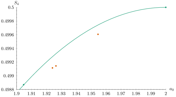
Figure 1: Fully-interacting fixed points for $N=4$.

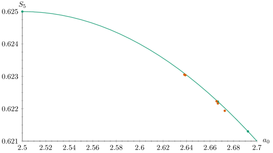
Figure 2: Fully-interacting fixed points for $N=5$. The leftmost point corresponds to $T_{5\pm}$ and the rightmost to $O(5)$.

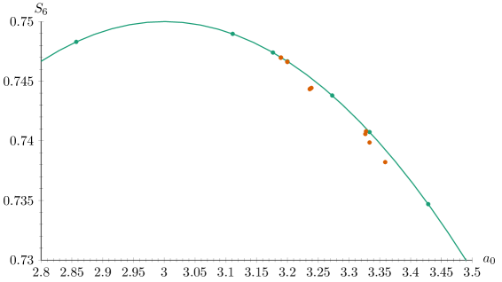
Figure 3: Fully-interacting fixed points for $N=6$. The leftmost point corresponds to $T_{6+}$ and the rightmost to $O(6)$.

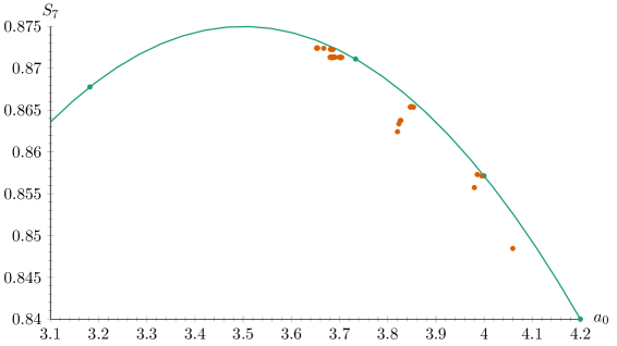
Figure 4: Fully-interacting fixed points for $N=7$. The leftmost point corresponds to $T_{7+}$ and the rightmost to $O(7)$.

6 Six Index Case

In $3-\varepsilon$ dimensions there may be fixed points starting from the renormalisable interaction $V(\phi)=\frac{1}{6!}\lambda_{ijklmn}\phi_{i}\phi_{j}\phi_{k}\phi_{l}\phi_{m}\phi_{n}$. At lowest order possible fixed points in the $\varepsilon$ expansion are determined, with a suitable rescaling, by finding solutions of

$$\lambda_{ijklmn}=S_{10,ijklmn}\,\lambda_{ijkpqr}\lambda_{lmnpqr}\,,$$ (6.1)

where $S_{n,ijklmn}$ here denotes the sum over the $n$ permutations, with unit weight, necessary to ensure the sum is fully symmetric in $ijklmn$. This is equivalent to

$$V(\phi)=\tfrac{1}{2}\,V_{ijk}(\phi)V_{ijk}(\phi)\,.$$ (6.2)

As before in (2.5) the coupling can be decomposed, with a similar notation for symmetrisation, as

$$\lambda_{ijklmn}=d_{0}\,S_{15,ijklmn}\,\delta_{ij}\delta_{kl}\delta_{mn}+S_{45,ijklmn}\,\delta_{ij}\delta_{kl}d_{2,mn}+S_{15,ijklmn}\,\delta_{ij}d_{4,klmn}+d_{6,ijklmn}\,,$$ (6.3)

for $d_{2},\,d_{4},d_{6}$ symmetric traceless tensors. With this expansion

$$a_{0}={} N(N+2)(N+4)d_{0}=\lambda_{iijjkk}\,,$$

$$a_{2}={} (N+4)^{2}(N+6)^{2}\,||d_{2}||^{2}=\lambda_{ijkkmm}\lambda_{ijllnn}-\tfrac{1}{N}\,a_{0}{\!}^{2}\,,$$

$$a_{4}={} (N+8)^{2}\,||d_{4}||^{2}=\lambda_{ijklmm}\lambda_{ijklnn}-\tfrac{6}{N+4}\,a_{2}-\tfrac{3}{N(N+2)}\,a_{0}{\!}^{2}\,,$$

$$||\lambda||^{2}={} \lambda_{ijklmn}\lambda_{ijklmn}=15N(N+2)(N+4)\,d_{0}{}^{2}+45(N+4)(N+6)\,||d_{2}||^{2}$$

$$\hskip 79.6678pt{}+15(N+8)\,||d_{4}||^{2}+||d_{6}||^{2}\,.$$ (6.4)

The fixed point equation (6.3), by contracting indices, requires

$$N(N+2)(N+4)d_{0}={} 6N(N+2)(N+4)(3N+22)d_{0}{}^{2}+36(N+4)(N+6)(N+11)||d_{2}||^{2}$$

$${}+6(N+8)(N+18)||d_{4}||^{2}+4\,||d_{6}||^{2}\,.$$ (6.5)

This requires

$$d_{0}\leqslant\tfrac{1}{6(3N+22)}\,.$$ (6.6)

Combining (6.4) and (6.5)

$$||\lambda||^{2} +\tfrac{3}{2}(N+8)^{2}\,||d_{4}||^{2}+9(N+4)(N+6)^{2}\,||d_{2}||^{2}$$

$$={} \tfrac{1}{288}\,N(N+2)-\tfrac{1}{2}N(N+2)\big{(}3(N+4)d_{0}-\tfrac{1}{12}\big{)}^{2}\leqslant\tfrac{1}{288}\,N(N+2)\,.$$ (6.7)

The constraint (6.6) does not here lead to any modification for low $N$.

For the $O(N)$ invariant theory, $\lambda_{ijklmn}=\lambda\,S_{15,ijklmn}\,\delta_{ij}\delta_{kl}\delta_{mn}$ or $V(\phi)=\tfrac{1}{48}\lambda(\phi^{2})^{3}$. At the fixed point solving (6.1) $\lambda=1/6(3N+22)$ and then (6.6) is saturated

$$d_{0}=\frac{1}{6(3N+22)}\,,\quad a_{2}=a_{4}=||d_{6}||^{2}=0\,,\qquad||\lambda||^{2}=\frac{5N(N+2)(N+4)}{12(3N+22)^{2}}\,.$$ (6.8)

For $N=1$, $||\lambda||^{2}=\tfrac{1}{100}$ so that without any decoupled free theories we expect $||\lambda||^{2}>\tfrac{1}{100}N$. For $N$ decoupled non free theories

$$||\lambda||^{2}=\tfrac{N}{100}\,,\ \ a_{0}=\tfrac{N}{10}\,,\ \ a_{2}=0\,,\ \ a_{4}=\tfrac{N(N-1)}{100(N+2)}\,,\ \ ||d_{6}||^{2}=\tfrac{N(N-1)(N-2)}{100(N+4)(N+8)}\,.$$ (6.9)

For $N\to\infty$ in the $O(N)$ case $||\lambda||^{2}\sim\tfrac{5}{108}N,\,a_{0}\sim\frac{1}{18}N^{2}$.

Assuming cubic symmetry $B_{N}$ there are just three couplings,

$$V_{C}(\phi)=\tfrac{1}{6!}\,g_{1}{\textstyle\sum_{i}}\,\phi_{i}{\!}^{6}+\tfrac{1}{48}\,g_{2}\,{\textstyle\sum_{i\neq j}}\,\phi_{i}{\!}^{4}\phi_{j}{\!}^{2}+\tfrac{1}{48}\,g_{3}\,{\textstyle\sum_{i\neq j\neq k}}\,\phi_{i}{\!}^{2}\phi_{j}{\!}^{2}\phi_{k}{\!}^{2}\,,$$ (6.10)

and

$$||\lambda||^{2}={} N\big{(}g_{1}{\!}^{2}+15(N-1)\,g_{2}{\!}^{2}+15(N-1)(N-2)\,g_{3}{\!}^{2}\big{)}\,,$$

$$a_{0}={} N\big{(}g_{1}+3(N-1)g_{2}+(N-1)(N-2)g_{3}\big{)}\,,\qquad a_{2}=0\,,$$

$$a_{4}={} \tfrac{N(N-1)}{N+2}\big{(}g_{1}+(N-7)g_{2}-3(N-2)g_{3}\big{)}^{2}\,,\quad a_{6}=\tfrac{N(N-1)(N-2)}{(N+4)(N+8))}\big{(}g_{1}-15g_{2}+30\big{)}^{2}\,,$$ (6.11)

The lowest order equations are just

$$g_{1}={} 10\,g_{1}{\!}^{2}+30(N-1)g_{2}{\!}^{2}\,,\quad g_{2}=4\,g_{1}g_{2}+36\,g_{2}{\!}^{2}+12(N-2)g_{2}g_{3}+18(N-2)g_{3}{\!}^{2}\,,$$

$$g_{3}={} 6\,g_{2}{\!}^{2}+36\,g_{2}g_{3}+6(3N-5)g_{3}{\!}^{2}\,.$$ (6.12)

This example was considered in [3], for $g_{1}/15=g_{2}/3=g_{3}=\lambda$ it reduces to the $O(N)$ case. For $N$ not very large there are three non trivial real solutions. Apart from the decoupled theory with $||\lambda||^{2}=\tfrac{1}{100}N$ there is the $O(N)$ symmetric fixed point and an irrational one with cubic symmetry. For $N=14$ these coincide so $N=14$ plays a similar role to $N=4$ in the four index case. For $N>14$ the cubic fixed point has higher $||\lambda||^{2}$. For $14034<N<14035$ there is a bifurcation point and for higher $N$ two new real fixed points, one of which is stable within this three coupling theory. In each case $||\lambda||^{2}\propto N$ for large $N$ where the different solutions for $g_{1}={\rm O}(1),\,g_{2}={\rm O}(N^{-\frac{1}{2}}),\,g_{3}={\rm O}(N^{-1})$ give

$$||\lambda||^{2}\sim\big{(}\tfrac{1}{100},\,\tfrac{5}{108},\,\tfrac{25}{448},\,\tfrac{25}{448},\,\tfrac{38}{675}\big{)}N\,.$$ (6.13)

Although not obviously required by (6.7) it appears in general that $||\lambda||^{2}\propto N$ for large $N$.

For the case of tetrahedral symmetry

$$V_{T}(\phi)=\tfrac{1}{48}\lambda(\phi^{2})^{3}+\tfrac{1}{48}g_{1}\,\phi^{2}{\textstyle\sum_{\alpha}}\,(\phi^{\alpha})^{4}+\tfrac{1}{72}g_{2}\,\big{(}{\textstyle\sum_{\alpha}}\,(\phi^{\alpha})^{3}\big{)}^{2}+\tfrac{1}{6!}g_{3}\,{\textstyle\sum_{\alpha}}\,(\phi^{\alpha})^{6}\,,$$ (6.14)

for

$$\phi^{\alpha}=\phi_{i}e_{i}{\!}^{\alpha}\,\ \alpha=1,\dots,N+1\,,\quad e_{i}{\!}^{\alpha}e_{i}{\!}^{\beta}=\delta^{\alpha\beta}-\tfrac{1}{N+1}\,,\ {\textstyle\sum_{\alpha}}e_{i}{\!}^{\alpha}=0\,,\ {\textstyle\sum_{\alpha}}e_{i}{\!}^{\alpha}e_{j}{\!}^{\alpha}=\delta_{ij}\,.$$ (6.15)

This has the symmetry group ${\cal S}_{N+1}\times{\mathbb{Z}}_{2}$. For $N=2$ only two couplings are necessary since the potential is invariant for $(\lambda,g_{1},g_{2},g_{3})\sim(\lambda-\mu-\frac{1}{2}\nu,g_{1}+2\mu,g_{2}-\nu,g_{3}+30\nu)$ while for $N=3,4$, $(\lambda,g_{1},g_{2},g_{3})\sim(\lambda-\frac{1}{2}\mu,g_{1}+3\mu,g_{2}+2\mu,g_{3}-60\mu)$ so the couplings reduce to three. When $N=3$ $V_{T}(\phi)$ is equivalent to $V_{C}(\phi)$.

The $O(N)$ invariants reduce to

$$||\lambda||^{2}={} 15N(N+2)(N+4)\lambda^{2}+\tfrac{30N}{N+1}\big{(}3N(N+4)g_{1}+4(N-1)g_{2}+\tfrac{N^{2}}{N+1}\,g_{3})\lambda,$$

$${}+15N\tfrac{N^{3}+1}{(N+1)^{3}}\big{(}(N+8)g_{1}+\tfrac{2N}{N+1}g_{3}\big{)}g_{1}+\tfrac{90N^{3}}{(N+1)^{2}}g_{1}{\!}^{2}$$

$${}+10N\tfrac{(N-1)^{2}}{(N+1)^{2}}\big{(}18g_{1}+(N+9)g_{2}+\tfrac{2N}{N+1}g_{3}\big{)}g_{2}+N\tfrac{N^{5}+1}{(N+1)^{5}}\,g_{3}{\!}^{2}\,,$$

$$a_{0}={} N(N+2)(N+4)\lambda+\tfrac{N}{N+1}\big{(}3N(N+4)g_{1}+4(N-1)g_{2}\big{)}+\tfrac{N^{3}}{(N+1)^{2}}\,g_{3}\,,\qquad a_{2}=0\,,$$

$$a_{4}={} \tfrac{N(N-1)(N-2)}{(N+1)^{3}(N+2)}\big{(}(N+1)(N+9)g_{1}+6Ng_{2}+Ng_{3}\big{)}^{2}\,.$$ (6.16)

The fixed point equations from (6.2) become

$$\lambda={} 6(3N+22)\lambda^{2}+6g_{1}{\!}^{2}+\tfrac{72}{N+1}(Ng_{1}-g_{2})\lambda-\tfrac{18(N-3)}{(N+1)^{2}}(g_{1}+g_{2})^{2}\,,$$

$$g_{1}={} (78g_{1}+36g_{2}+4g_{3})g_{1}+12\big{(}(N+18)g_{1}+6g_{2}+\tfrac{N}{N+1}g_{3}\big{)}\lambda-12\tfrac{N-1}{(N+1)^{2}}(g_{1}+g_{3})g_{2}$$

$${}+\tfrac{6}{N+1}\big{(}3(N-5)g_{2}{\!}^{2}-22g_{1}{\!}^{2}-40g_{1}g_{2}\big{)}\,,$$

$$g_{2}={} (N+16)g_{2}{\!}^{2}+72g_{1}g_{2}+120g_{2}\lambda-\tfrac{1}{N+1}\big{(}3(N+32)g_{1}{\!}^{2}+88g_{2}{\!}^{2}+180g_{1}g_{2}\big{)}$$

$${}+\tfrac{2N}{(N+1)^{2}}\big{(}(N-1)g_{2}-3g_{1}\big{)}g_{3}-\tfrac{1}{(N+1)^{3}}\,g_{3}{\!}^{2}\,,$$

$$g_{3}={} 30(N+32)g_{1}{\!}^{2}+1440g_{1}g_{2}+540g_{2}{\!}^{2}+10g_{3}{\!}^{2}+120g_{3}\lambda$$

$${}+\tfrac{60}{N+1}\big{(}(4N-3)g_{1}+3(N-1)g_{2}\big{)}g_{3}-\tfrac{30N}{(N+1)^{2}}\,g_{3}{\!}^{2}\,.$$ (6.17)

For $N=2,3$ the fixed points are identical to those for cubic symmetry. Apart from the $O(N)$ invariant fixed point at $N=4$ there is one tetrahedral fixed point and two tetrahedral fixed points are present for $N>4$. One of these collides with the $O(N)$ fixed point when $N=14$ and for higher $N$ has a larger $||\lambda||^{2}$. There are also bifurcation points for $319<N<320$, $507<N<508$, $14035<N<14036$ and $15695<N<15696$, where two new fixed points emerge.

The cubic and tetrahedral solutions all have $a_{2}=0$ reflecting the fact that there is just one quadratic invariant. More generally possibilities arise with just ${\cal S}_{N}$ symmetry which encompasses the cubic and tetrahedral cases but for which there are two quadratic invariants. Extending (3.4) in this case

$$\lambda_{iiiiii}=x_{1}\,,\quad\lambda_{iiiiij}=x_{2}\,,\quad\lambda_{iiiijj}=x_{3}\,,\quad\lambda_{iiiijk}=x_{4}\,,\quad\lambda_{iiijjj}=x_{5}\,,\quad\lambda_{iiijjk}=x_{6}$$

$$\lambda_{iiijkl}=x_{7}\,,\quad\lambda_{iijjkk}=x_{8}\,,\quad\lambda_{iijjkl}=x_{9}\,,\quad\lambda_{iijklm}=x_{10}\,,\quad\lambda_{ijklmn}=x_{11}\,,$$ (6.18)

with $i,j,k,l,m,n$ all different. The 11 couplings reduce to 9 for $N=4$ and 7 for $N=3$. The resulting potential with just $x_{1}=g_{1},\,x_{3}=g_{2},\,x_{8}=g_{3}$ non zero is identical to (6.10). As was the case with the four index case the $\beta$-function equations can be simplified by imposing $O(N-1)$ symmetry. This requires

$$5(x_{3}-x_{4})=x_{1}-x_{2}\,,\quad 2(x_{5}-x_{6})=4(x_{6}-x_{7})=x_{2}-x_{4}\,,\quad 3(x_{6}-x_{9})=2(x_{4}-x_{7})\,,$$

$$3(x_{8}-x_{9})=x_{3}-x_{6}\,,\quad 3x_{9}=2x_{10}+x_{6}\,,\quad 3x_{10}=2x_{11}+x_{7}\,,$$ (6.19)

leaving just four couplings. Defining

$$\sigma={} x_{1}+3(N-1)x_{3}+(N-1)(N-2)x_{8}\,,$$

$$\rho={} .x_{2}+(N-2)(\tfrac{1}{2}x_{4}+2x_{6})+\tfrac{1}{2}(N-2)(N-3)x_{9}\,,$$

$$\tau={} x_{1}+(N-7)x_{3}-3(N-2)x_{8}\,,\qquad\upsilon=x_{1}-15x_{3}+30x_{8}\,,$$ (6.20)

then along with (6.19)

$$a_{0}=N\sigma\,,\quad a_{2}=4(N-1)\rho^{2}\,,\quad a_{4}=\tfrac{N^{4}(N^{2}-1)}{4(N+2)(N+4)}\,\tau^{2}\,,\quad a_{6}=\tfrac{N^{6}(N^{2}-1)(N+3)}{256(N+4)(N+6)(N+8)}\,\upsilon^{2}\,,$$ (6.21)

the fixed point equations become

$$\sigma={} \tfrac{6(3N+22)}{(N+2)(N+4)}\,\sigma^{2}+\tfrac{144(N-1)(N+11)}{(N+4)(N+6)}\,\rho^{2}+\tfrac{3N^{3}(N^{2}-1)(N+18)}{2(N+2)(N+4)(N+8)}\,\tau^{2}+\tfrac{N^{5}(N^{2}-1)(N+3)}{64(N+4)(N+6)(N+8)}\,\upsilon^{2}\,,$$

$$\rho={} \big{(}\tfrac{24(N+11)}{(N+2)(N+4)}\,\sigma-\tfrac{18N^{3}(N+1)(N+14)}{(N+2)(N+4)^{2}(N+6)}\,\tau)\rho-\tfrac{N^{5}(N+1)(N+3)(N+18)}{16(N+4)(N+6)(N+8)^{2}}\,\tau\,\upsilon$$

$${}+\tfrac{12(N-2)(N^{2}+40N+264)}{(N+4)^{2}(N+6)}\,\rho^{2}+\tfrac{N^{3}(N-2)(N+1)(N^{2}+52N+432)}{4(N+4)^{2}(N+8)^{2}}\,\tau^{2}+\tfrac{N^{5}(N-2)(N+2)(N+3)}{128(N+6)(N+6)^{2}}\,\upsilon^{2}\,,$$

$$\tau={} \big{(}\tfrac{12(N+18)}{(N+2)(N+4)}\,\sigma+\tfrac{24(N^{2}-4)(N^{2}+52N+432)}{(N+4)^{2}(N+6)(N+8)}\,\rho\big{)}\tau-\tfrac{3N^{2}(N+2)(N+3)(N+18)}{(N+4)(N+6)^{2}(N+8)}\,\rho\,\upsilon$$

$${}+\tfrac{N^{3}(N^{2}-4)(N+3)(N+32)}{4(N+4)(N+6)(N+8)^{2}}\,\tau\,\upsilon$$

$${}-\tfrac{432(N+8)(N+14)}{(N+4)^{2}(N+6)^{2}}\,\rho^{2}-\tfrac{36N^{3}(N-2)(N+3)(N+14)}{(N+2)(N+4)^{2}(N+8)^{2}}\,\tau^{2}-\tfrac{3N^{5}(N-2)(N+3)(N+5)}{64(N+6)^{2}(N+8)^{2}}\,\upsilon^{2}\,,$$

$$\upsilon={} \big{(}\tfrac{120}{(N+2)(N+4)}\,\sigma+\tfrac{720(N-2)}{(N+6)(N+8)}\,\rho-\tfrac{90N^{3}(N-2)(N+5)}{(N+2)(N+6)(N+8)^{2}}\,\tau\big{)}\upsilon$$

$${}-\tfrac{2880(N+18)}{(N+4)(N+6)(N+8)}\,\rho\,\tau+\tfrac{120N(N-2)(N+32)}{(N+4)(N+8)^{2}}\,\tau^{2}+\tfrac{5N^{4}(N^{2}-4)(N+5)}{8(N+4)(N+6)(N+8)^{2}}\,\upsilon^{2}\,.$$ (6.22)

For low $N$ there is one non trivial solution in addition to the $O(N)$ symmetric one, this has higher $||\lambda||^{2}$ for $N>14$. For $206<N<207$ there is a bifurcation. For very large $N$ the solutions converge to the $O(N)$ symmetric fixed point.

6.1 Fixed Points for Low $N$

In a similar fashion to previously we have looked numerically snd analytically for fixed points for low $N$. For the values of $N$ considered here the fixed point with maximal $||\lambda||^{2}$ is always that with $O(N)$ symmetry as in (6.8).

$N=1$	$||\lambda||^{2}$	$a_{0}$	$a_{2}$	$a_{4}$	$a_{6}$	Symmetry	# different $\gamma$ and degeneracies	$\#{\kappa<0},\,{=0}$
$O_{1}$	$\tfrac{1}{100}$	$\tfrac{1}{10}$	0	0	0	${\mathbb{Z}}_{2}$	1(1)	$0,\,0$

$N=2$	$||\lambda||^{2}$	$a_{0}$	$a_{2}$	$a_{4}$	$a_{6}$	Symmetry	# different $\gamma$ and degeneracies	$\#{\kappa<0},\,{=0}$
$O_{2}$	$\tfrac{5}{196}$	$\tfrac{2}{7}$	0	0	0	$O(2)$	1(2)	$0,\,0$

(6.30)

For $N=4$

(6.51)

A pictorial representation of these fixed points (excluding the first one) is given in Figure 5. The distribution of these fixed points is similar to that of Figure 1 of the $d=4-\varepsilon$ case.

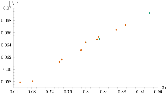
Figure 5: Fully-interacting fixed points for $N=4$ in $d=3-\varepsilon$.

For $N=5$ the number of solutions explode; those found by us are given in Appendix C.

7 Conclusion

The large number of potential fixed points which appear close together in the lowest order $\varepsilon$ expansion equations for $N=6$ and larger are presumably quite fragile. Reinstating $\varepsilon$, for two fixed points where $||\lambda_{1}-\lambda_{2}||=\xi\,\varepsilon$ at lowest order then what happens at higher orders in the $\varepsilon$ expansion for $\varepsilon\sim\xi$ is far from clear. In many of the examples obtained numerically $\xi\sim 10^{-3},10^{-4}$. Which fixed points survive in the interesting case when $\varepsilon=1$ is not at all apparent. In most cases, though perhaps not all, they can be understood in terms of perturbations of combinations of fixed point solutions for lower $N$. None of the solutions obtained here numerically saturate the bound (1.1) when the requirement that the fixed point is not a combination of decoupled fixed points is imposed.

Nevertheless there exist sporadic non trivial fixed point solutions which saturate the bound for higher $N$. These arise for $N=mn$, $m,n>1$, and there is a $O(m)\times O(n)/{\mathbb{Z}}_{2}$ symmetry with the scalar fields belonging to the bivector representation. These theories have a large $n$ limit [45]. There are just two couplings. Apart from $m=n=2$, where the fixed point is only $O_{4}$, the first real fixed point solution arises for $m=22,\,n=2$ where there are two fixed points having $S_{+}=\tfrac{6831}{1250},\,S_{-}=\tfrac{20328}{3721}$. When $m,n$ satisfy a certain diophantine equation the two fixed points present in general coincide and the bound is saturated. For this the integer solutions are obtained by $(m_{i+1},\,n_{i+1})=(10m_{i}-n_{i}+4,\,m_{i})$ and $m_{1}=7,\,n_{1}=1$ [1]. For $i\geqslant 4$, $m_{i}\approx\tfrac{3}{4}\,\alpha^{i},\ n_{i}\approx\tfrac{3}{4}\,\alpha^{i-1}$, $\alpha=5+\sqrt{24}$. Whether there are any other similar non trivial solutions satisfying the bound is unknown.

Unless strong symmetry conditions are imposed then for any $N\geqslant 6$ the stability matrix will have negative eigenvalues. This suggests according to standard lore that any phase transition is first order so that the apparent fixed point will not realise a CFT. Nevertheless the large numbers of solutions suggest that any classification of CFTs when $d=3$ for instance is likely to be very non trivial.

The discussion here is also incomplete in that an implicit assumption made is that the expansion involves only integer powers of $\varepsilon$ so that the lowest order contributions to the $\beta$-functions determine the leading contribution to the $\varepsilon$ expansion. This assumption breaks down near a bifurcation point [3]. However, the analysis may be potentially more complicated away from bifurcation points in that in some theories the $\beta$-function corresponding to one, or more, particular coupling is zero to lowest order in the loop expansion but is non zero at the next order. This situation can arise in large $N$ limits where couplings are rescaled by fractional powers of $N$. The expansion of the equations for a fixed point then typically involves $\sqrt{\varepsilon}$. As an illustration, for couplings $h,\,g_{a}$, $a=1,\dots,n$, then if to second order in a loop expansion the $\beta$-functions can be truncated to the form

$$\beta_{h}(h,g)={} k_{a}g_{a}\,h+k\,h^{3}+{\rm O}(g^{2}h)\,,$$

$$\beta_{a}(h,g)={} b_{a}(g)+\tfrac{1}{2}\,k_{a}\,h^{2}+c_{a}(g)h^{2}+{\rm O}(g^{3},g^{2}h^{2})\,,\quad b_{a}(g)={\rm O}(g^{2}),\,c_{a}(g)={\rm O}(g)\,,$$ (7.1)

assuming that at lowest order $\beta_{h}=\partial_{h}A,\,\beta_{a}=\partial_{a}A$ and also $\beta_{h}(-h,g)=-\beta_{h}(h,g)$, $\beta_{a}(-h,g)=\beta_{a}(h,g)$. Solving $\varepsilon\,h=\beta_{h}(h,g),\ \varepsilon\,g_{a}=\beta_{a}(h,g)$ neglecting cubic terms requires $h=0$ unless $g_{a}$ are constrained by $k_{a}g_{a}=\varepsilon$ and then, subject to this constraint, the $n$ equations $\varepsilon\,g_{a}=b_{a}(g)+\tfrac{1}{2}k_{a}\,h^{2}$ potentially determine $g_{a},\,h={\rm O}(\varepsilon)$, with the higher order terms generating the usual perturbative expansion in $\varepsilon$. However, if $k_{a}$ are zero, or can be scaled away in a large $N$ limit, we may take $h\sim h_{0}\,\varepsilon^{\frac{1}{2}},\,g_{a}={\rm O}(\varepsilon)$. The higher order terms then involve an expansion in powers of $\sqrt{\varepsilon}$. Similar scenarios arise in melonic theories [47, 48, 49]. The graphs relevant for the lowest order $\beta$-function in $\phi^{4}$ and $\phi^{6}$ theories may not be sufficient to generate the melonic interactions for fields with three or more indices.

The discussion of fixed points for the six index coupling undertaken in section 6 is less complete. All cases considered are such that $||\lambda||^{2}$ depends linearly on $N$ for large $N$ although there is no bound analogous to (1.1). Perhaps such a bound might follow from a more detailed analysis of the fixed point equations. The $O(N)$ symmetric fixed point is no longer the one with maximal $||\lambda||^{2}$ for $N>14$. However, the relevance to physical theories is tenuous.

Acknowledgments

This investigation started as part of a part III project in Natural Sciences in Cambridge with Igor Timofeev. His initial contributions involved the analysis of ${\cal S}_{N}$ symmetry and finding bounds in the six index case. We are grateful to the authors of [15] for sending us an early copy of their work. AS would like to thank Matthijs Hogervorst for valuable discussions and also sending a preliminary version of [21].

We are very grateful to Slava Rychkov who stimulated much of this work and who read this paper making many valuable suggestions.

This work has been partially supported by STFC consolidated grants ST/P000681/1, ST/T000694/1.

This research used resources provided by the Los Alamos National Laboratory Institutional Computing Program, which is supported by the U.S. Department of Energy National Nuclear Security Administration under Contract No. 89233218CNA000001. Research presented in this article was supported by the Laboratory Directed Research and Development program of Los Alamos National Laboratory under project number 20180709PRD1.

Appendix A Alternative Formulation

An index free notation due to Michel [17] is convenient in many cases for analysing the fixed point equation (2.1). For symmetric four index tensors $u_{ijkl},\,v_{ijkl}$, scalar products and symmetric tensor products defined by

$$u\cdot v=u_{ijkl}v_{ijkl}\,,\qquad(uv)_{ijkl}=u_{ijmn}v_{mnkl}\,,\quad(u\vee v)_{ijkl}=(P_{4}\cdot(uv))_{ijkl}\,,$$ (A.1)

for $P_{4}$ the projector onto symmetric four index tensors. Clearly $||v||^{2}=v\cdot v$ and the triple product $(u\vee v)\cdot w=u\cdot(v\vee w)$ is completely symmetric in $u,\,v,\,w$. $(v\vee v)_{iijj}=\tfrac{1}{3}(2||v||^{2}+v_{ijkk}v_{ijll})$ so that $v\vee v=0$ implies $v=0$. This product is commutative but not associative. Note that $(v\vee v)\vee(v\vee v)\neq v\vee(v\vee(v\vee v))$.

The fixed point and eigenvalue equations are then

$$3\,\lambda\vee\lambda=\lambda\,,\qquad 6\,\lambda\vee v=(\kappa+1)v\,.$$ (A.2)

The solutions $\{\kappa_{r},\,v_{r}\}$ can be chosen to form an orthonormal basis so that

$$v_{r}\cdot v_{s}=\delta_{rs}\,,\qquad\kappa_{0}=1\,,\quad v_{0}=\tfrac{1}{||\lambda||}\lambda\,.$$ (A.3)

In terms of this basis

$$3\,v_{r}\vee v_{s}={\textstyle\sum_{t}}\,C_{rst}\,v_{t}\,,\quad C_{rst}=3\,(v_{r}\vee v_{s})\cdot v_{t}=C_{(rst)}\,,\quad C_{rs0}=\tfrac{1}{2||\lambda||}(\kappa_{r}+1)\delta_{rs}\,.$$ (A.4)

Directly from (A.2)

$$\kappa+1=\tfrac{18}{||v||^{2}}\,(\lambda\vee\lambda)\cdot(v\vee v)=\tfrac{18}{||v||^{2}}\,(\lambda\lambda)\cdot P_{4}\cdot(vv)\geqslant 0\,.$$ (A.5)

Hence $\kappa\geqslant-1$.

A proof that $\kappa\leqslant 1$ in general is not immediately evident but should follow from bounds on the product. Using (A.2) twice

$$\tfrac{1}{36}(1-\kappa^{2})\,||v||^{2}=(\lambda\wedge\lambda)\cdot(v\wedge v)-(\lambda\wedge v)\cdot(\lambda\wedge v)$$

$${}=\tfrac{2}{3}\big{(}(\lambda\lambda)_{ijkl}(vv)_{ikjl}-(\lambda v)_{ijkl}(\lambda v)_{ikjl}\big{)}+\tfrac{1}{6}\big{(}(\lambda\lambda)_{ijkl}(vv)_{klij}-(\lambda v)_{ijkl}(\lambda v)_{klij}\big{)}\,.$$ (A.6)

For any symmetric matrices $A,B$, $\operatorname{tr}(A^{2}B^{2}-ABAB)=\tfrac{1}{2}\operatorname{tr}([A,B][B,A])\geqslant 0$ so that the second term is positive.

For $n$ decoupled theories where

$$3\,\lambda_{r}\vee\lambda_{s}=\delta_{rs}\,\lambda_{r}\,,\quad\lambda_{r}\cdot\lambda_{s}=0\,,\ \ r\neq s\,,\qquad r,s=1,\dots n\,,.$$ (A.7)

then with

$${\textstyle\sum_{r}}\,\lambda_{r}=\lambda,\,\quad v_{i}={\textstyle\sum_{r}}\,x_{i,r}\lambda_{r}\,,\quad{\textstyle\sum_{r}}\,x_{i,r}\,||\lambda_{r}||^{2}=0\,\quad{\textstyle\sum_{r}}\,x_{i,r}x_{j,r}\,||\lambda_{r}||^{2}=\delta_{ij}\,,$$ (A.8)

there are $n-1$ unit eigenvectors $v_{i}$, $i=1,\dots,n-1$, with $\kappa_{i}=1$, such that

$$3\,\lambda\vee v_{i}=v_{i}\,,\ \ \lambda\cdot v_{i}=0\,,\ \ v_{i}\cdot v_{j}=\delta_{ij}\,,\quad 3\,v_{i}\vee v_{j}=\delta_{ij}\,\tfrac{1}{||\lambda||^{2}}\,\lambda+{\textstyle\sum_{k}}\,C_{ijk}\,v_{k}\,,$$ (A.9)

where the symmetric tensor $C_{ijk}=\sum_{r}\,x_{i,r}x_{j,r}x_{k,r}||\lambda_{r}||^{2}$. Conversely finding eigenvectors satisfying (A.9) implies the presence of two or more decoupled theories. For $v_{0}=\lambda/||\lambda||$, and extending the index range for $i$ to $0,1,\dots,n-1$ with $x_{0,r}=1/||\lambda||$, then we may define $\lambda_{r}/||\lambda_{r}||=\sum_{i}\,x_{i,r}\,v_{i}$ where $\sum_{i}x_{i,r}\,x_{i,s}=\delta_{rs}/||\lambda_{r}||^{2}$. Crucially it is necessary to obtain (A.7) that $C_{ijk}=\sum_{r}\,x_{i,r}x_{j,r}x_{k,r}||\lambda_{r}||^{2}$ where $C_{0ij}=\delta_{ij}/||\lambda||$. Such a diagonalisation by essentially orthogonal matrices is not possible for arbitrary symmetric $C_{ijk}$ but depends on additional restrictions [50].

Appendix B Potentials and Symmetry Groups for $N=4$

In [24] various potentials corresponding to subgroups of $O(4)$ were identified. We revisit these from a different perspective. It is convenient here to adopt complex coordinates where $\varphi=\phi_{1}+i\phi_{2}$, $\psi=\phi_{3}+i\phi_{4}$.

First

$$V_{\rm dipentagonal}=\tfrac{1}{8}\lambda\big{(}|\varphi|^{2}+|\psi|^{2}\big{)}^{2}+\tfrac{1}{8}v\big{(}|\varphi|^{4}+|\psi|^{4}\big{)}+\tfrac{1}{48}i\,w\big{(}\varphi^{3}\psi+\varphi\,{\bar{\psi}}^{3}-{\bar{\varphi}}\,\psi^{3}-{\bar{\varphi}}^{3}{\bar{\psi}}\big{)}\,.$$ (B.1)

The symmetries which are subgroups of $O(4)$ are generated by

$$a:\ \big{(}\varphi,\,{\bar{\varphi}},\,\psi,\,{\bar{\psi}}\big{)}\to\big{(}e^{\frac{1}{5}\pi\,i}\varphi,\,e^{-\frac{1}{5}\pi\,i}{\bar{\varphi}},\,e^{-\frac{3}{5}\pi\,i}\psi,\,e^{\frac{3}{5}\pi\,i}{\bar{\psi}}\big{)}\,,$$

$$b:\ \big{(}\varphi,\,{\bar{\varphi}},\,\psi,\,{\bar{\psi}}\big{)}\to\big{(}i\,{\bar{\psi}},\,-i\,{\psi},\,i\,\varphi,\,-i\,{\bar{\varphi}}\big{)}\,,$$ (B.2)

where

$$a^{10}=b^{4}=e\,,\qquad b^{-1}a\hskip 0.5ptb=a^{3}\,.$$ (B.3)

Clearly $a\in{\mathbb{Z}}_{10}={\mathbb{Z}}_{5}\times{\mathbb{Z}}_{2},\,b\in{\mathbb{Z}}_{4}$ and $b$ generates the automorphisms of ${\mathbb{Z}}_{5}$. The symmetry group is then $({\mathbb{Z}}_{5}\rtimes{\mathbb{Z}}_{4})\times{\mathbb{Z}}_{2}$ with ${\mathbb{Z}}_{2}=\{e,\,a^{5}\}$. For $w=\pm 4v$ the symmetry is enhanced since

$$V_{\rm dipentagonal}\big{|}_{w=4v}=\tfrac{1}{8}(\lambda+2v)\big{(}\phi^{2})^{2}-\tfrac{5}{12}\,v\,{\textstyle\sum_{\alpha=1}^{5}}\big{(}\Phi^{\alpha})^{4}\,,$$ (B.4)

where

$$\Phi^{1}={} \tfrac{1}{2\sqrt{2}}\big{(}1+\tfrac{1}{\sqrt{5}}\big{)}\,\phi_{1}+\big{(}5+\sqrt{5}\big{)}^{-\frac{1}{2}}\,\phi_{2}+\tfrac{1}{2}\big{(}1+\tfrac{1}{\sqrt{5}}\big{)}^{\frac{1}{2}}\,\phi_{3}-\tfrac{1}{2\sqrt{2}}\big{(}1-\tfrac{1}{\sqrt{5}}\big{)}\,\phi_{4}\,,$$

$$\Phi^{2}={} \tfrac{1}{2\sqrt{2}}\big{(}1+\tfrac{1}{\sqrt{5}}\big{)}\,\phi_{1}-\big{(}5+\sqrt{5}\big{)}^{-\frac{1}{2}}\,\phi_{2}-\tfrac{1}{2}\big{(}1+\tfrac{1}{\sqrt{5}}\big{)}^{\frac{1}{2}}\,\phi_{3}-\tfrac{1}{2\sqrt{2}}\big{(}1-\tfrac{1}{\sqrt{5}}\big{)}\,\phi_{4}\,,$$

$$\Phi^{3}={} -\tfrac{1}{2\sqrt{2}}\big{(}1-\tfrac{1}{\sqrt{5}}\big{)}\,\phi_{1}-\tfrac{1}{2}\big{(}1+\tfrac{1}{\sqrt{5}}\big{)}^{\frac{1}{2}}\,\phi_{2}+\big{(}5+\sqrt{5}\big{)}^{-\frac{1}{2}}\,\phi_{3}+\tfrac{1}{2\sqrt{2}}\big{(}1+\tfrac{1}{\sqrt{5}}\big{)}\,\phi_{4}\,,$$

$$\Phi^{4}={} -\tfrac{1}{2\sqrt{2}}\big{(}1-\tfrac{1}{\sqrt{5}}\big{)}\,\phi_{1}+\tfrac{1}{2}\big{(}1+\tfrac{1}{\sqrt{5}}\big{)}^{\frac{1}{2}}\,\phi_{2}-\big{(}5+\sqrt{5}\big{)}^{-\frac{1}{2}}\,\phi_{3}+\tfrac{1}{2\sqrt{2}}\big{(}1+\tfrac{1}{\sqrt{5}}\big{)}\,\phi_{4}\,,$$

$$\Phi^{5}={} -\sqrt{\tfrac{2}{5}}\big{(}\phi_{1}+\phi_{4}\big{)}\,,$$ (B.5)

which are solutions of (3.31) for $N=4$. In terms of (B.2)

$$a:\ \big{(}\Phi^{1},\,\Phi^{2},\,\Phi^{3},\,\Phi^{4},\,\Phi^{5}\big{)}\to\big{(}-\Phi^{5},\,-\Phi^{4},\,-\Phi^{1},\,-\Phi^{3},\,-\Phi^{2}\big{)}\,,$$

$$b:\ \big{(}\Phi^{1},\,\Phi^{2},\,\Phi^{3},\,\Phi^{4},\,\Phi^{5}\big{)}\to\big{(}\Phi^{3},\,\Phi^{4},\,\Phi^{2},\,\Phi^{1},\,\Phi^{5}\big{)}\,,$$ (B.6)

but the full symmetry in (B.4) extends to ${\cal S}_{5}\times{\mathbb{Z}}_{2}$, with $a$ corresponding to a 5-cycle combined with a reflection and $b$ a $4$-cycle.

Secondly

$$V_{\rm orthotetragonal}={} \tfrac{1}{8}\lambda\big{(}|\varphi|^{2}+|\psi|^{2}\big{)}^{2}+\tfrac{1}{8}v\big{(}|\varphi|^{4}+|\psi|^{4}\big{)}+\tfrac{1}{48}w\big{(}\varphi^{2}\,{\bar{\psi}}^{2}+{\bar{\varphi}}^{2}\psi^{2}\big{)}$$

$${}+\tfrac{1}{48}i\,p(\varphi\,\psi^{3}+\varphi^{3}\psi-{\bar{\varphi}}^{3}{\bar{\psi}}-{\bar{\varphi}}\,{\bar{\psi}}^{3}\big{)}\,.$$ (B.7)

The symmetries are generated by

$$a:\ \big{(}\varphi,\,{\bar{\varphi}},\,\psi,\,{\bar{\psi}}\big{)}\to\big{(}e^{\frac{1}{4}\pi\,i}\varphi,\,e^{-\frac{1}{4}\pi\,i}{\bar{\varphi}},\,e^{\frac{5}{4}\pi\,i}\psi,\,e^{-\frac{5}{4}\pi\,i}{\bar{\psi}}\big{)}\,,$$

$$b:\ \big{(}\varphi,\,{\bar{\varphi}},\,\psi,\,{\bar{\psi}}\big{)}\to\big{(}e^{\frac{1}{4}\pi\,i}{\bar{\varphi}},\,e^{-\frac{1}{4}\pi\,i}\varphi,\,e^{\frac{1}{4}\pi\,i}{\bar{\psi}},\,\,e^{-\frac{1}{4}\pi\,i}\psi\big{)}\,,$$

$$c:\ \big{(}\varphi,\,{\bar{\varphi}},\,\psi,\,{\bar{\psi}}\big{)}\to\big{(}\psi,\,{\bar{\psi}},\,\varphi,\,{\bar{\varphi}}\big{)}\,,$$ (B.8)

with

$$a^{8}=b^{2}=c^{2}=e\,,\qquad b\hskip 0.5ptc\hskip 0.5ptb=c\,,\qquad b\hskip 0.5pta\hskip 0.5ptb=a^{7}\,,\qquad c\hskip 0.5pta\hskip 0.5ptc=a^{5}\,.$$ (B.9)

where $a\in{\mathbb{Z}}_{8},\,b,c\in{\mathbb{Z}}_{2}$. $b,c$ generate ${\rm Aut}({\mathbb{Z}}_{8})={\mathbb{Z}}_{2}\times{\mathbb{Z}}_{2}$ and the symmetry group is ${\mathbb{Z}}_{8}\rtimes({\mathbb{Z}}_{2}\times{\mathbb{Z}}_{2})$.

For a potential containing cubic symmetry

$$V_{\rm trigonal\,cubic}={} \tfrac{1}{8}\lambda\big{(}\phi^{2}\big{)}^{2}+\tfrac{1}{24}v\big{(}\phi_{1}{\!}^{4}+\phi_{2}{\!}^{4}+\phi_{3}{\!}^{4}+\phi_{4}{\!}^{4}\big{)}$$

$$\hskip-14.22636pt{}+\tfrac{1}{24}\,w\big{(}\phi_{1}\phi_{2}(\phi_{3}{\!}^{2}-\phi_{4}{\!}^{2})-\phi_{2}\phi_{3}(\phi_{4}{\!}^{2}-\phi_{1}{\!}^{2})-\phi_{3}\phi_{4}(\phi_{1}{\!}^{2}-\phi_{2}{\!}^{2})-\phi_{4}\phi_{1}(\phi_{2}{\!}^{2}-\phi_{3}{\!}^{2})$$

$$\qquad{}+\phi_{1}\phi_{3}(\phi_{2}{\!}^{2}-\phi_{4}{\!}^{2})-\phi_{2}\phi_{4}(\phi_{3}{\!}^{2}-\phi_{1}{\!}^{2})\big{)}\,.$$ (B.10)

The symmetry group is a subgroup of the permutations and reflections comprising the cubic symmetry group $B_{4}$ and is generated by

$$\hskip-8.5359ptx:\ (\phi_{1},\phi_{2},\phi_{3},\phi_{4})\to(-\phi_{3},\phi_{4},\phi_{1},-\phi_{2})\,,\quad y:\ (\phi_{1},\phi_{2},\phi_{3},\phi_{4})\to(\phi_{2},-\phi_{1},\phi_{4},-\phi_{3})\,,$$

$$\hskip-8.5359pta:\ (\phi_{1},\phi_{2},\phi_{3},\phi_{4})\to(\phi_{1},-\phi_{4},-\phi_{2},\phi_{3})\,,\quad b:\ (\phi_{1},\phi_{2},\phi_{3},\phi_{4})\to(-\phi_{1},-\phi_{4},\phi_{3},-\phi_{2})\,,$$ (B.11)

where

$$x^{4}=y^{4}=a^{3}=b^{2}=e\,,\quad x^{2}=y^{2}\,,\quad y\hskip 0.5ptx\hskip 0.5pty^{-1}=x^{-1}\,,\quad b\hskip 0.5pta\hskip 0.5ptb=a^{2}\,,$$

$$b\hskip 0.5ptx\hskip 0.5ptb=x^{3}\,,\quad b\hskip 0.5pty\hskip 0.5ptb=x\hskip 0.5pty\,,\quad a\hskip 0.5ptx\hskip 0.5pta^{-1}=y\,,\quad a\hskip 0.5pty\hskip 0.5pta^{-1}=x\,.$$ (B.12)

$x,\,y$ generate the quaternion group ${\rm Q}_{8}$ and $a,b$, ${\cal S}_{3}<{\rm Aut}({\rm Q}_{8})$ and the symmetry group is then ${\rm Q}_{8}\rtimes{\cal S}_{3}$.

For the remaining case with diorthorhombic symmetry the symmetry group is obtained by combining two 2-cycles with reflections and can be generated by

$$\hskip-8.5359pta:\ (\phi_{1},\phi_{2},\phi_{3},\phi_{4})\to(-\phi_{2},\phi_{1},-\phi_{4},\phi_{3})\,,\quad r:\ (\phi_{1},\phi_{2},\phi_{3},\phi_{4})\to(-\phi_{1},\phi_{2},-\phi_{3},\phi_{4})\,,$$

$$\hskip-8.5359pts:\ (\phi_{1},\phi_{2},\phi_{3},\phi_{4})\to(\phi_{4},-\phi_{3},-\phi_{2},\phi_{1})\,,\quad t:\ (\phi_{1},\phi_{2},\phi_{3},\phi_{4})\to(\phi_{1},-\phi_{2},-\phi_{3},\phi_{4})\,,$$ (B.13)

where

$$a^{4}=r^{2}=s^{2}=t^{2}=e\,,\quad r\hskip 0.5pta\hskip 0.5ptr=a^{3}\,,\ s\hskip 0.5ptt=t\hskip 0.5pts\,,\ s\hskip 0.5pta\hskip 0.5pts=a\,,\ s\hskip 0.5ptr\hskip 0.2pts=ra^{2}\,,\ t\hskip 0.5pta\hskip 0.5ptt=a^{3}\,,\ t\hskip 0.5pts\hskip 0.5ptt=s\,.$$ (B.14)

The symmetry group is then $D_{4}\rtimes({\mathbb{Z}}_{2}\times{\mathbb{Z}}_{2})$.

Appendix C Results for Six Indices and $N=5$

$N=5$	$||\lambda||^{2}$	$a_{0}$	$a_{2}$	$a_{4}$	$a_{6}$	Symmetry	# different $\gamma$ and degeneracies	$\#{\kappa<0},\,{=0}$
Tetrahedral	0.059928	0.60697	0	0.029631	0.008195	${\cal S}_{6}\times{\mathbb{Z}}_{2}$	1(5)	$180,\,10$
	0.086604	1.13032	0.001295	0.020277	0.001779		5(1,1,1,1,1)	$161,\,10$
	0.086786	1.13087	0.001470	0.020024	0.002115		5(1,1,1,1,1)	$160,\,10$
	0.086897	1.14497	0.002557	0.018825	0.001587		5(1,1,1,1,1)	$161,\,10$
	0.086907	1.13058	0.000499	0.020599	0.002045		2(1,4)	$159,\,10$
	0.086979	1.14649	0.002464	0.018787	0.001589		5(1,1,1,1,1)	$160,\,10$
	0.086985	1.14824	0.003249	0.018207	0.001715		5(1,1,1,1,1)	$160,\,10$
	0.087111	1.15711	0.003759	0.017509	0.001442		5(1,1,1,1,1)	$159,\,10$
	0.087490	1.16241	0.002244	0.018096	0.001248		5(1,1,1,1,1)	$159,\,10$
	0.087604	1.17008	0.002640	0.017501	0.001016		5(1,1,1,1,1)	$159,\,10$
	0.087637	1.17227	0.003587	0.016773	0.001215		5(1,1,1,1,1)	$158,\,10$
	0.087754	1.16267	0.001418	0.018462	0.001436		4(1,1,1,2)	$159,\,10$
	0.088058	1.17617	0.003603	0.016345	0.001685		5(1,1,1,1,1)	$158,\,10$
	0.088081	1.16953	0.000824	0.018411	0.001328		3(2,2,1)	$159,\,10$
	0.088285	1.17785	0.001260	0.017697	0.001229		5(1,1,1,1,1)	$158,\,10$
	0.088292	1.17337	0.000824	0.018139	0.001425		5(1,1,1,1,1)	$160,\,10$
	0.088293	1.17361	0.000863	0.018105	0.001422		5(1,1,1,1,1)	$159,\,10$
	0.088304	1.17498	0.001204	0.017822	0.001451		5(1,1,1,1,1)	$158,\,10$
	0.088322	1.17327	0.000940	0.018046	0.001522		3(2,2,1)	$159,\,10$
	0.088362	1.17530	0.001145	0.017813	0.001511		5(1,1,1,1,1)	$159,\,10$
	0.0883660	1.17522	0.001074	0.017860	0.001502		5(1,1,1,1,1)	$158,\,10$
	0.0883661	1.17554	0.000756	0.018060	0.001379		4(1,2,1,1)	$158,\,10$
	0.088368	1.17526	0.001010	0.017899	0.001483		4(1,2,1,1)	$157,\,10$
	0.088373	1.17742	0.001607	0.017423	0.001525		5(1,1,1,1,1)	$158,\,10$
	0.088407	1.17794	0.000685	0.017996	0.001256		4(2,1,1,1)	$157,\,10$
	0.088436	1.17880	0.000948	0.017771	0.001330		4(1,2,1,1)	$159,\,10$
	0.088438	1.17952	0.001025	0.017693	0.001306		5(1,1,1,1,1)	$158,\,10$
	0.088486	1.18006	0.001868	0.017080	0.001618		5(1,1,1,1,1)	$158,\,10$
	0.088489	1.18148	0.002051	0.016905	0.001580		5(1,1,1,1,1)	$157,\,10$
	0.088497	1.18007	0.001816	0.017107	0.001620		5(1,1,1,1,1)	$157,\,10$
	0.088828	1.18761	0.000364	0.017581	0.001215		5(1,1,1,1,1)	$158,\,10$
	0.088834	1.18810	0.000343	0.017573	0.001183		5(1,1,1,1,1)	$157,\,10$
	0.088922	1.19024	0.000733	0.017174	0.001311		4(1,1,1,2)	$157,\,10$
	0.088924	1.18914	0.000503	0.017367	0.001321		5(1,1,1,1,1)	$156,\,10$
	0.089025	1.19268	0.000427	0.017218	0.001227		3(1,2,2)	$156,\,10$
	0.089050	1.19471	0.000993	0.016747	0.001308		5(1,1,1,1,1)	$156,\,10$
	0.089405	1.20459	0.000711	0.016313	0.001161		5(1,1,1,1,1)	$155,\,10$
	0.089658	1.21752	0.001131	0.015335	0.000861		5(1,1,1,1,1)	$156,\,10$
	0.089664	1.21837	0.001347	0.015151	0.000883		5(1,1,1,1,1)	$155,\,10$
	0.089809	1.22199	0.001082	0.015078	0.000812		5(1,1,1,1,1)	$156,\,10$
	0.089812	1.22241	0.001163	0.015003	0.000816		5(1,1,1,1,1)	$155,\,10$
	0.089829	1.22319	0.001236	0.014910	0.000816		5(1,1,1,1,1)	$155,\,10$
	0.089836760	1.2236759	0.001227	0.0148897	0.0007946		5(1,1,1,1,1)	$155,\,10$
	0.089836763	1.2236756	0.001228	0.0148892	0.0007949		5(1,1,1,1,1)	$154,\,10$
	0.089853	1.22183	0.001188	0.014984	0.000934		4(1,1,1,2)	$154,\,10$
	0.089874	1.22602	0.001784	0.014392	0.000879		5(1,1,1,1,1)	$153,\,10$
	0.089891	1.22504	0.001058	0.014907	0.000747		4(1,1,1,2)	$153,\,10$
	0.090085	1.22324	0.000673	0.015112	0.001088		4(1,2,1,1)	$154,\,10$
$S_{5}$	0.090280	1.20824	0.000040	0.016030	0.002249		2(1,4)	$156,\,10$
Tetrahedral	0.090282	1.20657	0	0.016123	0.002354	$\mathcal{S}_{6}\times\mathbb{Z}_{2}$	1(5)	$155,\,10$
$S_{5}$	0.090331	1.22279	0.000387	0.014936	0.001123		2(1,4)	$155,\,10$
	0.090333	1.22305	0.000406	0.015133	0.001457		4(1,2,1,1)	$155,\,10$
	0.090335	1.22388	0.000391	0.015106	0.001400		4(1,1,1,2)	$155,\,10$
	0.090336	1.22408	0.000407	0.015087	0.001393		5(1,1,1,1,1)	$154,\,10$
	0.0903408	1.22873	0.000484	0.014829	0.001116		4(1,2,1,1)	$154,\,10$
	0.09034186	1.22880	0.000474	0.014832	0.001110		4(1,1,1,2)	$154,\,10$
	0.09034189	1.22881	0.000477	0.014830	0.001111		5(1,1,1,1,1)	$153,\,10$
	0.09034793	1.22925	0.000611	0.014716	0.001134		4(1,1,2,1)	$153,\,10$
	0.09034799	1.22959	0.000609	0.014703	0.001111		4(1,1,2,1)	$152,\,10$
	0.090349	1.22981	0.000650	0.014665	0.001112		3(1,3,1)	$152,\,10$
	0.090400	1.21586	0.000240	0.015504	0.002006		2(4,1)	$154,\,10$
	0.090433	1.23571	0.001065	0.014069	0.001002		3(1,1,3)	$152,\,10$
	0.0904737	1.22328	0.000210	0.015160	0.001628		2(3,2)	$154,\,10$
	0.0904742	1.22430	0.000351	0.015022	0.001605		3(3,1,1)	$154,\,10$
	0.090482	1.22470	0.000301	0.015033	0.001577		4(2,1,1,1)	$153,\,10$
	0.090507	1.22593	0.000381	0.014909	0.001564		4(1,2,1,1)	$153,\,10$
$S_{5}$	0.090534	1.24451	0.001430	0.013355	0.000722		2(1,4)	$151,\,10$
	0.090595883	1.235964	0.0007011	0.0141916	0.001159		5(1,1,1,1,1)	$152,\,10$
	0.090595889	1.235956	0.0007014	0.0141918	0.001160		4(1,2,1,1)	$151,\,10$
	0.090613	1.24187	0.001398	0.013446	0.001024		5(1,1,1,1,1)	$153,\,10$
	0.090707	1.23593	0.000565	0.014210	0.001316		3(1,2,2)	$153,\,10$
	0.090712	1.23681	0.000661	0.014102	0.001297		5(1,1,1,1,1)	$152,\,10$
	0.090760	1.24918	0.001474	0.012955	0.000835		5(1,1,1,1,1)	$152,\,10$
	0.090794	1.24541	0.001198	0.013294	0.001051		5(1,1,1,1,1)	$153,\,10$
	0.090795	1.24513	0.001188	0.013313	0.001067		5(1,1,1,1,1)	$152,\,10$
	0.090804	1.24404	0.001021	0.013469	0.001102		5(1,1,1,1,1)	$152,\,10$
	0.090813	1.24536	0.001108	0.013343	0.001060		5(1,1,1,1,1)	$151,\,10$
	0.090823	1.25279	0.001705	0.012586	0.000788		4(1,1,2,1)	$151,\,10$
	0.090844	1.24470	0.001067	0.013381	0.001144		5(1,1,1,1,1)	$152,\,10$
	0.090849	1.24569	0.001190	0.013249	0.001129		5(1,1,1,1,1)	$151,\,10$
	0.090850	1.24582	0.001214	0.013227	0.001129		5(1,1,1,1,1)	$151,\,10$
	0.090862	1.24704	0.001341	0.013076	0.001112		5(1,1,1,1,1)	$150,\,10$
	0.090904	1.25430	0.001693	0.012467	0.000832		5(1,1,1,1,1)	$152,\,10$
	0.090909	1.25468	0.001740	0.012414	0.000831		5(1,1,1,1,1)	$151,\,10$
	0.090940	1.25472	0.001923	0.012270	0.000940		5(1,1,1,1,1)	$151,\,10$
	0.090944	1.25487	0.001938	0.012250	0.000943		5(1,1,1,1,1)	$150,\,10$
	0.091096	1.25570	0.002404	0.011797	0.001307		4(1,1,2,1)	$149,\,10$
	0.091113	1.26449	0.003398	0.010689	0.001095		3(2,2,1)	$151,\,8$
	0.091432	1.26389	0.000905	0.012169	0.000913		3(2,1,2)	$150,\,9$
	0.091764	1.28127	0.001267	0.010812	0.000540		3(2,2,1)	$151,\,9$
	0.091790	1.28346	0.001458	0.010550	0.000512		3(1,2,2)	$150,\,10$
	0.091908	1.28365	0.001213	0.010625	0.000633		5(1,1,1,1,1)	$149,\,10$
	0.091949	1.28351	0.001121	0.010666	0.000684		5(1,1,1,1,1)	$148,\,10$
	0.092077	1.29365	0.002008	0.009439	0.000582		5(1,1,1,1,1)	$147,\,10$
	0.092297	1.29283	0.000808	0.010138	0.000641		4(1,2,1,1)	$148,\,9$
	0.092329	1.29725	0.001581	0.009357	0.000677		5(1,1,1,1,1)	$146,\,10$
	0.092398	1.29378	0.000012	0.010550	0.000512		2(4,1)	$151,\,8$
	0.092407	1.29236	0.000034	0.010606	0.000621		4(1,2,1,1)	$149,\,9$
	0.0924161	1.29074	0.000054	0.010676	0.000739		3(2,1,2)	$147,\,10$
	0.0924165	1.29201	0.000007	0.010638	0.000649		2(2,3)	$148,\,9$
	0.092432	1.29016	0.000042	0.010705	0.000799		3(1,3,1)	$146,\,10$
Cubic	0.092476	1.28936	0	0.010747	0.000911	$B_{5}$	1(5)	$145,\,10$
	0.092925	1.31105	0.000589	0.008836	0.000612		2(1,4)	$145,\,10$
	0.092939	1.30896	0.000614	0.008931	0.000766		2(1,4)	$144,\,10$
	0.092986	1.32144	0.000475	0.008258	0.000090		2(1,4)	$146,\,8$
	0.093047	1.32271	0.000643	0.008029	0.000178		3(2,1,2)	$146,\,8$
	0.093258	1.32803	0.001126	0.007244	0.000404		4(2,1,1,1)	$144,\,9$
	0.093473	1.33092	0.001014	0.006999	0.000587		2(2,3)	$143,\,9$
	0.094124	1.35768	0.001065	0.004824	0.000298		2(3,2)	$142,\,7$
$S_{5}$	0.094738	1.37896	0.000936	0.003056	0.000237	$O(4)$	2(4,1)	$141,\,4$
$O_{5}$	$\frac{525}{5476}$	$\frac{105}{74}$	0	0	0	$O(5)$	1(5)	$140,\,0$

A pictorial representation of these fixed points (excluding the first one) is given in Figure 6. The distribution of fixed points in $d=3-\varepsilon$ is similar to that of Figure 1 of the $d=4-\varepsilon$ case.

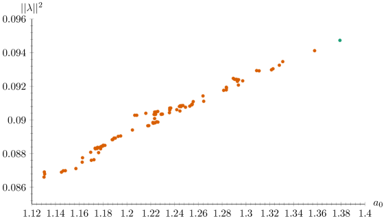
Figure 6: Fully-interacting fixed points for $N=5$ in $d=3-\varepsilon$.