Learning as Abduction:
Trainable Natural Logic Theorem Prover for Natural Language Inference

Abstract

Tackling Natural Language Inference with a logic-based method is becoming less and less common. While this might have been counterintuitive several decades ago, nowadays it seems pretty obvious. The main reasons for such a conception are that (a) logic-based methods are usually brittle when it comes to processing wide-coverage texts, and (b) instead of automatically learning from data, they require much of manual effort for development. We make a step towards to overcome such shortcomings by modeling learning from data as abduction: reversing a theorem-proving procedure to abduce semantic relations that serve as the best explanation for the gold label of an inference problem. In other words, instead of proving sentence-level inference relations with the help of lexical relations, the lexical relations are proved taking into account the sentence-level inference relations. We implement the learning method in a tableau theorem prover for natural language and show that it improves the performance of the theorem prover on the sick dataset by $1.4\%$ while still maintaining high precision ($>94\%$). The obtained results are competitive with the state of the art among logic-based systems.

1 Introduction

Natural language inference (NLI) is a well-established task for measuring intelligent systems’ capacity of natural language understanding Cooper et al. (1996); Dagan et al. (2005). To improve and better evaluate the systems on the NLI task, many annotated NLI datasets are prepared and used for training and evaluating NLP models. Generally speaking, an NLI dataset is a set of natural language sentence pairs, called premise-hypothesis pairs, that are annotated by crowd workers with one of three inference labels (entailment, contradiction, and neutral), representing a semantic relation from a premise to a hypothesis.

Currently, the state-of-the-art systems in NLI are exclusively based on Deep Learning (DL). One of the reasons for this is that DL-based systems can eagerly learn from task-related data and also take an advantage form high-quality pre-trained word embeddings. The training phase helps them to obtain competitive scores on the in-domain test part. On the other hand, logic-based systems are becoming less favored for NLI since it is hard to scale them up for reasoning with wide-coverage sentences. Despite some rare exceptions Martínez-Gómez et al. (2017); Yanaka et al. (2018), it is notoriously hard to effectively and efficiently train logic-based systems on NLI datasets.

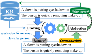
Figure 1: Theorem proving retrieves necessary semantic relations from KB, e.g., eyeshadow is make-up. To learn domain-specific relations, e.g., put on is incompatible with remove (not found in KB), abduction reverse proves semantic relations from training samples.

Although DL-based systems are more robust than logic-based ones, the latter systems offer unique virtues such as a transparent reasoning procedure and reasoning with multiple premises. An opaque decision procedure of DL-based systems makes it difficult to estimate a share of knowledge from what was learned by the systems, because not all what is learned is knowledge. Behind high performance of DL-based systems on particular NLI datasets, one might miss the systems’ inability of generalization Glockner et al. (2018) or the exploitation of annotation artefacts Poliak et al. (2018); Gururangan et al. (2018).

In this paper, we are not comparing logic- and DL-based approaches with respect to the NLI task. Rather, we are proposing a learning method which demonstrates how a logic-based NLI system can be trained on NLI dataset, the aspect in which DL approaches to NLI significantly outperform symbolic approaches. The proposed learning algorithm is inspired by abductive reasoning, which is often referred to as inference to the best explanation. Following the abduction, the algorithm allows learning those semantic relations over words and short phrases that best explain gold inference labels of NLI problems (see Figure 1). In this way, the current work contributes to automated knowledge acquisition from data, which is considered as a major issue in NLI (Dagan et al., 2013, p. 7).

The paper makes contributions along two lines: (a) describing how learning as abduction enables a trainable theorem prover for NLI, and (b) implementing the algorithm and evaluating its effectiveness. The original aspect of the research is the conceptual simplicity of the learning algorithm. In particular, the standard workflow of the logic-based theorem prover is reversed: instead of proving sentence-level inference relations with the help of lexical relations, the lexical relations are proved taking into account the sentence-level inference relations. Throughout the paper we answer the following research questions:

1. What is a computationally feasible learning method that allows training the natural language theorem prover on NLI problems?

2. How can learning pseudo-knowledge be avoided?

3. Can the learned knowledge replace the lexical knowledge database like WordNet?

4. To what extent the learned knowledge boosts the performance of the prover?

The rest of the paper briefly introduces the natural language theorem prover (Section 2), describes the new learning algorithm motivated by abduction (Section 3), outlines settings of experiments (Section 4), reports and analyzes results of the experiments (Section 5 and Section 6), overviews related work and compares it with the current one (Section 7), and finally, concludes the paper by answering the research questions (Section 8).

2 Natural Language Theorem Prover

For our experiments, we employ a natural language theorem prover, called LangPro Abzianidze (2017a), which is an implementation of Natural Tableau—an analytic tableau system for natural logic Muskens (2010); Abzianidze (2017b). An inference procedure is more central to Natural Tableau and its prover than it is usually for other logic-based NLI systems Bos and Markert (2005); Mineshima et al. (2015), which first derives meaning representations and then uses a proof engine for inference. The inference in Natural Tableau not only helps to prove semantic relations but also further expands semantics of logical forms (e.g., shifting from higher to lower-order terms). This makes it difficult to separate inference and semantic representations in Natural Tableau. Its central role of inference makes LangPro a suitable candidate for the data-driven learning experiment based on automated theorem proving.

baseline,for tree=align=center, parent anchor=south, child anchor=north, l sep=4.5mm, s sep=20mm [  $\textbf{{a}}~{}\textbf{{hedgehog}}~{}(\textbf{{be}}~{}(\lambda x.\,\textbf{{a}}~{}\textbf{{boy}}~{}(\lambda y.\,\textbf{{by}}~{}y~{}\textbf{{cradle}}~{}x))):\mathbb{T}$
 $\textbf{{a}}~{}\textbf{{person}}~{}(\lambda x.\,\textbf{{an}}~{}\textbf{{animal}}~{}(\lambda y.\,\textbf{{hold}}~{}y~{}x):\mathbb{F}$ [  $\textbf{{hedgehog}}:[h]:\mathbb{T}$
 $\textbf{{a}}~{}\textbf{{boy}}~{}(\lambda y.\,\textbf{{by}}~{}y~{}\textbf{{cradle}}~{}h):\mathbb{T}$, labelA= [1] , [  $\textbf{{boy}}:[b]:\mathbb{T}$
 $\textbf{{by}}~{}b~{}\textbf{{cradle}}:[h]:\mathbb{T}$, labelA= [4] , [  $\textbf{{cradle}}:[h,b]\mathbb{T}$, labelA= [6] , labB=0mm [2,$b$] [  $\textbf{{person}}:[b]:\mathbb{F}$ [ $\times$ , labelA= [5,8] ] ] [  $\textbf{{an}}~{}\textbf{{animal}}~{}(\lambda y.\,\textbf{{hold}}~{}y~{}b):\mathbb{F}$, labB=0mm [9,$h$] [  $\textbf{{animal}}:[h]:\mathbb{F}$ [ $\times$ , labelA= [3,10] ] ] [  $\textbf{{hold}}:[h,b]:\mathbb{F}$ [ $\times$ , labelA= [7,11] ] ] ] ] ] ] ]

Figure 2: On the left, a closed tableau which proves the entailment relation by failing to refute it. On the right, a set of inference rules that help to unfold semantics of larger terms.

The logic behind Natural Tableau and the prover is a higher-order logic (aka simple type theory) which also acts as a version of natural logic van Benthem (2008); Moss (2010). The $\lambda$-terms, given below with their corresponding sentences, represent logical forms of the natural logic.

A hedgehog is cradled by a boy (1)

$$\textbf{{a}}~{}\textbf{{hedgehog}}\,\big{(}\textbf{{be}}\,(\lambda x.\,\textbf{{a}}~{}\textbf{{boy}}\,(\lambda y.\,\textbf{{by}}\,y\,\textbf{{cradle}}\,x))\big{)}\kern-8.53581pt$$ (1a)

A person holds an animal (2)

$$\textbf{{a}}~{}\textbf{{person}}~{}(\lambda x.\,\textbf{{an}}~{}\textbf{{animal}}~{}(\lambda y.\,\textbf{{hold}}~{}y~{}x))$$ (2a)

Most dogs which jumped also barked loud (3)

$$\textbf{{most}}~{}(\textbf{{which}}~{}\textbf{{jump}}~{}\textbf{{dog}})~{}\big{(}\textbf{{also}}~{}(\textbf{{loud}}~{}\textbf{{bark}})\big{)}$$ (3a)

In addition to the lexical terms, the terms employ only variables and constants. Therefore, common logical connectives (e.g., $\wedge$, $\neg$) and quantifiers (e.g., $\exists$, $\forall$) are not part of the formal language. The terms are built using the $\lambda$ abstraction and function application. The role of variables and $\lambda$ is to access and fill certain argument positions and control scope. Variables and $\lambda$ are mainly used for terms with arity two or more, like cradle and hold. Abzianidze (2015) showed that the terms can be automatically obtained from the derivations of Combinatory Categorial Grammar (CCG, Steedman, 2000). Since the workflow for the theorem proving is important to understand the proposed learning algorithm, we demonstrate on the example how inference problems are solved by the prover.

After the sentences of an NLI problem are parsed with a parser and converted into $\lambda$-terms, the natural tableau prover verifies the problem on entailment and contradiction relations. For example, to prove that (1) entails (2), the tableau prover searches for a situation that makes (1a) true and (2a) false. In other words, it attempts to build a counterexample model that refutes the entailment relation. In Section 2, the proof tree, so-called tableau, depicts the search for the counterexample.

The tableau starts with (1a) being true and (2a) false, expressed by the entries and . But what are the meanings of and ? To flesh out their meanings, inference rules are applied to the entries. In particular, produces and with the help of the rule ($\exists_{\mathbb{T}}$), which says: if an A does B is true, then there is some entity, let’s name it $n$, which is A and does B. Further applying ($\exists_{\mathbb{T}}$) to introduces and . is obtained from with the help of (pss), which paraphrases passive constructions with any truth sign ($\mathbb{X}$) as active constructions. So far, the prover managed to fold out semantics of : there are $b$ and $h$ who are a boy and a hedgehog , respectively, and $b$ cradles $h$ .

Now it is a proper time to note that a branch in a proof tree represents a set of situations/models, and entries sitting on the branch describe corresponding situations. Therefore, for now, a single set of situations is built such that in all the situations a boy cradles a hedgehog, and is false. To decompose the meaning of , ($\exists_{\mathbb{F}}$) is applied to it. This splits the set of situations into two parts, the situations where $b$ is not a person and the situations where holds. The situations of the left branch don’t make sense as (${\scalebox{1.15}{$\times$}\kern-1.5pt}\!\sqsubseteq$) detects that in those situations $b$ is a boy but not a person . The situations of the right branch are further categorized when applying ($\exists_{\mathbb{F}}$) to . As a result, both groups of situations are inconsistent as in one group $h$ is a hedgehog but not an animal, and in another group, cradle relation is not hold relation. In the end, all the branches are closed, i.e., the tableau is closed, as they model inconsistent situations. This means that the refutation attempt has failed, and there is no counterexample for the entailment relation. Hence, it is proved that (1a) entails (2a), and accordingly (1) entails (2).

In principle, it is also necessary to verify the NLI problem for contradiction. In that case, the tableau proof starts with and being true. If neither entailment nor contradiction is proved, the problem is classified as neutral.

3 Learning as Abduction

3.1 What to learn?

The tableau proof in Section 2 illustrated how inference over sentences is reduced to the semantic relations over lexical items. Namely, to prove that (1) entails (2), the prover needs to know: $\textbf{{boy}}\!\sqsubseteq\!{}\textbf{{person}}$, $\textbf{{hedgehog}}\!\sqsubseteq\!{}\textbf{{animal}}$, and $\textbf{{cradle}}\!\sqsubseteq\!{}\textbf{{hold}}$. One could employ existing (lexical) knowledge resources as a reply to the need for lexical relations, but it is well known that such resources are never enough. Compared to NLI systems with learning algorithms, logic-based NLI systems are much more vulnerable when it comes to the knowledge sparsity because a small, missing piece of knowledge can corrupt the entire reasoning process and the judgment.

While knowledge resources are still valuable for reasoning, learning from data is a crucial component of success when it comes to evaluation against large datasets. In the tableau prover, two components directly contribute to the proof procedure: an inventory of rules (IR) and a set of relations (aka facts), called knowledge base (KB). In principle, the distinction between inference rules and relations is not straightforward. That’s why we hereafter adopt the distinction between the inference rules and the facts of the KB as it is done in the tableau prover. Some approaches might consider $\textbf{{boy}}\!\sqsubseteq\!{}\textbf{{person}}$ relation as an inference rule like $\forall x.\textbf{{boy}}(x)\!\to\!\textbf{{person}}(x)$, but following Natural Tableau, hereafter they will be considered as facts of KB. In general, a rule is schematic and can rewrite entries that match its antecedent entries (and even allow branching that acts as disjunction, see Section 2). On the other hand, relations in KB are fully lexicalized and have the form of $A\!\sqsubseteq\!{}B$ or $A\,|\,{}B$, where $A$ and $B$ are atomic or compound terms. In this way, apart from $\textbf{{clean}}\,|\,{}\textbf{{dirty}}$ and $\textbf{{chop}}\!\sqsubseteq\!{}\textbf{{cut}}$, the relations like $\textbf{{webcam}}\!\sqsubseteq\!{}\textbf{{digital~{}camera}}$ and $\textbf{{lie down}}\,|\,{}\textbf{{run away}}$ are also considered as facts despite corresponding to relations over short phrases.

Both IR and KB would benefit from data-driven learning. Learning new rules can be as important as learning new relations. However, as an initial step, we find learning relations more feasible and effective than learning rules for two reasons: (a) relations are fully-specified unlike the rules, and (b) given that relations include phrases too, learning relations could compensate rules to a large extent. Moreover, results from the relation learning can provide further insight into learning rules. For instance, many relations with the terms of similar structure can provide evidence for creating a rule.

baseline,for tree=align=center, parent anchor=south, child anchor=north, l sep=5.5mm, s sep=1mm [  $\textbf{{a}}~{}\textbf{{hedgehog}}~{}(\textbf{{be}}~{}(\lambda x.\,\textbf{{a}}~{}\textbf{{boy}}~{}(\lambda y.\,\textbf{{by}}~{}y~{}\textbf{{cradle}}~{}x))):\mathbb{T}$  $\textbf{{a}}~{}(\color[rgb]{0,0,1}\textbf{{young}}~{}\textbf{{person}}\color[rgb]{0,0,0})~{}(\lambda x.\,\textbf{{a}}~{}(\color[rgb]{0,0,1}\textbf{{small}}~{}\textbf{{animal}}\color[rgb]{0,0,0})~{}(\lambda y.\,\textbf{{hold}}~{}y~{}x):\mathbb{F}$ [  $\textbf{{hedgehog}}:[h]:\mathbb{T}$  $\textbf{{a}}~{}\textbf{{boy}}~{}(\lambda y.\,\textbf{{by}}~{}y~{}\textbf{{cradle}}~{}h):\mathbb{T}$, labelA= [1] , [  $\textbf{{boy}}:[b]:\mathbb{T}$  $\textbf{{by}}~{}b~{}\textbf{{cradle}}:[h]:\mathbb{T}$, labelA= [4] , [  $\textbf{{cradle}}:[h,b]:\mathbb{T}$, labelA= [6] , labB=0mm [2,$b$] [  $\textbf{{young}}~{}\textbf{{person}}:[b]:\mathbb{F}$, labB=0mm [8] [  $\textbf{{young}}:[b]:\mathbb{F}$ [Open branch 1] ] [  $\textbf{{person}}:[b]:\mathbb{F}$ [ $\times$ , labelA= [5,13] ] ] ] [  $\textbf{{a}}~{}(\textbf{{small}}~{}\textbf{{animal}})~{}(\lambda y.\,\textbf{{hold}}~{}y~{}b):\mathbb{F}$, labB=0mm [9,$h$] [  $\textbf{{small}}~{}\textbf{{animal}}:[h]:\mathbb{F}$, labB=0mm [10] [  $\textbf{{small}}:[h]:\mathbb{F}$ [Open branch 2] ] [  $\textbf{{animal}}:[h]:\mathbb{F}$ [ $\times$ , labelA= [3,15] ] ] ] [  $\textbf{{hold}}:[h,b]:\mathbb{F}$ [ $\times$ , labelA= [7,11] ] ] ] ] ] ] ]

Figure 3: An open tableau represents a failed attempt to prove the entailment. Each open branch can be closed by three B-sets using (${\scalebox{1.15}{$\times$}\kern-1.5pt}\!\sqsubseteq$) and (${\scalebox{1.15}{$\times$}\kern-1.5pt}\,|$) rules. B-sets for $k$th open branch are generated by uniting basis sets $b_{i\ldots j}^{k}$ of the branch. Basis sets are obtained by applying closure rules backwards. A union of B-sets of all open branches forms a T-set which is sufficient knowledge to close the tableau and solve the NLI problem.

3.2 Abductive Reasoning and Learning

After deciding to learn relations for KB, the next step is to design a learning algorithm that takes a set of labeled NLI problems and produces a set of relations that boost the performance of the prover. From a perspective of the tableau method, such relations should help to close corresponding tableau trees for the problems with entailment and contradiction labels. Put differently, we search for relations explaining gold labels of NLI problems.

We formally define tableau-based abductive reasoning for NLI as a search problem: given a labeled NLI problem $\mathcal{L}(P,H)$ and an optional KB denoted as $K$, find an explanation set of relations $E$ such that $\mathcal{L}(K\wedge E\wedge P,H)$ is provable. Additionally, $E$ has to satisfy at least the following conditions:

1. $E$ is consistent with $K$;

2. $E$ is minimal in the sense that $E\subseteq E^{\prime}$ if $\mathcal{L}(K\wedge E^{\prime}\wedge P,H)$ is provable;

3. Relations in $E$ have some restricted form.

These conditions serve as minimal criteria for the concept of best when assessing the explanations Mayer and Pirri (1993).

To illustrate abductive reasoning, let’s consider an altered version of the example from Section 2 where person and animal are modified. The alternation is such that it prevents the prover from finding a proof for the entailment relation. The corresponding open tableau is given in Subsection 3.1. The tableau is saturated, meaning that all possible rule applications were made while growing the tree. Given that entailment is the gold label for the NLI problem, we need additional relations to close all the branches since $\textbf{{hedgehog}}\!\sqsubseteq\!{}\textbf{{animal}}$, $\textbf{{boy}}\!\sqsubseteq\!{}\textbf{{person}}$, and $\textbf{{cradle}}\!\sqsubseteq\!{}\textbf{{hold}}$ are not sufficient anymore.

The search for a set of relations that closes all open branches can be seen as searching for antecedent nodes of the closure rules, e.g., (${\scalebox{1.15}{$\times$}\kern-1.5pt}\!\sqsubseteq$) and (${\scalebox{1.15}{$\times$}\kern-1.5pt}\,|$), and learning the constraint relations of the rules, e.g., $A\sqsubseteq B$ and $A\,|\,{}B$, respectively. Learning the relations enabling certain nodes to close a branch represents backwards application of closure rules. This way of extracting relations suits well to LangPro as it is implemented in Prolog, which can be run forwards and backwards. While for rule application, a set of relations Rels is specified in cl_rule/3 (see Subsection 3.1), during abductive learning Rels is initially unspecified and later specified by isa/3. For example, when $\texttt{Node1}\!=\!\definecolor{tcbcolframe}{rgb}{0.7,0.7,0.7}\definecolor{tcbcolback}{rgb}{1,1,1}\definecolor{tcbcol@origin}{rgb}{0,0,0}\definecolor{.}{rgb}{0,0,0}\definecolor{.}{rgb}{0,0,0}\definecolor{tcbtranscol@frame}{rgb}{0.7,0.7,0.7}\definecolor{tcbtranscol@back}{rgb}{0.5,0.5,0.5}\leavevmode\hbox to43.78pt{\vbox to54.3pt{\text{[drawing]}}}$ and $\texttt{Node2}\!=\!\definecolor{tcbcolframe}{rgb}{0.7,0.7,0.7}\definecolor{tcbcolback}{rgb}{1,1,1}\definecolor{tcbcol@origin}{rgb}{0,0,0}\definecolor{.}{rgb}{0,0,0}\definecolor{.}{rgb}{0,0,0}\definecolor{tcbtranscol@frame}{rgb}{0.7,0.7,0.7}\definecolor{tcbtranscol@back}{rgb}{0.5,0.5,0.5}\leavevmode\hbox to43.78pt{\vbox to54.3pt{\text{[drawing]}}}$, cl_rule/3 fails if Rels is specified and doesn’t contain $\textbf{{hedgehog}}\!\sqsubseteq\!{}\textbf{{small animal}}$, but if Rels is unspecified, cl_rule/3 succeeds and Rels becomes a list containing $\textbf{{hedgehog}}\!\sqsubseteq\!{}\textbf{{small animal}}$.

In the running example (Subsection 3.1), when considering only two closure rules (${\scalebox{1.15}{$\times$}\kern-1.5pt}\!\sqsubseteq$) and (${\scalebox{1.15}{$\times$}\kern-1.5pt}\,|$), there are several sets of relations that close an open branch. Let’s call such a set of relations a B-set. So, a B-set is specific to an open branch and closes it. For example, a union of any non-empty subset of $\{b_{1}^{1},b_{2}^{1}\}$ is a B-set for the first open branch. The sets $b_{1}^{1}$ and $b_{2}^{1}$ are a basis of the B-sets of the first open branch, i.e., minimal sets that generate all B-sets of the branch. The same applies to $b_{1}^{2}$ and $b_{2}^{2}$ for the second open branch. Note that basis sets are automatically B-sets. $b_{3}^{1}$ and $b^{2}_{3,4,5}$ sets are not B-sets as some of the terms in the relations are not fully lexicalized. Let’s call a set of relations a T-set if they help to close an entire tableau, i.e., close all open branches. Therefore T-sets are potential explanations for the NLI problem. For instance, $\{\textbf{{boy}}\!\sqsubseteq\!{}\textbf{{young}},\textbf{{hedgehog}}\!\sqsubseteq\!{}\textbf{{small}}\}$ is one of the nine T-sets for the tableau. The largest T-set is a union of all the basis B-sets. To learn the best T-set from the possible options, the next section presents criteria used to define the notion of the best.

3.3 Searching for the best

The tableau proof presented in Section 2 is a toy example compared to the actual proof tree produced by the theorem prover which consists of 53 entries distributed over 8 branches. This means that during the abduction, there will be more branches and more nodes per branch than in Section 2. Also, taking into account all 16 closure rules of the prover, this amounts to a large number of B-sets and T-sets. A set of all T-sets will serve as a search space for explanations in abductive reasoning. To make the reasoning efficient, we filter out certain T-sets following (A1-A3) conditions.

First, according to (A3), we decrease the number of possible T-sets by allowing only relations with term shapes of $A,AB,(AB)C,A(BC)$, where each meta-variable is a lexical term. In this way, T-sets with relations over terms of size four, like $(\textbf{{and}}\,\textbf{{big}}\,\textbf{{brown}})\,\textbf{{dog}}$, will be ignored.

To further narrow down types of learned relations along the lines of (A3), we consider relations over syntactically comparable terms, where possible categories for open class words are noun, verb or adjective/adverb. This means that relations like $\textbf{{boy}}\,|\,{}\textbf{{run}}$ and $\textbf{{boy}}\!\sqsubseteq\!{}\textbf{{young}}$ will be ignored while keeping relations like $\textbf{{boy}}\,|\,{}\textbf{{hedgehog}}$ and $\textbf{{boy}}\!\sqsubseteq\!{}\textbf{{young person}}$. We opt for this restriction because in-category semantic relations tend to be more genuine than cross-category relations. So, we expect learned in-category relations to generalize better in different contexts.

One of the criteria for the best explanation is minimality (A2). We interpret this as an amount of information and prefer minimal T-sets in terms of set inclusion to larger ones. Therefore, the amount of information induces a partial ordering over T-sets. Candidates for minimal T-sets can be formed by uniting minimal B-sets per open branch, where basis sets, e.g., $b_{i}^{j}$, are minimal B-sets. For example, minimal T-sets for the tableau in Subsection 3.1 are $b_{1}^{1}\cup b_{1}^{2}$, $b_{1}^{1}\cup b_{2}^{2}$, $b_{2}^{1}\cup b_{1}^{2}$, and $b_{2}^{1}\cup b_{2}^{2}$. The intuition behind the information criterion is to learn as few relations as possible sufficient for proving an NLI problem and, hopefully, to prevent overfitting during the training.

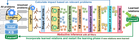
Figure 4: Learning starts with an initial KB. Abduction is carried out on unsolved entailment and contradiction problems. Inferred knowledge, i.e., T-sets, pass several filters to select the best knowledge. The learned knowledge is added to the initial KB, and the learning phase repeats until no new knowledge is learned.

Following (A1), a relation has to be semantically consistent with existing KB. In this way, relations like $\textbf{{hedgehog}}\,|\,{}\textbf{{animal}}$ or $\textbf{{big}}\!\sqsubseteq\!{}\textbf{{small}}$ will be dubbed inconsistent with KB which includes $\textbf{{hedgehog}}\!\sqsubseteq\!{}\textbf{{animal}}$ and $\textbf{{big}}\,|\,{}\textbf{{small}}$. In experiments, instead of doing a complete consistency checking of the entire KB every time a new relation is considered, we perform a lazy check by verifying whether $A\,|\,{}B$ and one of $A\!\sqsubseteq\!{}B$ and $B\!\sqsubseteq\!{}A$ together occur in KB. We go further and ignore relations of form $B\,|\,{}AB$ taking into account that subsective lexical modifiers are prevalent. Hence, relations like $\textbf{{small animal}}\,|\,{}\textbf{{animal}}$ will be dropped.

Additionally, we consider only such T-sets that are semantically consistent with sentences of the corresponding NLI problem. This can be seen as further elaboration on (A2) since the sentences are usually consistent with background knowledge. The example of a bad T-set, inconsistent with the sentence, is the one containing $\textbf{{baby}}\,|\,{}\textbf{{panda}}$ when one of the sentences of the NLI problem asserts the existence of a baby panda: Two baby pandas are playing (sk-5435). Both filters concerning semantic consistency with KB or sentences are used to weed out pseudo-knowledge.

Another adopted criterion for the best T-sets is an impact on accuracy on the training data, which is calculated as a difference between the number of solved and unsolved problems in the training data when a T-set is adopted. T-sets with no positive impact on accuracy will be ignored as it doesn’t contribute to the performance. This criterion can be broadly related to (A1), where a T-set is supposed to conform to the gold labels. For example, if a T-set $\{\textbf{{boy}}\!\sqsubseteq\!{}\textbf{{young}},\textbf{{hedgehog}}\!\sqsubseteq\!{}\textbf{{small}}\}$ helps to solve two new problems but unsolves at least two previously solved ones, then it won’t be learned. For the same NLI problem, a T-set with the highest impact will be preferred over others. The motivation behind this criterion is to favor the relations that boost accuracy on the training data.

Despite introduced filters and comparison orders for T-sets, some problems can still have more than one best T-sets. In such cases, we take into account the number of terms in T-sets (by counting occurrences of atomic terms). At the end we opt for the T-set with the smallest number of terms. This decision somewhat complies with (A2).

4 Experiments

We design experiments to evaluate learning as abduction for NLI. First, we implement the abductive learning for LangPro Abzianidze (2017a). The implementation takes advantage of Prolog’s virtue of satisfying goals in the forward and backward fashion and uses it to apply closure rules in backwards during the search for B-sets. This leaves the inventory of tableau rules intact. The workflow of the abductive learning is depicted in Figure 4.

Searching for the best T-set is an NP-hard problem. To make the implementation efficient (q1), we significantly reduce a space of T-sets by considering only those T-sets that coincide with B-sets. In other words, we require existence of the shared B-sets across all open branches. The example in Subsection 3.1 doesn’t have such T-set as different B-sets close the open branches. If a tableau has a single open branch, its B-sets are automatically T-sets.

To test the learning algorithm, we use the sick dataset Marelli et al. (2014b) for three reasons. First, compositional lexical knowledge involved in the dataset is suitable for the abductive learning. Second, it is large enough (up to 10K problems) to support learning from a training part and evaluation on an unseen part. Third, sick has been used for evaluating logic-based NLI systems, including LangPro, and this allows comparison to the existing results. Our data partition follows the SemEval-14 task-1 Marelli et al. (2014a): sick-train&trial (4500 + 500 problems) is a training data and sick-test (4927 problems) a hidden test data. The error analysis is conducted only on the training data. To choose optimal learning parameters (see Subsection 3.3) and measure impact of the filters and knowledge resources, we run the learning algorithm with stratified three-fold cross-validation (CV) on the training data. The stratified version is due to a skewed distribution of gold labels in sick. We opt for three-fold CV as it better reflects 1:1 ratio between sick-train&trial and -test sizes.

Logic-based NLI systems using logical forms from syntactic trees often employ output of several parsers to increase the quality of logical forms Abzianidze (2015); Beltagy et al. (2016); Martínez-Gómez et al. (2017); Yanaka et al. (2018). In our CV experiments, we use the re-banked C&C CCG parser Clark and Curran (2007); Honnibal et al. (2010). The ensemble of parsers, used for evaluation on sick-test, additionally includes EasyCCG Lewis and Steedman (2014) and DepCCG Yoshikawa et al. (2017) with standard models.

5 Results

Initially we run LangPro with WordNet Miller (1995) relations and all filters enabled (see Subsection 3.3). The results in Table 1 lead to several findings. The abductive learning does help to improve accuracy. LangPro without abduction (with 800 rule applications) gets 81.7% accuracy on sick-train&test while with abduction it obtains 82.9% on average over unseen parts of CV on sick-train&test. Differences between average accuracies on training and test parts show that overfitting during training is moderate. When the prover is limited to 50 rule app., accuracy drops only to 82.64%. However, the entire CV takes almost 10 times less CPU time for 50 rule app. compared to 800. These results answer (q1) by rendering the abductive learning as a computationally feasible learning method.

We conduct ablation experiments to verify the contributions of the filters. Table 1 shows that filters concerning semantic consistency and syntactic comparability together have little impact on accuracy (.32%), but they contribute to efficiency by halving CPU time. This means that other filters like impact on accuracy and term size greatly contribute to preventing pseudo-knowledge. When relations in T-sets are restricted to atomic terms (i.e., terms of length 1), accuracy is almost unchanged (-0.16%) while efficiency slightly increases. The increase in efficiency is clear as fewer T-sets will be considered during learning. Little change in accuracy means that mostly relations over atomic terms generalize well over the unseen part.

We also tested whether the learned relations can compensate for the WordNet relations (q3). The results show that WordNet relations still contribute to high accuracy as their exclusion drops accuracy by 2.44%. Abzianidze (2015) uses hand-crafted KB of $\sim$30 lexical relations collected from sick-train&trial. When this KB is add, only six more problems on average (0.36%) is classified correctly.

To answer (q4), we compare LangPro with and without abduction on unseen sick-test. The results in Table 3 show that the abductive learning consistently increases accuracy regardless of the used CCG parser. This also means that the abductive learning generalizes across CCG parsers. When predictions of three LangPro versions with C&C, EasyCCG and DepCCG parsers are aggregated, accuracy gain from abduction still remains (+1.36%, additional 67 problems solved). It is worth noting that while abduction increases the overall accuracy, almost perfect precision (>97.6%) of LangPro decreases only to 94.3%. We argue that this is an important virtue of the abductive learning from a logic perspective since logic-based NLI systems are expected to have highly reliable proofs.

LangPro + Abductive learning: All filters + WordNet	Train av. acc%	Test av. acc%	CPU time
max 800 rule applications	89.02	82.90	2041
max 50 rule applications	88.57	82.64	220
Ablation with max 50 rule app.	$\Delta$	$\Delta$	$\Delta$
$-$ CT, CwS, CwKB	+1.39	-0.32	+115%
$-$ terms of length 2 & 3	-2.68	-0.16	-17%
$-$ WN rels: ant,hyp,der,sim	-0.98	-2.44	-11%
$+$ Hand-crafted ✍ KB	+0.04	+0.36	+1%

Table 1: Results of the CV on sick-train&trial (majority baseline = 56.4%). Ablation experiments disable filters for comparable terms (CT) and consistencies with sentences (CwS) and KB (CwKB). CPU time (for 2.5 GHz) is measured in minutes for the entire CV.

6 Error Analysis

In total 312 relations were learned with abduction from sick-train&trial based on a single parser. Table 2 lists some of the learned relations. We classify relations into four groups based on whether they are mostly correct, wrong, reversed version of a correct relation, and highly context-dependent.

Despite having a sequence of filters, substantial pseudo-knowledge (29%) still leaked during the learning. One of the main reasons for this is a strong learning bias towards minimal explanations which often leads to ignoring context. This way, from sk-9624 …is looking toward the stars… entailing …is looking toward the sky…, $\textbf{{star}}\!\sqsubseteq\!{}\textbf{{sky}}$ relation was wrongly learned. Additionally, learning $\textbf{{in the dark}}\!\sqsubseteq\!{}\textbf{{at night}}$ is preferred to currently learned $\textbf{{in}}\!\sqsubseteq\!{}\textbf{{at}}$. This is a common drawback of pure logic-based approaches which is induced by a general principle, called a rule of replacement, which licenses replacement of equivalent terms.

A number of incorrect learned relations are conditioned by noisy gold labels of sick Kalouli et al. (2017). $\textbf{{dog}}\!\sqsubseteq\!{}\textbf{{bull dog}}$ was learned due to sk-2608, A monkey is brushing the dog contradicting The monkey is not brushing a bull dog; $\textbf{{person}}\!\sqsubseteq\!{}\textbf{{man}}$ is due to sk-4680, Someone is drilling a hole in a strip of wood with a power drill entailing A man is drilling a hole in a piece of wood.

Correct (26.6%)	Wrong (28.8%)
add X to Y$\,|\,{}\textbf{{remove}}$ X from Y	the blonde girl$\,|\,{}$a little girl
a X $\textbf{{lie down}}\,|\,{}$a X run around	aim a gun $\!\sqsubseteq\!{}\,\textbf{{draw}}$ a gun
perform $\textbf{{acrobatics}}\!\sqsubseteq\!{}$perform a trick	ride in X$\,|\,{}\textbf{{get}}$ out of X
Reversed (28.9%)	Contextual (15.7%)
have lunch $\!\sqsubseteq\!{}\textbf{{eat}}$	hang on a $\textbf{{cord}}\!\sqsubseteq\!{}$hang on a rope
look at X $\!\sqsubseteq\!{}\textbf{{stare}}$ at X	man in a $\textbf{{cap}}\!\sqsubseteq\!{}$man in a hat
prepare some $\textbf{{food}}\!\sqsubseteq\!{}$prepare a meal	in the dark $\!\sqsubseteq\!{}\,\textbf{{at}}$ night

Table 2: Examples of learned lexical relations. The terms of the relations are in boldface while padded gray contexts come from the source sick problems. The relations are manually assessed by the author outside context of sick problems.

7 Related Work & Comparison

The closest work to ours, to the best of our knowledge, represents Yanaka et al. (2018). They use abduction for a logic-based NLI system to automatically acquire phrase correspondences from labeled NLI problems. Their method, called P2P, converts logical formulas into graphs and carries out subgraph matching with variable unification. Our work differs from theirs in four aspects: (i) employed formal logics and proof procedures essentially differ from each other. (ii) Converting formulas into graphs and matching subgraphs is external to their theorem proving while in our approach the abductive learning is the theorem proving run backwards. (iii) P2P abstracts from term comparability constraint and learns relations across word classes. It also reduces lexical relations to smaller axioms. In total P2P extracts 9445 axioms from sick-train&trial compared to 312 relations by our abductive learning. (iv) P2P scarifies a substantial amount of precision (12.9%) to gain 1.2% of accuracy while our abductive learning achieves more gain in accuracy with much less drop in precision.

System	Parsers	Learn	MLc	KB&Res.	P%	R%	A%
➥LangPro	C	$-$	$-$	WN	97.8	58.0	81.3
➥LangPro	C	Abd	$-$	WN	94.9	63.4	82.7
➥LangPro	E	$-$	$-$	WN	97.7	57.7	81.1
➥LangPro	E	Abd	$-$	WN	94.9	63.0	82.5
➥LangPro	D	$-$	$-$	WN	97.8	59.2	81.8
➥LangPro	D	Abd	$-$	WN	94.8	64.3	83.0
➥LangPro	CDE	$-$	$-$	WN	97.6	62.2	83.0
➥LangPro	CDE	Abd	$-$	WN	94.3	67.9	84.4
LangPro 2015	DCE	$-$	$-$	WN,✍KB	98.0	58.1	81.4
MG et al. 2017	DCE	W2W	$-$	WN,VO	97.1	63.6	83.1
Yanaka et al.	CDE	W2W,P2P	$-$	WN,VO	84.2	77.3	84.3
★Bjerva et al.	C	$-$	SVM	WN,PP	93.6	60.6	81.6
Pavlick et al.	C	$-$	$-$	WN,PP+			78.4
★Beltagy et al.	C	$-$	SVM	WN	97.9	38.7	73.2
Beltagy and Erk	C	$-$	SVM	WN			76.5
Beltagy et al.	CE	Rob.Res.	SVM	WN,PP,Dist,✍Rules			85.1
Hu et al. (2020)	CE	$-$	$-$	WN	83.8	70.7	77.2
$+$ BERT Devlin et al. (2019)							85.4
★Lai and Hockenmaier (winner of the SemEval task)							84.6
Yin and Schütze DL with GRU & Attentive Pooling							87.1

Table 3: Comparison of LangPro₈₀₀+Abduction and other logic-based systems on sick-test. Some results are not directly comparable as the systems use different KB, resources, CCG parsers, or even employ a machine learning classifier (MLc). Systems are grouped based on their characteristic approaches to NLI. The last two systems are not based on logic. A list of abbreviations: current work (➥), SemEval-14 task-1 participants (★), C&C parser (C), EasyCCG (E), DepCCG (D), PPDB (PP, Ganitkevitch et al., 2013), and VerbOcean (VO, Chklovski and Pantel, 2004).

There have been several logic-based NLI systems evaluated on sick. We believe Table 3 lists all (but not only) of those systems along with their scores. The research line by Mineshima et al. (2015); Martínez-Gómez et al. (2017); Yanaka et al. (2018) was already described while comparing their approach to ours. The work by Bjerva et al. (2014); Pavlick et al. (2015) employ Boxer Bos (2008) to obtain first-order logic formulas from sentences and use an SVM classifier on top of Nutcracker Bos and Markert (2005), which reasons using off-the-shelf theorem prover and model builder. Beltagy et al. (2014, 2016) also uses Boxer to get first-order logic formulas but employs probabilistic logic inference in Markov Logic Networks. To hit the high score on sick, they combine multiple components including distributional semantics, a set of hand-crafted rules, resolution-based on-fly generation of inference rules, and an SVM classifier as the final predictor. Hu et al. (2019) use a lightweight system, called MonaLog, based on monotonicity reasoning. It is further combined with BERT Devlin et al. (2019) to reclassify problems that were predicted by MonaLog as neutral.

Abductive reasoning was already employed by Raina et al. (2005) at the first Recognizing Textual Entailment challenge Dagan et al. (2005). They used resolution method and a learned cost model to select the cheapest set of assumptions supporting the entailment. Hobbs et al. (1993) uses weighted abduction to model text interpretation as the minimal explanation of why text would be true. The title of the current paper is inspired by this work.

8 Conclusion

Table 3 shows that the abductive learning component is crucial for logic-based reasoning systems to achieve competitive results. We have implemented and showed that learning as abduction works successfully for tableau theorem prover the theorem prover to learn lexical relations from data. Our findings answer the predefined research question as follows. (q1) Implementing abduction as backwards theorem proving represents a computationally feasible approach for data-driven learning. This was achieved by reducing the explanation space: considering only those T-sets that are shared by all open branches and applying several filters to them. (q2) Pseudo-knowledge is partially prevented with a sequence of filters and comparison criteria. Abductive bias towards minimality often leads to relations that require additional context. Overall, pseudo-knowledge doesn’t harm high precision of the theorem proving. (q3) Despite knowledge learned from data, the lexical relations extracted from WordNet are crucial to reach the state-of-the-art results. (q4) Abductive learning consistently increases the accuracy score of the prover regardless of using different parsers individually or in ensemble.

For future work it is interesting to explore the ways that consider larger explanation space and are not strictly preferring short phrases to longer ones. The latter will allow relations with more context.

Acknowledgments

I would like to thank three anonymous reviewers for their valuable comments and the CIT of the University of Groningen for providing access to the Peregrine HPC cluster. This work was supported by the NWO-VICI grant (288-89-003) while I was at the University of Groningen and by the European Research Council (ERC) under the European Unions Horizon 2020 research and innovation programme (grant agreement No. 742204) since I joined Utrecht University.

References

• Abzianidze (2015) Lasha Abzianidze. 2015. A tableau prover for natural logic and language. In Proceedings of the 2015 Conference on Empirical Methods in Natural Language Processing, pages 2492–2502, Lisbon, Portugal. Association for Computational Linguistics.
• Abzianidze (2017a) Lasha Abzianidze. 2017a. LangPro: Natural language theorem prover. In Proceedings of the 2017 Conference on Empirical Methods in Natural Language Processing: System Demonstrations, pages 115–120, Copenhagen, Denmark. Association for Computational Linguistics.
• Abzianidze (2017b) Lasha Abzianidze. 2017b. A natural proof system for natural language. Ph.D. thesis, Tilburg University.
• Beltagy et al. (2016) I. Beltagy, Stephen Roller, Pengxiang Cheng, Katrin Erk, and Raymond J. Mooney. 2016. Representing meaning with a combination of logical and distributional models. Computational Linguistics, 42(4):763–808.
• Beltagy and Erk (2015) Islam Beltagy and Katrin Erk. 2015. On the proper treatment of quantifiers in probabilistic logic semantics. In Proceedings of the 11th International Conference on Computational Semantics, pages 140–150, London, UK. Association for Computational Linguistics.
• Beltagy et al. (2014) Islam Beltagy, Stephen Roller, Gemma Boleda, Katrin Erk, and Raymond Mooney. 2014. UTexas: Natural language semantics using distributional semantics and probabilistic logic. In Proceedings of the 8th International Workshop on Semantic Evaluation (SemEval 2014), pages 796–801, Dublin, Ireland. Association for Computational Linguistics.
• van Benthem (2008) Johan van Benthem. 2008. A brief history of natural logic. In Technical Report PP-2008-05. Institute for Logic, Language & Computation.
• Bjerva et al. (2014) Johannes Bjerva, Johan Bos, Rob van der Goot, and Malvina Nissim. 2014. The meaning factory: Formal semantics for recognizing textual entailment and determining semantic similarity. In Proceedings of the 8th International Workshop on Semantic Evaluation (SemEval 2014), pages 642–646, Dublin, Ireland. Association for Computational Linguistics.
• Bos (2008) Johan Bos. 2008. Wide-coverage semantic analysis with boxer. In Semantics in Text Processing. STEP 2008 Conference Proceedings, Research in Computational Semantics, pages 277–286. College Publications.
• Bos and Markert (2005) Johan Bos and Katja Markert. 2005. Recognising textual entailment with logical inference. In Proceedings of the 2005 Conference on Empirical Methods in Natural Language Processing (EMNLP 2005), pages 628–635.
• Chklovski and Pantel (2004) Timothy Chklovski and Patrick Pantel. 2004. VerbOcean: Mining the web for fine-grained semantic verb relations. In Proceedings of the 2004 Conference on Empirical Methods in Natural Language Processing, pages 33–40, Barcelona, Spain. Association for Computational Linguistics.
• Clark and Curran (2007) Stephen Clark and James R. Curran. 2007. Wide-coverage efficient statistical parsing with CCG and log-linear models. Computational Linguistics, 33(4):493–552.
• Cooper et al. (1996) Robin Cooper, Dick Crouch, Jan Van Eijck, Chris Fox, Josef Van Genabith, Jan Jaspars, Hans Kamp, David Milward, Manfred Pinkal, Massimo Poesio, Steve Pulman, Ted Briscoe, Holger Maier, and Karsten Konrad. 1996. FraCaS: A Framework for Computational Semantics. Deliverable D16.
• Dagan et al. (2005) Ido Dagan, Oren Glickman, and Bernardo Magnini. 2005. The pascal recognising textual entailment challenge. In Proceedings of the PASCAL Challenges Workshop on Recognising Textual Entailment.
• Dagan et al. (2013) Ido Dagan, Dan Roth, Mark Sammons, and Fabio Massimo Zanzotto. 2013. Recognizing Textual Entailment: Models and Applications. Synthesis Lectures on Human Language Technologies. Morgan & Claypool Publishers.
• Devlin et al. (2019) Jacob Devlin, Ming-Wei Chang, Kenton Lee, and Kristina Toutanova. 2019. BERT: Pre-training of deep bidirectional transformers for language understanding. In Proceedings of the 2019 Conference of the North American Chapter of the Association for Computational Linguistics: Human Language Technologies, Volume 1 (Long and Short Papers), pages 4171–4186, Minneapolis, Minnesota. Association for Computational Linguistics.
• Ganitkevitch et al. (2013) Juri Ganitkevitch, Benjamin Van Durme, and Chris Callison-Burch. 2013. PPDB: The paraphrase database. In Proceedings of NAACL-HLT, pages 758–764, Atlanta, Georgia. Association for Computational Linguistics.
• Glockner et al. (2018) Max Glockner, Vered Shwartz, and Yoav Goldberg. 2018. Breaking NLI systems with sentences that require simple lexical inferences. In Proceedings of the 56th Annual Meeting of the Association for Computational Linguistics (Volume 2: Short Papers), pages 650–655, Melbourne, Australia. Association for Computational Linguistics.
• Gururangan et al. (2018) Suchin Gururangan, Swabha Swayamdipta, Omer Levy, Roy Schwartz, Samuel Bowman, and Noah A. Smith. 2018. Annotation artifacts in natural language inference data. In Proceedings of the 2018 Conference of the North American Chapter of the Association for Computational Linguistics: Human Language Technologies, Volume 2 (Short Papers), pages 107–112, New Orleans, Louisiana. Association for Computational Linguistics.
• Hobbs et al. (1993) Jerry R. Hobbs, Mark Stickel, and Paul Martin. 1993. Interpretation as abduction. Artificial Intelligence, 63:69–142.
• Honnibal et al. (2010) Matthew Honnibal, James R. Curran, and Johan Bos. 2010. Rebanking CCGbank for improved NP interpretation. In Proceedings of the 48th Annual Meeting of the Association for Computational Linguistics, pages 207–215, Uppsala, Sweden. Association for Computational Linguistics.
• Hu et al. (2019) Hai Hu, Qi Chen, and Larry Moss. 2019. Natural language inference with monotonicity. In Proceedings of the 13th International Conference on Computational Semantics - Short Papers, pages 8–15, Gothenburg, Sweden. Association for Computational Linguistics.
• Hu et al. (2020) Hai Hu, Qi Chen, Kyle Richardson, Atreyee Mukherjee, Lawrence S Moss, and Sandra Kübler. 2020. Monalog: a lightweight system for natural language inference based on monotonicity. Proceedings of the Society for Computation in Linguistics, 3(1):319–329.
• Kalouli et al. (2017) Aikaterini-Lida Kalouli, Valeria de Paiva, and Livy Real. 2017. Correcting contradictions. In Proceedings of the Computing Natural Language Inference Workshop.
• Lai and Hockenmaier (2014) Alice Lai and Julia Hockenmaier. 2014. Illinois-LH: A denotational and distributional approach to semantics. In Proceedings of the 8th International Workshop on Semantic Evaluation (SemEval 2014), pages 329–334, Dublin, Ireland. Association for Computational Linguistics.
• Lewis and Steedman (2014) Mike Lewis and Mark Steedman. 2014. A* CCG parsing with a supertag-factored model. In Proceedings of the 2014 Conference on Empirical Methods in Natural Language Processing (EMNLP), pages 990–1000, Doha, Qatar. Association for Computational Linguistics.
• Marelli et al. (2014a) Marco Marelli, Luisa Bentivogli, Marco Baroni, Raffaella Bernardi, Stefano Menini, and Roberto Zamparelli. 2014a. SemEval-2014 task 1: Evaluation of compositional distributional semantic models on full sentences through semantic relatedness and textual entailment. In Proceedings of the 8th International Workshop on Semantic Evaluation (SemEval 2014), pages 1–8, Dublin, Ireland. Association for Computational Linguistics.
• Marelli et al. (2014b) Marco Marelli, Stefano Menini, Marco Baroni, Luisa Bentivogli, Raffaella Bernardi, and Roberto Zamparelli. 2014b. A SICK cure for the evaluation of compositional distributional semantic models. In Proceedings of the Ninth International Conference on Language Resources and Evaluation (LREC-2014), pages 216–223, Reykjavik, Iceland. European Languages Resources Association (ELRA).
• Martínez-Gómez et al. (2017) Pascual Martínez-Gómez, Koji Mineshima, Yusuke Miyao, and Daisuke Bekki. 2017. On-demand injection of lexical knowledge for recognising textual entailment. In Proceedings of the 15th Conference of the European Chapter of the Association for Computational Linguistics: Volume 1, Long Papers, pages 710–720, Valencia, Spain. Association for Computational Linguistics.
• Mayer and Pirri (1993) Marta Cialdea Mayer and Fiora Pirri. 1993. First order abduction via tableau and sequent calculi. Logic Journal of the IGPL, 1(1):99–117.
• Miller (1995) George A. Miller. 1995. Wordnet: A lexical database for english. Communications of the ACM, 38(11):39–41.
• Mineshima et al. (2015) Koji Mineshima, Pascual Martínez-Gómez, Yusuke Miyao, and Daisuke Bekki. 2015. Higher-order logical inference with compositional semantics. In Proceedings of the 2015 Conference on Empirical Methods in Natural Language Processing, pages 2055–2061, Lisbon, Portugal. Association for Computational Linguistics.
• Moss (2010) Lawrence S. Moss. 2010. Natural logic and semantics. In Maria Aloni, Harald Bastiaanse, Tikitu de Jager, and Katrin Schulz, editors, Logic, Language and Meaning: 17th Amsterdam Colloquium, Amsterdam, The Netherlands, December 16-18, 2009, Revised Selected Papers, pages 84–93. Springer Berlin Heidelberg, Berlin, Heidelberg.
• Muskens (2010) Reinhard Muskens. 2010. An analytic tableau system for natural logic. In Maria Aloni, Harald Bastiaanse, Tikitu de Jager, and Katrin Schulz, editors, Logic, Language and Meaning, volume 6042 of Lecture Notes in Computer Science, pages 104–113. Springer Berlin Heidelberg.
• Pavlick et al. (2015) Ellie Pavlick, Johan Bos, Malvina Nissim, Charley Beller, Benjamin Van Durme, and Chris Callison-Burch. 2015. Adding semantics to data-driven paraphrasing. In Proceedings of the 53rd Annual Meeting of the Association for Computational Linguistics and the 7th International Joint Conference on Natural Language Processing (Volume 1: Long Papers), pages 1512–1522, Beijing, China. Association for Computational Linguistics.
• Poliak et al. (2018) Adam Poliak, Jason Naradowsky, Aparajita Haldar, Rachel Rudinger, and Benjamin Van Durme. 2018. Hypothesis only baselines in natural language inference. In Proceedings of the Seventh Joint Conference on Lexical and Computational Semantics, pages 180–191, New Orleans, Louisiana. Association for Computational Linguistics.
• Raina et al. (2005) Rajat Raina, Andrew Y. Ng, and Christopher D. Manning. 2005. Robust textual inference via learning and abductive reasoning. In Proceedings of AAAI 2005. AAAI Press.
• Steedman (2000) Mark Steedman. 2000. The Syntactic Process. MIT Press, Cambridge, MA, USA.
• Yanaka et al. (2018) Hitomi Yanaka, Koji Mineshima, Pascual Martínez-Gómez, and Daisuke Bekki. 2018. Acquisition of phrase correspondences using natural deduction proofs. In Proceedings of the 2018 Conference of the North American Chapter of the Association for Computational Linguistics: Human Language Technologies, Volume 1 (Long Papers), pages 756–766, New Orleans, Louisiana. Association for Computational Linguistics.
• Yin and Schütze (2017) Wenpeng Yin and Hinrich Schütze. 2017. Task-specific attentive pooling of phrase alignments contributes to sentence matching. In Proceedings of the 15th Conference of the European Chapter of the Association for Computational Linguistics: Volume 1, Long Papers, pages 699–709, Valencia, Spain. Association for Computational Linguistics.
• Yoshikawa et al. (2017) Masashi Yoshikawa, Hiroshi Noji, and Yuji Matsumoto. 2017. A* CCG parsing with a supertag and dependency factored model. In Proceedings of the 55th Annual Meeting of the Association for Computational Linguistics (Volume 1: Long Papers), pages 277–287, Vancouver, Canada. Association for Computational Linguistics.