Quantum scattering process and information transfer
out of a black hole

Abstract

We calculate the probability amplitude for tree-level elastic electron-muon scattering in Minkowski spacetime with carefully prepared initial and final wave packets. The obtained nonzero amplitude implies a nonvanishing probability for detecting a recoil electron outside the light-cone of the initial muon. Transposing this Minkowski-spacetime scattering result to a near-horizon spacetime region of a massive Schwarzschild black hole and referring to a previously proposed Gedankenexperiment, we conclude that, in principle, it is possible to have information transfer from inside the black-hole horizon to outside.

Acta Phys. Pol. B 52, 805 (2021) arXiv:2010.15787

04.20.Cv, 04.70.-s, 12.20.-m

1 Introduction

It is often said that nothing can come out of a black hole (cf. Sec. 33.1 of Ref. [1]). This statement may, however, be not quite correct, as we have argued previously [2] that information can come out. The information is carried not by a particle but by momentum transfer in a quantum scattering process. In fact, the information-transfer process is based not on a faster-than-light signal exchange but on a virtual photon exchange. This leads to dynamical entanglement between two initially unentangled charged particles which are located at different sides of the black-hole horizon. A Gedankenexperiment [2] relying on such momentum transfer (or its absence, i.e., no quantum scattering) allows, in principle, for the transmittal of an elementary message (bit value “1” or “0”) from inside the black-hole horizon to outside the black-hole horizon.

The goal of the present paper is to present a straightforward quantum-electrodynamics [3, 4] calculation that indisputably shows the nonvanishing probability for having such a momentum transfer. Specifically, we consider a carefully prepared $2$–$2$ scattering process in Minkowski spacetime. According to the Einstein Equivalence Principle, this Minkowski-spacetime scattering process is relevant for the near-horizon spacetime region of a large-enough black hole; see Fig. 1 for a sketch. This near-horizon region with local inertial coordinates is described by a patch of Minkowski spacetime with a projected black-hole horizon that corresponds to part of a light-cone (see Fig. 2 in Ref. [2]).

The setup of our $2$–$2$ scattering process in Minkowski spacetime involves a muon $\mu^{-}$ and an electron $e^{-}$, where the initial muon is strictly localized inside the projected black-hole horizon and the initial electron, localized with large probability outside the projected black-hole horizon, has strictly an incoming 3-momentum (i.e., 3-momentum directed towards the black hole center). The aim of the calculation is to establish a nonzero probability for finding, at a later time, an outgoing electron (3-momentum directed away from the black hole center) by use of a large detector positioned outside the projected black-hole horizon.

Let us immediately put to rest possible worries about causality. The setup of the Minkowski-spacetime scattering process is such that there is an extended initial state and the final recoil electron lies within the outermost light cone of the initial electron, so that there is no problem with causality. As mentioned above, the final electron-muon state is entangled, whereas the initial electron-muon state is not [2].

The outline of our paper is as follows. In Sec. 2, we describe carefully chosen wave packets in Minkowski spacetime for the initial and final muons and electrons. In Sec. 3, we calculate the scattering probability amplitude of these initial and final particles in quantum electrodynamics and obtain a nonzero probability amplitude for detecting a recoil electron outside the light-cone of the initial muon. (The scattering-probability-amplitude calculation of the present paper improves upon the one of App. C in Ref. [2] precisely by the detailed discussion of appropriate initial and final wave packets.) In Sec. 4, we transpose the Minkowski-spacetime result to a near-horizon spacetime region of a massive Schwarzschild black hole and recall the essential steps of a Gedankenexperiment from our previous paper [2], which then allows for information transfer from inside the black-hole horizon to outside.

It is possible, in a first reading, to skip the technical details and to move immediately to Secs. 3.3 and 4.

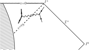
Figure 1: Sketch of an elastic electron-muon scattering process in the near-horizon region of a massive Schwarzschild black hole. Shown is part of the Penrose conformal diagram of the Schwarzschild black hole in Kruskal–Szekeres coordinates (see Figs. 34.3 and 32.1.b of Ref. [1] for details). The Schwarzschild horizon $r=r_{S}\equiv 2GM_{\text{BH}}/c^{2}$ is indicated by the dashed line and the matter of a spherically-symmetric collapsing star by the shaded region on the left of the figure. The scattering process is shown symbolically by a position-space Feynman diagram [3] with a single line for the electron, a double line for the muon, and a wavy line for the exchange photon.

2 Free wave packets in Minkowski spacetime

2.1 General wave-packet solution

We consider a general wave-packet solution of the free Dirac equation for mass $M$, with center-of-mass parameters $X^{a}=(X^{0},\mathbf{X})$ in position space and $P^{a}=(P^{0},\mathbf{P})$ in momentum space (the localization regions satisfy the Heisenberg uncertainty relations). With gamma matrices in the Weyl representation, this solution reads

$$\psi_{X,P}(x) \equiv {\int}\frac{d^{4}Q}{(2\pi)^{3}}\,\theta\big{(}Q^{0}\big{)}\,\delta\big{(}Q^{2}-M^{2}\big{)}F_{P}(Q)\,u(Q)\,e^{-iQ{\cdot}(x-X)}\,,$$ (1a)

where spinor indices have been suppressed and

$$u(Q) = \left(\begin{array}[]{c}\sqrt{Q{\cdot}\sigma}\,\xi\\[2.84526pt] \sqrt{Q{\cdot}\bar{\sigma}}\,\xi\\ \end{array}\right),$$ (1d)

with a two-component spinor $\xi$ normalized by $\xi^{\dagger}\xi=1$. We shall assume in what follows that $\xi^{T}=(1,\,0)$. Furthermore, $\sigma^{a}\equiv\big{(}\sigma^{0},\,+\sigma^{i}\big{)}$ and $\bar{\sigma}^{a}\equiv\big{(}\sigma^{0},\,-\sigma^{i}\big{)}$ are two matrix-valued four-vectors with $\sigma^{0}$ and $\sigma^{i}$ standing for the $2{\times}2$ identity matrix and the three Pauli matrices.

With a momentum wave function $F_{P}(Q)$ peaking at $Q=P$, the normalized quantum state $|\psi_{X,P}\rangle$ associated with the position wave function $\psi_{X,P}(x)$ from (1) has

$$\langle\psi_{X,P}|\psi_{X,P}\rangle \equiv \int_{\mathbb{R}^{3}}d^{3}\mathbf{x}\,\big{(}\psi_{X,P}(x)\big{)}^{\dagger}\,\psi_{X,P}(x)$$ (2)

$$= \frac{1}{2}{\int}\frac{d^{3}\mathbf{Q}}{(2\pi)^{3}}\,\frac{|F_{P}(\mathbf{Q})|^{2}}{\sqrt{|\mathbf{Q}|^{2}+M^{2}}}\;=\;1\,.$$

Throughout this paper, we use natural units with $c=1$ and $\hbar=1$. For standard Cartesian coordinates,

$$x^{a} = \Big{[}\big{(}x^{0},\,\mathbf{x}\big{)}\Big{]}^{a}=\Big{[}\big{(}x^{0},\,x^{1},\,x^{2},\,x^{3}\big{)}\Big{]}^{a}\,,$$ (3a)

the Minkowski metric reads

$$\eta_{ab} = \Big{[}\text{diag}\big{(}1,\,-1,\,-1,\,-1\big{)}\Big{]}_{ab}\,,$$ (3b)

where the spacetime indices $a,\,b$ run over $\{0,\,1,\,2,\,3\}$. Occasionally, we will write

$$x^{0}=c\,t=t\,.$$ (4)

2.2 Muon wave packets

2.2.1 Muon-wave-packet Ansatz

We take the following Ansatz for the momentum wave function of the muon ($\mu$):

$$\big{(}F_{P}(Q)\big{)}_{\mu} = N_{\mu}\,2\,Q^{0}\,\prod_{i=1}^{i=3}\,\text{sinc}\left(\frac{Q_{i}-P_{i}}{D}\right)\,,$$ (5)

where $N_{\mu}$ is the normalization factor, $D$ the momentum variance, and ‘sinc’ the standard function

$$\text{sinc}(x)\equiv\frac{\sin\,x}{x}\,,$$ (6)

for $x\in\mathbb{R}$.

In order to guarantee that the undisturbed wave packet essentially propagates as a free classical particle, we assume that the particle Compton wavelength is much smaller than the packet localization size (see below). Taking $M_{\mu}\gg D$ in (5), we obtain for the muon wave packet from (1)

$$\big{(}\psi_{X,P}(x)\big{)}_{\mu} \approx \mu_{X,P}(x)$$ (7)

$$\equiv \frac{N_{\mu}}{(2/D)^{3}}\,u(P)\,e^{-iP{\cdot}\Delta{x}}\prod_{i=1}^{i=3}\,\text{rect}\left(\frac{P^{i}\Delta{x}^{0}-P^{0}\Delta{x}^{i}}{2P^{0}/D}\right),$$

where

$$\Delta{x}^{\mu} \equiv x^{\mu}-X^{\mu}\,,$$ (8)

and where the top-hat function ‘$\text{rect}(x)$’, for $x\in\mathbb{R}$, is defined as follows:

$$\text{rect}(x) \equiv \left\{\begin{array}[]{lcll}1\,,&|x|&<&1/2\,,\\[2.84526pt] 1/2\,,&|x|&=&1/2\,,\\[2.84526pt] 0\,,&|x|&>&1/2\,.\end{array}\right.$$ (12)

The right-hand side of (7) has nonvanishing support over a finite spatial region,

$$\Delta{x}^{i} \in \left[P^{i}\Delta{x}^{0}/P^{0}-1/D,\,P^{i}\Delta{x}^{0}/P^{0}+1/D\right]\,,$$ (13)

which will be an important input for the setup to be discussed in the rest of this section.

2.2.2 Muon-wave-packet normalization and boundary conditions

The normalization factor $N_{\mu}$ can now be directly computed with $\mu_{X,P}(x)$ from (7). Specifically, we find that

$$N_{\mu,\,\text{approx.}}=\sqrt{\frac{4}{P_{0}\,D^{3}}}\;\Rightarrow\;N_{\mu,\,i,\,\text{approx.}}=N_{\mu,\,f,\,\text{approx.}}\approx\frac{0.036965}{D^{2}}\,,$$ (14)

where we assume that

$$M_{\mu} = 2070\,D$$ (15)

and that the initial ($i$) and final ($f$) conditions for the muon wave packets are, respectively,

$$(X)_{\mu,\,i}\,D \approx \big{(}0.00,\,-3.54,\,0.00,\,0.00\big{)}\,,$$ (16a)

$$(P)_{\mu,\,i}\big{/}D \approx \big{(}2927.42,\,2070.00,\,0.00,\,0.00\big{)}\,,$$ (16b)

and

$$(X)_{\mu,\,f}\,D \approx \big{(}10.00,\,-2.04,\,2.89,\,0.00\big{)}\,,$$ (16c)

$$(P)_{\mu,\,f}\big{/}D \approx \big{(}2927.42,\,-1195.12,\,1690.15,\,0.00\big{)}\,.$$ (16d)

The specific numerical values for $(X)_{\mu,\,i}$ and $(X)_{\mu,\,f}$ have been chosen, so that the position of the undisturbed initial and final muon wave packets exactly coincide at $t=5/D$ with center-of-mass position $(0,\,0,\,0)$. The boundary conditions (16) are appropriate for the quantum scattering process to be discussed in Sec. 3, with initial and final times

$$t_{i}=0\,,\quad t_{f}=10/D\,.$$ (17)

By inserting $\big{(}F_{P}(Q)\big{)}_{\mu}$ from (5) into (2) we obtain numerically

$$N_{\mu,\,i,\,\text{num.}} \approx N_{\mu,\,f,\,\text{num.}}\;\approx\;\frac{0.036981}{D^{2}}\,.$$ (18)

The agreement between (14) and (18) is better than $0.05\%$.

2.2.3 Muon-wave-packet motion

We now wish to show that the wave packet $\mu_{X,P}(x)$ essentially propagates like a free classical particle. We find

$$\langle\mu_{X,P}|\,\mathbf{x}\,|\mu_{X,P}\rangle_{t} \equiv {\int_{x^{0}=t}}d^{3}\mathbf{x}\,\big{(}\mu_{X,P}(x)\big{)}^{\dagger}\,\mathbf{x}\,\mu_{X,P}(x)$$ (19a)

$$= \mathbf{X}+\mathbf{V}\,\Big{(}t-X^{0}\Big{)}\,,$$

$$\mathbf{V} \equiv \frac{\mathbf{P}}{P^{0}}\,.$$ (19b)

The result (19) corresponds to the trajectory of a free classical particle in special relativity.

Table 1: Free muon wave packets: motion in three spatial dimensions.

Initial muon ($t=t_{i}$)
	$M_{\mu}/D=1$	$M_{\mu}/D=10$	$M_{\mu}/D=2070$
$\left|\langle x^{1}\rangle{-}X^{1}\right|\,D$	$0$	$0$	$0$
$\left|\langle x^{2}\rangle{-}X^{2}\right|\,D$	$\approx 2{\times}10^{-2}$	$\approx 10^{-2}$	$\approx 7{\times}10^{-5}$
$\left|\langle x^{3}\rangle{-}X^{3}\right|\,D$	$0$	$0$	$0$
$\left|\langle v^{1}\rangle{-}V^{1}\right|$	$\approx 0.6$	$\approx 0.1$	$\approx 5{\times}10^{-5}$
$\left|\langle v^{2}\rangle{-}V^{2}\right|$	$0$	$0$	$0$
$\left|\langle v^{3}\rangle{-}V^{3}\right|$	$0$	$0$	$0$

Final muon ($t=t_{f}$)
	$M_{\mu}/D=1$	$M_{\mu}/D=10$	$M_{\mu}/D=2070$
$\left|\langle x^{1}\rangle{-}X^{1}\right|\,D$	$\approx 10^{-2}$	$\approx 9{\times}10^{-3}$	$\approx 6{\times}10^{-5}$
$\left|\langle x^{2}\rangle{-}X^{2}\right|\,D$	$\approx 9{\times}10^{-3}$	$\approx 6{\times}10^{-3}$	$\approx 4{\times}10^{-5}$
$\left|\langle x^{3}\rangle{-}X^{3}\right|\,D$	$0$	$0$	$0$
$\left|\langle v^{1}\rangle{-}V^{1}\right|$	$\approx 0.3$	$\approx 0.1$	$\approx 3{\times}10^{-5}$
$\left|\langle v^{2}\rangle{-}V^{2}\right|$	$\approx 0.5$	$\approx 0.1$	$\approx 4{\times}10^{-5}$
$\left|\langle v^{3}\rangle{-}V^{3}\right|$	$0$	$0$	$0$

If we do not approximate the exact wave packet $\big{(}\psi_{X,P}(x)\big{)}_{\mu}$ by $\mu_{X,P}(x)$, then we obtain the numerical results shown in Table 1. Here, we have used the following expressions:

$$\langle\mathbf{x}\rangle_{t} \equiv {\int_{x^{0}=t}}d^{3}\mathbf{x}\;\big{(}\psi_{X,P}(x)\big{)}^{\dagger}\,\mathbf{x}\,\psi_{X,P}(x)\,,$$ (20a)

$$\langle\mathbf{v}\rangle_{t} \equiv \frac{d}{dt}\,\left({\int_{x^{0}=t}}d^{3}\mathbf{x}\;\big{(}\psi_{X,P}(x)\big{)}^{\dagger}\,\mathbf{x}\,\psi_{X,P}(x)\right)\,,$$ (20b)

where the particle label “$\mu$” on the wave functions has been temporarily removed. Obviously, the expectation values $\langle\mathbf{x}\rangle$ and $\langle\mathbf{v}\rangle$ from Table 1, where the suffixes $t_{i}$ and $t_{f}$ have been omitted, are close to their classical values for the chosen initial and final conditions, provided $M_{\mu}/D\gg 10$. In Sec. 3, we shall make numerical computations with $M_{\mu}/D=2070$.

2.3 Electron wave packets

2.3.1 Electron-wave-packet Ansatz

We take the following Ansatz for the momentum wave function of the electron ($e$):

$$\big{(}F_{P}(Q)\big{)}_{e} = N_{e}\,2\,Q^{0}\,\prod_{i=1}^{i=3}\,\text{rect}\left(\frac{Q_{i}-P_{i}}{2\,D}\right)\,,$$ (21)

where $N_{e}$ is the normalization factor and the ‘rect’ function has been defined by (12). Note that we assume, for simplicity, that the momentum variance $D$ for the muon and electron wave functions are equal.

Taking $M_{e}\gg D$ in (21), we obtain for the electron wave packet from (1)

$$\big{(}\psi_{X,P}(x)\big{)}_{e} \approx e_{X,P}(x)$$ (22)

$$\equiv \frac{N_{e}}{(\pi/D)^{3}}\,u(P)\,e^{-iP{\cdot}\Delta{x}}\prod_{i=1}^{i=3}\,\text{sinc}\left(\frac{P^{i}\Delta{x}^{0}-P^{0}\Delta{x}^{i}}{P^{0}/D}\right),$$

with $\Delta{x}^{\mu}$ defined by (8). This wave packet has finite support in momentum space and infinite support in position space. With appropriate $P^{1}$ and $D$ in (21), it is possible to get an initial electron with only negative momenta $Q^{1}$ and a final electron with only positive momenta $Q^{1}$.

2.3.2 Electron-wave-packet normalization and boundary conditions

The normalization factor $N_{e}$ can be calculated with $e_{X,P}(x)$ from (22),

$$N_{e\,\text{approx.}}=\sqrt{\frac{\pi^{3}}{2\,P_{0}\,D^{3}}}\;\Rightarrow\;N_{e,\,i,\,\text{approx.}}=N_{e,\,f,\,\text{approx.}}\approx\frac{0.086541}{D^{2}}\,,$$ (23)

where we assume that

$$M_{e} = 10\,D$$ (24)

and that the initial ($i$) and final ($f$) conditions for the electron wave packets are, respectively,

$$(X)_{e,\,i}\,D \approx \big{(}0.00,\,2.89+D\,L,\,-4.08,\,0.00\big{)}\,,$$ (25a)

$$(P)_{e,\,i}/D \approx \big{(}2070.02,\,-1195.12,\,1690.15,\,0.00\big{)}\,,$$ (25b)

and

$$(X)_{e,\,f}\,D \approx \big{(}10.00,\,4.99+D\,L,\,0.00,\,0.00\big{)}\,,$$ (25c)

$$(P)_{e,\,f}/D \approx \big{(}2070.02,\,2070.00,\,0.00,\,0.00\big{)}\,.$$ (25d)

Note that $(X)_{e,\,i}$ and $(X)_{e,\,f}$ have been chosen, so that the position of the undisturbed initial and final electron wave packets exactly overlap at $t=5/D$ with center-of-mass coordinates $(L,\,0,\,0)$. Again, the boundary conditions (25) are appropriate for the quantum scattering process to be discussed in Sec. 3, with initial and final times (17).

By inserting $\big{(}F_{P}(Q)\big{)}_{e}$ from (21) into (2) we obtain numerically

$$N_{e,\,i,\,\text{num.}} \approx N_{e,\,f,\,\text{num.}}\;\approx\;\frac{0.086542}{D^{2}}\,.$$ (26)

The agreement between (23) and (26) is roughly $0.001\%$.

2.3.3 Electron-wave-packet motion

Let us now show that the wave packet $e_{X,P}(x)$ essentially propagates like a free classical particle. We find

$$\langle e_{X,P}|\,\mathbf{x}\,|e_{X,P}\rangle_{t} \equiv {\int_{x^{0}=t}}d^{3}\mathbf{x}\,\big{(}e_{X,P}(x)\big{)}^{\dagger}\,\mathbf{x}\,e_{X,P}(x)$$ (27)

$$= \mathbf{X}+\frac{\mathbf{P}}{P^{0}}\,\Big{(}t-X^{0}\Big{)}\,,$$

which corresponds to the trajectory of a free classical particle in special relativity.

If we do not approximate the exact wave packet $\big{(}\psi_{X,P}(x)\big{)}_{e}$ by $e_{X,P}(x)$, then we obtain the numerical results shown in Table 2, where we have used expressions (20) applied to the electron wave functions. For the case of the electron, $\langle\mathbf{v}\rangle$ is close to $\mathbf{V}$ for all values of $M_{e}/D$ considered, because the electron is relativistic. This implies that the wave packet propagates as a classical point-like particle, as long as the wave packet is relativistic, $P_{0}/D\gg 1$. Moreover, $\langle\mathbf{x}\rangle$ approaches $\mathbf{X}$ if $M_{e}$ is sufficiently large with respect to $D$. In Sec. 3, we shall make numerical computations with $M_{e}/D=10$.

Table 2: Free electron wave packets: motion in three spatial dimensions.

Initial electron ($t=t_{i}$)
	$M_{e}/D=0.1$	$M_{e}/D=1$	$M_{e}/D=10$
$\left|\langle x^{1}\rangle{-}X^{1}\right|\,D$	$\approx 2{\times}10^{-2}$	$\approx 2{\times}10^{-3}$	$\approx 2{\times}10^{-4}$
$\left|\langle x^{2}\rangle{-}X^{2}\right|\,D$	$\approx 10^{-2}$	$\approx 10^{-3}$	$\approx 10^{-4}$
$\left|\langle x^{3}\rangle{-}X^{3}\right|\,D$	$0$	$0$	$0$
$\left|\langle v^{1}\rangle{-}V^{1}\right|$	$\approx 4{\times}10^{-4}$	$\approx 3{\times}10^{-5}$	$\approx 10^{-5}$
$\left|\langle v^{2}\rangle{-}V^{2}\right|$	$\approx 6{\times}10^{-4}$	$\approx 4{\times}10^{-5}$	$\approx 2{\times}10^{-5}$
$\left|\langle v^{3}\rangle{-}V^{3}\right|$	$0$	$0$	$0$

Final electron ($t=t_{f}$)
	$M_{e}/D=0.1$	$M_{e}/D=1$	$M_{e}/D=10$
$\left|\langle x^{1}\rangle{-}X^{1}\right|\,D$	$0$	$0$	$0$
$\left|\langle x^{2}\rangle{-}X^{2}\right|\,D$	$\approx 2{\times}10^{-2}$	$\approx 2{\times}10^{-3}$	$\approx 2{\times}10^{-4}$
$\left|\langle x^{3}\rangle{-}X^{3}\right|\,D$	$0$	$0$	$0$
$\left|\langle v^{1}\rangle{-}V^{1}\right|$	$\approx 8{\times}10^{-4}$	$\approx 5{\times}10^{-5}$	$\approx 2{\times}10^{-5}$
$\left|\langle v^{2}\rangle{-}V^{2}\right|$	$0$	$0$	$0$
$\left|\langle v^{3}\rangle{-}V^{3}\right|$	$0$	$0$	$0$

2.4 Summary of initial and final conditions

The initial and final conditions for the muon wave packets are given in (16) and those for the electron wave packets in (25). Both involve the momentum variance $D$, whose inverse sets the scale for all distances to be discussed later. Figure 2 give a sketch of these initial and final conditions, with crucial properties summarized in the caption.

As already remarked in Secs. 2.2 and 2.3, the initial and final free wave packets have been designed to overlap at $t=5/D$ with center-of-mass coordinates $(0,\,0,\,0)$ for the muon and $(L,\,0,\,0)$ for the electron. These overlaps are needed to get a significant value for the scattering probability amplitude in Sec. 3.3.

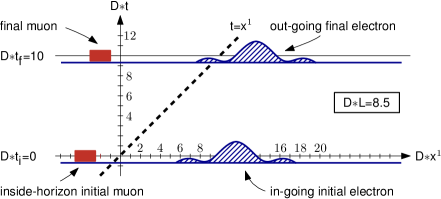
Figure 2: Sketch of an elastic electron-muon scattering process in Minkowski spacetime. The solid-red (striped-blue) profiles show the spatial support of the muon (electron) wave packets at initial time $t=t_{i}=0$ and final time $t=t_{f}=10/D$. The dashed line shows the projected black-hole horizon (cf. the Penrose diagram of Fig. 1). The initial muon is strictly localized within the projected black-hole horizon, while the initial electron, localized with large probability outside the projected black-hole horizon, is strictly localized in momentum space with finite support on negative $Q^{1}$ momenta (directed towards the black-hole center, left of the projected black-hole horizon in this figure). The final electron, localized with large probability outside the projected black-hole horizon, is strictly localized in momentum space with finite support on positive $Q^{1}$ momenta (directed away from the black-hole center).

3 Quantum scattering in Minkowski spacetime

3.1 Scattering probability amplitude without interactions

The probability amplitude corresponding to the scattering of the muon and the electron in the absence of interactions (coupling constant $\alpha=0$) reads

$$\mathcal{A}_{fi}^{(\alpha=0)} = \langle\psi_{X_{\mu,f},P_{\mu,f}}|\psi_{X_{\mu,i},P_{\mu,i}}\rangle\;\langle\psi_{X_{e,f},P_{e,f}}|\psi_{X_{e,i},P_{e,i}}\rangle\,,$$ (28a)

where

$$\langle\psi_{X_{\mu,f},P_{\mu,f}}|\psi_{X_{\mu,i},P_{\mu,i}}\rangle = {\int}d^{3}\mathbf{x}\,\big{(}\psi_{X_{\mu,f},P_{\mu,f}}(x)\big{)}^{\dagger}\;\psi_{X_{\mu,i},P_{\mu,i}}(x)$$ (28b)

$$={\int}\,\frac{d^{3}\mathbf{Q}}{(2\pi)^{3}}\,\big{(}F_{P_{\mu,f}}(\mathbf{Q})\big{)}_{\mu}\big{(}F_{P_{\mu,i}}(\mathbf{Q})\big{)}_{\mu}\,e^{-iQ{\cdot}(X_{\mu,f}-X_{\mu,i})}\,,$$

$$\langle\psi_{X_{e,f},P_{e,f}}|\psi_{X_{e,i},P_{e,i}}\rangle = {\int}d^{3}\mathbf{x}\,\big{(}\psi_{X_{e,f},P_{e,f}}(x)\big{)}^{\dagger}\;\psi_{X_{e,i},P_{e,i}}(x)$$ (28c)

$$={\int}\,\frac{d^{3}\mathbf{Q}}{(2\pi)^{3}}\,\big{(}F_{P_{e,f}}(\mathbf{Q})\big{)}_{e}\big{(}F_{P_{e,i}}(\mathbf{Q})\big{)}_{e}\,e^{-iQ{\cdot}(X_{e,f}-X_{e,i})}\;=\;0\,.$$

The last equality in (28c) is exact, because, for the chosen values of $P_{e,i}^{1}$, $P_{e,f}^{1}$, and $D$,

$$\text{rect}\left(\frac{Q^{1}-P_{e,f}^{1}}{2\,D}\right)\;\text{rect}\left(\frac{Q^{1}-P_{e,i}^{1}}{2\,D}\right) = 0\,,$$ (29)

and similarly for the spatial $2$ direction.

Thus, we have from (28a) and (28c), in the absence of interactions,

$$\mathcal{A}_{fi}^{(\alpha=0)} = 0\,.$$ (30)

This result is, of course, as expected: the initial electron has been designed to have only negative $Q^{1}$ momenta, so that, without interactions, there is zero overlap with a final electron having only positive $Q^{1}$ momenta.

Any detection of a final electron with positive $Q^{1}$ momentum requires nonzero momentum transfer, which, for the case of the interacting quantum-electrodynamics theory, traces back to the exchange of a virtual photon (cf. the Feynman diagram in Fig. 1). Indeed, if a final recoil electron is detected, this means that there must have been an interaction with a muon, at least for the setup considered.

We will now calculate the corresponding scattering probability amplitude. Incidentally, we may call this process “across-initial-muon-lightcone” scattering, as the recoil electron lies across (outside) the outmost lightcone of the initial muon wave packet; cf. Fig. 2.

3.2 Scattering probability amplitude with interactions

The probability amplitude for the scattering of the muon and the electron at the tree-level in perturbation theory of quantum electrodynamics (QED) reads [3, 4]

$$\mathcal{A}_{fi}^{\text{tree}} = \frac{i\alpha}{4\pi^{3}}{\int}d^{4}K\,\frac{\eta_{ab}\,J_{e}^{a}(K)J_{\mu}^{b}(K)}{\left(K-P_{\mu,f}+P_{\mu,i}\right)^{2}+i\epsilon}\,,$$ (31)

where $\epsilon$ is a positive infinitesimal and $\alpha\equiv e^{2}/4\pi$ the fine-structure constant. The currents $J_{e}^{a}$ and $J_{\mu}^{b}$ in (31) are defined as follows:

$$J_{e}^{a}(K) \equiv {\int}d^{4}x\,e^{-i(K-P_{\mu,f}+P_{\mu,i}){\cdot}x}\,$$ (32a)

$$\times\,\Big{[}\big{(}\bar{\psi}_{X_{e,f},P_{e,f}}(x)\big{)}_{e}\,\gamma^{a}\,\big{(}\psi_{X_{e,i},P_{e,i}}(x)\big{)}_{e}\Big{]}\,,$$

$$J_{\mu}^{b}(K) \equiv {\int}d^{4}x\,e^{+i(K-P_{\mu,f}+P_{\mu,i}){\cdot}x}\,$$ (32b)

$$\times\,\Big{[}\big{(}\bar{\psi}_{X_{\mu,f},P_{\mu,f}}(x)\big{)}_{\mu}\,\gamma^{b}\,\big{(}\psi_{X_{\mu,i},P_{\mu,i}}(x)\big{)}_{\mu}\Big{]}\,.$$

The integrand of (31) is nonvanishing and there is no obvious reason for the integral to give zero generically, that is, zero for all values of the distance parameter $L$ entering the boundary conditions (25) of the initial and final electron wave packets, for fixed boundary conditions (16) of the initial and final muon wave packets.

The multiple integral (31) cannot be computed analytically. Moreover, numerical calculation turns out to be nontrivial and time-consuming. We, therefore, make the approximation that the momentum variance $D$ is much smaller than the particle masses, i.e., $M_{e}/D\gg 1$ and $M_{\mu}/D\gg 1$. We then have

$$J_{e}^{a}(K) \approx E^{a}(K)$$ (33a)

$$\equiv {\int}d^{4}x\,\Big{[}\bar{e}_{X_{e,f},P_{e,f}}(x)\,\gamma^{a}\,e_{X_{e,i},P_{e,i}}(x)\Big{]}\,e^{-i(K-P_{\mu,f}+P_{\mu,i}){\cdot}x}\,,$$

$$J_{\mu}^{b}(K) \approx M^{b}(K)$$ (33b)

$$\equiv {\int}d^{4}x\,\Big{[}\bar{\mu}_{X_{\mu,f},P_{\mu,f}}(x)\,\gamma^{b}\,\mu_{X_{\mu,i},P_{\mu,i}}(x)\Big{]}\,e^{+i(K-P_{\mu,f}+P_{\mu,i}){\cdot}x}\,,$$

where $e_{X,P}(x)$ and $\mu_{X,P}(x)$ have been defined in (7) and (22). Explicitly, we obtain

$$E^{a}(K) = \frac{N_{e,f}N_{e,i}}{(\pi/D)^{6}}\,\Big{[}\bar{u}(P_{e,f})\,\gamma^{a}\,u(P_{e,i})\Big{]}\,e^{-iP_{e,f}{\cdot}X_{e,f}+iP_{e,i}{\cdot}X_{e,i}}{\int}d^{4}x\,e^{-iK{\cdot}x}$$ (34a)

$$\times\prod_{i=1}^{i=3}\text{sinc}\left[\frac{P_{e,f}^{i}\,\Delta{x}_{e,f}^{0}-P_{e,f}^{0}\,\Delta{x}_{e,f}^{i}}{P_{e,f}^{0}\big{/}D}\right]\,\text{sinc}\left[\frac{P_{e,i}^{i}\,\Delta{x}_{e,i}^{0}-P_{e,i}^{0}\,\Delta{x}_{e,i}^{i}}{P_{e,i}^{0}\big{/}D}\right],$$

$$M^{b}(K) = \frac{N_{\mu,f}N_{\mu,i}}{(2/D)^{6}}\,\Big{[}\bar{u}(P_{\mu,f})\,\gamma^{b}\,u(P_{\mu,i})\Big{]}\,e^{-iP_{\mu,f}{\cdot}X_{\mu,f}+iP_{\mu,i}{\cdot}X_{\mu,i}}{\int}d^{4}x\,e^{+iK{\cdot}x}$$ (34b)

$$\times\prod_{i=1}^{i=3}\text{rect}\left[\frac{P_{\mu,f}^{i}\,\Delta{x}_{\mu,f}^{0}-P_{\mu,f}^{0}\,\Delta{x}_{\mu,f}^{i}}{2P_{\mu,f}^{0}\big{/}D}\right]\,\text{rect}\left[\frac{P_{\mu,i}^{i}\,\Delta{x}_{\mu,i}^{0}-P_{\mu,i}^{0}\,\Delta{x}_{\mu,i}^{i}}{2P_{\mu,i}^{0}\big{/}D}\right].$$

Both integrals over $x$ can be evaluated analytically, the first with help of the formulae (3.742.6) and (3.742.8) in Ref. [5]. The obtained expressions are, however, cumbersome and will not be given here.

It should be noted that $E^{a}(K)$ has finite support. Specifically, $E^{a}(K)$ is nonvanishing if and only if

$$K^{0} \in \big{(}{-}\mathcal{K},\,+\mathcal{K}\big{)}\,,$$ (35a)

$$K^{i}/D \in \big{(}{-}2,\,+2\big{)}\,,$$ (35b)

where, in the first equation, we have taken into account the initial and final conditions (25) of the electron and where $$\mathcal{K}$$ is defined by

$$\mathcal{K} \equiv \left(\frac{P_{e,f}^{1}}{P_{e,f}^{0}}-\frac{P_{e,i}^{1}}{P_{e,i}^{0}}+\frac{P_{e,i}^{2}}{P_{e,i}^{0}}\right)D\;\approx\;2.393\;D\,.$$ (35c)

To summarize, we will evaluate the approximate amplitude

$$\mathcal{A}_{fi}^{\text{tree,\,approx}} \equiv \frac{i\alpha}{4\pi^{3}}{\int}d^{4}K\,\frac{\eta_{ab}\,E^{a}(K)\,M^{b}(K)}{\left(K-P_{\mu,f}+P_{\mu,i}\right)^{2}+i\epsilon}\,,$$ (36)

where $E^{a}(K)$ and $M^{b}(K)$ are given by (34) with all integrals over $x$ performed analytically. This approximation improves as the momentum variance $D$ drops to zero, specifically

$$\mathcal{A}_{fi}^{\text{tree,\,approx}}\to\mathcal{A}_{fi}^{\text{tree}}\,,\;\;\text{for}\;\;D/M_{e}\to 0\,,$$ (37)

where only the electron mass $M_{e}$ is shown for the $D$ limit, as the muon mass $M_{\mu}$ is larger than $M_{e}$. Note that $D$ is a naturally small parameter, because it must be negligibly small with respect to either the mass or the energy of the wave packets for them to propagate approximately like classical particles in special relativity.

3.3 Numerical results for the scattering probability amplitude

For the numerical evaluation of the scattering probability amplitude (36), we take the following parameter values:

$$M_{e}/D = 10\,,$$ (38a)

$$M_{\mu}/D = 2070\,,$$ (38b)

$$\alpha = 1/137\,,$$ (38c)

where the electron mass $M_{e}$ and the approximate muon mass $M_{\mu}\equiv 207\,M_{e}$ are considered to be fixed and $D$ is the momentum variance of the assumed wave packets of the initial and final particles. As a start, we have compared, for the numerical values (38) and the parameter value $L=8.5/D$ [entering the boundary conditions of the scattering process considered], the numerical result for the $J_{e}(K)\cdot J_{\mu}(K)$ numerator in the integrand of (31) with the analytic result for the $E(K)\cdot M(K)$ numerator in the integrand of (36), and find excellent agreement.

The results for the numerical evaluation of (36) are shown in Fig. 3. The rough order of magnitude of $10^{-11}$ for the amplitude in Fig. 3 can be understood as follows: the prefactor on the right-hand side of (36) gives a factor of order $10^{-4}$, the numerator at $K^{\mu}=0$ a factor of order $1$, and the denominator at $K^{\mu}=0$ a factor of order $10^{-7}$. Comparing different numerical calculations, we estimate the numerical accuracy of the results shown in Fig. 3 to be approximately $10^{-13}$.

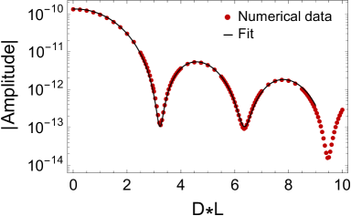
Figure 3: Absolute value of the scattering probability amplitude $\mathcal{A}_{fi}^{\text{tree,\,approx}}$ from (36) as a function of the distance $L$ entering the boundary conditions (16) and (25) [the initial and final wave functions involve the momentum variance $D$]. Numerical parameters (38) are used. The fit for $D\,L\in[0,\,9]$ is given by expression (39).

Purely empirically, we can fit the Fig. 3 numerical results for $D\,L\in[0,\,9]$ by the following even function:

$$\Big{|}\mathcal{A}_{fi}^{\text{tree,\,approx}}\big{(}D\,L\big{)}\Big{|}^{\text{(fit)}} = a_{0}\,\Big{|}\text{sinc}\left(D\,L-D\,\widetilde{\ell}_{0}\right)\Big{|}^{p_{0}}+b\big{(}D\,L\big{)}\,,$$ (39a)

$$\widetilde{\ell}_{0} = \frac{L}{\sqrt{\ell_{0}^{2}+L^{2}}}\;\ell_{0}\,,$$ (39b)

$$b\big{(}D\,L\big{)} = \frac{b_{0}}{1+b_{2}\,\big{(}D\,L\big{)}^{2}}\,,$$ (39c)

$$\big{\{}a_{0},\,\ell_{0},\,p_{0}\big{\}} \approx \left\{1.35{\times}10^{-10},\,0.084/D,\,2.12\right\},$$ (39d)

$$\big{\{}b_{0},\,b_{2}\big{\}} \approx \left\{1.05{\times}10^{-13},\,0\right\},$$ (39e)

where the function ‘sinc’ is defined by (6). A positive value of $b_{2}$ can perhaps be determined from better numerical data of the third dip at $D\,L\sim 3\,\pi$.

The nonzero result for the scattering probability amplitude (Fig. 3) implies that Minkowski-spacetime across-initial-muon-lightcone scattering as shown in Fig. 2 can take place in QED. As mentioned in Sec. 1, this implies, according to the Einstein Equivalence Principle, that across-horizon scattering is operative in a black-hole spacetime and we will discuss this further in the next section.

4 Across-horizon scattering for a massive black hole

In the present article, we have established, by explicit calculation, the nonzero probability for detecting a recoil electron in a special setup of elastic electron-muon scattering in Minkowski spacetime, where the recoil electron is detected outside the light-cone of the initial muon (Fig. 2). The setup is such that there is zero probability for detecting a recoil electron if there is no interaction taking place, which is the case if, for example, the initial muon is stopped by a closed shutter.

The Minkowski-spacetime result of a nonzero probability amplitude for a recoil electron (Fig. 3) provides the cap-stone of our previous argument [2] to establish the possibility of information transfer out of a Schwarzschild black hole. Indeed, a near-horizon spacetime region is approximately flat for a very massive black hole and this spacetime region with local inertial coordinates can be described by a patch of Minkowski spacetime (see Fig. 2 in Ref. [2]), where the original black-hole horizon projects on part of the light-cone in Minkowski spacetime (dashed line in Fig. 2). By the Einstein Equivalence Principle, the physics in this Minkowski-spacetime patch is described by standard QED [3, 4], if we consider electrically charged elementary particles and photons and omit the weak and strong interactions. Specifically, the flat-spacetime calculation of Sec. 3 is relevant for elastic electron-muon scattering in a near-horizon spacetime region of a Schwarzschild black hole with a sufficiently large mass ($M_{\text{BH}}\gg M_{P}^{2}\,c/D$, where $M_{P}^{2}\equiv\hbar c/G$ is the square of the Planck mass and $\hbar/D$ the characteristic quantum-particle size). See also App. B of Ref. [2] for further relevant numbers.

In Ref. [2], we have proposed a Gedankenexperiment that relies on the nonzero probability for a recoil electron, which is precisely what we have calculated in the present paper. A brief summary of this Gedankenexperiment is as follows. Two experimentalists, Castor and Pollux, meet outside the black-hole horizon to fix the procedure and also to establish a list of questions for Castor to answer. Castor then moves inside the black-hole horizon and starts the experiment at an agreed moment. While Pollux on the outside definitely sends out an appropriate bunch of electrons, Castor on the inside decides to send an appropriate bunch of muons if his answer to the first question is affirmative or decides not to send an appropriate bunch of muons if his answer to the first question is negative. Castor writes “yes” in his message-book if he sends the muons and “no” if he does not. The detector of Pollux is designed to record recoil electrons and Pollux writes “YES” in his logbook if there is at least one detected recoil electron and “NO” if there are no recoil electrons whatsoever. Hence, Castor’s yes/no answer to the first question is transmitted to Pollux, who reads YES/NO in his logbook. Castor and Pollux deal with further questions in the same way. Additional details and refinements can be found in Sec. 3 of Ref. [2].

To summarize, we have established that it is, in principle, possible to transmit a message (in binary code) from inside the black-hole horizon to outside the black-hole horizon by use of a quantum scattering process (Fig. 1). Another quantum process is, of course, spontaneous pair production, which plays a crucial role for the Hawking radiation of a black hole [6]. But it appears that this spontaneous pair-production process, in its simplest form, cannot be used to send a message from inside the black-hole horizon to outside. Still, even though the quantum scattering process can, in principle, be used to send such a message, it is not clear what this result implies for the so-called information-loss problem of black-hole physics [7].

References

• [1] C.W. Misner, K.S. Thorne, and J.A. Wheeler, Gravitation (Princeton University Press, Princeton NJ, USA, 2017).
• [2] V.A. Emelyanov and F.R. Klinkhamer, Across-horizon scattering and information transfer, Class. Quant. Grav. 35, 125004 (2018) [arXiv:1710.06405 [hep-th]].
• [3] R.P. Feynman, Space-time approach to quantum electrodynamics, Phys. Rev. 76, 769 (1949).
• [4] M.J.G. Veltman, Diagrammatica: The Path to Feynman Rules (Cambridge University Press, Cambridge, England, 1994).
• [5] I.S. Gradshteyn and I.M. Ryzhik, Table of Integrals, Series, and Products, Seventh Edition (Academic Press, San Diego CA, USA, 2007).
• [6] S.W. Hawking, Particle creation by black holes, Commun. Math. Phys. 43, 199 (1975), Erratum: Commun. Math. Phys. 46, 206 (1976).
• [7] W.G. Unruh and R.M. Wald, Information loss, Rept. Prog. Phys. 80, 092002 (2017) [arXiv:1703.02140 [hep-th]].