Identifying Transition States of Chemical Kinetic Systems using Network Embedding Techniques

Abstract

Using random walk sampling methods for feature learning on networks, we develop a method for generating low-dimensional node embeddings for directed graphs and identifying transition states of stochastic chemical reacting systems. We modified objective functions adopted in existing random walk based network embedding methods to handle directed graphs and neighbors of different degrees. Through optimization via gradient ascent, we embed the weighted graph vertices into a low-dimensional vector space ${\mathbb{R}}^{d}$ while preserving the neighborhood of each node. We then demonstrate the effectiveness of the method on dimension reduction through several examples regarding identification of transition states of chemical reactions, especially for entropic systems.

1 Introduction

Networks provide a natural framework for many chemical and biochemical systems, including chemical kinetics and dynamical interactions between biomolecules. The possible stages of a reaction, for example, can be viewed as vertices in a directed graph. Frequently, real-world networks are high-dimensional and complex in structure, which leads to difficulties in interpretation and analysis. In order to take full advantage of the structural information contained in such networks, efficient and robust methods of effective network analysis are essential to produce low dimensional representations while retaining principal correlations of the graph.

Networks analysis is especially useful for understanding behaviors of nonlinear chemical processes such as biochemical switches. Biochemical switches are systems of chemical reactions with multiple steady states. Without random perturbations, the system will spend all its time at the metastable states, where energy is minimized, while the presence of stochastic noise in the dynamics can lead to transitions between metastable states. Difficulties arise in the simulation of such systems as a result of the multiple time scales at work; transitions between steady states are typically rare, but occur rapidly.

The different possible states of the reaction, given by the varying concentrations of reactant and product species, can be viewed as the vertices of a weighted directed graph. The progression of the reaction over time can then be viewed as a Markov jump process, where the jump probabilities are represented by the weights on the edges between each pair of nodes. Then, methods for network analysis can be used to identify interactions and pathways between the components of the biochemical switch. One objective of this paper is to suggest a method to analyze this Markov process using node embedding techniques. This paper will focus on the $A\to B$ problem: $A$ and $B$ are taken as the reactant and product states, respectively. The aim of this paper is to investigate the mechanism by which this transition occurs.

Recently, methods for analyzing networks through feature representation and graph embedding have received increasing attention. For an overview on this subject, a number of recent review papers are available [14, 7]. While much of this research has been focused on undirected graphs, the directed case has also been investigated, for example [10, 9, 24]. In particular, several methods have been proposed that utilize random walks for node embedding.

Node embedding (or feature learning) methods aim to represent each node of a given network as a vector in a low-dimensional continuous vector space, in such a way that information about the nodes and relationships between them are retained. Specifically, nodes that are similar to each other according to some measure in the original graph will also have similar representations in the embedding space. Usually, this means that the embedding will be chosen in a way that maximizes the inner products of embedding vectors for embedded nodes that are similar to each other. Compared with the original complex high-dimensional networks, these low dimensional continuous node representations have the benefit of being convenient to work with for downstream machine learning techniques.

Compared with alternative methods that embed edges or entire graphs instead of nodes, node embeddings are more adaptive for numerous tasks, including node classification, clustering, and link prediction [7]. Node classification is a process by which class labels are assigned to nodes based on a small sample of labelled nodes, where similar nodes have the same labels. Clustering algorithms group the representations of similar nodes together in the target vector space. Link prediction seeks to predict missing edges in an incomplete graph.

The recent interest in feature learning has led to a collection of different node embedding methods, which can be broadly classified [14] by the analytical and computational techniques employed such as matrix factorization, random walk sampling, and deep learning network. The matrix factorization based methods generate embeddings by first using a matrix to represent the relationships between nodes, which include the Laplacian matrix as in the Laplacian eigenmaps [3], the adjacency matrix as in locally linear embedding (LLE) [20] or graph factorization (GF) [1], etc. Though the above methods focus on the case of undirected methods, similar techniques for the directed case have also been suggested [10], where the development of the Laplacian matrix, a combinatorial Laplacian matrix, and Cheeger inequality allow the above approaches to be extended for directed graphs. Factorization based methods such as eigenvalue decomposition can apply for certain matrices (e.g. positive semidefinite), and additional difficulties may arise with scaling for large data sets.

Random walk methods are often used for large graphs, or graphs that cannot be observed in their entirety. The general idea involves first simulating random walks on a network, then using the output to infer relationships between nodes. Random walk methods can be used to study either undirected or directed graphs, although much of the previous work has focused on the undirected case. For example, DeepWalk [19] uses short unbiased random walks to find similarities between nodes, with node pairs that tend to co-occur in the same random walks having higher similarities. This method performs well for detecting homophily – similarity based on node adjacency and shared neighbors. Similar methods, such as node2vec [15], use biased random walks to capture similarity based on both homophily and structural equivalence – similarities in the nodes’ structural roles in the graph. Both of these methods specifically address undirected graphs. A similar approach designed for the directed case is proposed in [9], which uses Markov random walks with transition probabilities given by ratios of edge weights to nodes’ out degrees, together with the stationary distribution of the walks, to measure local relationships between nodes.

Theoretical frameworks for the study of transition events of biochemical processes include Transition State Theory (TST), Transition Path Sampling (TPS), Transition Path Theory (TPT) and Forward Flux Sampling (FFS). The main idea of TST is that in order for the system to move from the reactant state to the product state, the system must pass through a saddle point on the potential energy surface, known as a Transition State [4]. The TPS technique uses Monte Carlo sampling of transition paths to study the full collection of transition paths of a given Markov process [5]. Transition Path Theory (TPT) studies reactive trajectories of a system by considering statistical properties such as rate functions and probability currents between states [6]. Forward flux sampling [2], designed specifically to capture rare switching events in biochemical networks, uses a series of interfaces between the initial and final states to calculate rate constants and generate transition paths. For the purpose of this paper, we will be using TPT, but other such techniques can fit into the method presented here as well.

This paper will suggest a method of using a random walk network embedding approach for node classification and clustering on directed graphs, as well as identification of transition states for the specific case of entropy effects. The method presented reduces the dimension of networks, thereby allowing analysis and interpretation of the system. First, in Section 2 we will introduce some background regarding feature learning on networks, and provide a brief overview of some basic principles from TPT. Then Section 3 will introduce a method for node classification for directed graphs, based on random walk node embedding. Finally, in Section 4, we will study several examples, showing the effectiveness of the method on identifying transition states of entropic systems.

2 Background

In this paper, we focus on the mechanism by which a system such as a biochemical switch passes through its energy landscape following a reactive trajectory. A trajectory is said to be reactive if it leaves the reactant state $A$ and later arrives at the product state $B$ without first returning to state $A$. Such a trajectory can be viewed as a sequence of transitions between metastable states where the energy is locally minimized. In particular, we treat these sequences as Markov jump processes, and study the probability space of these reactive trajectories in order to identify and understand the transition events of the system.

Though this paper will be utilizing the techniques of Transition Path Theory for this purpose, it is also possible to adopt other frameworks, such as Transition Path sampling, Forward Flux sampling, etc., to investigate the transition events of a system. As a Monte Carlo technique, Transition path sampling [5] is essentially a generalization of importance sampling in trajectory space. The basic idea is to perform a random walk in trajectory space, biased so that important regions are visited more often. Forward flux sampling (FFS) [2], which generates trajectories from $A$ to $B$ using a sequence of nonintersecting parametrizable surfaces, has the advantage that knowledge of the phase space density is not required.

Consider a Markov jump process on a countable state space $S$. Let $L=(l_{ij})_{i,j\in S}$ represent the infinitesimal generator of the process. In other words, for $i\neq j$, $l_{ij}\Delta t+o(\Delta t)$ represents the probability that a process that is in state $i$ at time $t$ will jump to state $j$ during the time interval $[t,t+\Delta t]$. Then the entries of $L$ are transition rates, satisfying

$$\begin{cases}l_{ij}\geq 0\hskip 7.22743pt&\forall\ i,j\in S,\ i\neq j,\\ \sum_{j\in S}l_{ij}=0,\hskip 7.22743pt&\forall\ i\in S.\\ \end{cases}$$ (2.1)

Let $\{X(t)\}_{t\in{\mathbb{R}}}$ represent an equilibrium sample trajectory of the Markov process, such that $\{X(t)\}_{t\in{\mathbb{R}}}$ is right-continuous with left limits. At time $t$, let the probability distribution of this process be denoted by $\mu(t):=(\mathbb{P}(X(t)=i))_{i\in S}^{T}$. Then the time evolution of $\mu(t)$ follows the forward kolmogorov equation (or master equation)

$$\frac{d\mu}{dt}=\mu^{T}L\text{,}\quad t\geq 0.$$

Denote the time-reversed process by $\{\tilde{X}(t)\}_{t\in{\mathbb{R}}}$, and the infinitesimal generator of this process by $\tilde{L}$. The stationary probability distribution of both processes, $\{X(t)\}_{t\in{\mathbb{R}}}$ and $\{\tilde{X}(t)\}_{t\in{\mathbb{R}}}$ $\pi=(\pi_{i})_{i\in S}$, is given by the solution to

$$0=\pi^{T}L\ .$$

2.1 Network Embedding for Directed Graphs

Networks can have large numbers of vertices and complex structures, which can lead to challenges in network analysis. To overcome these difficulties and improve understanding of these networks, the nodes of a given network can be embedded into a low-dimensional vector space, a process called feature learning. The techniques used in this paper to investigate transition states and pathways is a combination of neural network-based and random walk-based methods for learning latent representations of a network’s nodes, as discussed in [15, 19, 9]. The idea behind these methods is that the nodes in a given network $G=G(V,E)$ can be embedded into a low-dimensional vector space in such a way that nodes similar to each other according to some measure in the original graph will also have embeddings similar to each other in the embedding space.

Feature learning, or node embedding, requires three main components: an encoder function, a definition of node similarity and a loss function. The encoder function is the function that maps each node to a vector in the embedding space. To find the optimal embeddings, the encoder function can be chosen by minimizing the loss function so that the similarity between nodes in the original network corresponds as close as possible to the similarity between their vector representations in the continuous space. Node similarity can have different interpretations, depending on the network and the task to be accomplished. For example, nodes that are connected, share neighbors, or share a common structural role in the original graph can be claimed to be similar, and to be embedded in the vector space by representations of close similarity. For the embedded vectors, a common approach is to use inner products as the similarity measure in the feature space–that is, if $u$ and $v$ are two nodes in a graph with representations $z_{u}$ and $z_{v}$ in a low-dimensional vector space, then $z_{u}^{T}z_{v}$ should approximate the similarity between representations $z_{u}$ and $z_{v}$.

2.1.1 Factorization Approaches

Many feature learning methods obtain node embeddings via factorization of a matrix containning information regarding relationships between nodes. Locally Linear Embedding (LLE) [20] and Graph Factorization (GF) [1], utilize the node adjacency matrix entry $A_{i,j}$ being the weight of edge $(i,j)$ in the graph. Laplacian Eigenmaps and related methods instead factorize the Laplacian matrix of the whole graph. Optimization of the loss function is typically solve as an eigenvalue problem.

While the methods mentioned here mainly preserve first-order node relationships, i.e., two nodes that are directly connected by an edge are similar, other factorization methods such as GraRep, Cauchy graph embedding and structure preserving embedding can detect higher-order relationships between nodes, or alternative notions of similarity such as structural equivalence [8, 14, 7].

2.1.2 Random Walk Approaches

One technique for finding node embeddings is through the use of random walks. This technique has been applied to undirected graphs in methods such as DeepWalk and node2vec [19, 15]. In these methods, the general approach is to use short random walks to determine similarities for each pair of nodes. The notion of node similarity is co-occurence within a random walk; two nodes are similar if there is a higher probability that a walk containing one node will also contain the other. The various methods using this approach differ in the implementation of this general idea: DeepWalk, for example, uses straightforward unbiased walks, while node2vec uses adjustable parameters to bias random walks toward breadth-first or depth-first sampling for a more flexible notion of similarity.

The first stage in the feature learning process is to simulate a certain number of random walks starting from each vertex. Using the results of these random walks, the neighbors of each node can be determined. The objective is to maximize the probability of observing the neighborhood of each node, conditioned on the vector representation of the node. In several of the random walk-based feature representation methods for undirected graphs, this is achieved through the Loss function of the form:

$$\max_{e}J(e)\ =\ \sum_{u\in V}\log Pr(N_{S}(u)|e(u)),$$ (2.2)

where $V$ is the set of all vertices in the graph, $N_{S}(u)$ is the neighborhood of the node $u$, and $e(u)$ is the encoder function representating the embedded vector. If we assume that the probabilities of observing a particular neighbor are independent, we can have

$$Pr(N_{S}(u)|e(u))=\prod_{n_{i}\in N_{S}(u)}Pr(n_{i}|e(u)).$$ (2.3)

Since these methods typically aim to maximize the inner products for neighboring nodes, they often utilize a softmax function to model each conditional probability:

$$Pr(n_{i}|e(u))=\frac{\exp\big{(}e(n_{i})\cdot e(u)\big{)}}{\sum_{v\in V}\exp\big{(}e(v)\cdot e(u)\big{)}}\ .$$

For networks where $|V|$ is large, techniques such as hierarchical softmax [19] or negative sampling [18] can be used to increase efficiency. To determine the optimal embedding function $e(u)$, the Loss function can be optimized using gradient ascent respect to parameters of $e(u)$.

In [9], a random walk-based method specifically intended for directed graphs is proposed. The function to be optimized in this method, when embedding into ${\mathbb{R}}^{1}$, is

$$I=\sum_{u}\pi_{u}\sum_{v,u\to v}p(u,v)(y_{u}-y_{v})^{2},$$

where $y_{u}$ is the one-dimensional embedding of $u$, $\pi_{u}$ is the stationary probability for the node $u$ and $p(u,v)$ represents the random walk’s transition probability from $u$ to $v$. The transition probabilities are calculated according to

$$p(u,v)=w(u,v)/\sum_{k,u\to k}w(u,k),$$

where $w(u,v)$ is the weight on the edge $(u,v)$. Note that this method, though it uses transition probabilities of a random walk, does not actually require simulation of random walks, since all the summations can be done deterministically.

According to the spectral graph theory [10], a circulation on a directed graph is a function $F$ such that, for each $u\in V$, $\sum_{u,u\to v}F(u,v)=\sum_{w,v\to w}F(v,w)$. The Laplacian of a directed graph is therefore defined as

$$\mathcal{L}=I-\frac{\Phi^{1/2}P\Phi^{-1/2}+\Phi^{-1/2}P\Phi^{1/2}}{2},$$

where $\Phi$ is a diagonal matrix with diagonal entries given by $\Phi(v,v)=\phi(v)=\sum_{u,u\to v}F(u,v)$ for some circulation function $F$. The following definition of the combinatorial Laplacian is also due to Chung[10]:

$$\mathbb{L}=\Phi-\frac{\Phi P+P^{T}\Phi}{2},$$

where $P$ is the transition matrix, i.e. $P_{ij}=p(i,j)$, $\Phi$ is the diagonal matrix of the stationary distribution, i.e. $\Phi=diag(\pi_{1},\dots,\pi_{n})$. Note that the combinatorial Laplacian is symmetric and semi-positive definite. It is shown in [9] that

$$\sum_{u}\pi_{u}\sum_{v,u\to v}p(u,v)(y_{u}-y_{v})^{2}=2y^{T}\mathbb{L}y$$

where $y=(y_{1},y_{2},\dots,y_{n})^{T}$. This result demonstrates that this method is analogous to the Laplacian-based methods for undirected graphs, e.g. Laplacian eigenmaps [14].

Random walk methods have been shown to perform well compared to other methods, and can be useful for a variety of different notions of node similarity. Previous work has shown them to be robust, efficient, and capable of completing a diverse range of tasks, including node classification, link prediction, clustering, and more [14, 7, 19, 15]. Because they do not examine the entire graph at once, these methods are also useful for very large networks and networks that cannot be observed in their entirety.

2.1.3 Neural Network Approaches

A third class of graph embedding methods involves the use of deep learning techniques, including neural networks [7, 14], e.g. Graph Neural Network (GNN) [7, 21]. Such methods have been shown to perform well, particularly for dimension reduction and identifying nonlinear relationships among data. Random walk based methods, such as DeepWalk, can incorporate deep learning algorithms like SkipGram for graph embedding, where random walks serve to provide neighborhood information as input.

In general, neural network methods typically work by assigning a weight to each node representation, and then combining those terms via a transfer function. This result is then used as the input for an activation function, such as a sigmoid function, i.e. $\sigma(x)=1/(1+\exp(-x))$. This process may then repeat for multiple layers. In a neural network method, the parameters to be optimized are the weights, which are updated after each layer, typically by gradient descent. In the GNN [21], the objective function to be minimized is of the form

$$W=\sum_{i}\sum_{j}(t_{i,j}-\varphi_{w}(G_{i},n_{i,j}))^{2},$$

where $G_{i}$ is the learning set, the $n_{i,j}$ and $t_{i,j}$ are the nodes and target outputs, and the goal is to choose the parameter $w$ in such a way that $\varphi$ closely approximates the target outputs. This optimization occurs through gradient descent, where the gradient is computed with respect to the weights $w$.

2.2 Transition Path Theory

In order to identify the transition paths of a given Markov process, we will adopt the framework of Transition Path Theory (TPT). The following notations are mostly from [17]. Consider a state space $S$, for an initial state $A\in S$ and final state $B\in S$, a trajectory $X(t)$ is said to be reactive if it begins from state $A$ and reaches at state $B$ before returning to state $A$.

To determine whether a given reaction path is reactive, we will need the following forward and backward committor functions. For each $i\in S$, the forward committor $q_{i}^{+}$ is the probability that a process initially at state $i$ will reach state $B$ before it reaches state $A$. Similarly, the discrete backward committor $q_{i}^{-}$ denotes the probability that a process arriving at state $i$ was more recently in state $A$ rather than in state $B$. The forward committors satisfy the following Dirichlet equation

$$\begin{cases}\sum_{j\in S}l_{ij}q_{j}^{+}&=0\hskip 36.135pt\forall i\in(A\cup B)^{C}\\ q_{i}^{+}&=0\hskip 36.135pt\forall i\in A\\ q_{i}^{+}&=1\hskip 36.135pt\forall i\in B,\\ \end{cases}$$

and similar equations are satisfied by backward committors.

The probability current, or flux, of reactive trajectories gives the average rate at which reactive paths transition from state to state. For trajectories from $A$ to $B$, the probability current is defined for all $i\neq j$ such that

$$f_{ij}^{AB} =\lim_{s\to 0+}\frac{1}{s}\lim_{T\to\infty}\frac{1}{2T}\int_{-T}^{T}\mathbf{1}_{\{i\}}(X(t))\mathbf{1}_{\{j\}}(X(t+s))\times\sum_{n\in{\mathbb{Z}}}\mathbf{1}_{(-\infty,t_{n}^{B}]}(t)\mathbf{1}_{[t_{n}^{A},\infty)}(t+s)dt$$

$$=f^{AB}_{ij}.$$

Also, for all $i\in S$, $f^{AB}_{ii}=0$. It can be shown that

$$f^{AB}_{ij}=\left\{\begin{array}[]{lll}\pi_{i}q_{i}^{-}l_{ij}q_{j}^{+},&\text{if }i\neq j\\ 0&\text{if }i=j.\\ \end{array}\right.$$

Since we are primarily interested in the flow from $A$ to $B$, and the process can move in either direction between two adjacent nodes on the path, the following effective current accounts for the net average number of reactive paths that jump from $i$ to $j$ per time unit:

$$f_{ij}^{+}=\max(f_{ij}^{AB}-f_{ji}^{AB},0).$$

We can also define the total effective current for a node $i$:

$$C_{i}^{+}=\sum_{j:(i,j)\in E}f_{ij}^{+}.$$

In [11], the effective current is generalized to a connected subnetwork of nodes $\Omega$ such that

$$C^{+}(\Omega)=\sum_{i\in\partial\Omega}C_{i}^{+},$$

which leads to the following definition of transition states of a time reversible process as subsets of the state space:

$$TS=\lim_{\sigma\to 0}\underset{\Omega}{\mathrm{argmax}}\{C^{+}(\Omega)\exp\left(-(q^{+}-0.5)^{2}/\sigma^{2}\right)\}$$

For the non-time reversible case, transition states can be identified similarly, replacing the exponential argument $\left(-(q^{+}-0.5)^{2}/\sigma^{2}\right)$ with $(-(q^{+}-0.5)^{2}+(q^{-}-0.5)^{2})/\sigma^{2}$. The above definition gives the flexibility of identifying transition states as subsets of the states space, which will be very useful when dealing with complex dynamics such as entropy effects.

3 Identifying Transition States using Network Embedding

We now introduce a method to identify transition states and paths of Markov processes, by random walk based Network Embedding techniques for directed networks. Consider a Markov jump process in a countable state space $S$. Using the infinitesimal generator $L$ for the process, we can calculate the stationary probability distribution $\pi$ and the forward and backward committors, based on which probability current and effective currents $f_{ij}^{AB}$ and $f_{ij}^{+}$ can then be computed. Once these quantities have been obtained, the discretized state space can be viewed as a weighted, directed graph $G(V,E)$. The nodes $v\in V$ are the grid points representing states of the system, and each pair of adjacent nodes are connected by an edge $(u,v)\in E$ with weights given by the effective probability current, such that the direction of the edge will be determined by the sign of the effective current.

Once $G$ is constructed, we can apply feature learning techniques for node classification to identify transition states. Random walk trials for similarities between nodes will start from each node in the space, using the edge weights as transition probabilities. The outputs of the random walks can then be used to compute experimental “neighbor probabilities”, i.e., the probability that a random walk of length $d$ starting at node $m$ will contain node $n$. If the neighbor probability for a node pair $(n,m)$ is sufficiently high, then the node $n$ is claimed as a neighbor of $m$. Note that this is a directed process; $n$ can be a neighbor of $m$ even if $m$ is not a neighbor of $n$.

After finding these conditional probabilities and identifying the neighborhoods of each node, the next step is to maximize an objective function in order to solve for the node embeddings. As in the node2vec and DeepWalk methods for the undirected case, the conditional probabilities are modeled using softmax functions. In order to adapt this technique for the case of directed graphs, we will use a modified version of the objective function:

$$V[e]=\sum_{u}\pi_{u}\sum_{v\in N(u)}Pr(v|e(u)).$$ (3.1)

Optimizing this function will give the encoder function $e^{opt}$ that maximizes the probability of the neighborhood of each node, with the most relevant nodes having the most influence on the feature representations.

In the original form of the objective function (3.1) for the undirected graph methods described above, the softmax functions depend only on whether nodes are neighbors, and is independent of the probability (frequency) that a particular neighbor will show up in a random walk trial. In other words, all neighbors are treated equally, while in reality some node pairs are more likely to co-occur than others. To address this, the objective function used here incorporates the neighboring probabilities, denoted $NP(\cdot,\cdot)$ such that

$$Pr(n_{i}|e(u))=\frac{\exp(e(n_{i})\cdot e(u))NP(n_{i},u)}{\sum_{v\in V}\exp(e(v)\cdot e(u))NP(v,u)}.$$

Algorithm 1 A random walk simulation method for directed graphs, given the transition matrix $t$.

  for $u\in V$ do

     $walk(1)=u$

     for  $step=1:walklength$ do

        for  $k=2:d$ do

           $total=\sum_{v,walk(k-1)\to v}t(walk(k-1),v)$

           for  $v:walk(k-1)\to v$ do

              $P(walk(k-1),v)=t(walk(k-1),v)/total$

           end for

           Use probability $P(walk(k-1),\cdot)$ to choose $walk(k)=v$ for some neighbor of $walk(k-1)$.Set $counter(walk(k),u)=counter(walk(k),u)+1$.

        end for

     end for

  end for

  for $u,v\in V$ do

     $neighborprobability(u,v)=counter(u,v)/\sum_{k}counter(u,k)$

  end for

Assuming $e(u)=E_{2}u$, for $E_{2}$ being a $2\times d$ matrix, the objective defined above can then be maximized using gradient ascent to obtain the matrix $E_{2}^{opt}$ and therefore the feature embeddings. In practice, the linear assumption on the map from nodes to embeddings appears to be insufficiently flexible, particularly for higher-dimensional problems. To improve upon this, a neural network can be incorporated into the feature learning process, with the sigmoid function $\sigma(u)=1/(1+\exp(-e(u)))$ where $e(u)$ is the representation in the embedding space of the node $u$. The current algorithm uses a relatively small number of layers; raising this number results in node representations that are clustered more closely to their neighbors.

To obtain transition states for a particular process, we will examine the similarities between the node representations of each state and representation of metastable state $A$. Here, by “similarities” we mean the conditional probabilities given by the softmax units discussed previously. By construction, these values will naturally be small for nodes that are further from node $A$, due to hopping distances that are longer than the length of the random walks. So, to find the transition states, we combine similarities of node pairs with shorter hopping distances via matrix propagation, e.g.

$$sim(A,u)=\sum_{A\to v,v\to u}sim(A,v)*sim(v,u).$$ (3.2)

Note that a node $u$ for which this value is high is a higher-order neighbor of the reactant node $A$; therefore, such a node will have a higher probability of lying along a transition path. We then define transition states as nodes with high probability of lying on a transition path, which are not direct neighbors of the reactant or product states.

4 Examples and Results

Next, we will illustrate the suggested method on several simple examples. In the examples presented here, we have used $100$ random walk trials, each of length $9$ steps. Smaller numbers of trials increase the impact of noise in the results. Due to the matrix propagation technique described above, changes to the walk length parameter do not have a noticeable affect.

4.1 Diffusion Process with Energy Barrier

Figure 1: Diffusion process with energy barrier: plot assigning colors to each node in the discretized domain $\Omega$, according to each node’s similarity to the starting node $A$. Higher similarity values correspond to higher dot products between the two-dimensional embeddings of the nodes. The left plot corresponds to a parameter value of $\varepsilon=0.01$, while the right plot corresponds to $\varepsilon=1$.

Figure 2: Feature representations of nodes with high similarity to the reactant state $A$ for the 2D diffusion process with energy barrier, with $\varepsilon=0.01$.

First we will consider a two-dimensional diffusion process representing the position of a particle which follows the SDE

$$\frac{dx}{dt} =-\frac{dV}{dx}+\frac{dW_{1}(t)}{dt},$$

$$\frac{dy}{dt} =-\frac{dV}{dy}+\frac{dW_{2}(t)}{dt},$$

where $V$ is the potential

$$V=(x^{2}-1)^{2}+\varepsilon y^{4},$$ (4.1)

and $W_{1}(t)$ and $W_{2}(t)$ are independent Brownian motion processes.

This potential $V$ has two metastable states, or local minima, at (-1,0) and (1,0), as well as a saddle point at the origin. Here I will take (-1,0) to be the reactant state $A$, and (1,0) to be the product state $B$. The diffusion process can be approximated using a Markov (birth-death) jump process on a discrete state space. For this example, we will study the diffusion process on the domain $\Omega=[-1,1]\times[-0.75,0.75]$ by examining the Markov jump process on a grid $D=((-1+h{\mathbb{Z}})\times(-0.75+h{\mathbb{Z}}))\cap\Omega$, with $h=0.05$.

In order to examine the behavior of this Markov process, we should first compute the probability currents for the process. The infinitesimal transition matrix $L$ can be found by using the jump rates for the birth-death process $l_{nm}$ for each pair of adjacent nodes $n,m$ [12]. We define the following constants for a state $(x,y)\in(a,b)$:

$$k_{x}^{+}(x,y) =1/(2*h^{2})-1/(2*h)*dVdx(x-h),$$

$$k_{x}^{-}(x,y) =1/(2*h^{2})+1/(2*h)*dVdx(x+h),$$

$$k_{y}^{+}(x,y) =1/(2*h^{2})-1/(2*h)*dVdy(y-h),$$

$$k_{y}^{-}(x,y) =1/(2*h^{2})+1/(2*h)*dVdy(y+h).$$

Also let $k_{x}^{+}(x+h,y)=1/h$ if $x=A$, $\ k_{x}^{+}(x+h,y)=0$ if $x=B$, and $k_{x}^{-}(x-h,y)=0,\ k_{x}^{-}(x-h,y)=1/h$ if $x=A$ or $x=B$ respectively, and similarly for $k_{y}^{+}$ and $k_{y}^{-}$. Then the infinitesimal generator can be expressed in terms of its action on a test function $f$ such that

$$(Lf)(x,y)= k_{x}^{+}(x+h,y)(f(x+h,y)-f(x,y))+k_{x}^{-}(x-h,y)(f(x-h,y)-f(x,y))$$

$$+k_{y}^{+}(x,y+h)(f(x,y+h)-f(x,y))+k_{y}^{-}(x,y-h)(f(x,y-h)-f(x,y)).$$

Figure 1 assigns each point in the grid a color based on its similarity to the node of $A=(-1,0)$, for epsilon values $\varepsilon=.01$ and $\varepsilon=1$ in equation (4.1), respectively. To account for the fact that nodes with greater hopping distances from $A$ will have lower similarities to this node, we propagate the similarity matrix according to (3.2) in order to assign similarities to more distant nodes. The red area passing from $A$ to $B$ represents the region that reactive trajectories will pass through with the highest probability for each value of epsilon.

In Figure 2, the node embeddings $(u,v)=e_{opt}(x,y)$ corresponding to a subset of nodes with higher similarity values to $A$ are shown, for the case where $\varepsilon=0.01$, where $e_{opt}$ is the optimal linear encoding. Notice that in this figure, the embeddings for nodes with the highest probability of occurring in a reactive trajectory are clustered together, while nodes with lower probabilities tend to be grouped with other nodes with similar probabilities; more specifically, nodes with similarity values in the range $0.5-0.6$ have embeddings clustered near the upper left or lower right of the figure, while nodes with values from $0.7-0.8$ will have embeddings which appear in one of the two orange clusters.

In the context of the diffusion process with the potential $V$, the entropy effect refers to changes in the system’s observed dynamics in response to the change of the parameter $\varepsilon$. That is, as $\varepsilon$ is decreased, $dV/dy$ shrinks and therefore the negative term of $dy/dt$ becomes small. As a result, the shape and size of the saddle point located at the origin is altered, and we can expect the y-coordinate to take on a greater variety of values with higher probabilities in this case. In particular, around the origin, smaller values of $\varepsilon$ should result in higher similarities between the nodes above and below the origin, since in this case the process is more likely to move up and down. For larger values of $\varepsilon$, the process is expected to move straight forward from $A$ to $B$, with a smaller probability of moving up or down.

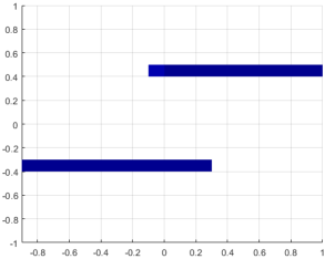
Figure 3: Diffusion process with entropic bottleneck: surface plot of the similarity function between the reactant state $A$ and nodes in $\Omega$. Here, the discretization with $h=0.1$ is used.

4.2 Diffusion Process with Barriers

Figure 4: Feature representations of nodes with high similarity to the reactant state $A$ for the entropic diffusion process.

Next we consider a pure diffusion process ($V(x,y)=0$) on the domain $\Omega=[-1,1]\times[-1,1]$ with two barriers as depicted in Figure 3. This example was also discussed in [16]. Here we take the node at $(0.6,0.6)$ to be the initial state $A$, and $(-0.6,-0.6)$ as the final state $B$. The particle spends most of its time between the reactant and product states, in the region between the barriers ($[-1,1]\times[-0.4,0.4]$). The only factor affecting the probability that the particle will reach $B$ before returning to $A$ is its current distance to $B$, since there are no energetic obstacles to overcome. In order to travel from $A$ to $B$, the process must find its way past the obstacles by chance, thereby overcoming an entropic barrier.

Figure 4 shows the node embeddings for a subset of nodes with high similarity values to reactant $A$. Note that the color scheme used in this figure corresponds to the color scheme in Figure 3; node embeddings that are colored red in the scatter plot correspond to red areas in the surface plot. In Figure 4, node embeddings again tend to be grouped by the corresponding values of the similarity function: nodes that are very similar to the initial state $A$ (similarity function value $>0.9$) appear in the red cluster toward the lower right. Other clusters of different colors correspond to groups of nodes with lower probabilities of appearing in a reactive trajectory. The yellow cluster contains embeddings of nodes with similarity function values approximately $0.7-0.8$, while the blue cluster corresponds to nodes with similarity values near $0.5-0.6$.

4.3 Three-Dimensional Toggle Switch

Now we will consider a higher-dimension example, a stochastic model of a 3D genetic toggle switch consisting of three genes that each inhibit the others’ expression [11]. We consider the production and degradation of the three gene products, $S_{1},S_{2},$ and $S_{3}$:

$$*\underset{\alpha_{4}}{\stackrel{{\scriptstyle\alpha_{1}}}{{\rightleftharpoons}}}S_{1},*\underset{\alpha_{5}}{\stackrel{{\scriptstyle\alpha_{2}}}{{\rightleftharpoons}}}S_{2},*\underset{\alpha_{6}}{\stackrel{{\scriptstyle\alpha_{3}}}{{\rightleftharpoons}}}S_{3},$$

where the parameters $\alpha_{i}$ are defined:

$$\alpha_{1}=\frac{c_{11}}{(65+x_{2}^{2})(65+x_{3}^{2})}\ , \alpha_{2}=\frac{c_{12}}{(65+x_{1}^{2})(65+x_{3}^{2})}\ ,$$

$$\alpha_{3}=\frac{c_{13}}{(65+x_{1}^{2})(65+x_{2}^{2})}\ , \alpha_{4}=c_{4}x_{1}\ ,$$

$$\alpha_{5}=c_{5}x_{2}, \alpha_{6}=c_{6}x_{3},$$

with $c_{11}=2112.5$, $c_{12}=845$, $c_{13}=4225$, $c_{4}=0.0125$, $c_{5}=0.005$, and $c_{6}=0.025$. From the stationary probability distribution, it can be seen that this model has three metastable states:

$$A=\{x\in S |35\leq x_{1}\leq 45,0\leq x_{2}\leq 4,0\leq x_{3}\leq 4\},$$

$$B=\{x\in S |35\leq x_{2}\leq 45,0\leq x_{1}\leq 4,0\leq x_{3}\leq 4\},$$

$$C=\{x\in S |35\leq x_{3}\leq 45,0\leq x_{2}\leq 4,0\leq x_{1}\leq 4\}.$$

Here we will choose $A$ to be the reactant state and $B$ to be the product state.

Figure 5: Surface plot of the similarities to $A$ of grid points in the domain $\Omega$ for the 3-D Toggle switch model. Results are for a $15\times 15\times 15$ discretization ($h=3$).

Figure 5 assigns colors to each node in $\Omega=\{ih,jh,kh|i,j,k\in{\mathbb{Z}}\}\cap[0,45]\times[0,45]\times[0,45]$ based on their similarity to node sin $A$, propagating the similarity matrix for nodes with larger hopping distance from $A$ as described previously. This figure shows two potential transition states for this system. A reactive trajectory from $A$ to $B$ will be most likely to pass directly from $A$ to $B$ along the higher-probability trajectory, represented in red. However, such a trajectory may instead reach $B$ after travelling through state $C$, as indicated by the fainter region connecting $A$ and $B$ via $C$.

Below, Figure 6 shows the two-dimensional node embeddings in ${\mathbb{R}}^{2}$, with the embeddings of nodes with zero similarity to $A$ omitted for clarity. There are several distinct clusters present in Figure 6, each representing a cluster of similar nodes. The nodes with the highest similarities to $A$ after propagation of the similarity matrix (represented in red) are shown in the cluster to the lower left of the figure. Hence, the nodes in this cluster represent the nodes expected to appear in the transition path.

Figure 6: Feature representations of nodes with high similarity to the reactant state $A$ for the 3D toggle switch.

4.4 Stochastic Virus Model

Now we will consider a higher-dimension example, a 3D stochastic model for virus propagation consisting of three species which are necessary for virus production [23]. The three species involved in this system are the template (tem), viral genome (gen), and structural (struct) proteins of the virus.

Figure 7: Feature representations of nodes with high similarity to the initial state $A=(0,0,0)$ for the virus propagation example.

Figure 8: Feature representations for the virus propagation example, with a logarithmic scale on the $x$-axis.

The cellular concentrations of these proteins are controlled by six reactions: producing tem from gen, using tem as a catalyst to produce struct and gen, degradation of tem and struct, and propagation of the virus using struct and gen such that

$$[gen]\xrightarrow{k_{1}}[tem]\ ,\qquad[tem]\xrightarrow{k_{2}}\emptyset,$$

$$[tem]\xrightarrow{k_{3}}[gen]\ ,\qquad[gen]+[struct]\xrightarrow{k_{4}}\emptyset,$$

$$[tem]\xrightarrow{k_{5}}[struct]\ ,\quad[struct]\xrightarrow{k_{6}}\emptyset,$$

where we adopt $k_{1}=0.25,k_{2}=0.25,k_{3}=1.0,k_{4}=7.5\times 10^{-6},k_{5}=1000,\text{ and }k_{6}=1.99$. From [23] we know there are two steady states for this system: an unstable trivial solution at $tem=gen=struct=0$, and a stable steady state, which with the given parameter values is $tem=30,gen=100,struct=12000$. Ignoring the stochastic effects, as a macro scale limit, this system can be modeled by the ODEs:

$$\frac{d[tem]}{dt} =k_{1}[gen]-k_{2}[tem],$$

$$\frac{d[gen]}{dt} =k_{3}[tem]-k_{4}[gen][struct]-k_{1}[gen],$$

$$\frac{d[struct]}{dt} =k_{5}[tem]-k_{6}[struct]-k_{4}[gen][struct].$$

For a stochastic perspective, we model the system by a Markov process, where we follow the First Reactions method of the Gillespie algorithm[13], which at each time step assumes that the reaction that could take place in the shortest amount of time will occur next.

From the upper left to the lower right, these clusters contain the representations for nodes near approximately $(15,0,1000)$, $(30,66.7,4000)$, and $(30,100,8000)$. Direct simulations confirm that these are transition states: reactive trajectories will tend to pass through nodes in each of these clusters. Applying the feature learning method to this system produces a two-dimensional feature representation for each three-dimensional node $(tem,gen,struct)$. Here, we take state $A$ to be the origin and $B=(30,100,12000)$. Figure 7 plots the two-dimensional feature representations for this system. In this figure, the nodes with higher similarities to the initial state (represented in red) and those with lower such similarities (represented in blue) appear in separate clusters. Figure 8 plots these feature representations with a logarithmic scale on the $x$-axis to better display the clusters.

Five distinct clusters are discernible in Figure8: the red node in the top left is the feature representation for the reactant state, the red node at the bottom right is the representation of the product state, and the three clusters between each represent a transition state that reactive trajectories pass through while traveling from $A$ to $B$. From the upper left to the lower right, these three clusters contain the representations for nodes near approximately $(15,0,1000)$, $(30,66.7,4000)$, and $(30,100,8000)$. Direct simulations confirm that these are transition states: reactive trajectories will tend to pass through nodes in each of these clusters.

4.5 E. Coli Sigma-32 Heat Response Circuit

Finally we will address a higher-dimension example, to illustrate the effectiveness of the method on reducing the dimension of a graph. Consider the E. coli $\sigma$-32 stress circuit, a network of regulatory pathways controlling the $\sigma$-32 protein, which is essential in the E. coli response to heat shock [22]. The systems consists of 10 processes:

$$FtsH\xrightarrow{k_{1}}\emptyset, E\sigma^{32}\xrightarrow{k_{2}}FtsH,$$

$$GroEL\xrightarrow{k_{3}}\emptyset, E\sigma^{32}\xrightarrow{k_{4}}GroEL,$$

$$\sigma^{32}+J_{comp}\xrightarrow{k_{5}}\sigma^{32}\text{-}J_{comp}, \sigma^{32}\text{-}J_{comp}\xrightarrow{k_{6}}J_{comp}+\sigma^{32},$$

$$\sigma^{32}\text{-}J_{comp}\xrightarrow{k_{7}}FtsH, \emptyset\xrightarrow{k_{8}}\sigma^{32},$$

$$E+\sigma^{32}\xrightarrow{k_{9}}E\text{-}\sigma^{32}, E\text{-}\sigma^{32}\xrightarrow{k_{1}0}E+\sigma^{32}.$$

In this context, FtsH and GroEL are stress response proteins, E is a holoenzyme, and $J_{comp}$ (or J-complex) represents several chaperone proteins that are lumped as a simplification. Then $E\text{-}\sigma^{32}$ denotes the protein complex formed when E binds to $\sigma^{32}$, which catalyzes downstream synthesis reactions. $\sigma^{32}$ is a product of translation, which we assume to occur at a rate corresponding to $k_{8}=0.007$. It can also associate and dissociate of the J-complex. In accordance with [22] the other rate constants are taken to be: $k_{1}=7.4\times 10^{-11},k_{2}=4.41\times 10^{6},k_{3}=1.80\times 10^{-8},k_{4}=5.69\times 10^{6},k_{5}=3.27\times 10^{5},k_{6}=4.4\times 10^{-4},k_{7}=1.28\times 10^{3},k_{9}=0.7,$ and $k_{10}=0.13$.

For the above reaction rates, this system has a metastable states where the concentrations of FtsH, GroEL, $\sigma^{32}$, and $J_{comp}$ are approximately $600$, and the concentrations of the other three species are approximately $1500$. Another metastable state occurs when the concentrations of FtsH, GroEL,$\sigma^{32}$, and $J_{comp}$ are approximately $800$. Here we take the former to be initial state $A$ and the latter to be the product state $B$. Following a procedure similar to that in the above virus propagation example, three-dimensional representations are generated for each node. The plot of these node representations is given in Figure 9. The color scale in this figure is determined by the value of the similarity function between each node and the node $A$, with the most similar nodes shown in red. Nodes with lower similarities have been omitted for clarity. Four distinct clusters can be seen in Figure 9.

Figure 9: Feature representations of nodes with high similarity to the initial state, when initial state is taken to be $A=(600,600,600,600,1500,1500,1500)$, for the E. Coli heat response circuit model.

5 Conclusions

In this paper, we presented a method for analyzing metastable chemical reaction systems via feature learning on directed networks using random walk sampling. We have shown how this method may be used to identify transition states of Markov jump processes by interpreting such processes in terms of directed networks and taking advantage of Transition Path Theory. We have illustrated the efficacy of this method through several low-dimensional examples involving various energetic and entropic barriers. As noted above, for more complex, realistic examples, the method can be used for dimensional reduction, enabling the extraction and analysis of high-dimensional graph information. Further work will be necessary to fully understand this approach from a probabilistic standpoint. Another direction for future work is improving efficiency and development of faster algorithms. However, this method still forms the groundwork for a potential new way of analyzing directed networks and jump processes, particularly in the context of chemical kinetics.

References

- [1] A. Ahmed, N. Shervashidze, S. Narayanamurthy, V. Josifovski and A. Smola, Distributed large-scale natural graph factorization, in WWW 2013 - Proceedings of the 22nd International Conference on World Wide Web, 2013, 37–48.
- [2] R. Allen, P. Warren and P. Wolde, Sampling rare switching events in biochemical networks, Physical review letters, 94 (2005), 018104.
- [3] M. Belkin and P. Niyogi, Laplacian eigenmaps and spectral techniques for embedding and clustering, Advances in Neural Information Processing System, 14.
- [4] E. Wigner, The transition state method, Trans. of the Faraday Society, 34, 29-41, 1938.
- [5] P. Bolhuis, D. Chandler, C. Dellago and P. Geissler, Transition path sampling: Throwing ropes over rough mountain passes in the dark, Ann. Rev. Phys. Chem., 53, 291-318, 2002.
- [6] W. E and E. Vanden-Eijnden, Towards a theory of transition paths, J. Stat. Phys., 123, 503-523, 2006.
- [7] H. Cai, V. Zheng and K. Chang, A comprehensive survey of graph embedding: Problems, techniques and applications, IEEE Transactions on Knowledge and Data Engineering.
- [8] S. Cao, W. Lu and Q. Xu, Grarep, in CIKM ’15: Proceedings of the 24th ACM International on Conference on Information and Knowledge Management, 2015, 891–900.
- [9] M. Chen, Q. Yang and X. Tang, Directed graph embedding, in IJCAI International Joint Conference on Artificial Intelligence, 2007, 2707–2712.
- [10] F. Chung, Laplacians and the cheeger inequality for directed graphs, Annals of Combinatorics, 9 (2005), 1–19.
- [11] J. Du and D. Liu, Transition states of stochastic chemical reaction networks, Comm. Comp. Phys., to appear.
- [12] C. Gardiner, U. Bhat, D. Stoyan, D. Daley, Y. Kutoyants and B. Rao, Handbook of stochastic methods for physics, chemistry and the natural sciences., Biometrics, 42 (1986), 226.
- [13] D. Gillespie, Approximate accelerated stochastic simulation of chemically reacting systems, Journal of Chemical Physics, 115 (2001), 1716–1733.
- [14] P. Goyal and E. Ferrara, Graph embedding techniques, applications, and performance: A survey, Knowledge-Based Systems.
- [15] A. Grover and J. Leskovec, node2vec: Scalable feature learning for networks, in KDD : proceedings. International Conference on Knowledge Discovery & Data Mining, vol. 2016, 2016, 855–864.
- [16] P. Metzner, C. Schutte and E. Vanden-Eijnden, Illustration of transition path theory on a collection of simple examples, The Journal of chemical physics, 125 (2006), 084110.
- [17] P. Metzner, C. Schutte and E. Vanden-Eijnden, Transition path theory for markov jump processes, Mult. Mod. Sim., 7 (2008), 1192–1219.
- [18] T. Mikolov, I. Sutskever, K. Chen, G. Corrado and J. Dean, Distributed representations of words and phrases and their compositionality, Advances in Neural Information Processing Systems, 26.
- [19] B. Perozzi, R. Al-Rfou and S. Skiena, Deepwalk: Online learning of social representations, Proceedings of the ACM SIGKDD International Conference on Knowledge Discovery and Data Mining.
- [20] S. Roweis and L. Saul, Nonlinear dimensionality reduction by locally linear embedding, Science (New York, N.Y.), 290 (2001), 2323–6.
- [21] F. Scarselli, M. Gori, A. C. Tsoi, M. Hagenbuchner and G. Monfardini, The graph neural network model, IEEE Transactions on Neural Networks, 20 (2009), 61–80.
- [22] R. Srivastava, M. S. Peterson and W. E. Bentley, Stochastic kinetic analysis of the escherichia coli stress circuit using 32-targeted antisense, Biotechnology and Bioengineering, 75 (2001), 120–129, URL https://onlinelibrary.wiley.com/doi/abs/10.1002/bit.1171.
- [23] R. Srivastava, L. You, J. Summers and J. Yin, Stochastic vs. deterministic modeling of intracellular viral kinetics, Journal of theoretical biology, 218 (2002), 309–21.
- [24] D. Zhou, J. Huang and B. Schoelkopf, Learning from labeled and unlabeled data on a directed graph, Framework.