A deep neural network algorithm for semilinear elliptic PDEs
with applications in insurance mathematics

Abstract

In insurance mathematics, optimal control problems over an infinite time horizon arise when computing risk measures. An example of such a risk measure is the expected discounted future dividend payments. In models which take multiple economic factors into account, this problem is high-dimensional. The solutions to such control problems correspond to solutions of deterministic semilinear (degenerate) elliptic partial differential equations. In the present paper we propose a novel deep neural network algorithm for solving such partial differential equations in high dimensions in order to be able to compute the proposed risk measure in a complex high-dimensional economic environment. The method is based on the correspondence of elliptic partial differential equations to backward stochastic differential equations with unbounded random terminal time. In particular, backward stochastic differential equations which can be identified with solutions of elliptic partial differential equations are approximated by means of deep neural networks.

Keywords: Backward stochastic differential equations, semilinear elliptic partial differential equations, stochastic optimal control, unbounded random terminal time, machine learning, deep neural networks.
Mathematics Subject Classification (MSC 2020): 60H35, 65N75, 68T07

1 Introduction

Classical optimal control problems in insurance mathematics include finding risk measures like the probability of ruin or the expected discounted future dividend payments. Mathematically, these are problems over a potentially infinite time horizon, ending at an unbounded random terminal time – the time of ruin of the insurance company. In recent models which take multiple economic factors into account, the problems are high dimensional. For computing these risk measures, optimal control problems need to be solved numerically. A standard method for solving control problems is to derive the associated Hamilton-Jacobi-Bellman (HJB) equation – a semilinear (sometimes integro) partial differential equation (PDE) and show that its (numerical) solution also solves the original control problem. In the case of infinite time horizon problems, these HJB equations are (degenerate) elliptic. In this paper we propose a novel deep neural network algorithm for semilinear (degenerate) elliptic PDEs associated to infinite time horizon control problems in high dimensions.

We apply this method to solve the dividend maximization problem in insurance mathematics. This problem originates in the seminal work by De Finetti [20], who introduced expected discounted future dividend payments as a valuation principle for a homogeneous insurance portfolio. This constitutes an alternative risk measure to the (even more) classical probability of ruin. Classical results on the dividend maximization problem are [64, 44, 58, 2]. Overviews can be found in [1, 3], for an introduction to optimization problems in insurance we refer to [63, 4]. Recent models for the surplus of an insurance company allow for changes in the underlying economy. Such models have been studied, e.g., in [46, 66, 69, 49, 67, 68, 61]. In [49, 67, 68] hidden Markov models for the underlying economic environment were proposed that allow for taking (multiple) exogenous, even not directly observable, economic factors into account. While these authors study the dividend maximization problem from a theoretical perspective, we are interested in computing the risk measure. However, classical numerical methods fail when the problem becomes high-dimensional, that is for example when exogenous economic factors are taken into account. In this paper we propose a novel deep neural network algorithm to solve high-dimensional problems. As an application we use it to solve the dividend maximization problem in the model from [68] in high dimensions numerically.

Classical algorithms for solving semilinear (degenerate) elliptic PDEs like finite difference or finite element methods suffer from the so-called curse of dimensionality – the computational complexity for solving the discretized equation grows exponentially in the dimension. In high-dimensions (say $>10$) one has to resort to costly quadrature methods such as multilevel-Monte Carlo or the quasi-Monte Carlo-based method presented in [47]. In recent years, deep neural network (DNN) algorithms for high-dimensional PDEs have been studied extensively. Prominent examples are [33, 22], where semilinear parabolic PDEs are associated with backward stochastic differential equations (BSDEs) through the (non-linear) Feynman-Kac formula and a DNN algorithm is proposed that solves these PDEs by solving the associated BSDEs. In the literature there exists a variety of DNN approaches for solving PDEs, in particular (degenerate) parabolic ones. Great literature overviews are given, e.g., in [32, 8], out of which we list some contributions here: [5, 6, 7, 10, 11, 12, 16, 17, 21, 23, 25, 26, 28, 34, 35, 36, 39, 43, 50, 51, 52, 53, 57, 59, 65].

While in mathematical finance control problems (e.g., investment problems) are studied over relatively short time horizons, leading to (degenerate) parabolic PDEs, in insurance mathematics they are often considered over the whole lifetime of the insurance company, leading to (degenerate) elliptic PDEs. For elliptic PDEs, a multi-level Picard iteration algorithm is studied in [8], a derivative-free method using Brownian walkers without explicit calculation of the derivatives of the neural network is studied in [35], and a walk-on-the-sphere algorithm is introduced in [29] for the Poisson equation, where the existence of DNNs that are able to approximate the solution to certain elliptic PDEs is shown.

In the present article we propose a novel DNN algorithm for a large class of semilinear (degenerate) elliptic PDEs. For this, we adopt the approach from [33] for (degenerate) parabolic PDEs. The difference here is that we use the correspondence between the PDEs we seek to solve and BSDEs with random terminal time. This correspondence was first presented in [55], and elaborated afterwards, e.g., in [19, 15, 56, 62, 18].

As these results are not as standard as the BSDE correspondence to parabolic PDEs, we summarize the theory in Section 2 for the convenience of the reader. In Section 3 we present the DNN algorithm, and test it in Sections 4.1 and 4.2. In Section 4.3 we present the model from [68] in which we seek to solve the dividend maximization problem and hence to compute the risk measure. That this method works also in high dimensions is demonstrated at the end of Section 4.3, where numerical results are presented.

The method presented here can be applied to many other high-dimensional semilinear (degenerate) elliptic PDE problems in insurance mathematics, such as the calculation of ruin probabilities, but we emphasize that its application possibilities are not limited to insurance problems.

2 BSDEs associated with elliptic PDEs

This section contains a short survey on scalar backward stochastic differential equations with random terminal times and on how they are related to a certain type of semilinear elliptic partial differential equations.

2.1 BSDEs with random terminal times

Let $(\Omega,\mathcal{F},\mathbb{P},(\mathcal{F}_{t})_{t\in[0,\infty)})$ be a filtered probability space satisfying the usual conditions and let $W=(W_{t})_{t\in[0,\infty)}$ be a $d$-dimensional standard Brownian motion on it. We assume that $(\mathcal{F}_{t})_{t\in[0,\infty)}$ is equal to the augmented natural filtration generated by $W$. For all real valued row or column vectors $x$, let $|x|$ denote their Euclidean norm. We need the following notations and definitions for BSDEs.

Definition .

A BSDE with random terminal time is a triple $(\tau,\xi,\mathrm{f})$, where

• the terminal time $\tau\colon\Omega\to{[0,\infty]}$ is an $(\mathcal{F}_{t})_{t\in[0,\infty)}$-stopping time,

• the generator $\mathrm{f}\colon\Omega\times{[0,\infty)}\times\mathbb{R}\times\mathbb{R}^{1\times d}\to\mathbb{R}$ is a process which satisfies that for all $(y,z)\in\mathbb{R}\times\mathbb{R}^{1\times d}$, the process $t\mapsto\mathrm{f}(t,y,z)$ is progressively measurable,

• the terminal condition $\xi\colon\Omega\to\mathbb{R}$ is an $\mathcal{F}_{\tau}$-measurable random variable with $\xi=0$ on $\{\tau=\infty\}$.

Definition .

A solution to the BSDE $(\tau,\xi,\mathrm{f})$ is a pair of progressively measurable processes $(Y,Z)=\big{(}(Y_{t})_{t\in[0,\infty)},(Z_{t})_{t\in[0,\infty)}\big{)}$ with values in $\mathbb{R}\times\mathbb{R}^{1\times d}$, where

• $Y$ is continuous $\mathbb{P}$-a.s. and for all $T\in(0,\infty)$, the trajectories $t\mapsto{Z_{t}}$ belong to $L^{2}([0,T],\mathbb{R}^{1\times d})$, and $t\mapsto\mathrm{f}(t,Y_{t},Z_{t})$ is in $L^{1}([0,T])$,

• for all $T\in(0,\infty)$ and all $t\in[0,T]$ it holds a.s. that

  $$Y_{t}=Y_{T}+\int_{t\wedge\tau}^{T\wedge\tau}\mathrm{f}(s,Y_{s},Z_{s})ds-\int_{t\wedge\tau}^{T\wedge\tau}Z_{s}dW_{s},$$ (1)

• $Y_{t}=\xi$ and $Z_{t}=0$ on $\{t\geq\tau\}$.

Results on existence of solutions of BSDEs with random terminal time can be found in Pardoux’ seminal article [55] (see [55, Theorem 3.2]), in [18] for generators with quadratic growth (see [18, Theorem 3.3]), and, e.g., in [19, 15, 56, 14, 62]; many of them cover multidimensional state spaces for the $Y$-process.

Optimal control problems which can be treated using a BSDE setting have for example been studied in [18, Section 6]. For this they consider generators of the forward-backward form

$$\mathrm{f}(t,y,z)=F(X_{t},y,z)=\inf\{g(X_{t},u)+zr(X_{t},u)\colon u\in\mathcal{U}\}-\lambda y,$$ (2)

where $X$ is a forward diffusion (see also the notation in the following subsection), $\mathcal{U}$ is a Banach space, $r$ is a Hilbert space-valued function (in their setting $z$ takes values in the according dual space) with linear growth, $g$ a real valued function with quadratic growth in $u$, and $\lambda\in(0,\infty)$. In the sequel we focus on generators of forward-backward form.

2.2 Semilinear elliptic PDEs and BSDEs with random terminal time

In this subsection we recall the connection between semilinear elliptic PDEs and BSDEs with random (and possibly infinite) terminal time. The relationship between the theories is based on a nonlinear extension of the Feynman-Kac formula, see [55, Section 4].

We define the forward process $X$ as the stochastic process satisfying a.s.,

$$X_{t}=x+\int_{0}^{t}\mu(X_{s})ds+\int_{0}^{t}\sigma(X_{s})dW_{s},\quad t\in[0,\infty),$$ (3)

where $x\in\mathbb{R}^{d}$ and $\mu\colon\mathbb{R}^{d}\to\mathbb{R}^{d}$ and $\sigma\colon\mathbb{R}^{d}\to\mathbb{R}^{d\times d}$ are globally Lipschitz functions.

In this paper we consider the following class of PDEs.

Definition .

• A semilinear (degenerate) elliptic PDE on the whole $\mathbb{R}^{d}$ is of the form

  $$\mathcal{L}u+F(\cdot,u,(\nabla u)\sigma)=0,$$ (4)

  where the differential operator $\mathcal{L}$ acting on $C^{2}(\mathbb{R}^{d})$ is given by

  $$\mathcal{L}:=\frac{1}{2}\sum_{i,j=1}^{d}(\sigma\sigma^{\top})_{i,j}(x)\frac{\partial^{2}}{\partial x_{i}\partial x_{j}}+\sum_{i=1}^{d}\mu_{i}(x)\frac{\partial}{\partial x_{i}},$$ (5)

  and $F\colon\mathbb{R}^{d}\times\mathbb{R}\times\mathbb{R}^{1\times d}\to\mathbb{R}$ is such that the process $(t,y,z)\mapsto F(X_{t},y,z)$ is a generator of a BSDE in the sense of Definition 2.1.

• We say that a function $u$ satisfies equation (4) with Dirichlet boundary conditions on the open, bounded domain $G\subseteq\mathbb{R}^{d}$, if

  $$\mathcal{L}u+F(\cdot,u,(\nabla u)\sigma)=0,\quad x\in G,$$ (6)

  $$u(x)=g(x),\quad x\in\partial G,$$

  where $g\colon\mathbb{R}^{d}\to\mathbb{R}$ is a bounded, continuous function.

Definition .

1. A BSDE associated to the PDE (4) on the whole $\mathbb{R}^{d}$ is given by the triplet $(\tau,\xi,\mathrm{f})$, where $\tau\equiv\infty$, $\xi=0$, $\mathrm{f}(t,y,z)=F(X_{t},y,z)$, $X$ is as in (3), and the solution satisfies a.s. for all $T\in(0,\infty)$ that

   $$Y_{t}=Y_{T}+\int_{t}^{T}F(X_{s},Y_{s},Z_{s})ds-\int_{t}^{T}Z_{s}dW_{s},\quad t\in[0,T].$$ (7)

2. A BSDE associated to the PDE (6) with Dirichlet boundary conditions is given by the triplet $(\tau,g(X_{\tau}),\mathrm{f})$, where $\tau=\inf\{t\in[0,\infty)\colon X_{t}\notin\overline{G}\}$, $\mathrm{f}(t,y,z)=F(X_{t},y,z)$, $X$ is as in (3), and the solution satisfies a.s. for all $T\in(0,\infty)$ that

   $$Y_{t}=Y_{T}+\int_{t\wedge\tau}^{T\wedge\tau}F(X_{s},Y_{s},Z_{s})ds-\int_{t\wedge\tau}^{T\wedge\tau}Z_{s}dW_{s},\quad t\in[0,T],$$ (8)

   $$Y_{t}=g(X_{\tau}),\,Z_{t}=0,\quad t\geq\tau.$$

In order to keep the notation simple, we do not highlight the dependence of $X,Y,Z$ on $x$.

For later use we also introduce the following notion of solutions of PDEs, which we will use later.

Definition .

• A function $u\in C(\mathbb{R}^{d})$ is called viscosity subsolution of (4), if for all $\varphi\in C^{2}(\mathbb{R}^{d})$ and all points $x\in\mathbb{R}^{d}$ where $u-\varphi$ has a local maximum,

  $$\mathcal{L}\varphi(x)+F(x,u(x),(\nabla\varphi(x))\sigma(x))\geq 0.$$

• A function $u\in C(\mathbb{R}^{d})$ is called viscosity supersolution of (4), if for all $\varphi\in C^{2}(\mathbb{R}^{d})$ and all points $x\in\mathbb{R}^{d}$ where $u-\varphi$ has a local minimum,

  $$\mathcal{L}\varphi(x)+F(x,u(x),(\nabla\varphi(x))\sigma(x))\leq 0.$$

• A function $u\in C(\mathbb{R}^{d})$ is called viscosity solution of (4), if it is a viscosity sub- and supersolution.

A similar definition of viscosity solutions can be given for the case of Dirichlet boundary conditions (6), see [55].

For later use, note that (8) can be rewritten in forward form as

$$Y_{t}=Y_{0}-\int_{0}^{t}F(X_{s},Y_{s},Z_{s})ds+\int_{0}^{t}Z_{s}dW_{s},\quad t\in[0,\tau),$$ (9)

$$Y_{t}=g(X_{\tau}),\,Z_{t}=0,\quad t\geq\tau.$$

The following theorems link the semilinear elliptic PDEs (4) and (6) to the associated BSDEs.

Theorem 2.1 ([55, Theorem 4.1]).

Let $(t,y,z)\mapsto F(X_{t},y,z)$ meet the assumptions of [55, Theorem 3.2] and let $u\in C^{2}(\mathbb{R}^{d})$ satisfy

$$\mathbb{E}\!\left[\int_{0}^{\infty}e^{\lambda t}|((\nabla u)\sigma)(X_{t})|^{2}dt\right]<\infty$$

with $\lambda$ as in [55, Theorem 3.2]. If $u$ is a classical solution of the PDE (4), then

$$Y_{t}=u(X_{t}),\quad Z_{t}=((\nabla u)\sigma)(X_{t})$$

solve the BSDE (7). An equivalent statement can be established for the system with boundary conditions (6) and equation (8), see [55].

Note that for all $x\in\mathbb{R}^{d}$, $Y$ and $Z$ are stochastic processes adapted to $(\mathcal{F}_{t})_{t\in[0,\infty)}$. Therefore $Y_{0}$, $Z_{0}$ are $\mathcal{F}_{0}$-measurable and hence a.s. deterministic. For us, the connection between PDEs and BSDEs is of relevance because of the converse result, where $x\mapsto Y_{0}$ delivers a solution to the respective PDE.

Theorem 2.2 ([55, Theorem 4.3]).

Assume that for some $K,K^{\prime},p\in(0,\infty)$, $\gamma\in(-\infty,0)$ the function $F$ satisfies for all $x,y,y^{\prime},z,z^{\prime},$

1. $|F(x,y,z)|\leq K^{\prime}(1+|x|^{p}+|y|+|z|)$,

2. $\langle y-y^{\prime},F(x,y,z)-F(x,y^{\prime},z)\rangle\leq\gamma|y-y^{\prime}|^{2}$,

3. $|F(x,y,z)-F(x,y,z^{\prime})|\leq K|z-z^{\prime}|$.

Then [55, Theorem 3.2] can be applied to the generator $(t,y,z)\mapsto F(X_{t},y,z)$, showing that the function $u$ given by $u(x)=Y_{0}$ is a viscosity solution to (4), where $Y$ is the first component of the unique solution to (7) in the class of solutions from [55, Theorem 3.2].

The case of the Dirichlet problem requires additional assumptions on the domain $G$ and the exit time $\tau$ from (8). We refer to [55, Theorem 4.3]. A corresponding result for BSDEs with quadratic generator is [18, Theorem 5.2].

To conclude, the correspondence between PDE (6) and BSDE (8) is given by $Y_{t}=u(X_{t})$, $Z_{t}=((\nabla u)\sigma)(X_{t})$, $\xi=g(X_{\tau})$. For tackling elliptic PDEs which are degenerate (as it is the case for our insurance mathematics example) we need to take the relationship a little further in order to escape the not so convenient structure of the $Z$-process. We factor $\mathcal{Z}\sigma(X)=Z$ for cases where this equation is solvable for $\mathcal{Z}$ ($\sigma$ needs not necessarily be invertible) and define $f(x,y,\zeta):=F(x,y,\zeta\sigma(x))$, giving the correspondence $Y_{t}=u(X_{t})$, $\mathcal{Z}_{t}=\nabla u(X_{t})$, $\xi=g(X_{\tau})$. This relationship motivates us to solve semilinear degenerate elliptic PDEs by solving the corresponding BSDEs forward in time (cf. (9))

$$Y_{t}=Y_{0}-\int_{0}^{t}f(X_{s},Y_{s},\mathcal{Z}_{s})ds+\int_{0}^{t}\mathcal{Z}_{s}\sigma(X_{s})dW_{s},\quad t\in[0,\tau)$$

for $Y_{0}$ by approximating the paths of $\mathcal{Z}=\nabla u(X)$ by a DNN, see Section 3. Doing so, we obtain an estimate of a solution value $u(x)$ for a given $x\in\mathbb{R}^{d}$.

3 Algorithm

The idea of the proposed algorithm is inspired by [33], where the authors use the correspondence between BSDEs and semilinear parabolic PDEs to construct a DNN algorithm for solving the latter. In the same spirit, we construct a DNN algorithm based on the correspondence to BSDEs with random terminal time for solving semilinear elliptic PDEs.

The details of the algorithm are described in three steps of increasing specificity. First we explain the DNN algorithm mathematically. This is done below. Second, Algorithm 1 at the end of this section provides a pseudocode. Third, our program code is provided on Github under a creative commons license. The algorithm is implemented in a generic manner so that it can be reused for other elliptic PDE problems.

The goal of the algorithm is to calculate solution values $u(x)$ of the semilinear (degenerate) elliptic PDE of interest. For the construction of the algorithm we use the correspondence to a BSDE with random terminal time. Recall from Section 2 that such a BSDE is given by a triplet $(\tau,g(X_{\tau}),f)$ that can be determined from the given PDE and by

$$X_{t}=x+\int_{0}^{t}\mu(X_{s})ds+\int_{0}^{t}\sigma(X_{s})dW_{s}$$ (10)

and

$$Y_{t}=Y_{0}-\int_{0}^{t}f(X_{s},Y_{s},\mathcal{Z}_{s})ds+\int_{0}^{t}\mathcal{Z}_{s}\sigma(X_{s})dW_{s}.$$ (11)

Furthermore, recall that we have identified $Y_{t}=u(X_{t})$, where $u$ is the solution of the PDE we are interested in.

The first step for calculating $u$ is to approximate (10) up to the stopping time $\tau$. To make this computationally feasible, we choose $T$ large and stop at $\tau\wedge T$, hence at $T$ at the latest. Now let $0=t_{0}<t_{1}<\dots<t_{N}=T$, $\Delta t_{n}=t_{n+1}-t_{n}$. We simulate $M$ paths $\omega_{1},\dots,\omega_{M}$ of the Brownian motion $W$. With this we approximate the forward process using the Euler-Maruyama scheme, that is $X_{0}=x$ and

$$X_{t_{n+1}}\approx X_{t_{n}}+\mu(X_{t_{n}})\Delta t_{n}+\sigma(X_{t_{n}})\Delta W_{n}.$$ (12)

In the next step we compute $\mathcal{Z}$. For all $t_{n}$, $\mathcal{Z}_{t_{n}}=\nabla u(X_{t_{n}})$ are approximated by DNNs, each mapping $G$ to $\mathbb{R}^{d}$. As noted above, the implementation of this (and all other steps) is provided.

Now, we initialize $u(x)$ and use the above approximations to compute the solution to the BSDE forward in time by approximating (11):

$$u(X_{t_{n+1}}) \approx u(X_{t_{n}})-\mathbbm{1}_{(0,\tau)}(t_{n})f\left(X_{t_{n}},u(X_{t_{n}}),\nabla u(X_{t_{n}})\right)\Delta t_{n}$$ (13)

$$\quad+\mathbbm{1}_{(0,\tau)}(t_{n})\nabla u(X_{t_{n}})\sigma(X_{t_{n}})\Delta W_{n}.$$

Note that due to this construction, indirectly $u(X_{t_{n+1}})$ is also approximated by a DNN as a combination of DNNs.

For the training of the involved DNNs, we compare $u(X_{\tau\wedge T})$ with the terminal value $\xi$. This defines the loss function for the training:

$$\frac{1}{M}\sum_{k=1}^{M}|u(X_{\tau\wedge T}(\omega_{k}))-\xi(\omega_{k})|^{2}.$$

After a certain number of training epochs the loss function is minimized and we obtain an approximate solution value $u(x)$ of the PDE.

Remark .

Several approximation errors arise in the proposed algorithm:

1. the approximation error of the Euler-Maruyama method, which is used for sampling the forward equation,

2. the error of approximating the expected loss,

3. the error of cutting off the potentially unbounded random terminal time at time $T$,

4. the approximation error of the deep neural network model for approximating $\mathcal{Z}_{t_{n}}$ for each $t_{n}$.

It is well known that for any continuous function we can find DNNs that approximate the function arbitrarily well, see [38, 37]. This is, however, not sufficient to make any statement about the approximation quality. Results on convergence rates are required. Though this question is already studied in the literature (see, e.g., [8, 9, 13, 24, 27, 30, 31, 32, 42, 40, 41, 45, 48, 60]), results on convergence rates for given constructions are yet scarce and hence many questions remain open while the number of proposed DNN algorithms grows.

We close this section with some comments on the implementation.

Remark .

• All DNNs are initialized with random numbers.

• For each value of $x$ we average $u(x)$ over 5 independent runs. The estimator for $u(x)$ is calculated as the mean value of $u(x)$ in the last 3 network training epochs of each run, sampled according to the validation size (see below).

• We choose a non-equidistant time grid in order to get a higher resolution for earlier (and hence probably closer to the stopping time) time points.

• We use $\tanh$ as activation function.

• We compute $u(x)$ simultaneously for 8 values of $x$ by using parallel computing.

Algorithm 1 Elliptic PDE Solver for a BSDE $(f,\xi)$ with stopping time $\tau$

1:number of training epochs $E$, maximal time $T$, step-size $\Delta t$, number of timesteps $N$, number of sample paths $M$, number of hidden layer neurons dim, initial (random) starting values $(\theta_{0}^{(u)},\theta_{0}^{(\zeta)})$

2:function TrainableVariables($\text{dim},\theta$) $\triangleright$ see Pytorch or Tensorflow return a trainable variable with dimension $1\times\text{dim}$ initialized by $\theta$.

3:end function

4:function Subnetwork($x$) $\triangleright$ allowing $x$ to be a tensor containing $M$ rows (samples) return a trainable DNN, evaluated at $x$.

5:end function

6:

7:for $i=0,\dots,N$ do

8:     $t_{i}=\text{timesteps}(i)$ $\triangleright$ Initialize non-equidistant timesteps

9:end for

10:

11:for $j=1,\dots,M$ do

12:     Sample Brownian motion trajectory $\left(w_{t_{i}}^{(j)}\right)_{0\leq i\leq N}$

13:     Sample path from forward process $\left(x_{t_{i}}^{(j)}\right)_{0\leq i\leq N}$

14:     calculate stopping time $\tau^{(j)}$

15:     calculate terminal value $\xi^{(j)}$

16:     set $x_{t}^{(j)}=x^{(j)}_{\tau^{(j)}}$ for all $t>\tau^{(j)}$

17:end for

18:$u_{0}=\textsc{TrainableVariables}(1,\theta_{0}^{(u)}$) $\triangleright$ Initialize $u$

19:$\nabla u_{0}=\textsc{TrainableVariables}(d,\theta_{0}^{(\zeta)}$) $\triangleright$ Initialize $\mathcal{Z}$

20:for $j=1,\dots,M$ do

21:     $u^{(j)}=u_{0}$

22:     $\nabla u^{(j)}=\nabla u_{0}$

23:end for

24:for $e=1,\dots,E$ do

25:     for $i=1,\dots,N-1$ do

26:         for $j=1,\dots,M$ do

27:              $u^{(j)}=u^{(j)}-f(x_{t_{i}}^{(j)},u^{(j)},\nabla u^{(j)})(t_{i+1}-t_{i})+\nabla u^{(j)}\sigma(x^{(j)}_{t_{i}})(w_{t_{i+1}}^{(j)}-w_{t_{i}}^{(j)})$

28:              if $t_{i+1}>\tau^{(j)}$ then break

29:              end if

30:         end for

31:         $\nabla u=\textsc{Subnetwork}(x_{t_{i+1}})$

32:     end for

33:     update all trainable variables and the subnetwork’s weights according to the loss function

$$\frac{1}{M}\sum_{j=1}^{M}(u^{(j)}-\xi^{(j)})^{2}$$

34:end forreturn $(u_{0},\nabla u_{0})$

4 Examples

In this section we apply the proposed algorithm to three examples. The first one serves as a validity check, the second one as an academic example with a non-linearity. Finally, we apply the algorithm to solve the dividend maximization problem under incomplete information.

4.1 The Poisson equation

The first example we study is the Poisson equation – a linear PDE.

Let $r\in(0,\infty)$, $G=\left\{x\in\mathbb{R}^{d}\colon|x|<r\right\}$, $\partial G=\left\{x\in\mathbb{R}^{d}\colon|x|=r\right\}$, $b\in\mathbb{R}$, and

$$\Delta u(x)=-b, \quad x\in G,$$ (14)

$$u(x)=0, \quad x\in\partial G.$$

Solving (14) is equivalent to solving the BSDE with

$$dX_{t} =\sqrt{2}dW_{t},\qquad X_{0}=x,$$

$$f(x,y,\zeta) =b,\qquad\xi=0,$$

up to the stopping time $\tau=\inf\{t\in[0,T]\colon|x|>r\}$.

To obtain a reference solution for this linear BSDE we use an analytic formula for the expectation of $\tau$, see [54, Example 7.4.2, p. 121]. This yields

$$u(x)=\frac{b}{2d}\left(r^{2}-|x|^{2}\right).$$

4.1.1 Numerical results

We compute $u(x)$ on the $\mathbb{R}^{2}$ and the $\mathbb{R}^{100}$ for 15 different values of $x$. Figure 1 shows the approximate solution of $u$ obtained by the DNN algorithm on the diagonal points $\{(x,\dots,x)\in\mathbb{R}^{d}\colon x\in[-r,r]\}$ (in blue) and the analytical reference solution (in green). Table 1 contains the parameters we use.

$d$	$r$	$b$	$N$	$T$	E	M	validation size	time per eight points
2	0.5	$0.75$	500	0.5	200	64	256	119.17 s
100	0.5	$0.75$	500	0.01	200	64	256	613.86 s

Table 1: Parameters for the Poisson equation.

Note that as the expected value of $\tau$ decreases linearly in $d$, we adapt the cut off time $T$ for $d=100$ accordingly.

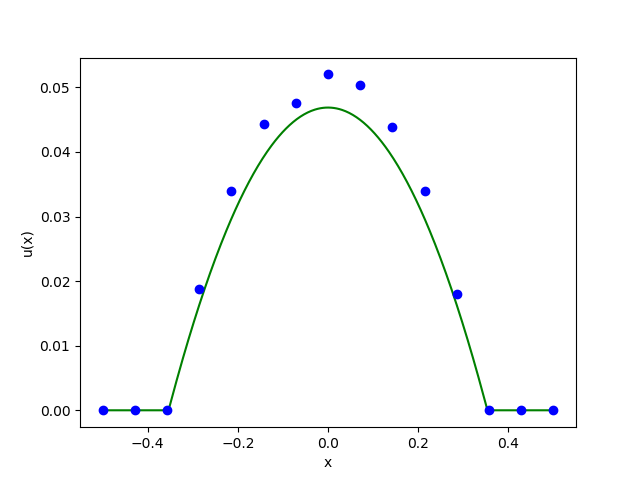
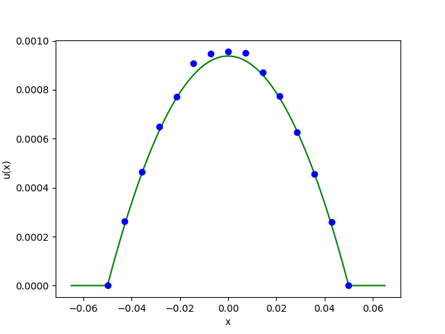
Figure 1: Approximate solution (blue) and reference solution (green) for the Poisson equation on the $\mathbb{R}^{2}$ (left) and on the $\mathbb{R}^{100}$ (right).

4.2 Quadratic gradient

The second example is a semilinear PDE with a quadratic gradient term.

Let $r\in(0,\infty)$, $G=\left\{x\in\mathbb{R}^{d}\colon|x|<r\right\}$, and $\partial G=\left\{x\in\mathbb{R}^{d}\colon|x|=r\right\}$. We consider the PDE

$$\Delta u(x)+|\nabla u(x)|^{2}=2e^{-u(x)}, \quad x\in G,$$ (15)

$$u(x)=\log\!\left(\frac{r^{2}+1}{d}\right), \quad x\in\partial G.$$

corresponding to the BSDE

$$dX_{t} =\sqrt{2}dW_{t},\qquad X_{0}=x,$$ (16)

$$f(x,y,\zeta) =|\zeta|^{2}-2e^{-y},\qquad\xi=\log\left(\frac{|r|^{2}+1}{d}\right).$$ (17)

In addition, this example we have an analytic reference solution given by

$$u(x) =\log\left(\frac{|x|^{2}+1}{d}\right).$$

4.2.1 Numerical results

As in the previous example we compute $u(x)$ for 15 different values of $x$ on the $\mathbb{R}^{2}$ and the $\mathbb{R}^{100}$. Figure 2 shows the approximate solution of $u$ obtained by the DNN algorithm on the diagonal points $\{(x,\dots,x)\in\mathbb{R}^{d}\colon x\in[-r,r]\}$ (in blue) and the analytical reference solution (in green). Table 2 contains the parameters we use.

$d$	$r$	$N$	$T$	E	M	validation size	time per eight points
2	1	100	5	500	64	256	204.58 s
100	1	100	0.1	500	64	256	321.13 s

Table 2: Parameters for the equation with quadratic gradient.

While classical numerical methods for PDEs would be a much better choice in the case $d=2$, their application would not be feasible in the case $d=100$.

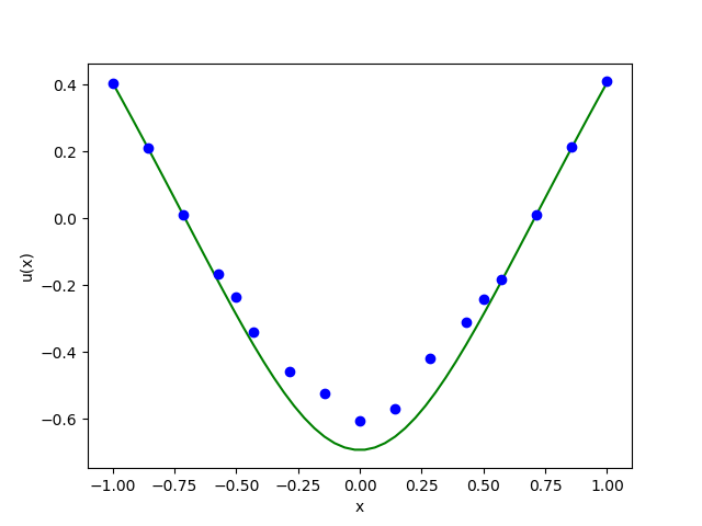
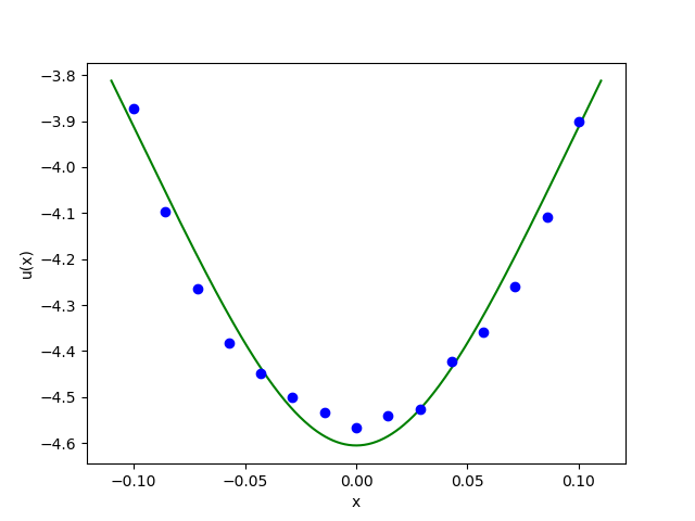
Figure 2: Approximate solution (blue) and reference solution (green) for the equation with quadratic gradient on the $\mathbb{R}^{2}$ (left) and on the $\mathbb{R}^{100}$ (right).

4.3 Dividend maximization

The goal of this paper was to show how to use the proposed DNN algorithm to solve high-dimensional control problems that arise in insurance mathematics. We finally arrived at the point where we are ready to do so.

Our example comes from [68], where the author studies De Finetti’s dividend maximization problem in a setup with incomplete information about the current state of the market. The hidden market-state process determines the trend of the surplus process of the insurance company and is modeled as a $d$-state Markov chain. Using stochastic filtering, in [68] they achieve to transform the one-dimensional problem under incomplete information to a $d$-dimensional problem under complete information. The cost is $(d-1)$ additional dimensions in the state space. We state the problem under complete information using different notation than in [68] in order to avoid ambiguities.

The probability that the Markov chain modeling the market-state is in state $i\in\{1,\dots,d-1\}$ is given by

$$\pi_{i}(t)=x_{i}+\int_{0}^{t}\left(q_{d,i}+\sum_{j=1}^{d-1}(q_{j,i}-q_{d,i})\pi_{j}(s)\right)\,ds+\int_{0}^{t}\pi_{i}(s)\frac{a_{i}-\nu_{s}}{\rho}\,dB_{s},$$ (18)

where

$$\nu_{t}=a_{d}+\sum_{j=1}^{d-1}(a_{j}-a_{d})\pi_{j}(t),$$ (19)

$x_{i}\in(0,1)$, $B$ is a one-dimensional Brownian motion, $a_{1},\dots,a_{d}\in\mathbb{R}$ are the values of the surplus trend in the respective market-states of the hidden Markov chain, and $(q_{i,j})_{i,j\in\{1,\dots,d\}}\in\mathbb{R}^{d\times d}$ denotes the intensity matrix of the chain.

Let $(\ell_{t})_{t\in[0,\infty)}$ be the dividend rate process. The surplus of the insurance company is given by

$$\widetilde{X}^{d}_{t}=x_{d}+\int_{0}^{t}(\nu_{s}-\ell_{s})\,ds+\rho B_{t},\quad t\in[0,\infty),$$ (20)

where $x_{d},\rho\in(0,\infty)$. For later use we define also the dividend free surplus

$$X^{d}_{t}=x_{d}+\int_{0}^{t}\nu_{s}\,ds+\rho B_{t},\quad t\in[0,\infty).$$ (21)

The processes (18) and (20) form the $d$-dimensional state process underlying the optimal control problem we aim to solve.

The goal of the insurance company is to determine its value by maximizing the discounted dividends payments until the time of ruin $\eta=\inf\{t\in(0,\infty]\colon\widetilde{X}^{d}_{t}<0\}$, that is it seeks to find

$$u(x_{1},\dots,x_{d})=\sup_{(\ell_{t})_{t\in[0,\infty)}\in A}\mathbb{E}_{x_{1},\dots,x_{d}}\!\left[\int_{0}^{\eta}e^{-\delta t}\ell_{t}\,dt\right],$$ (22)

where $\delta\in(0,\infty)$ is a discount rate, $A$ is the set of admissible controls, and $\mathbb{E}_{x_{1},\dots,x_{d}}[\cdot]$ denotes the expectation under the initial conditions $\pi_{i}(0)=x_{i}$ for $i\in\{1,\dots,d-1\}$ and $\widetilde{X}^{d}_{0}=x_{d}$. Admissible controls are $(\mathcal{F}^{X^{d}}_{t})_{t\geq 0}$-progressively measurable, $[0,K]$-valued for $K\in(0,\infty)$, and fulfill $\ell_{t}\equiv 0$ for $t>\eta$, cf. [68].

In order to tackle the problem, we solve the corresponding Hamilton-Jacobi-Bellmann (HJB) equation from [68],

$$(\mathcal{L}-\delta)u+\sup_{\ell\in[0,K]}(\ell(1-u_{x_{d}}))=0,$$ (23)

where $\mathcal{L}$ is the second order degenerate elliptic operator

$$\mathcal{L}u =a_{d}u_{x_{d}}+\sum_{i=1}^{d-1}\left((a_{i}-a_{d})x_{i}u_{x_{d}}+\left(q_{di}+\sum_{j=1}^{d-1}(q_{ji}-q_{di})x_{i}\right)u_{x_{i}}+x_{i}\left(a_{i}-\nu\right)u_{x_{d}x_{i}}\right.$$

$$+\left.\frac{1}{2}\sum_{j=1}^{d-1}\left(\left(x_{i}\frac{a_{i}-\nu}{\rho}\right)\left(x_{j}\frac{a_{j}-\nu}{\rho}\right)u_{x_{i}x_{j}}\right)\right)+\frac{1}{2}\rho^{2}u_{x_{d}x_{d}}.$$

The supremum in (23) is attained at

$$\ell=\begin{cases}K,&u_{x_{d}}\leq 1\\ 0,&u_{x_{d}}>1.\end{cases}$$

Plugging this into (23) we end up with a $d$-dimensional semilinear degenerate elliptic PDE:

$$(\mathcal{L}-\delta)u+K(1-u_{x_{d}})\mathbbm{1}_{\{u_{x_{d}}\leq 1\}}=0.$$ (24)

The boundary conditions in $x_{d}$ direction are given by

$$u(x_{1},\dots,x_{d})=\begin{cases}K/\delta,&x_{d}\to\infty\\ 0,&x_{d}=0.\end{cases}$$

No boundary conditions are required for the other variables, cf. [68].

In [68, Corollary 3.6] it is proven that the unique viscosity solution to (24) solves the optimal control problem (22). Hence, we can indeed solve the control problem by solving the HJB equation.

For the numerical approximation we cut off $x_{d}$ at $r\in(0,\infty)$. Hence, $G=\left\{x\in\mathbb{R}^{d}\colon 0<x_{d}<r\right\}$ and $\partial G=\left\{x\in\mathbb{R}^{d}\colon x_{d}\in\{0,r\}\right\}$.

For the convenience of the reader we derive the BSDE corresponding to (24). The forward equation is given by

$$dX_{t}=(d\pi_{1}(t),\dots,d\pi_{d-1}(t),dX^{d}_{t})^{\top},\qquad X_{0}=x,\\$$

that is

$$dX_{t}=\mu(X_{t})dt+\sigma(X_{t})dW_{t},\qquad X_{0}=x,\\$$

where $W=(B,W^{2},\dots,W^{d})^{\top}$, $x=(x_{1},\dots,x_{d})^{\top}$, and

$$\mu(x)=\left(q_{d,1}+\sum_{j=1}^{d-1}(q_{j,1}-q_{d,1})x_{j},\dots,q_{d,d-1}+\sum_{j=1}^{d-1}(q_{j,d-1}-q_{d,d-1})x_{d-1},a_{d}+\sum_{j=1}^{d-1}(a_{j}-a_{d})x_{j}\right)^{\top},$$

$$\sigma(x)=\left(\begin{array}[]{cccc}x_{1}\frac{a_{1}-a_{d}+\sum_{j=1}^{d-1}(a_{j}-a_{d})x_{j}}{\rho}&0&\dots&0\\ \dots&0&\dots&0\\ x_{d-1}\frac{a_{d-1}-a_{d}+\sum_{j=1}^{d-1}(a_{j}-a_{d})x_{j}}{\rho}&0&\dots&0\\ \rho&0&\dots&0\\ \end{array}\right).$$

We claim that the BSDE associated to (24) is given in forward form by

$$u(X_{t}) =u(x)-\int_{0}^{t}[K(1-u_{x_{d}}(X_{s}))\mathbbm{1}_{\{u_{x_{d}}(X_{s})\leq 1\}}-\delta u(X_{s})]dt$$ (25)

$$\quad+\int_{0}^{t}\nabla u(X_{s})\sigma(X_{s})dW_{s}.$$

Applying Itô’s formula to $u(X)$ yields

$$u(X_{t}) =u(x)+\int_{0}^{t}\mathcal{L}u(X_{s})dt+\int_{0}^{t}\nabla u(X_{s})\sigma(X_{s})dW_{s}.$$ (26)

Combining (25) and (26) gives

$$u(x)-\int_{0}^{t}[K(1-u_{x_{d}}(X_{s}))\mathbbm{1}_{\{u_{x_{d}}(X_{s})\leq 1\}}-\delta u(X_{s})]dt+\int_{0}^{t}\nabla u(X_{s})\sigma(X_{s})dW_{s}$$

$$\quad=u(x)+\int_{0}^{t}\mathcal{L}u(X_{s})dt+\int_{0}^{t}\nabla u(X_{s})\sigma(X_{s})dW_{s}.$$

Canceling terms verifies (in a heuristic manner) (24).

Hence, the corresponding BSDE has the parameters

$$f(x,y,\zeta) =K(1-\zeta_{d})\mathbbm{1}_{\{\zeta_{d}\leq 1\}}-\delta y$$ (27)

and

$$\xi=\begin{cases}K/\delta,&X^{d}_{\tau}=r,\\ 0,&X^{d}_{\tau}=0,\end{cases}$$

if $\tau<\infty$.

4.3.1 Numerical results

As for this example we have no analytic reference solution at hand, we use the solution from [68] for the case $d=2$, which was obtained by a finite difference method and policy iteration. Then we show that the DNN algorithm also provides an approximation in high dimensions in reasonable computation time.

As in the previous examples we compute $u(x)$ on the $\mathbb{R}^{2}$ and on the $\mathbb{R}^{100}$ for 15 different values of $x$. Figure 3 shows the approximate solution of the HJB equation and hence the value of the insurance company obtained by the DNN algorithm (in blue) and the reference solution from [68] (in green) for the case $d=2$. For $d=100$ we have no reference solution at hand. Figure 4 shows the loss for a fixed value of $x$ in the case $d=100$. Tables 3 and 4 contain the parameters we use.

$d$	$r$	$K$	$\delta$	$\rho$	$a_{i}$	$N$	$T$	E	M	validation size	time per eight points
2	5	1.8	0.5	1	$\left(2-\frac{i}{d}\right)$	100	5	500	64	256	317.42 s
100	5	1.8	0.5	1	$\left(2-\frac{i}{d}\right)$	100	5	500	64	256	613.15 s

Table 3: Parameters for the dividend problem.

case	$i=j$ even	$i=j$ odd	$i=j+1$ even	$i=j+1\geq 3$ odd	$i=1$, $j=d$	otherwise
$q_{i,j}$	$-0.5$	$-0.25$	$0.5$	0.25	0.25	0

Table 4: Intensity matrix values for the dividend problem.

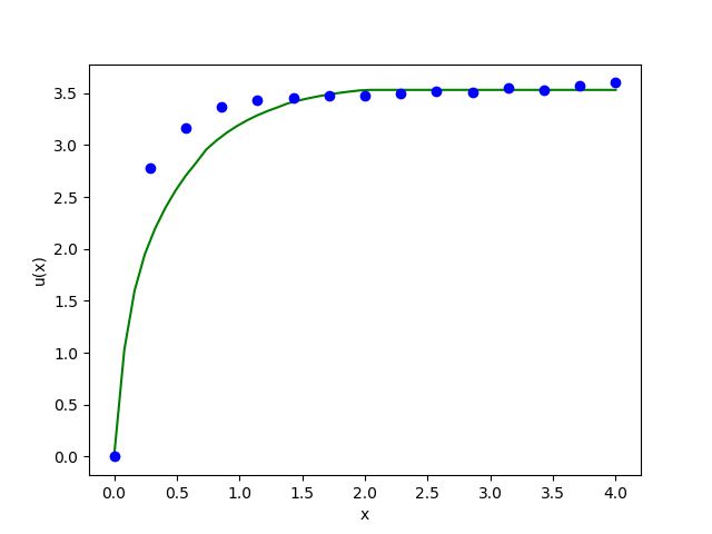
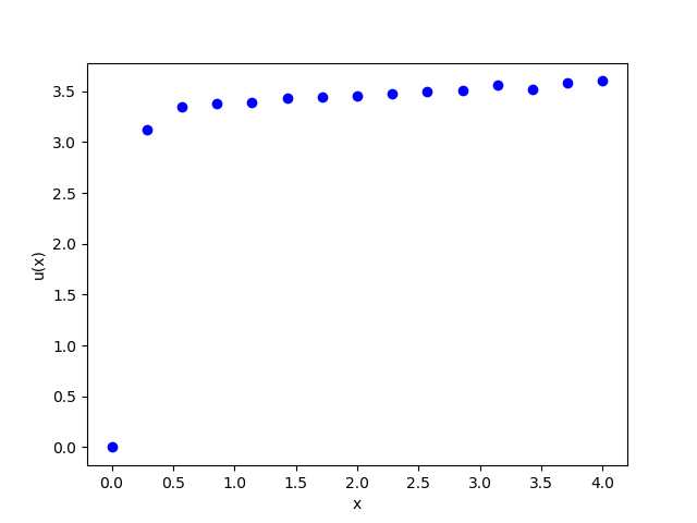
Figure 3: Approximate solution (blue) and reference solution (green) for the dividend problem on the $\mathbb{R}^{2}$ for fixed $\pi_{1}=\pi_{2}=0.5$ (left) and on the $\mathbb{R}^{100}$ for fixed $\pi_{1}=\dots=\pi_{100}=0.01$ (right, without reference solution).

Figure 4: Interpolated loss for the case $d=100$.

5 Conclusion

The goal of this paper was to compute the risk measure given by the expected discounted future dividend payments in a complex high-dimensional economic environment. This demonstrates the effectiveness of using DNN algorithms for solving some high-dimensional PDE problems in insurance mathematics that cannot be solved by classical methods. In the literature the focus so far was on parabolic PDE problems; however, in insurance mathematics we often face problems up to an unbounded random terminal time, e.g., the time of ruin of the insurance company, leading to (degenerate) elliptic problems.

Hence, we have proposed a novel deep neural network algorithm for a large class of semilinear (degenerate) elliptic PDEs associated to infinite time horizon control problems in high dimensions. The method extends the DNN algorithm proposed by Han, Jetzen, and E [33], which was developed for parabolic PDEs, to the case of (degenerate) elliptic semilinear PDEs. We have attacked the problem inspired by a series of results by Pardoux [55].

Of course, in low dimensions one would not use the proposed DNN algorithm – classical methods are more efficient. However, recent models are frequently high dimensional, in which case classical methods fail due to the curse of dimensionality. Then the DNN algorithm presented here can be applied to compute the desired quantity.

We emphasize that the method presented here can also be applied to many other high-dimensional semilinear (degenerate) elliptic PDE problems in insurance mathematics and beyond.

An implementation of the algorithm is provided on Github under a creative commons license.

References

- [1] H. Albrecher and S. Thonhauser. Optimality results for dividend problems in insurance. RACSAM Revista de la Real Academia de Ciencias Exactas, Fisicas y Naturales. Serie A. Matematicas, 103(2):295–320, 2009.
- [2] S. Asmussen and M. Taksar. Controlled diffusion models for optimal dividend pay-out. Insurance: Mathematics and Economics, 20(1):1–15, 1997.
- [3] B. Avanzi. Strategies for dividend distribution: A review. North American Actuarial Journal, 13(2):217–251, 2009.
- [4] P. Azcue and N. Mular. Stochastic Optimization in Insurance – A Dynamic Programming Approach. Springer Briefs in Quantitative Finance. Springer, New York, Heidelberg, Dordrecht, London, 2014.
- [5] C. Beck, S. Becker, P. Cheridito, A. Jentzen, and A. Neufeld. Deep splitting method for parabolic PDEs. arXiv:1907.03452, 2019.
- [6] C. Beck, S. Becker, P. Grohs, N. Jaafari, and A. Jentzen. Solving stochastic differential equations and Kolmogorov equations by means of deep learning. arXiv:1806.00421, 2018.
- [7] C. Beck, W. E, and A. Jentzen. Machine learning approximation algorithms for high-dimensional fully nonlinear partial differential equations and second-order backward stochastic differential equations. Journal of Nonlinear Science, 29(4):1563–1619, 2019.
- [8] C. Beck, L. Gonon, and A. Jentzen. Overcoming the curse of dimensionality in the numerical approximation of high-dimensional semilinear elliptic partial differential equations. arXiv:2003.00596, 2020.
- [9] C. Beck, F. Hornung, M. Hutzenthaler, A. Jentzen, and T. Kruse. Overcoming the curse of dimensionality in the numerical approximation of Allen-Cahn partial differential equations via truncated full-history recursive multilevel Picard approximations. arXiv:1907.06729, 2019.
- [10] S. Becker, P. Cheridito, and A. Jentzen. Deep optimal stopping. Journal of Machine Learning Research, 20:74, 2019.
- [11] S. Becker, P. Cheridito, A. Jentzen, and T. Welti. Solving high-dimensional optimal stopping problems using deep learning. arXiv:1908.01602, 2019.
- [12] J. Berg and K. Nyström. A unified deep artificial neural network approach to partial differential equations in complex geometries. Neurocomputing, 317:28–41, 2018.
- [13] J. Berner, P. Grohs, and A. Jentzen. Analysis of the generalization error: Empirical risk minimization over deep artificial neural networks overcomes the curse of dimensionality in the numerical approximation of Black–Scholes partial differential equations. SIAM Journal on Mathematics of Data Science, 2(3):631–657, 2020.
- [14] P. Briand, B. Delyon, Y. Hu, É. Pardoux, and L. Stoica. solutions of backward stochastic differential equations. Stochastic Processes and their Applications, 108(1):109–129, 2003.
- [15] P. Briand and Y. Hu. Stability of BSDEs with random terminal time and homogenization of semi-linear elliptic PDEs. Journal of Functional Analysis, 155(2):455–494, 1998.
- [16] Q. Chan-Wai-Nam, J. Mikael, and X. Warin. Machine learning for semi linear PDEs. Journal of Scientific Computing, 79(3):1667–1712, 2019.
- [17] Y. Chen and J. W. Wan. Deep neural network framework based on backward stochastic differential equations for pricing and hedging american options in high dimensions. Quantitative Finance, pages 1–23, 2020.
- [18] F. Confortola and P. Briand. Quadratic BSDEs with random terminal time and elliptic PDEs in infinite dimension. Electronic Journal of Probability, 13:1529–1561, 2008.
- [19] R. Darling and É. Pardoux. Backwards SDE with random terminal time and applications to semilinear elliptic PDE. The Annals of Probability, 25(3):1135–1159, 1997.
- [20] B. de Finetti. Su un’impostazione alternativa della teoria collettiva del rischio. Transactions of the XVth International Congress of Actuaries, 2:433–443, 1957.
- [21] T. Dockhorn. A discussion on solving partial differential equations using neural networks. arXiv:1904.07200, 2019.
- [22] W. E, J. Han, and A. Jentzen. Deep learning-based numerical methods for high-dimensional parabolic partial differential equations and backward stochastic differential equations. Communications in Mathematics and Statistics, 5(4):349–380, 2017.
- [23] W. E and B. Yu. The deep Ritz method: A deep learning-based numerical algorithm for solving variational problems. Commun. Math. Stat., 6:1–12, 2018.
- [24] D. Elbrächter, P. Grohs, A. Jentzen, and C. Schwab. DNN expression rate analysis of high-dimensional PDEs: application to option pricing. arXiv:1809.07669, 2018.
- [25] A.-M. Farahmand, S. Nabi, and D. Nikovski. Deep reinforcement learning for partial differential equation control. 2017 American Control Conference (ACC), pages 3120–3127, 2017.
- [26] M. Fujii, A. Takahashi, and M. Takahashi. Asymptotic expansion as prior knowledge in deep learning method for high dimensional BSDEs. Asia-Pacific Financial Markets, 26(3):391–408, 2019.
- [27] L. Gonon, P. Grohs, A. Jentzen, D. Kofler, and D. Šiška. Uniform error estimates for artificial neural network approximations. arXiv:1911.09647, 2019.
- [28] L. Goudenège, A. Molent, and A. Zanette. Machine learning for pricing American options in high dimension. arXiv:1903.11275, 2019.
- [29] P. Grohs and L. Herrmann. Deep neural network approximation for high-dimensional elliptic PDEs with boundary conditions. arXiv:2007.05384, 2020.
- [30] P. Grohs, F. Hornung, A. Jentzen, and P. von Wurstemberger. A proof that artificial neural networks overcome the curse of dimensionality in the numerical approximation of Black-Scholes partial differential equations. arXiv:1809.02362, 2018.
- [31] P. Grohs, F. Hornung, A. Jentzen, and P. Zimmermann. Space-time error estimates for deep neural network approximations for differential equations. arXiv:1908.03833, 2019.
- [32] P. Grohs, A. Jentzen, and D. Salimova. Deep neural network approximations for Monte Carlo algorithms. arXiv:1908.10828, 2019.
- [33] J. Han, A. Jentzen, and W. E. Solving high-dimensional partial differential equations using deep learning. Proceedings of the National Academy of Sciences, 115(34):8505–8510, 2018.
- [34] J. Han and J. Long. Convergence of the deep BSDE method for coupled FBSDEs. Probability, Uncertainty and Quantitative Risk, 5(1):1–33, 2020.
- [35] J. Han, M. Nica, and A. R. Stinchcombe. A derivative-free method for solving elliptic partial differential equations with deep neural networks. ”Journal of Computational Physics, 419:109672, 2020.
- [36] P. Henry-Labordère. Deep primal-dual algorithm for BSDEs: Applications of machine learning to CVA and IM. Available at SSRN 3071506, 2017.
- [37] K. Hornik. Approximation capabilities of multilayer feedforward networks. Neural networks, 4(2):251–257, 1991.
- [38] K. Hornik, M. Stinchcombe, and H. White. Multilayer feedforward networks are universal approximators. Neural networks, 2(5):359–366, 1989.
- [39] C. Huré, H. Pham, and X. Warin. Some machine learning schemes for high-dimensional nonlinear PDEs. arXiv:1902.01599, 2019.
- [40] M. Hutzenthaler, A. Jentzen, T. Kruse, T. A. Nguyen, and P. von Wurstemberger. Overcoming the curse of dimensionality in the numerical approximation of semilinear parabolic partial differential equations. arXiv:1807.01212, 2018.
- [41] M. Hutzenthaler, A. Jentzen, and P. von Wurstemberger. Overcoming the curse of dimensionality in the approximative pricing of financial derivatives with default risks. Electronic Journal of Probability, 25:73 pp, 2020.
- [42] Martin Hutzenthaler, Arnulf Jentzen, Thomas Kruse, and Tuan Anh Nguyen. A proof that rectified deep neural networks overcome the curse of dimensionality in the numerical approximation of semilinear heat equations. SN Partial Differential Equations and Applications, 1:1–34, 2020.
- [43] A. Jacquier and M. Oumgari. Deep PPDEs for rough local stochastic volatility. arXiv:1906.02551, 2019.
- [44] M. Jeanblanc-Piqué and A. N. Shiryaev. Optimization of the flow of dividends. Russian Mathematical Surveys, 50(2):257–277, 1995.
- [45] A. Jentzen, D. Salimova, and T. Welti. A proof that deep artificial neural networks overcome the curse of dimensionality in the numerical approximation of Kolmogorov partial differential equations with constant diffusion and nonlinear drift coefficients. arXiv:1809.07321, 2018.
- [46] Z. Jiang and M. Pistorius. Optimal dividend distribution under markov regime switching. Finance and Stochastics, 16(3):449–476, 2012.
- [47] P. Kritzer, G. Leobacher, M. Szölgyenyi, and S. Thonhauser. Approximation methods for piecewise deterministic markov processes and their costs. Scandinavian Actuarial Journal, 2019(4):308–335, 2019.
- [48] G. Kutyniok, P. Petersen, M. Raslan, and R. Schneider. A theoretical analysis of deep neural networks and parametric PDEs. arXiv:1904.00377, 2019.
- [49] G. Leobacher, M. Szölgyenyi, and S. Thonhauser. Bayesian dividend optimization and finite time ruin probabilities. Stochastic Models, 30(2):216–249, 2014.
- [50] Z. Long, Y. Lu, X. Ma, and B. Dong. PDE-Net: Learning PDEs from Data. In Proceedings of the 35th International Conference on Machine Learning, pages 3208–3216, 2018.
- [51] L. Lu, X. Meng, Z. Mao, and G. E. Karniadakis. DeepXDE: A deep learning library for solving differential equations. arXiv:1907.04502, 2019.
- [52] K. O. Lye, S. Mishra, and D. Ray. Deep learning observables in computational fluid dynamics. Journal of Computational Physics, 410:109339, 2020.
- [53] M. Magill, F. Qureshi, and H. de Haan. Neural networks trained to solve differential equations learn general representations. Advances in Neural Information Processing Systems, pages 4071–4081, 2018.
- [54] B. Øksendal. Stochastic differential equations. Springer, 2003.
- [55] É. Pardoux. Backward stochastic differential equations and viscosity solutions of systems of semilinear parabolic and elliptic PDEs of second order. In Stochastic Analysis and Related Topics VI, pages 79–127. Springer, 1998.
- [56] É. Pardoux. BSDEs, weak convergence and homogenization of semilinear PDEs. In Nonlinear analysis, differential equations and control, pages 503–549. Springer, 1999.
- [57] H. Pham and X. Warin. Neural networks-based backward scheme for fully nonlinear PDEs. arXiv:1908.00412, 2019.
- [58] R. Radner and L. Shepp. Risk vs. profit potential: A model for corporate strategy. Journal of Economic Dynamics and Control, 20(8):1373–1393, 1996.
- [59] M. Raissi. Deep hidden physics models: Deep learning of nonlinear partial differential equations. J. Mach. Learn. Res., 19(1):932–955, 2018.
- [60] C. Reisinger and Y. Zhang. Rectified deep neural networks overcome the curse of dimensionality for nonsmooth value functions in zero-sum games of nonlinear stiff systems. arXiv:1903.06652, 2019.
- [61] A. M. Reppen, J.-C. Rochet, and H. M. Soner. Optimal dividend policies with random profitability. Mathematical Finance, 30(1):228–259, 2020.
- [62] M. Royer. BSDEs with a random terminal time driven by a monotone generator and their links with PDEs. Stochastics and stochastic reports, 76(4):281–307, 2004.
- [63] H. Schmidli. Stochastic Control in Insurance. Probability and its Applications. Springer, London, 2008.
- [64] S. E. Shreve, J. P. Lehoczky, and D. P. Gaver. Optimal consumption for general diffusions with absorbing and reflecting barriers. SIAM Journal on Control and Optimization, 22(1):55–75, 1984.
- [65] J. Sirignano and K. Spiliopoulos. DGM: A deep learning algorithm for solving partial differential equations. Journal of computational physics, 375:1339–1364, 2018.
- [66] L. Sotomayor and A. Cadenillas. Classical and singular stochastic control for the optimal dividend policy when there is regime switching. Insurance: Mathematics and Economics, 48:344–354, 2011.
- [67] M. Szölgyenyi. Bayesian dividend maximization: A jump diffusion model. In M. Vanmaele, G. Deelstra, A. De Schepper, J. Dhaene, W. Schoutens, S. Vanduffel, and D. Vyncke, editors, Handelingen Contactforum Actuarial and Financial Mathematics Conference, Interplay between Finance and Insurance, February 7-8, 2013, pages 77–82. Koninklijke Vlaamse Academie van België voor Wetenschappen en Kunsten, Brussel, 2013.
- [68] M. Szölgyenyi. Dividend maximization in a hidden Markov switching model. Statistics & Risk Modeling, 32(3-4):143–158, 2016.
- [69] J. Zhu and F. Chen. Dividend optimization for regime-switching general diffusions. Insurance: Mathematics and Economics, 53:439–456, 2013.