A colloquium on the variational method applied to excitons in 2D materials

Abstract

In this colloquium, we review the research on excitons in van der Waals heterostructures from the point of view of variational calculations. We first make a presentation of the current and past literature, followed by a discussion on the connections between experimental and theoretical results. In particular, we focus our review of the literature on the absorption spectrum and polarizability, as well as the Stark shift and the dissociation rate. Afterwards, we begin the discussion of the use of variational methods in the study of excitons. We initially model the electron-hole interaction as a soft-Coulomb potential, which can be used to describe interlayer excitons. Using an ansatz, based on the solution for the two-dimensional quantum harmonic oscillator, we study the Rytova-Keldysh potential, which is appropriate to describe intralayer excitons in two-dimensional (2D) materials. These variational energies are then recalculated with a different ansatz, based on the exact wavefunction of the 2D hydrogen atom, and the obtained energy curves are compared. Afterwards, we discuss the Wannier-Mott exciton model, reviewing it briefly before focusing on an application of this model to obtain both the exciton absorption spectrum and the binding energies for certain values of the physical parameters of the materials. Finally, we briefly discuss an approximation of the electron-hole interaction in interlayer excitons as an harmonic potential and the comparison of the obtained results with the existing values from both first–principles calculations and experimental measurements.

1 Introduction

Alongside graphene, a wide range of bi-dimensional materials are currently studied and have a plethora of different physical properties and applicationsMounet_2018 . An important subclass of these materials is the family of transition-metal dichalcogenides with chemical formula $\mathrm{MX_{2}}$, where $\mathrm{M}$ is a transition metal and $\mathrm{X}$ a chalcogen atom. These materials, specifically those with group-VI transition metals, are semiconductors which exhibit strong light-matter coupling, as well as having direct band gaps in the infrared and visible spectral regimes. Having been studied in their bulk form since the 1960’s1963 ; Fortin_1982 , the advent of the study of two-dimensional (2D) layers with atomic scale thickness renewed the interest in these materials and their properties that make them good candidates for various applications in optics and optoelectronicsmueller_exciton_2018 .

The optical response of these semiconductors is mainly dominated by the excitation of electrons from the valence band to the conduction bandRevModPhys.90.021001 ; nwu078 . Such a phenomena can be described by a pair of interacting (effective) particles, one being a conduction electron and the other being a hole left in the valence band, with opposite charge to the electron (Figure 1–a). Considering frequencies above the band gap, a transition from the valence to the conduction band is possible, which means that the absorption becomes finite. For certain materials, absorption peaks can be measured below the band gap, which can be explained by the presence of excitonic states (bound states of the said electron and hole).

As the electron and hole are of opposite charges, the most natural formulation of their interaction will be an attractive interaction. This will lead to the possibility of the formation of bound states between these particles, analogous to those formed between an electron and a proton in the hydrogen atomKnox_1983 . Unfortunately, the small effective mass of the particles in question and large screening effects means that the excitonic binding energy in bulk materials is of the order of $\mathrm{meV}$, while the room-temperature thermal fluctuations are about $25\,\mathrm{meV}$. These fluctuations mask excitonic effects unless the material is sufficiently cooled down.

The hydrogen atom and, consequently, hydrogen-like problems are some of the most studied systems in physics. While the simplest model consisting only of the Coulomb interaction has a well known exact solution, when one wishes to introduce more complex interactions no exact solutions are known. This becomes increasing problematic when one wishes to study systems with local/non-local screening, or finite (and externally fixed) minimum separation between particles.

In 2D transition-metal dichalcogenides (TMDs), where the screening effect is reduced relatively to their bulk counterparts, the exciton binding energies reach values the order of $100\,\mathrm{meV}$. Therefore, these class of excitons are more easily accessible to experimental study, as they are observable at room temperature. As an example, $\mathrm{WSe}_{2}$ in a fused quartz substrate presents two excitonic peaks in the linear absorption at $1.65$ and $2.08\,\mathrm{eV}$. The presence of two peaks instead of a single one is the signature of strong spin-orbit coupling in this system. The position of these peaks in frequency, however, was not consistent with the bare Coulomb interaction, which shows the necessity of including screening effects in the electron-hole interaction.

The simplest way of including a screening-like effect is via the soft-Coulomb potential, which introduces a material-dependent minimum separation-like parameter between the electron and the hole. Although this approach might seem somewhat artificial, it is relevant to the discussion of interlayer excitons (see below). Another of these potentials is the Rytova-Keldysh potentialrytova1967 ; 1979JETPL..29..658K , which includes a material dependent parameter and reduces to the Coulomb potential in the regime when this parameter is zero. Mathematically, this potential is significantly more complex than the Coulomb potential, which in turn further complicates the analytical work in determining the absorption spectrum. It can, however, be closely approximated by simpler functions, which might help with the calculations for the absorption spectrum.

Another relevant system is that of spatially separated excitons (also called indirect excitons, although this terminology may be misleading), where each element of the electron-hole pair is situated in a different layer, creating a minimum distance between the electron and the hole (Figure 1–b). These excitons are specially relevant in van der Waals (vdW) heterostructures, where multiple layers of different TMDs are stackedGeim_2013 ; Dong_2019 . With the previously-mentioned soft-Coulomb potential, this bias distance is easily introduced as a minimum separation parameter, which depends on the specific heterostructure. The obtained theoretical results (from either variational or numerical methods) can be compared with experimental results, where the minimum separation is usually of the order of the effective Bohr radius for an electron-hole pair in the material in question.

Figure 1: (a) Intralayer excitons in a TMD; (b) Interlayer excitons in two different TMDs.

Besides vdW heterostructures, where the screening effects reflect the nature of the different materials in each layer, these same screening effects are fundamental when one wishes to study TMD monolayers surrounded by a dielectric medium with a dielectric constant different from that of the TMDThygesen_2017 . In these systems, as mentioned before, the physics of the electron-hole is better modeled by replacing the Coulomb potential with the Rytova-Keldysh potential rytova1967 ; 1979JETPL..29..658K with parameters related to the relative dielectric constants of the media surrounding the monolayer, as well as the 2D polarizability of the TMD brunetti_optical_2018 ; van_tuan_coulomb_2018 ; zhang_two-dimensional_2019 ; Scharf_2019 ; kamban_interlayer_2020 ; Cavalcante_2018 .

2 Brief Historical Review

After the first mechanical exfoliation of graphene in 2004 by Novoselov and Geimnovoselov_electric_2004 , the field of two-dimensional materials boomed. Just one year after the exfoliation of graphene, in 2005, Novoselov et al.novoselov_two-dimensional_2005 showed that the same technique could be applied to isolate other monolayer materials. This was specifically done for a 2D semiconductor, molybdenum disulfide ($\mathrm{MoS_{2}}$). Despite these advances, most of the research on 2D materials was focused on the unknown properties of graphene. This changed somewhat in 2010, when Heinz and Wang demonstrated Mak2010 ; wang_2010 (independently) that a $\mathrm{MoS_{2}}$ monolayer exhibits strong photoluminescence emission and has a direct band gap. The bandgaps in the near-infrared to visible range, the high photo-catalytic and mechanic stability, the decent charge carrier mobility, and the presence of exotic many-body phenomena make these materials extremely interesting from a fundamental research, device application, and innovation perspectivesWurstbauer_2017 . Despite the quick recognition that the optical response of transition metal dichalcogenides arises from excitons, quantitative measurements of the binding energy were only reported around 2014 chernikov_2014 . Excitons in these materials are tightly bound, and dominate the optical response even at room-temperature Mak_2012 ; He_2014 . This possibility comes about due to the reduced screening among the electrons in the TMDs, which has its origin in the low dimensionality of the 2D materials.

The demonstration of valley-selective optical excitation, in 2012, brought forth the field of TMD-based valleytronics Xiao_2012 . In 2013 Geim2013 , the advent of vdW heterostructures allowed the fabrication of TMD heterostructures, and consequently the observation of interlayer excitons. The more recent developments of optoelectronic devices, whose structure resembles that of the first $\mathrm{MoS_{2}}$ monolayer field-effect transistor (demonstrated in 2011 by Kis et alkis_2011 ) has happened in parallel with the research on the optical properties of TMDs. This same structure was used to realized atomically thin phototransistors one year later Yin_2011 .

The realization of atomically thin p-n junctions for both vertical Pospischil_2014 and lateral Furchi2014 geometries, in 2014, lead to the realization of light-emitting diodes, solar cells, and photodiodes. The potential efficiency of these devices was greatly improved by the 2015 demonstration of near-unity photon quantum yield in a TMD monolayer Amani_2015 . More recently, in 2017, the role of dark exciton states has become a major field of research, with optically allowed and forbidden dark excitons forming due to weak dielectric screening and strong geometrical confinement in TMD-based vdW heterostructures Zhang_2017 ; Molas_2017 .

Recently, the calculation and the experimental measurements of the Stark-shift and ionization rate of excitons in TMD has attracted considerable attention scharf_excitonic_2016 ; haastrup_stark_2016 ; massicotte_dissociation_2018 ; Rigosi_2015 . The possibility of increasing the efficiency of photodetectors using the Stark effect has grown the interest in this topic. However, the same class of problems is largely understudied in vdW heterostructures, with only one paper published so far on this topic kamban_interlayer_2020 .

The interest in the optical and excitonic properties of atomically thin TMDs Berkelbach_2018 has peaked in recent years, with numerous works focused on the study of both the excitonic binding energies aquino_accurate_2005 ; scharf_excitonic_2016 ; grasselli_variational_2017 ; inarrea_effects_2019 , exciton-exciton/exciton-electron interactions Shahnazaryan_2017 , strain effects Aas_2018 , their presence in vdW twisted heterostructures Jin_2019 , anisotropic semiconductors Castellanos_Gomez_2015 and quantum dots Li_2015 ; Pawbake_2016 ; Choi_2017 ; Ratnikov_2020 , and several magneto-optical effects chaves_excitonic_2017 ; have_excitonic_2019 ; henriques_excitonic_2020 ; henriques_optical_2020 published by many.

In what follows, we will briefly review some of the various approaches used in the study of excitons in vdW heterostructures, starting from the study of the electron-hole interaction in both monolayer TMDs van_tuan_coulomb_2018 ; durnev_excitons_nodate and vdW heterostructures van_der_donck_excitons_2018 ; brunetti_optical_2018 ; Castellanos_Gomez_2014 , as well as the study of screening effects in the interaction among the charge carriers Zhang_2019 ; Scharf_2019 .

3 Connection with Experimental Results

Discovered in 1913 by StarkStark_1914 , the Stark effect consists in the splitting of the spectral lines due to the presence of an external static electric field (analogously to the Zeeman effect). This effect is greatly enhanced by excitons in vdW heterostructures, as the electron and the hole that form the exciton are “pulled” in opposing directions by the external field, but remain confined in the material until the field is strong enough to dissociate it.

For weak electric fields, the Stark shifts of electrons vary, in accordance with perturbation theory, approximately quadratically with the external field $\mathcal{E}$, i.e., $E\approx E_{0}-\frac{1}{2}\alpha\mathcal{E}^{2}$, where $E_{0}$ is the unperturbed energy and $\alpha$ the in-plane polarizability. This allows for the calculation of the polarizability, which can then be used as a comparison against experimental results. The calculation of the polarizabilities reveals that they are significantly larger (around $3\times$ greater) for interlayer excitons, compared to their monolayer counterparts kamban_interlayer_2020 . This phenomena in bilayer vdW heterostructures can be explained by the increased screening and the vertical separation of the electron-hole pair, both of which reduce the binding energy and, therefore, facilitate the polarization of the exciton.

As the electron and the hole are pulled in opposing directions by the external field, the exciton may dissociate. This dissociation is realized by a non-vanishing imaginary part of the energy eigenvalue. Knowing the imaginary part of the energy eigenvalue, one can quickly calculate the field dissociation rate as $\Gamma=-2\,\mathrm{Im}E/\hbar$. Kamban and Pedersenkamban_interlayer_2020 obtain this imaginary part by applying the external complex scaling method Simon_1979 ; McCurdy_1991 , i.e., by rotating the radial coordinate into the complex plane by an angle $\phi$ outside of a specific radius $R$. The equation for the eigenstate is then split into the radial and the angular parts. The former is dealt with using a finite element basis consisting of Legendre polynomials, while the latter is solved using a cosine basis.

The dissociation times can be approximated as $\tau=1/\Gamma$ and are, at least, $10$ orders of magnitude greater than the experimentally obtained $50\,\mathrm{fs}$ required for holes to tunnel into the $\mathrm{WS_{2}}$ layer of a $\mathrm{MoS_{2}}/\mathrm{WS_{2}}$ heterostructure Hong_2014 . This time will likely be affected by material– (and medium) specific parameters, as these influence both the band gap and the binding energies of the excitons Meckbach_2018 ; Kumar_2018 . This large discrepancy is explained by the transition from intralayer to interlayer excitons (due to the staggered/type-II band alignment, see Fig. 2) before the field can dissociate these same excitons. Also, the luminescence exhibited by these interlayer excitons is exhibited at energies lower than that for intralayer complexes Vialla_2019 , as is clear from the band diagram of Fig. 2.

Figure 2: Mechanism for interlayer exciton formation: (i) A photon of energy $\hbar\omega_{0}$ is absorbed in MoSe₂ creating a intralayer exciton; (ii) the hole thus tunnels to the valence band of the nearby WSe₂; (iii) due to phonon absorption the hole moves to the top of the valence band of WSe₂; (iv) the strong electrostatic interaction between the electron and hole in the two different layers forms an intralayer exciton. (This image is adapted from Ref. Malic-2019 .)

After tunneling, interlayer excitons have long lifetime due to the small overlap of the individual electron and hole wave functions Miller_2017 . As such, when an in-plane field is applied, intralayer excitons will tunnel into interlayer excitons with sufficiently long lifetimes for them to dissociate. The much larger dissociation rates of interlayer excitons when compared to intralayer ones corroborates this, with $\Gamma\sim 10^{4}\,\mathrm{s}^{-1}$ for interlayer excitons in a freely suspended (i.e., not surrounded by a dielectric medium) $\mathrm{MoS_{2}}/\mathrm{WS_{2}}$ heterostructure, but only $\Gamma\sim 10^{-38}\,\mathrm{s}^{-1}$ for monolayer $\mathrm{MoS_{2}}$ (at $\mathcal{E}=10\,\mathrm{V}/\mu\mathrm{m}$)Kamban_2019 .

Furthermore, for the same electric field intensity, the dissociation rates for intralayer excitons in the top and bottom layers of $\mathrm{MoS_{2}}/\mathrm{WS_{2}}$ structures differ by seven orders of magnitude ($\Gamma\sim 2.1\times 10^{-3}\,\mathrm{s}^{-1}$ and $\Gamma\sim 2.9\times 10^{4}\,\mathrm{s}^{-1}$, respectively), which can be explained from the reduced masses in each material $\mu\approx 0.25,\,0.15$ (in units of the bare electron mass), respectively.

When studying exciton dissociation it is also important to take into account their radiative lifetimes. Wang et al.Wang_2016 focus their efforts on $\mathrm{Mo}\mathrm{S}_{2}$, calculating a radiative lifetime of around $180-300\,\mathrm{fs}$, in good agreement with recent experimental results for excitons with near-zero momentum in $\mathrm{WSe_{2}}$, in the range $150-250\,\mathrm{fs}$ Moody_2015 . Furthermore, Wang et al.Wang_2016 show that excitons with very long $\left(\geq 1\,\mathrm{ns}\right)$ exciton lifetimes that have been observed in clean $\mathrm{MoS_{2}}$ monolayers at small photoexcited exciton densities Amani_2015 are consistent with strongly localized excitons.

The absorption spectrum is one of the most used physical quantity of comparison between theoretical calculations and experimental results regarding both excitons Han_2018 and trions Courtade_2017 . These theoretical calculations come from both analytical, quasi-analytical and numerical approaches, usually expressed in terms of the optical conductivity. Looking specifically at some recent works regarding the calculation of the absorption spectrum, we mention Zhang et al.zhang_absorption_2014 , Van der Donck and Peetersvan_der_donck_excitons_2017 ; van_der_donck_interlayer_2018 , and Henriques et al.henriques_optical_2020 . Recent numerical studies van_der_donck_excitons_2017 also focus on the importance of considering a multiband model (including spin-orbit coupling) when calculating the exciton/trion binding energies and their absorption spectrum (a trion is a charged complex, which in a $n$-doped semiconductor is composed of the two electrons and a hole).

There are two complementary methods of accessing the optical properties of 2D materials: photoluminescence (PL) and absorption measurements ($\Delta R/R$). They both convey similar information. Ruppert et al. Ruppert-2014 measured the PL and the absorption in MoTe₂ multilayers down to the single layer case. They showed that the PL signal increases significantly when one moves from the bulk crystal to the single layer limit (see Fig. 3). This led these authors to conclude that MoTe₂ single layer is a direct band gap material with a band-gap of 1.1 eV, thus extending the class of 2D direct band gap materials from the visible to the near-infrared.

Figure 3: Photoluminescence (PL) and absorbance spectra. (Left) PL spectrum for MoTe₂ multilayers. (Right) PL spectrum (black) and absorbance (orange) for MoTe₂ single layer. The strong PL signal for MoTe₂ single layer is evident. (Figure adapted from Ref. Ruppert-2014 .)

4 Variational Methods

One of the simplest approach to study systems for which there is no analytical solution is using variational methods, which allows one to obtain approximations to both the wavefunction and its corresponding energy eigenvalue. The obtained closed-form analytical solutions give greater physical intuition on the result than numerical solutions. From the numerous works by multiple authors that employ variational methods, we specifically mention those by Grasselligrasselli_variational_2017 , Zhang et al.zhang_absorption_2014 ; zhang_two-dimensional_2019 , SeminaSemina_2019 , Planellesplanelles_simple_2017 , and Lundt et al.Lundt_2018 .

This method is usually performed in one of three ways: by choosing a trial wavefunction (ansatz) depending on a series of parameters and minimizing the expectation value of the Hamiltonian regarding these same parameters, quantum Monte Carlo methods Vialla_2019 , or by imposing a set of boundary conditions and constructing the wavefunction as a series expansion which obeys these same conditions by definition (frequently used when dealing with polygonal enclosures bhat_flexural_1987 ; liew_set_1991 ; Quintela_2020 ). This third procedure is not as usefull when one is dealing with infinite/semi–infinite regions, and will therefore remain undiscussed.

Over the next two sections, we will briefly describe two distinct approaches to variational methods, both based around choosing a trial function to solve an eigenvalue problem where the exact solution is either unknown or non–existent. Firstly, we will analyze the process described by Grasselligrasselli_variational_2017 , applying it afterwards to both a different potential and a different ansatz. Secondly, we discuss a work by Zhang et al.zhang_absorption_2014 , quickly reviewing the excitonic states, as well as the optical conductivity and the absorption spectum, and finally comparing the exciton radii and binding energies to those from first–principles approaches available in the literature (see Sec. 6.3).

5 The Variational Approach to 2D systems

The use of variational wave functions for describing excitonic properties has a long story in condensed matter and has been used in many systems, including quantum-well wires Brown_1987 . These same variational approaches have also been considered when it comes to the description of the excitonic Stark effect in confined systems Feng_1993 . These methods have also been applied to the study of biexcitons, quasi-particles consisting of two electrons and two holes Akimoto_1972 .

A simple example of variational methods is employed by Grasselligrasselli_variational_2017 to obtain the variational energies of the soft-Coulomb potential. Unlike the hydrogenic problem with the regular Coulomb interaction, exact solutions of the Schrödinger equation are not known for the soft-Coulomb potential. This potential is given by

$$V_{\mathrm{s-C}}\left(r\right)=-\frac{k}{\sqrt{r^{2}+d^{2}}},$$ (1)

where $k=e^{2}/\left(4\pi\epsilon_{0}\epsilon_{r}\right)$, $e$ is the electron charge, $\epsilon_{0}$ is the vacuum permittivity, and $\epsilon_{r}$ is the relative dielectric permittivity of the material, and is obtained for the bare Coulomb potential by introducing a fixed bias distance in the form of the parameter $d$. This potential is frequently used in semiconductor physics, as it:

1. overcomes the divergence issues of the Coulomb potential at the origin $\left(r=0\right)$, as well as the infinite binding energy of the ground-state in one-dimension Loudon_1959 . In this case, $d\neq 0$ is taken as a fixed cut-off parameter of the order of the screening length;

2. represents the coupling of an electron confined in a layer to a hole sitting in a different layer, a distance $d$ apart.

The method introduced by Grasselli will be presented in the context of a simple 2D material in Sec. 5.1, following which we will apply the same methodology for the more difficult Rytova-Keldysh potential in Sec. 5.2.

5.1 Interlayer Excitons in $\mathrm{hBN}$: the Soft–Coulomb Potential

Few layers hexagonal Boron Nitride (hBN) hosts excitons in the ultraviolet. If the number of layers is small we can treat this system as coupled 2D layers. In this case the parameter $d$ is the distance between the layers where the electron and the hole are respectively located (interlayer excitons). The problem of excitons in a single layer of hBN was treated by Henriques et al Henriques_2019 .

Considering a two-dimensional system, the ansätze for the ground- and first-excited states are based on the solutions for the quantum harmonic oscillator and are given bygrasselli_variational_2017

$$\phi_{0}\left(r\right) =\sqrt{\frac{\beta_{0}}{\pi}}e^{-\beta_{0}r^{2}/2},$$ (2)

$$\phi_{1x}\left(r,\theta\right) =\sqrt{\frac{\beta_{1}}{\pi}}\sqrt{2\beta_{1}}r\cos\theta e^{-\beta_{1}r^{2}/2},$$ (3)

where $\beta_{0}$ and $\beta_{1}$ are variational parameters. The $y$–component for the first-excited state is, by symmetry, degenerate and mutually orthogonal with the $x$–component and, as such, will not be discussed.

The expectation values of the Hamiltonian

$$H\left(r\right)=-\frac{\hbar^{2}}{2m}\nabla^{2}+V\left(r\right)$$ (4)

taken with these two variational wave functions are given by

$$\varepsilon_{0}\left(\beta_{0},d\right) =\frac{\hbar^{2}\beta_{0}}{2m}-k\sqrt{\beta_{0}\pi}e^{d^{2}\beta_{0}}\text{erfc}\left(d\sqrt{\beta_{0}}\right),$$ (5)

$$\varepsilon_{1}\left(\beta_{1},d\right) =\frac{\hbar^{2}\beta_{1}}{m}-\frac{k}{2}\sqrt{\beta_{1}\pi}\left[2\frac{d\sqrt{\beta_{1}}}{\sqrt{\pi}}+\right.$$ (6)

$$\quad\left.+\left(1-2d^{2}\beta_{1}\right)e^{d^{2}\beta_{1}}\text{erfc}\left(d\sqrt{\beta_{1}}\right)\right],$$

where $\mathrm{erfc}\left(z\right)=1-\mathrm{erf}\left(z\right)$ is the complementary error function.

Taking typical $\mathrm{hBN}$ parameters (effective mass $\mu=0.6\,m_{0}$, with $m_{0}$ the bare electron mass, and an effective dielectric constant $\epsilon_{r}=5.89$) and defining the effective Bohr radius and the effective Rydberg as $a_{B}\equiv 4\pi\epsilon_{0}\epsilon_{r}\hbar^{2}/\left(e^{2}\mu\right)=\frac{\hbar^{2}}{\mu k}=5.222\,\mathrm{\AA}$ and $\mathrm{Ry}\equiv\mu e^{4}/\left(32\pi^{2}\epsilon_{0}^{2}\epsilon_{r}^{2}\hbar^{2}\right)=\frac{k}{2a_{B}}=234.1\,\mathrm{meV}$, the extrema of $\varepsilon_{i}$ for a separation bias $d$ in the typical range for this material ($5$ to $20\,\mathrm{\AA}$) are obtained and the variational energies are plotted in Fig. 4 (left panel). As expected, the binding energy increases as the distance between the layers decrease, due to the enhancement of the electrostatic interaction.

This procedure can be easily utilized for higher-energy states, with the main drawback being the ever-increasing calculation time and complexity of the Hamiltonian expectation value for the chosen ansätze. In this case, the expectation value of the Hamiltonian using the variational wave functions can always be computed numerically, if need be.

A more interesting application for this procedure is the repetition of the calculations, now considering the Rytova-Keldysh potential. Obtaining the variational energies with the same ansätze, the results for the two potentials can be more easily compared, both quantitatively and qualitatively.

5.2 Intralayer Excitons in hBN: the Rytova-Keldysh potential

5.2.1 Introduction

The purpose of this section is to discuss the formation of intralayer excitons in hBN as opposed to interlayer excitons described in the previous section. For intralayer excitons in 2D materials the suitable choice of electrostatic potential is the Rytova-Keldysh potential, as it provides a better description of screening in the 2D material. The Rytova-Keldysh potential in polar coordinates can be written as rytova1967 ; 1979JETPL..29..658K

$$V_{RK}\left(r\right)=-\frac{k\pi}{2r_{0}}\left[H_{0}\left(\frac{r}{r_{0}}\right)-Y_{0}\left(\frac{r}{r_{0}}\right)\right]$$ (7)

where $k=e^{2}/\left(4\pi\epsilon_{0}\epsilon_{r}\right)$, $H_{0}\left(x\right)$ is the zeroth-order Struve function, $Y_{0}\left(x\right)$ is the zeroth-order Bessel function of the second kind, and $r_{0}$ is a material-specific screening length. The derivation of this potential, following the same approach as Cudazzo et al. PhysRevB.84.085406 , is present in Appendix B. Approximately, this potential behaves similarly to PhysRevB.84.085406

$$V_{RK}^{\prime}\left(r\right)\approx\frac{k}{r_{0}}\left[\log\left(\frac{r}{r+r_{0}}\right)+\left(\gamma-\log 2\right)e^{-\frac{r}{r_{0}}}\right]$$ (8)

which might help performing analytical calculations in the future. Furthermore, when one takes the limit $r_{0}\rightarrow 0$, the Rytova-Keldysh potential (as well as its $\log+\exp$ approximation) reduces to the usual Coulomb potential.

5.2.2 Variational Energy

In this section we use the same ansätze as that used in the 2D soft-Coulomb problem. Taking the expectation values of the Hamiltonian with the Rytova-Keldysh potential, we obtain

$$\epsilon_{0}\left(\beta_{0},r_{0}\right) =\mathrm{Ry}\,a_{B}\left[\beta_{0}+\frac{\pi\,a_{B}\,G_{2,3}^{2,1}\left(\frac{1}{4r_{0}^{2}\beta_{0}}\left|\begin{array}[]{c}0,-\frac{1}{2}\\ 0,0,-\frac{1}{2}\end{array}\right.\right)}{r_{0}}-\right.$$ (11)

$$\quad\left.-2\frac{\sqrt{\pi}\,a_{B}\,F\left(\frac{1}{2r_{0}\sqrt{\beta_{0}}}\right)}{r_{0}}\right],$$ (12)

and

$$\epsilon_{1}\left(\beta_{1},r_{0}\right)=\mathrm{Ry}\,a_{B}\left[2\beta_{1}-\frac{a_{B}\,G_{2,3}^{3,2}\left(\frac{1}{4r_{0}^{2}\beta_{1}}\left|\begin{array}[]{c}-1,\frac{1}{2}\\ 0,0,\frac{1}{2}\end{array}\right.\right)}{\pi r_{0}}\right].$$ (13)

Here, $F$ is the Dawson-F function and $G$ is the Meijer-G function, a generalization of most special functions. The effective Bohr radius $a_{B}$ and the effective Rydberg $\mathrm{Ry}$ have the same numerical values as those defined previously.

Finding the extrema of these functions is significantly more difficult than in the Soft-Coulomb problem. The spectrum in the range $r_{0}\in\left[5,20\right]\,\mathrm{\AA}$ is present in Figure 4 (right panel). As can be seen in this figure, there is a slight difference between the $V_{RK}^{\prime}\left(r\right)$ approximation (dashed lines) and the exact Rytova-Keldysh potential (solid lines) which appears to increase as $r_{0}$ decreases.

Figure 4: (Left) Variational energy of both the ground and the first excited state calculated for the soft-Coulomb potential as a function of the separation bias $d\in\left[5,20\right]\,\mathrm{\AA}$. (Right) Comparison of the variational energy of both the ground and the first excited state calculated for the Rytova-Keldysh (full lines) and the approximated form (dashed lines) as a function of the screening length $r_{0}\in\left[5,20\right]\,\mathrm{\AA}$.

As the computation time with the approximation of the Rytova-Keldysh is significantly slower, it seems preferable to just use the standard Rytova-Keldysh potential when considering these specific ansätze.

5.3 Different Ansätze

Let us now consider a different ansatz, given by

$$\phi\left(r\right)=\sqrt{\frac{2}{\pi}}\frac{1}{\beta}e^{-r/\beta},$$ (14)

where $\beta$ is a variational parameter, which corresponds to the excitonic wave-function for a system with the valence band completely full, the conduction band totally empty and local screening Schmitt_Rink_1985 . The anisotropic formulation equivalent to this wave-function is given by Castellanos_Gomez_2014

$$\phi\left(x,y\right)=\sqrt{\frac{2}{\pi\lambda_{1}\lambda_{2}}}e^{-\sqrt{\left(x/\lambda_{1}\right)^{2}+\left(y/\lambda_{2}\right)^{2}}},$$ (15)

where both $\lambda_{1}$ and $\lambda_{2}$ are variational parameters, and was applied to excitons in phosphorene. The anisotropic Rytova-Keldysh potential, together with the anisotropic Stark shift and electroabsorption of excitons is discussed in Ref. kamban2020anisotropic .

Choosing a different ansatz leads to a different form for the variational energy, but the expectation value after minimization should be similar if the trial wave function is not too different from the exact groundstate. With this ansatz, the variational energy takes the form (where s-C stands for the soft-Coulomb potential and R-K stands for the Rytova-Keldysh potential)

$$\epsilon_{\mathrm{s-C}}\left(\beta,r_{0}\right) =\mathrm{Ry}\,a_{B}\left(\frac{a_{B}}{\beta^{2}}+\right.$$

$$\quad\left.+\frac{4\pi r_{0}\left[Y_{1}\left(\frac{2r_{0}}{\beta}\right)+H_{-1}\left(\frac{2r_{0}}{\beta}\right)\right]}{\beta^{2}}\right),$$ (16)

$$\epsilon_{\mathrm{R-K}}\left(\beta,r_{0}\right) =\mathrm{Ry}\,a_{B}\left(\frac{a_{B}}{\beta^{2}}-\frac{4\left(\beta-2r_{0}\right)}{\beta^{2}+4r_{0}^{2}}-\right.$$

$$\quad\left.-\frac{16r_{0}^{2}\left[\sinh^{-1}\left(\frac{2r_{0}}{\beta}\right)+\text{csch}^{-1}\left(\frac{2r_{0}}{\beta}\right)\right]}{\left(\beta^{2}+4r_{0}^{2}\right)^{3/2}}\right).$$ (17)

Equations 16–17 have very different forms from Equations 5–12, but the expectation values after minimization are quite similar, as the variational method provides an upper bound to the (in this case) ground-state energy. We note, however, that the shape of the wave functions differ.

In Fig. 5 we compare the ground-state energy for the two different ansätze considered above and for the soft-Coulomb potential and the Rytova-Keldysh potential.

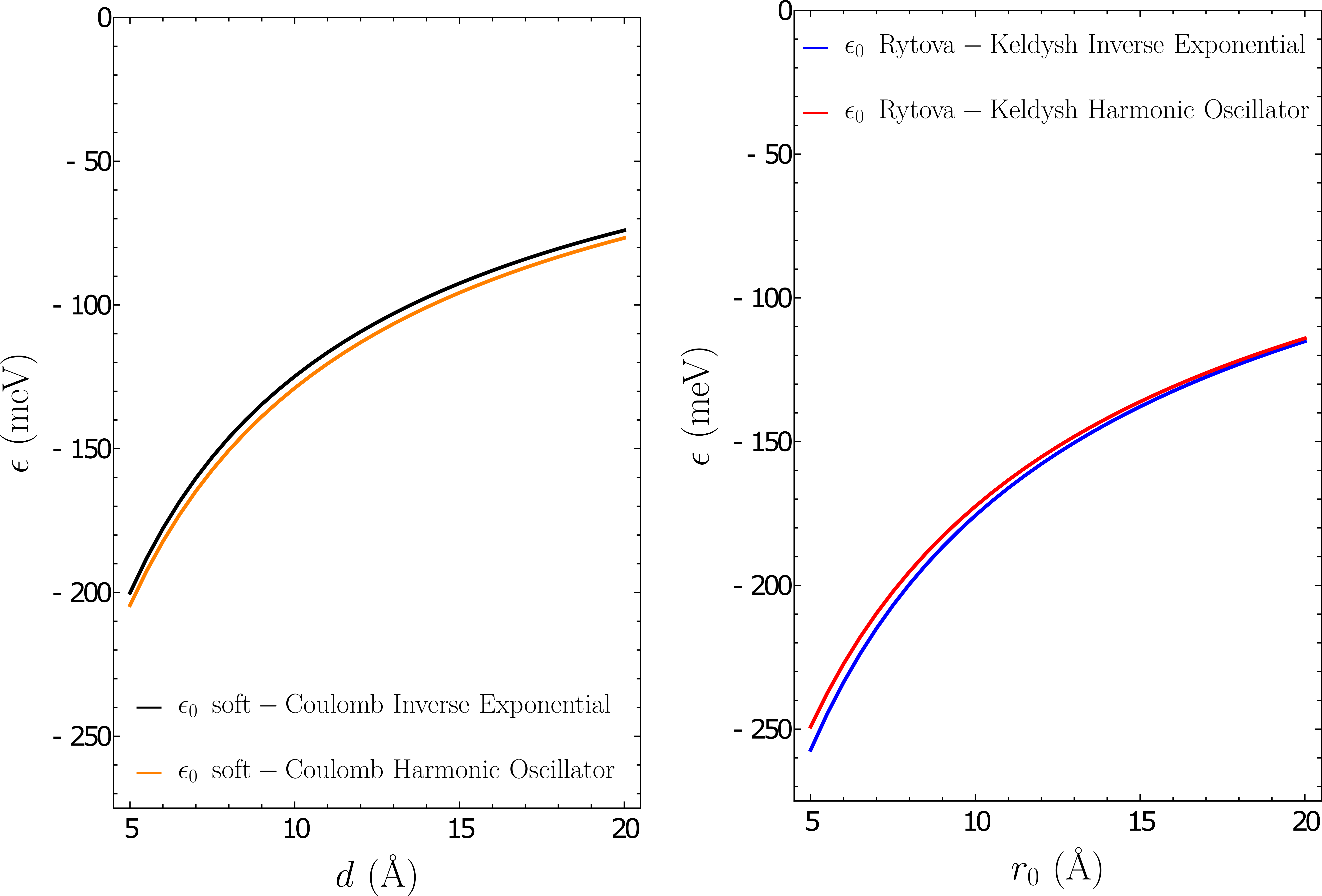
Figure 5: (Left) Comparison of the variational energy calculated for the soft-Coulomb potential with two different ansätze as a function of the separation bias $d\in\left[5,20\right]\,\r{A}$. (Right) Comparison of the variational energy calculated for the Rytova-Keldysh potential with two different ansätze as a function of the screening length $r_{0}\in\left[5,20\right]\,\r{A}$.

Looking at both panels of Fig. 5 we see that both ansätze give very similar ground-state energies. In the case of the soft-Coulomb potential, the harmonic oscillator ansatz gives a slightly smaller energy, whereas the Ritova-Keldysh potential the opposite happens. This inversion is related to the different behavior of the two potentials at the origin: the soft-Coulomb potential does not diverges at the origin whereas the Ritova-Keldysh does. Indeed, the soft-Coulomb potential can be approximated by a parabola at short distances and therefore a harmonic oscillator trial wave function should give a better description to the true wave function of the ground state, as was effectively verified. In the case of a divergent potential at the origin, an inverse exponential ansatz should describe better the ground state wave function.

6 The Wannier–Mott Exciton Model of a TMD Single-Layer

The dielectric constant is generally large in semiconductors, which in turn increases electric screening. This reduces the electron-hole interaction, increasing the radius of the exciton. When this exciton radius is greater than the lattice spacing, the exciton is a Wannier-Mott exciton Wannier_1937 ; mott_basis_1949 . These are typically found in semiconductors with small energy gaps and high dielectric constants, as expected.

Transition-metal dichalcogenides, more specifically their 2D form, have emerged in the fields of electronics and optoelectronics. One of their distinguishing features are the larger-than-usual exciton (and trion) binding energies, almost an order of magnitude larger compared to other bulk semiconductors. These large binding energies imply that many-body interactions are fundamental to determining and understanding the electronic and optoelectronic properties.

Using an equation of motion approach, Have et al.Have_2019 calculated excitonic properties of monolayer TMDs perturbed by an external magnetic field. The obtained results are compared to both the Wannier model for excitons, as well as recent experimental results. A good agreement between the authors’ calculated excitonic transition energies and experimental data is observed, whilst being slightly lower than those calculated via the Wannier exciton model. The authors also show that the effects of the surrounding dielectric environment in the magnetoexciton energy is minimal, as the changes in the exciton energy and the exchange energy correction counteract each other.

To better exemplify this exciton model, as well as compare the results obtained from it against those from first–principles calculations, we will briefly review the work of Zhang et al.zhang_absorption_2014 . In their work, the authors show that the traditional Wannier-Mott exciton model with some modifications is able to appropriately describe the exciton in 2D dichalcogenides. The modifications in question involve taking into account accurate band structures of the conduction and valence bands for large wave-vectors, incorporating phase-space cancellations due to Pauli exclusion in doped materials, as well as taking into account the finite thickness of dichalcogenide monolayers by considering a wave-vector-dependent dielectric constant. With these modifications, the authors study normally incident radiation, discussing the binding energy and the absorption spectrum, both with and without taking into account Pauli blocking.

6.1 Exciton States

Zhang et al.zhang_absorption_2014 consider a system where the initial state $\left|\psi_{i}\right\rangle$ of the semiconductor consists of a completely filled valence band, as well as a conduction band with an electron density $n_{e}$ in accordance with the Fermi-Dirac distribution $f_{c}\left(\mathrm{k}\right)$. This initial state belongs to a thermal ensemble and the average energy of the ground-state ($\left|\psi_{i}\right\rangle$) is $E_{i}$ (i.e., $\left\langle\psi_{i}\right|\hat{H}\left|\psi_{i}\right\rangle=E_{i}$).

Since only excitons with zero in-plane momentum are created by normally incident radiation, an exciton state with zero in-plane momentum can be constructed from the initial state as zhang_absorption_2014

$$\left|\psi_{\mathrm{ex}}\right\rangle=\frac{1}{\sqrt{A}}\sum_{\mathbf{k}}\frac{\phi\left(\mathbf{k}\right)}{N_{\mathrm{ex}}\left(\mathbf{k}\right)}c_{\mathbf{k},\uparrow}^{\dagger}b_{\mathbf{k},\uparrow}\left|\psi_{i}\right\rangle,$$ (18)

where $c_{\mathbf{k},\uparrow},\,b_{\mathbf{k},\uparrow}$ are the destruction operators for the spin-up conduction and valence-band states with momentum $\mathbf{k}$, respectively, and $A$ is the area of the monolayer (normalization factor). The normalization factor $N_{\mathrm{ex}}\left(\mathbf{k}\right)$ equals $\sqrt{1-f_{c}\left(\mathbf{k}\right)}$ and this exciton state is normalized such that $\left\{\left\langle\psi_{\mathrm{ex}}|\psi_{\mathrm{ex}}\right\rangle\right\}_{\mathrm{th}}=1$, where $\left\{\ldots\right\}_{\mathrm{th}}$ represents averaging with respect to the thermal ensemble). The presence of the Fermi-Dirac distribution in Eq. 18 allows the discussion of doped TMDs. In this context, it has been shown that the occuring blueshift of the binding energies depends significantly on the specific doping ($10\,\mathrm{meV}$ in electron-doped samples, while being absent in hole-doped samples) Chang_2019 ; Van_Tuan_2019 . Note that only the $\tau=1$ valley, where the top most valence band is occupied by spin-up $\left(\sigma=1\right)$, has been considered in Eq. (18). Considering spin-down electrons will only multiply the final result by a degeneracy factor $g=2$, due to the contribution from the $\tau=-1$ valley, so no generality is lost when dealing only with spin-up electrons.

The state defined in Eq. 18 is that of a Wannier exciton, as we are assuming that Wannier exciton theory is valid for 2D metal dichalcogenides, and is an eigenstate of the interacting Hamiltonian mahan_many-particle-physics ; Haug_2009

$$\hat{H}= \sum_{\mathbf{k}}E_{c,\mathbf{k}}c_{\mathbf{k}}^{\dagger}c_{\mathbf{k}}+\sum_{\mathbf{k}}E_{v,\mathbf{k}}b_{\mathbf{k}}^{\dagger}b_{\mathbf{k}}+$$

$$+\frac{1}{2}\sum_{\mathbf{k},\mathbf{k}^{\prime},\mathbf{q}\neq 0}V_{\mathbf{q}}\left(c_{\mathbf{k}+\mathbf{q}}^{\dagger}c_{\mathbf{k}^{\prime}-\mathbf{q}}^{\dagger}c_{\mathbf{k}^{\prime}}c_{\mathbf{k}}+\right.$$

$$+\left.b_{\mathbf{k}+\mathbf{q}}^{\dagger}b_{\mathbf{k}^{\prime}-\mathbf{q}}^{\dagger}b_{\mathbf{k}^{\prime}}b_{\mathbf{k}}+2c_{\mathbf{k}+\mathbf{q}}^{\dagger}b_{\mathbf{k}^{\prime}-\mathbf{q}}^{\dagger}b_{\mathbf{k}^{\prime}}c_{\mathbf{k}}\right)$$ (19)

only when $n_{e}=0$. As this is not the case, this state is taken as a variational state, where the function $\phi\left(\mathbf{k}\right)$ can be varied to minimize the expectation value $\left\{\left\langle\psi_{\mathrm{ex}}\right|\hat{H}\left|\psi_{\mathrm{ex}}\right\rangle\right\}_{\mathrm{th}}$. In Eq. 19, $E_{c,\mathbf{k}}$ and $E_{v,\mathbf{k}}$ are the conduction and valence band dispersion relations, respectively, while $V_{\mathbf{q}}$ is the interaction potential.

Manipulating the eigenvalue equation for this Hamiltonian (see Appendix C), the Hermitian eigenvalue equation is

$$\left[E_{\mathrm{ex}}-E_{i}\right]\phi\left(\mathbf{k}\right)=\left[\bar{E}_{c}\left(\mathbf{k}\right)-\bar{E}_{v}\left(\mathbf{k}\right)\right]\phi\left(\mathbf{k}\right)-$$

$$-\frac{\sqrt{1-f_{c}\left(\mathbf{k}\right)}}{A}\sum_{\mathbf{q}}V\left(\mathbf{q}\right)\phi\left(\mathbf{k}-\mathbf{q}\right)\sqrt{1-f_{c}\left(\mathbf{k}-\mathbf{q}\right)}$$ , (20)

where $E_{\mathrm{ex}}$ is the average energy of the state $\left|\psi_{\mathrm{ex}}\right\rangle$ and $E_{\mathrm{ex}}-E_{i}=E_{g}-E_{\mathrm{exb}}$, where $E_{\mathrm{exb}}$ is the exciton binding energy and $E_{\mathrm{g}}$ is the energy gap. The eigenfunctions $\phi_{i}\left(\mathbf{k}\right)$ are defined as orthogonal and $\bar{E}_{c/v}\left(\mathbf{k}\right)$ are the conduction/valence band dispersion relations, including exchange corrections. The dielectric constant $\epsilon\left(q\right)$ is, in general, frequency and wave-vector dependent Ouerdane_2011 and is given by (see the Appendix of Ref. zhang_absorption_2014 )

$$\epsilon\left(q\right)=\epsilon_{2}\frac{1-\frac{\left(1-\epsilon_{2}/\epsilon_{1}\right)\left(1-\epsilon_{2}/\epsilon_{3}\right)}{\left(1+\epsilon_{2}/\epsilon_{1}\right)\left(1+\epsilon_{2}/\epsilon_{3}\right)}e^{-2qd}}{\left[1-\frac{\left(1-\epsilon_{2}/\epsilon_{1}\right)}{\left(1+\epsilon_{2}/\epsilon_{1}\right)}e^{-qd}\right]\left[1-\frac{\left(1-\epsilon_{2}/\epsilon_{3}\right)}{\left(1+\epsilon_{2}/\epsilon_{3}\right)}e^{-qd}\right]}$$ (21)

for a $\mathrm{M}\mathrm{X}_{2}$ monolayer of thickness $d$ and dielectric constant $\epsilon_{2}$ “sandwiched” between materials with dielectric constants $\epsilon_{1},\,\epsilon_{3}$. Asymptotically, this expression can be written as $\epsilon\left(q\right)=\frac{\epsilon_{1}+\epsilon_{3}}{2}$ in the $qd\ll 1$ limit, and $\epsilon\left(q\right)=\epsilon_{2}$ for large wave vectors or very thick monolayers$\left(qd\gg 1\right)$. These limits match those expected considering the varying thickness of the TMD monolayer.

The solutions to Eq. 20 represent bound excitons, as well as electron-hole scattering states. These are, however, excluded since their inclusion leads to modifications in the absorption spectrum near the band edge far from the fundamental exciton line. The authors assume the variational solution

$$\begin{array}[]{ccc}\phi\left(\mathbf{k}\right)=\frac{\sqrt{8\pi}a}{\left[1+\left(ka\right)^{2}\right]^{3/2}}&\implies&\phi\left(\mathbf{r}\right)=\sqrt{\frac{2}{\pi}}\frac{1}{a}e^{-r/a}\end{array},$$ (22)

which is the exact exciton wave function for the Coulomb potential when $n_{e}=0$ and $\epsilon\left(q\right)$ is independent of $q$ Schmitt_Rink_1985 (i.e., local screening). Varying the radius parameter $a$, the eigenvalue $E_{\mathrm{ex}}-E_{i}$ can be estimated.

6.2 Optical Conductivity and Absorption Spectrum

The electronic and optical properties of a TMD are determined by the low energy Hamiltonian of the system. In the case we are considering, this Hamiltonian is valid around the $\mathcal{K}$ and $\mathcal{K}^{\prime}$ points of the hexagonal Brillouin zone, where the band gap is located. Effectively, the low energy Hamiltonian is similar to a Dirac Hamiltonian in 2D, with an additional term due to spin-orbit coupling, induced by the heavy metal atoms. The Hamiltonian near the $\mathcal{K},\,\mathcal{K}^{\prime}$ points is given by

$$H_{0}=\left[\begin{array}[]{cc}\Delta/2&\hbar vk_{-}\\ \hbar vk_{+},&-\Delta/2+\lambda\tau\sigma\end{array}\right],$$ (23)

where $\Delta$ is related to the material band gap, $\sigma=\pm 1$ stands for the electron spin, $\tau=\pm 1$ is the valley index $\left(\mathcal{K},\,\mathcal{K}^{\prime}\right)$, $2\lambda$ is the splitting of the valence band due to spin-orbit coupling, $k_{\pm}=\tau k_{x}\pm ik_{y}$ (the wave vectors are measured from the $\mathcal{K}\,\left(\mathcal{K}^{\prime}\right)$ points), and the velocity parameter $v\approx 5-6\times 10^{5}\,\mathrm{m/s}$ is related to the coupling between the orbitals of neighboring $\mathrm{M}$ atoms.

Zhang et al.zhang_absorption_2014 assume linearly polarized light of frequency $\omega$ and intensity $I_{0}$ incident normally on the $\mathrm{M}\mathrm{X}_{2}$ monolayer. The electric field is obtained directly from Maxwell’s equations and, by definition of the Poynting vector (time averaged for a linearly polarized electromagnetic plane wave), we have

$$I_{0}=\frac{1}{2\eta_{0}}\left|E_{0}\right|^{2}=\frac{A_{0}^{2}\omega^{2}}{2\eta_{0}},$$ (24)

where $\eta_{0}$ is the free-space impedance and $A_{0}$ is the intensity of the vector potential in the monolayer plane.

The interaction between spin-up electrons in the valley $\tau=+1$ and light is given by the Hamiltonian have_excitonic_2019 ; Peres_2010

$$H_{int}\left(t\right) =H_{+}e^{-i\omega t}+\mathrm{h.c.}$$

$$=\frac{eA_{0}}{2m_{0}}\sum_{\mathbf{k}}\vec{P}_{cv}\left(\mathbf{k}\right)\cdot\hat{n}e^{-i\omega t}c_{\mathbf{k},\uparrow}^{\dagger}b_{\mathbf{k},\uparrow}+\mathrm{h.c.},$$ (25)

where $\hat{n}$ is the polarization vector (in the plane of the monolayer), $c_{\mathbf{k},\uparrow},\,b_{\mathbf{k},\uparrow}$ are, respectively, the destruction operators for the spin-up conduction and valence-band states with momentum $\mathbf{k}$, $m_{0}$ is the free-electron mass and $\vec{P}_{cv}\left(\mathbf{k}\right)$ is the momentum matrix element, taken between the conduction and valence bands.

From Fermi’s golden rule, the rate at which excitons are generated by the absorption of light assuming finite broadening $\Gamma_{\mathrm{ex}}$ is given by Glutsch_2004

$$R_{\mathrm{ex}} =\frac{2\pi}{\hbar}\frac{1}{A}\left\{\left|\left\langle\psi_{\mathrm{ex}}\right|\hat{H}_{+}\left|\psi_{\mathrm{i}}\right\rangle\right|^{2}\right\}_{\mathrm{th}}\times$$

$$\quad\times\frac{\hbar\Gamma_{\mathrm{ex}}/\pi}{\left(\hbar\omega_{0}-\hbar\omega\right)^{2}+\left(\hbar\Gamma_{\mathrm{ex}}\right)^{2}},$$ (26)

where $\hbar\omega_{0}=E_{\mathrm{ex}}-E_{\mathrm{i}}$. Directly replacing $H_{+}$ from Eq. 25 and expanding the modulus squared, we obtain

$$\frac{1}{A}\left\{\left|\left\langle\psi_{\mathrm{ex}}\right|\hat{H}_{+}\left|\psi_{\mathrm{i}}\right\rangle\right|^{2}\right\}_{\mathrm{th}} =\left(\frac{eA_{0}}{2m_{0}}\right)^{2}\left|\chi_{\mathrm{ex}}\left(\mathrm{r}=0\right)\right|^{2}$$ (27)

where

$$\chi_{\mathrm{ex}}\left(\mathbf{r}\right)=\int\frac{d^{2}\mathbf{k}}{\left(2\pi\right)^{2}}\phi\left(\mathbf{k}\right)\sqrt{1-f_{c}\left(\mathbf{k}\right)}\left[\vec{P}_{cv}\left(\mathbf{k}\right)\cdot\hat{n}\right]e^{i\mathbf{k}\cdot\mathbf{r}}.$$ (28)

Different processes, such as scattering and inhomogeneous broadening are expected to contribute to the absorption width $\Gamma_{\mathrm{ex}}$. Equation 28 incorporates the effects (reduction in exciton oscillator strength) due to Pauli blocking. The total energy absorption rate from both valleys in the Brillouin zone $\left(\mathcal{K},\,\mathcal{K}^{\prime}\right)$ is given by $2\hbar\omega R_{\mathrm{ex}}$, and can be written in terms of the exciton contribution to the optical conductivity, which is

$$\mathrm{Re}\left\{\sigma_{\mathrm{ex}}\left(\omega\right)\right\} =\frac{2\hbar\omega}{\eta_{0}I_{0}}R_{ex}$$

$$=\frac{e^{2}}{4\hbar}\left\{\frac{8\hbar}{m_{0}^{2}\omega_{0}}\left|\chi_{\mathrm{ex}}\left(\mathbf{r}=0\right)\right|^{2}\times\right.$$

$$\quad\times\left.\frac{\hbar\Gamma_{\mathrm{ex}}}{\left(\hbar\omega_{0}-\hbar\omega\right)^{2}+\left(\hbar\Gamma_{\mathrm{ex}}\right)^{2}}\right\}.$$ (29)

Once the real part of the conductivity has been determined, the imaginary part follows from the Kramers-Kronig relations. The absorption spectrum for normally incident light can be obtained from the optical conductivity Haug_2009 as

$$A\left(\omega\right)\approx\frac{2\mathrm{Re}\left\{\sigma_{\mathrm{ex}}\left(\omega\right)\right\}\eta_{0}}{1+n_{sub}},$$ (30)

where $n_{sub}$ is the refractive index of the substrate (in the case discussed by the authors, quartz).

Ignoring the effects of Pauli blocking and considering the wave-vector-independent expression for the momentum matrix element in Eqs. 26 and 29, the exciton optical conductivity is given by

$$\mathrm{Re}\left\{\sigma_{\mathrm{ex}}\left(\omega\right)\right\} =\frac{2e^{2}v^{2}}{\omega_{0}}\frac{2}{\pi a^{2}}\frac{\hbar\Gamma_{\mathrm{ex}}}{\left(\hbar\omega_{0}-\hbar\omega\right)^{2}+\left(\hbar\Gamma_{\mathrm{ex}}\right)^{2}}$$ (31)

and the product $\left.A\left(\omega\right)\right|_{max}2\hbar\Gamma_{ex}$ by

$$\left.A\left(\omega\right)\right|_{max}2\hbar\Gamma_{ex} =\frac{16\eta_{0}}{1+n_{sub}}\frac{e^{2}v^{2}}{\pi\omega_{0}}\frac{1}{a^{2}}.$$ (32)

By comparison with the extracted peaks, the exciton radius $a$ is found to be around $\sim 16.8\,\text{\AA}$. This radius is much larger than the lattice spacing, thus justifying the validity of the Wannier model. This approach is however too simplistic. A more realistic approach takes trigonal warping into account by adding more terms to $H_{0}$.

Taking into account the wave-vector dependence of the momentum matrix elements (due to trigonal warping), as well as Pauli blocking, the absorption spectrum reads

$$\left.A\left(\omega\right)\right|_{max}2\hbar\Gamma_{ex}=\frac{16\eta_{0}}{1+n_{sub}}\frac{e^{2}}{2m_{0}^{2}\omega_{0}}\left|\chi_{\mathrm{ex}}\left(\mathbf{r}=0\right)\right|^{2},$$ (33)

from which the exciton radius can be extracted given the electron density. For carrier densities around $2-4\times 10^{12}\,\mathrm{cm}^{-2}$, Zhang et al. obtain the exciton radius in the $9.3-8.5\,\text{\AA}$ range, in agreement with first-principles theoretical estimateszhang_absorption_2014 .

In Ref. zhang_absorption_2014 , the absorption spectrum is discussed and compared to the measured spectrum of $\mathrm{Mo}\mathrm{S}_{2}$ at different temperatures. Comparing the calculated spectra against the extracted contributions for the specific materials and excitons in question (at both $T=5\,K$ and $T=90\,K$), Zhang et al. obtain a good fit between the two curves. Furthermore, the individual contributions from both excitons and trions (not discussed in this colloquium) appear to be reliably extractable using this fitting procedure.

6.3 Binding Energy

As the obtained expression for the absorption spectrum has a free parameter, the exciton radius, the resulting curves are superposed against the experimental fits for various temperatures. By matching the peaks, the value for the exciton radius is extracted. The only free parameter in the variational eigenvalue equation becomes the momentum– and frequency–dependent dielectric constant (Eq. 21), which can be obtained by applying the variational principle to Eq.20 using the obtained variational functions in Eq.22, and matching the resulting exciton radii with the values obtained from the absorption peaks. Considering that the top–bottom Sulfur distance in $\mathrm{MoS}_{2}$ is $\sim 3.17\,\text{\AA}$ (the effective monolayer thickness is taken as $d\sim 6\,\text{\AA}$ zhang_absorption_2014 ) and that we have a quartz substrate ($\epsilon_{3}=4$) and $\epsilon_{1}$ as free space ($=1$), the value of $\epsilon_{2}$ for which the exciton radii matches the measured values is $\epsilon_{2}\sim 12$. While rather large, this value matches well with the theoretical estimates for the bulk $\mathrm{MoS}_{2}$ dielectric constant. Furthermore, following Berkelbach et al.Berkelbach_2013 and Cudazzo et al.Cudazzo_2011 , one finds the screening length parameter $r_{0}$. The resulting value, $36\,\text{\AA}$, is in excellent agreement with first-principles calculations by Berkelbach et alBerkelbach_2013 ($30-40\,\text{\AA}$). The variational binding energy for the extracted values is in the $0.28-0.33\,\mathrm{eV}$ range, in good agreement with the first-principles calculations Berkelbach_2013 ; Qiu_2013 .

7 Interlayer Excitons in a TMD: The Harmonic Potential Approximation

Many authors discuss the optical and electronic properties of excitons in TMDs and vdW heterostructures from a numerical point of view, usually by directly integrating the Schrödinger equation with either the Rytova-Keldysh potential (via finite elements, for example). Brunetti et al.brunetti_optical_2018 verify the accuracy of the numerical results for large interlayer separations by approximating the electron-hole interaction as an harmonic potential. As the Schrödinger equation is solvable exactly for this interaction, both the wave function and the energy eigenvalue can be written in close form and used to verify the validity of numerically calculated physical quantities such as the (peak) absorption coefficient and the exciton binding energy.

Among the most recent numerical studies, we mention specifically those by Avalos-Ovando et al.avalos-ovando_lateral_2019 , Scharf et al.Scharf_2019 , Van der Donck et al.van_der_donck_excitons_2017 and Brunetti et al.brunetti_optical_2018 . We will now briefly discuss the results by Brunetti et al..

7.1 The Harmonic Potential Approximation

In the case of interlayer excitons, the modified Rytova-Keldysh potential (defined ahead) shows a minimum at $r=0$ and has a finite value at that point. This happens because interlayer excitons are spatially separated by a distance $d$. Then, we can expand the modified potential around $r=0$ up to second order, leading to the harmonic approximation. In this work brunetti_optical_2018 , the authors discuss the optical absorption of interlayer excitons in a vdW heterostructure. Starting from the oscillator strength for a generic transition

$$f_{i\rightarrow f}=\frac{2\mu\omega_{i\rightarrow f}\left|\left\langle f\right|x\left|i\right\rangle\right|^{2}}{\hbar},$$ (34)

the imaginary part of the electric susceptibility is given by snoke2009solid

$$\mathrm{Im}\left\{\chi\left(\omega\right)\right\}=-\frac{\pi e^{2}}{2\varepsilon_{0}\mu\omega_{0}}\frac{n_{0}}{2h}f_{0}\frac{\Gamma_{\mathrm{ex}}/2}{\left(\omega_{0}^{2}-\omega^{2}\right)^{2}+\left(\Gamma_{\mathrm{ex}}/2\right)^{2}},$$ (35)

where $n_{0}$ is the 2D concentration of excitons in the heterostructure, $h$ is the thickness of one TMD monolayer, $\Gamma_{\mathrm{ex}}$ the homogeneous line-broadening (with physical origin in exciton-phonon interactions), $f_{0}$ represents the oscillator strength for a generic transition, $\omega_{0}$ refers to the respective Bohr angular frequency of the oscillator strength $f_{0}$, and $\mu$ is the exciton reduced mass. Knowing this, the optical absorption coefficient is given by jackson1999classical ; Haug_2009 ($c$ is the speed of light)

$$\alpha\left(\omega\right)=-\frac{\omega}{n\left(\omega\right)c}\mathrm{Im}\left\{\chi\left(\omega\right)\right\},$$ (36)

which can be further simplified assuming the environment interacts weakly with photons in the frequency range of the corresponding optical transition, approximating the refractive index of the environment as $n\left(\omega\right)\approx\sqrt{\varepsilon}$, with $\varepsilon$ being the static dielectric constant of the environment. At the peak, the absorption coefficient is given by

$$\alpha\left(\omega=\omega_{0}\right)=\frac{\pi e^{2}}{2\varepsilon_{0}\mu\sqrt{\varepsilon}c}\frac{n_{0}}{2h}f_{0}\frac{2}{\Gamma_{\mathrm{ex}}},$$ (37)

which is defined by the oscillator strength, and depends on a series of material-specific parameters.

The interlayer modified Rytova-Keldysh potential reads

$$V_{RK}\left(r\right)=-\frac{\pi k}{2r_{0}}\left[H_{0}\left(\frac{\sqrt{r^{2}+d^{2}}}{r_{0}^{2}}\right)-Y_{0}\left(\frac{\sqrt{r^{2}+d^{2}}}{r_{0}^{2}}\right)\right],$$ (38)

with $k=e^{2}/4\pi\epsilon_{0}\kappa$ and $\kappa=\frac{\epsilon_{1}+\epsilon{2}}{2}$ describes the surrounding dielectric medium, is approximated by a harmonic potential by considering the interlayer separation $d$ much larger than the in-plane gyration radius $\left(r_{X}=\sqrt{\left\langle r^{2}\right\rangle}\right.$, that is, the average of $r^{2}$ taken with the exciton wave function). This approximation is given by Berman-2017 ; brunetti_optical_2018

$$V\left(r\right)\approx-V_{0}+\gamma r^{2},$$ (39)

with $r_{0}$ the dielectric screening length and

$$V_{0} =\frac{\pi k}{2r_{0}}\left[H_{0}\left(\frac{d}{r_{0}}\right)-Y_{0}\left(\frac{d}{r_{0}}\right)\right]$$

$$\gamma =-\frac{\pi k}{4r_{0}^{2}d}\left[H_{-1}\left(\frac{d}{r_{0}}\right)-Y_{-1}\left(\frac{d}{r_{0}}\right)\right].$$ (40)

Considering this approximation, the Schrödinger equation can be solved directly in polar coordinates as Edery_2018 ; cohen-tannoudji_quantum_2019

$$\Psi\left(\eta,\varphi\right) =A_{nl}\left(\frac{\hbar}{\mu\omega}\right)^{|l|/2}\eta^{|l|/2}e^{-\eta/2}L_{n}^{|l|}(\eta)\frac{e^{il\varphi}}{\sqrt{2\pi}},$$ (41)

where $\eta=\mu\omega r^{2}/\hbar$, $\omega=\sqrt{2\gamma/\mu}$, $n=0,1,2,\ldots$ and $l=-n,-n+1,\ldots,n-1,n$ are the usual principal and angular momentum quantum numbers, and $L_{b}^{a}\left(x\right)$ is the associate Laguerre polynomial of degree $b$ and order $a$, and

$$A_{nl}=\left(\frac{\mu\omega}{\hbar}\right)^{(|l|+1)/2}\sqrt{\frac{2n!}{\Gamma(n+|l|+1)}},$$ (42)

with $\Gamma(x)$ the gamma-function. The energy eigenvalues present the usual form for the isotropic harmonic oscillator, given by

$$E_{n}=\hbar\left(\frac{2\gamma}{\mu}\right)^{1/2}\left(2n+|l|+1\right)-V_{0}.$$ (43)

This approximation becomes more accurate the more layers are included in the heterostructure (as expected by the assumption of large interlayer separation), and it is verified by comparison with the results from direct numerical integration (through finite elements methods), as well as those obtained experimentally Horng_2018 ; Rahaman2019 or via DFT Kyl_np__2015 .

This approach agrees with the numerical results obtained by Brunetti et al.brunetti_optical_2018 , validating the numerical approach utilized. The eigenenergies and eigenfunctions for interlayer $\left(d\neq 0\right)$ excitons are calculated for a range of material-specific parameters consistent with those from different TMDs. Comparing against existing DFT results Kyl_np__2015 , an agreement to better than $1\%$ is obtained. As such, eigenvalues and optical properties for interlayer excitons can be calculated for different ranges of input parameters consistent with different TMD/h-BN/TMD heterostructures.

In a recent experimental work Horng_2018 , spatially-indirect excitons were observed in a single $\mathrm{Mo}\mathrm{Se}_{2}$ crystal. In bilayer $\mathrm{Mo}\mathrm{Se}_{2}$ encapsulated by h-BN, spatially-indirect excitons are reported to have a binding energy of $153\,\mathrm{meV}$. For the material-dependent parameters provided by Horng_2018 , and using the oscillator strength $f_{0}$ for the transition between the $n=1\rightarrow 2,\,l=0\rightarrow 1$ eigenstates brunetti_optical_2018 , Brunetti’s calculations give a binding energy of $132-140\,\mathrm{meV}$, within $\approx 10\%$ of the reported value.

8 Conclusions and Outlook

The objective of this colloquium was to present an analysis of excitons in 2D materials and vdW heterostructures using the variational method. We have focused our attention in transition metal dichalcogenides that have a direct band gap at the $\cal K$ and $\cal K^{\prime}$ points of the Brillouin zone. In these systems, the electronic and optical properties are described by an effective theory based on the 2D Dirac equation. However, other 2D systems exist presenting indirect band gap between the $\Gamma$ and the M points, such as ZrS₂ and HfS₂ Lau_2019 .

We have first analyzed variational methods for obtaining the binding energy of vdW excitons whose interaction is described by the soft-Coulomb potential. This potential includes a material-dependent parameter which eliminates the divergence of the Coulomb potential at the origin. This material dependent parameter appears in the electrostatic interaction when an electron is in a given layer and the hole is in a different one, a distance $d$ apart from each other. This can happen both in bulk single crystals, due to the layered nature of these materials, or in heterogeneous systems made by staking different 2D materials on top of each other. In simple systems, analytical solutions for soft-Coulomb potential are known, thus allowing for the comparison of the variational approach with exact analytical results.

After presenting the variational method in the context of the soft-Coulomb potential, we considered the Rytova-Keldysh potential. This interaction describes better the scenario of a monolayer transition-metal dichalcogenide both suspended, supported by a substrate, or encapsulated by low-dielectric materials. This potential is mathematically more complex than the soft-Coulomb one. It can, however, be closely approximated by a logarithmic and an inverse-exponential term, which may allow the calculation of the binding energies analytically.

Although we have not considered van der Waals excitons in 2D quantum dots (triangular and hexagonal, as there are no circular TMD systems) the introduced methodology is appropriate to the study of these systems, as wave functions with the correct symmetry can be easily constructed using, for example, group-symmetry arguments.

For connecting with experimental results, both the absorption spectrum and the polarizability of excitons was discussed. These two properties are extremely important in optics since they govern the system’s response to optical impulses. The Stark effect and ionization rate of van der Waals heterostructures have also been considered, as these effects can considerably enhance the photodetection response of photodetectors.

This colloquium does not exhaust all the possibilities of the variational method, with trions and bi-excitons physical properties also being amenable to this type of treatment. Also, the inclusion of a magnetic field causes no difficulties to the method.

Appendix A Exciton dipole matrix element in the Wannier model: two-band system

In this Appendix we show that under specific conditions it is the Fourier transform to real space, at the origin of the relative coordinate, of the exciton wave function in momentum space that determines the dipole matrix element associated with the optical transitions referred in the main text. Furthermore, we will see that this result is indeed an approximation and does not hold in general. This is specially true when the wave function of the electron and the hole are defined by momentum-dependent spinors. Let us consider an exciton with center-of-mass momentum $\mathbf{Q}$. The excitonic wave function reads

$$|\Psi_{X,\mathbf{Q}}\rangle=\frac{1}{\sqrt{A}}\sum_{\mathbf{k}}\phi_{cv}(\mathbf{k})|\psi_{c,\mathbf{k}-\mathbf{Q}/2}^{*},\psi_{v,\mathbf{k}+\mathbf{Q}/2}\rangle,$$ (44)

where $\phi_{cv}(\mathbf{k})$ is the exciton wave function is momentum space and $|\Psi_{X,\mathbf{Q}}\rangle$ represents a sum of Slater determinants with excitons of momentum $\mathbf{k}$. Therefore, we obtain for the dipole matrix element between the ground state, $|0\rangle$ (a Slater determinant), of the TMD and its excited state the result 0080168469

$$\langle 0|\mathbf{\sum_{i}\mathbf{r}_{i}}|\Psi_{X,\mathbf{Q}}\rangle \equiv\mathbf{d}_{0,X}=\frac{1}{\sqrt{A}}\sum_{\mathbf{k}}\phi_{cv}(\mathbf{k})\times$$ (45)

$$\quad\times\int d\mathbf{r}\psi_{c,\mathbf{k}-\mathbf{Q}/2}^{*}(\mathbf{r})\mathbf{r}\psi_{v,\mathbf{k}+\mathbf{Q}/2}(\mathbf{r}),$$

where $\mathbf{r}$ is the relative coordinate and $\sum_{i}\mathbf{r}_{i}$ is a sum over the position of all the electrons in the solid. Defining

$$\mathbf{d}_{c,\mathbf{k}-\mathbf{Q}/2;v,\mathbf{k}+\mathbf{Q}/2}\equiv\int d\mathbf{r}\psi_{c,\mathbf{k}-\mathbf{Q}/2}^{*}(\mathbf{r})\mathbf{r}\psi_{v,\mathbf{k}+\mathbf{Q}/2}(\mathbf{r}),$$ (46)

we obtain

$$\mathbf{d}_{0,X}=\frac{1}{\sqrt{A}}\sum_{\mathbf{k}}\phi_{cv}(\mathbf{k})\mathbf{d}_{c,\mathbf{k}-\mathbf{Q}/2;v,\mathbf{k}+\mathbf{Q}/2}.$$ (47)

Now, consider excitons with zero center of mass momentum, $\mathbf{Q}=0$, described by plane waves. Assuming that the momentum dipole matrix element is weakly dependent on $\mathbf{k}$ in this case, we can approximate

$$\mathbf{d}_{c,\mathbf{k}-\mathbf{Q}/2;v,\mathbf{k}+\mathbf{Q}/2}\simeq\frac{1}{A}\mathbf{d}_{c;v},$$ (48)

such that the exciton dipole moment is given by

$$\mathbf{d}_{0,X} \simeq\frac{1}{\sqrt{A}}\frac{1}{A}\sum_{\mathbf{k}}\phi(\mathbf{k})\mathbf{d}_{c;v}$$

$$=\frac{1}{\sqrt{A}}\chi_{{\rm ex}}(\mathbf{r}=0)\mathbf{d}_{c;v}.$$ (49)

Therefore, we see that it is the Fourier transform to real space (at the origin), $\chi_{{\rm ex}}(\mathbf{r}=0)$, of the exciton wave function in momentum space that determines the optical response of the semiconductor. We note that if the electron and hole wave function cannot be taken as plane waves then extra momentum-dependent factors appear and we cannot obtain the simple result given in Eq. (49). In this case, other states, in addition to the $s-$state (the only one finite at the origin) of the exciton wave function, contribute to the optical response.

Appendix B Derivation of the Rytova-Keldysh potential

In this Appendix, we perform a derivation of a screened potential based on the assumption that the charge fluctuation is proportional to the Laplacian of the potential evaluated in the plane of the 2D material surrounded by vacuum PhysRevB.84.085406 . Such an assumption comes from the following considerations: the induced charge density $\delta n_{2D}\left(\mathbf{r}_{\parallel}\right)$ due to a point charge in the system is given by the 2D polarization in the usual way

$$\delta n_{2D}\left(\mathbf{r}_{\parallel}\right)=-\nabla\cdot\mathbf{P}_{2D},$$ (50)

where the three-dimensional position vector is given by $\mathbf{r}=(\mathbf{r}_{\parallel},z)$, and $\delta n_{2D}$ has units of charge per unit area. The polarization itself is proportional to the total electric field

$$\mathbf{P}_{2D}=-\epsilon_{0}\chi_{2D}\nabla V\left(\mathbf{r}_{\parallel},z=0\right),$$ (51)

with $\chi_{2D}$ having dimensions of length. Therefore,

$$\delta n_{2D}\left(\mathbf{r}_{\parallel}\right)=\epsilon_{0}\chi_{2D}\nabla^{2}V\left(\mathbf{r}_{\parallel},z=0\right).$$ (52)

Let us write Poisson’s equation as:

$$\nabla^{2}V\left(\mathbf{r}\right)=-\frac{e}{\epsilon_{0}}\left[n_{2D,+}+n\left(\mathbf{r}\right)\right],$$ (53)

where $n_{2D,+}$ is the background positive charge density due to the atomic nuclei. We now write the electronic density as $n\left(\mathbf{r}\right)=-n_{2D,-}+\delta\left(\mathbf{r}\right)+\delta\left(z\right)\delta\sigma\left(\mathbf{r}_{\parallel}\right)$, where $n_{2D,-}$ is the neutralizing density of negative charge, $\delta\left(\mathbf{r}\right)$ represents the density of a localized charge and $\delta\left(z\right)\delta\sigma\left(\mathbf{r}_{\parallel}\right)$ is the induced charge density. With these definitions Poisson’s equation reads

$$\nabla^{2}V\left(\mathbf{r}\right) =-\frac{e}{\epsilon_{0}}\left[\delta\left(\mathbf{r}\right)+\delta\left(z\right)\delta\sigma\left(\mathbf{r}_{\parallel}\right)\right]$$

$$=-\frac{e}{\epsilon_{0}}\delta\left(\mathbf{r}\right)-\delta\left(z\right)\chi_{2D}\nabla^{2}V\left(\mathbf{r}_{\parallel},0\right),$$ (54)

where $e\delta\sigma(\mathbf{r}_{\parallel})=\delta n_{2D}(\mathbf{r}_{\parallel})$. Fourier transforming the previous equation we obtain

$$\nabla^{2} \int\frac{d\mathbf{k}}{\left(2\text{$\pi$}\right)^{3}}e^{i\mathbf{k}\cdot\mathbf{r}}V\left(\mathbf{k}\right)=-\frac{e}{\epsilon_{0}}\int\frac{d\mathbf{k}}{\left(2\text{$\pi$}\right)^{3}}e^{i\mathbf{k}\cdot\mathbf{r}}+$$

$$+\chi_{2D}\int\frac{dk_{z}}{2\pi}e^{ik_{z}z}\int\frac{d\mathbf{k}_{\parallel}}{\left(2\text{$\pi$}\right)^{2}}e^{i\mathbf{k_{\parallel}}\cdot\mathbf{r_{\parallel}}}k_{\parallel}^{2}V\left(\mathbf{k_{\parallel}},0\right).$$ (55)

Therefore

$$-\left(k_{\parallel}^{2}+k_{z}^{2}\right)V\left(\mathbf{k}\right)=-\frac{e}{\epsilon_{0}}+k_{\parallel}^{2}\chi_{2D}V\left(\mathbf{k}_{\parallel},z=0\right).$$ (56)

Solving for $V\left(\mathbf{k}\right)$ we obtain

$$V\left(\mathbf{k}\right)=\frac{e}{\epsilon_{0}}\frac{1}{k_{\parallel}^{2}+k_{z}^{2}}-\frac{k_{\parallel}^{2}}{k_{\parallel}^{2}+k_{z}^{2}}\chi_{2D}V\left(\mathbf{k}_{\parallel},z=0\right).$$ (57)

Fourier transforming the previous equation in the $k_{z}$ coordinate (and taking $z=0$) we obtain

$$V\left(\mathbf{k}_{\parallel},z=0\right)=\frac{e}{2\pi\epsilon_{0}}\frac{\pi}{k_{\parallel}}-\frac{\pi}{2\pi}k_{\parallel}\chi_{2D}V\left(\mathbf{k}_{\parallel},z=0\right),$$ (58)

where

$$V\left(\mathbf{k}_{\parallel},z=0\right)=\int_{-\infty}^{\infty}\frac{dk_{z}}{2\pi}V\left(\mathbf{k}_{\parallel},k_{z}\right).$$ (59)

Solving for $V\left(\mathbf{k}_{\parallel},z=0\right)$ we obtain

$$V\left(\mathbf{k}_{\parallel},z=0\right) =\frac{e}{2\epsilon_{0}}\frac{1}{k_{\parallel}}\frac{1}{1+\chi_{2D}k_{\parallel}/2}$$

$$=\frac{e}{2\epsilon_{0}k_{\parallel}}\frac{1}{1+k_{\parallel}/\kappa_{\parallel}},$$ (60)

where $1/\kappa_{\parallel}=\chi_{2D}/2$. The Fourier transform of the potential reads 1979JETPL..29..658K

$$V\left(\mathbf{r}_{\parallel},z=0\right) =\frac{e}{2\epsilon_{0}}\int\frac{d\theta dk_{\parallel}}{(2\pi)^{2}}\frac{e^{i\mathbf{k}_{\parallel}\cdot\mathbf{r}_{\parallel}}\kappa_{\parallel}}{\kappa_{\parallel}+k_{\parallel}}$$

$$=\frac{e\kappa_{\parallel}}{2\epsilon_{0}}\int_{0}^{\infty}\frac{dk_{\parallel}}{2\pi}\frac{J_{0}\left(k_{\parallel}r\right)}{\kappa_{\parallel}+k_{\parallel}}$$

$$=\frac{e\kappa_{\parallel}}{4\pi\epsilon_{0}}\frac{\pi}{2}\left[H_{0}\left(r\kappa_{\parallel}\right)-Y_{0}\left(r\kappa_{\parallel}\right)\right]$$

$$=\frac{e}{4\pi\epsilon_{0}r_{0}}\frac{\pi}{2}\left[H_{0}\left(\frac{r}{r_{0}}\right)-Y_{0}\left(\frac{r}{r_{0}}\right)\right],$$ (61)

where $r_{0}=1/\kappa_{\parallel}$, and $H_{0}\left(x\right)$ and $Y_{0}\left(x\right)$ are the Struve function and the Bessel function of the second kind, respectively.

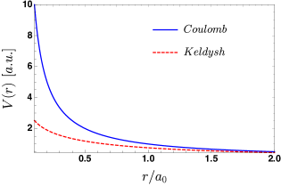
Figure 6: Comparison of the Rytova-Keldysh and Coulomb potentials in arbitrary units.

Appendix C Wannier–Mott variational eigenvalue equation

In this appendix, we will quickly outline the necessary manipulations to obtain Eq. 20 from Eq. 19. Starting with $\left\{\left\langle\psi_{\mathrm{ex}}\right|\hat{H}\left|\psi_{\mathrm{ex}}\right\rangle\right\}_{\mathrm{th}}$, one substitutes in it the definition of Eq. 18. Expanding the resulting equation, one immediately obtains the term proportional to the ground state energy, $E_{i}\sum_{k}\left|\phi\left(k\right)\right|^{2}$ when acting with the Hamiltonian on the ground state. Inspecting the remaining terms individually while utilizing the anti-commutation relations of the creation/destruction operators for each band, the terms proportional to $E_{c,\mathbf{k}}$ and $E_{v,\mathbf{k}}$ simplify almost immediately.

Regarding the interaction terms, we start with

$$V_{\mathbf{q}}c_{\mathbf{k}+\mathbf{q}}^{\dagger}b_{\mathbf{k}^{\prime}-\mathbf{q}}^{\dagger}b_{\mathbf{k}^{\prime}}c_{\mathbf{k}}.$$ (62)

Contracting indices and, again, making use of the anti-commutation relations, this interaction term simplifies to

$$-\sum_{\mathbf{k}^{\prime\prime}}\phi^{*}\left(\mathbf{k}^{\prime\prime}\right)\frac{\sqrt{1-f_{c}\left(\mathbf{k}^{\prime\prime}\right)}}{A}\sum_{\mathbf{q}\neq 0}V_{\mathbf{q}}\phi\left(\mathbf{k}^{\prime\prime}-\mathbf{q}\right)\times$$

$$\times\sqrt{1-f_{c}\left(\mathbf{k}^{\prime\prime}-\mathbf{q}\right)}.$$ (63)

The exchange terms for the conduction band,

$$\frac{1}{2}V_{\mathbf{q}}c_{\mathbf{k}+\mathbf{q}}^{\dagger}c_{\mathbf{k}^{\prime}-\mathbf{q}}^{\dagger}c_{\mathbf{k}^{\prime}}c_{\mathbf{k}},$$ (64)

result in

$$\frac{1}{2}\sum_{\mathbf{k}^{\prime}}\phi^{*}\left(\mathbf{k}^{\prime}\right)\frac{\sqrt{1-f_{c}\left(\mathbf{k}^{\prime}\right)}}{A}\sum_{\mathbf{q}\neq 0}V_{\mathbf{q}}\phi\left(\mathbf{k}^{\prime}-\mathbf{q}\right)\times$$

$$\times\sqrt{1-f_{c}\left(\mathbf{k}^{\prime}-\mathbf{q}\right)},$$ (65)

while those for the valence band,

$$\frac{1}{2}V_{\mathbf{q}}b_{\mathbf{k}+\mathbf{q}}^{\dagger}b_{\mathbf{k}^{\prime}-\mathbf{q}}^{\dagger}b_{\mathbf{k}^{\prime}}b_{\mathbf{k}},$$ (66)

result in

$$-\frac{1}{2}\sum_{\mathbf{k}}\sum_{\mathbf{q}\neq 0}V_{\mathbf{q}}\left|\phi\left(\mathbf{k}\right)\right|^{2}.$$ (67)

Including these exchange terms in the definition of $\bar{E}_{c/v}\left(\mathbf{k}\right)$ (as seen in Eq. 20), the eigenvalue equation becomes

$$\sum_{\mathbf{k}}\phi^{*}\left(\mathbf{k}\right)\left\{\left[\bar{E}_{c,\mathbf{k}}-\bar{E}_{v,\mathbf{k}}\right]\phi\left(\mathbf{k}\right)+E_{i}\phi\left(\mathbf{k}\right)-\right.$$

$$\left.-\frac{\sqrt{1-f_{c}\left(\mathbf{k}\right)}}{A}\sum_{\mathbf{q}}V\left(\mathbf{q}\right)\phi\left(\mathbf{k}-\mathbf{q}\right)\sqrt{1-f_{c}\left(\mathbf{k}-\mathbf{q}\right)}\right\}=$$

$$=\sum_{\mathbf{k}}\phi^{*}\left(\mathbf{k}\right)E_{\mathrm{ex}}\phi\left(\mathbf{k}\right).$$ (68)

Dropping the non-zero common factor $\phi^{*}\left(\mathbf{k}\right)$ while analyzing this sum term-by-term, we obtain the eigenvalue equation of Eq. 20

$$\left[E_{\mathrm{ex}}-E_{i}\right]\phi\left(\mathbf{k}\right)=\left[\bar{E}_{c}\left(\mathbf{k}\right)-\bar{E}_{v}\left(\mathbf{k}\right)\right]\phi\left(\mathbf{k}\right)-$$

$$-\frac{\sqrt{1-f_{c}\left(\mathbf{k}\right)}}{A}\sum_{\mathbf{q}}V\left(\mathbf{q}\right)\phi\left(\mathbf{k}-\mathbf{q}\right)\sqrt{1-f_{c}\left(\mathbf{k}-\mathbf{q}\right)}$$ . (69)

References

- [1] Nicolas Mounet, Marco Gibertini, Philippe Schwaller, Davide Campi, Andrius Merkys, Antimo Marrazzo, Thibault Sohier, Ivano Eligio Castelli, Andrea Cepellotti, Giovanni Pizzi, and Nicola Marzari. Two-dimensional materials from high-throughput computational exfoliation of experimentally known compounds. Nat. Nano., 13(3):246–252, feb 2018.
- [2] R. F. Frindt and A. D. Yoffe. Phys. properties of layer structures : optical properties and photoconductivity of thin crystals of molybdenum disulphide. Proc. R. Soc. Lond. A, 273(1352):69–83, apr 1963.
- [3] E. Fortin and W.M. Sears. Photovoltaic effect and optical absorption in MoS2. J. of Phys. and Chem. of Solids, 43(9):881–884, jan 1982.
- [4] Thomas Mueller and Ermin Malic. Exciton physics and device application of two-dimensional transition metal dichalcogenide semiconductors. npj 2D Mat. and Applications, 2(1):29, December 2018.
- [5] Gang Wang, Alexey Chernikov, Mikhail M. Glazov, Tony F. Heinz, Xavier Marie, Thierry Amand, and Bernhard Urbaszek. Colloquium: Excitons in atomically thin transition metal dichalcogenides. Rev. Mod. Phys., 90:021001, Apr 2018.
- [6] Hongyi Yu, Xiaodong Cui, Xiaodong Xu, and Wang Yao. Valley excitons in two-dimensional semiconductors. National Science Review, 2(1):57–70, 2015.
- [7] R. S. Knox. Introduction to exciton phys. In Collective Excitations in Solids, pages 183–245. Springer US, 1983.
- [8] N.S. Rytova, Alexey Chernikov, and Mikhail Glazov. Screened potential of a point charge in a thin film. Moscow University Phys. Bulletin, 3:30, 01 1967.
- [9] L. V. Keldysh. Coulomb interaction in thin semiconductor and semimetal films. Sov. J. Exp. Theor. Phys. Lett., 29:658, June 1979.
- [10] A. K. Geim and I. V. Grigorieva. Van der Waals heterostructures. Nature, 499(7459):419–425, jul 2013.
- [11] Xi-Ying Dong, Run-Ze Li, Jia-Pei Deng, and Zi-Wu Wang. Interlayer exciton-polaron effect in transition metal dichalcogenides van der Waals heterostructures. J. of Phys. and Chem. of Solids, 134:1–4, nov 2019.
- [12] Kristian Sommer Thygesen. Calculating excitons, plasmons, and quasiparticles in 2D materials and van der Waals heterostructures. 2D Mater., 4(2):022004, jun 2017.
- [13] Matthew N Brunetti, Oleg L Berman, and Roman Ya Kezerashvili. Optical absorption by indirect excitons in a transition metal dichalcogenide/hexagonal boron nitride heterostructure. J. of Phys.: Cond. Matt., 30(22):225001, June 2018.
- [14] Dinh Van Tuan, Min Yang, and Hanan Dery. The Coulomb interaction in monolayer transition-metal dichalcogenides. Phys. Rev. B, 98(12):125308, September 2018. arXiv: 1801.00477.
- [15] J-Z Zhang and J-Z Ma. Two-dimensional excitons in monolayer transition metal dichalcogenides from radial equation and variational calculations. J. of Phys.: Cond. Matt., 31(10):105702, March 2019.
- [16] Benedikt Scharf, Dinh Van Tuan, Igor Žutić, and Hanan Dery. Dynamical screening in monolayer transition-metal dichalcogenides and its manifestations in the exciton spectrum. J. Phys.: Cond. Matt., 31(20):203001, mar 2019.
- [17] Høgni C. Kamban and Thomas G. Pedersen. Interlayer excitons in van der Waals heterostructures: Binding energy, Stark shift, and field-induced dissociation. Scientific Reports, 10(1):5537, December 2020.
- [18] L. S. R. Cavalcante, A. Chaves, B. Van Duppen, F. M. Peeters, and D. R. Reichman. Electrostatics of electron-hole interactions in van der Waals heterostructures. Phys. Rev. B, 97(12), mar 2018.
- [19] K. S. Novoselov, A. K. Geim, S. V. Morozov, D. Jiang, Y. Zhang, S. V. Dubonos, I. V. Grigorieva, and A. A. Firsov. Electric Field Effect in Atomically Thin Carbon Films. Science, 306(5696):666–669, October 2004.
- [20] K. S. Novoselov, A. K. Geim, S. V. Morozov, D. Jiang, M. I. Katsnelson, I. V. Grigorieva, S. V. Dubonos, and A. A. Firsov. Two-dimensional gas of massless Dirac fermions in graphene. Nature, 438(7065):197–200, November 2005.
- [21] Kin Fai Mak, Changgu Lee, James Hone, Jie Shan, and Tony F. Heinz. Atomically thin MoS2: A new direct-gap semiconductor. Phys. Rev. Lett., 105(13):136805, September 2010.
- [22] Andrea Splendiani, Liang Sun, Yuanbo Zhang, Tianshu Li, Jonghwan Kim, Chi-Yung Chim, Giulia Galli, and Feng Wang. Emerging photoluminescence in monolayer MoS2. Nano Lett., 10(4):1271–1275, 2010. PMID: 20229981.
- [23] Ursula Wurstbauer, Bastian Miller, Eric Parzinger, and Alexander W Holleitner. Light–matter interaction in transition metal dichalcogenides and their heterostructures. J. Phys. D: Appl. Phys., 50(17):173001, mar 2017.
- [24] Alexey Chernikov, Timothy C. Berkelbach, Heather M. Hill, Albert Rigosi, Yilei Li, Ozgur Burak Aslan, David R. Reichman, Mark S. Hybertsen, and Tony F. Heinz. Exciton binding energy and nonhydrogenic rydberg series in monolayer WS2. Phys. Rev. Lett., 113:076802, Aug 2014.
- [25] Kin Fai Mak, Keliang He, Changgu Lee, Gwan Hyoung Lee, James Hone, Tony F. Heinz, and Jie Shan. Tightly bound trions in monolayer MoS2. Nat. Mat., 12(3):207–211, dec 2012.
- [26] Keliang He, Nardeep Kumar, Liang Zhao, Zefang Wang, Kin Fai Mak, Hui Zhao, and Jie Shan. Tightly bound excitons in monolayer WSe2. Phys. Rev. Lett., 113(2), jul 2014.
- [27] Di Xiao, Gui-Bin Liu, Wanxiang Feng, Xiaodong Xu, and Wang Yao. Coupled spin and valley phys. in monolayers of MoS2 and other group-VI dichalcogenides. Phys. Rev. Lett., 108(19), may 2012.
- [28] A. K. Geim and I. V. Grigorieva. Van der Waals heterostructures. Nature, 499(7459):419–425, jul 2013.
- [29] Zongyou Yin, Hai Li, Hong Li, Lin Jiang, Yumeng Shi, Yinghui Sun, Gang Lu, Qing Zhang, Xiaodong Chen, and Hua Zhang. Single-layer MoS2 phototransistors. ACS Nano, 6(1):74–80, 2012. PMID: 22165908.
- [30] Zongyou Yin, Hai Li, Hong Li, Lin Jiang, Yumeng Shi, Yinghui Sun, Gang Lu, Qing Zhang, Xiaodong Chen, and Hua Zhang. Single-layer MoS2 phototransistors. ACS Nano, 6(1):74–80, dec 2011.
- [31] Andreas Pospischil, Marco M. Furchi, and Thomas Mueller. Solar-energy conversion and light emission in an atomic monolayer p–n diode. Nat. Nano., 9(4):257–261, mar 2014.
- [32] Marco M. Furchi, Andreas Pospischil, Florian Libisch, Joachim Burgdörfer, and Thomas Mueller. Photovoltaic effect in an electrically tunable van der Waals heterojunction. Nano Lett., 14(8):4785–4791, July 2014.
- [33] M. Amani, D.-H. Lien, D. Kiriya, J. Xiao, A. Azcatl, J. Noh, S. R. Madhvapathy, R. Addou, S. KC, M. Dubey, K. Cho, R. M. Wallace, S.-C. Lee, J.-H. He, J. W. Ager, X. Zhang, E. Yablonovitch, and A. Javey. Near-unity photoluminescence quantum yield in MoS2. Science, 350(6264):1065–1068, nov 2015.
- [34] Xiao-Xiao Zhang, Ting Cao, Zhengguang Lu, Yu-Chuan Lin, Fan Zhang, Ying Wang, Zhiqiang Li, James C. Hone, Joshua A. Robinson, Dmitry Smirnov, Steven G. Louie, and Tony F. Heinz. Magnetic brightening and control of dark excitons in monolayer WSe2. Nat. Nano., 12(9):883–888, jun 2017.
- [35] M R Molas, C Faugeras, A O Slobodeniuk, K Nogajewski, M Bartos, D M Basko, and M Potemski. Brightening of dark excitons in monolayers of semiconducting transition metal dichalcogenides. 2D Mat., 4(2):021003, jan 2017.
- [36] Benedikt Scharf, Tobias Frank, Martin Gmitra, Jaroslav Fabian, Igor Žutić, and Vasili Perebeinos. Excitonic Stark effect in MoS2 monolayers. Phys. Rev. B, 94(24):245434, December 2016.
- [37] Sten Haastrup, Simone Latini, Kirill Bolotin, and Kristian S. Thygesen. Stark shift and electric-field-induced dissociation of excitons in monolayer MoS2 and hBN/MoS2 heterostructures. Phys. Rev. B, 94(4):041401, July 2016.
- [38] Mathieu Massicotte, Fabien Vialla, Peter Schmidt, Mark B. Lundeberg, Simone Latini, Sten Haastrup, Mark Danovich, Diana Davydovskaya, Kenji Watanabe, Takashi Taniguchi, Vladimir I. Fal’ko, Kristian S. Thygesen, Thomas G. Pedersen, and Frank H. L. Koppens. Dissociation of two-dimensional excitons in monolayer WSe2. Nat. Comm., 9(1):1633, December 2018.
- [39] Albert F. Rigosi, Heather M. Hill, Yilei Li, Alexey Chernikov, and Tony F. Heinz. Probing interlayer interactions in transition metal dichalcogenide heterostructures by optical spectroscopy: MoS2/WS2 and MoSe2/WSe2. Nano Lett., 15(8):5033–5038, jul 2015.
- [40] Timothy C. Berkelbach and David R. Reichman. Optical and excitonic properties of atomically thin transition-metal dichalcogenides. Annu. Rev. Cond. Matt. Phys., 9(1):379–396, mar 2018.
- [41] N. Aquino, G. Campoy, and A. Flores-Riveros. Accurate energy eigenvalues and eigenfunctions for the two-dimensional confined hydrogen atom. Int. J. Quant. Chem., 103(3):267–277, 2005.
- [42] Federico Grasselli. Variational approach to the soft-Coulomb potential in low-dimensional quantum systems. Am. J. Phys., 85(11):834–839, November 2017.
- [43] Manuel Iñarrea, Víctor Lanchares, Jesús F. Palacián, Ana I. Pascual, J. Pablo Salas, and Patricia Yanguas. Effects of a soft-core coulomb potential on the dynamics of a hydrogen atom near a metal surface. Comm. in Nonlinear Science and Numerical Simulation, 68:94–105, March 2019.
- [44] V. Shahnazaryan, I. Iorsh, I. A. Shelykh, and O. Kyriienko. Exciton-exciton interaction in transition-metal dichalcogenide monolayers. Phys. Rev. B, 96(11), sep 2017.
- [45] Shahnaz Aas and Ceyhun Bulutay. Strain dependence of photoluminescence and circular dichroism in transition metal dichalcogenides: a kp analysis. Opt. Express, 26(22):28672, oct 2018.
- [46] Chenhao Jin, Emma C. Regan, Aiming Yan, M. Iqbal Bakti Utama, Danqing Wang, Sihan Zhao, Ying Qin, Sijie Yang, Zhiren Zheng, Shenyang Shi, Kenji Watanabe, Takashi Taniguchi, Sefaattin Tongay, Alex Zettl, and Feng Wang. Observation of moiré excitons in WSe2/WS2 heterostructure superlattices. Nature, 567(7746):76–80, feb 2019.
- [47] Andres Castellanos-Gomez. Black phosphorus: Narrow gap, wide applications. J. Phys. Chem. Lett., 6(21):4280–4291, oct 2015.
- [48] M.-Y. Li, Y. Shi, C.-C. Cheng, L.-S. Lu, Y.-C. Lin, H.-L. Tang, M.-L. Tsai, C.-W. Chu, K.-H. Wei, J.-H. He, W.-H. Chang, K. Suenaga, and L.-J. Li. Epitaxial growth of a monolayer WSe2-MoS2 lateral p-n junction with an atomically sharp interface. Science, 349(6247):524–528, jul 2015.
- [49] Amit S. Pawbake, Mahendra S. Pawar, Sandesh R. Jadkar, and Dattatray J. Late. Large area chemical vapor deposition of monolayer transition metal dichalcogenides and their temperature dependent raman spectroscopy studies. Nanoscale, 8(5):3008–3018, 2016.
- [50] Wonbong Choi, Nitin Choudhary, Gang Hee Han, Juhong Park, Deji Akinwande, and Young Hee Lee. Recent development of two-dimensional transition metal dichalcogenides and their applications. Materials Today, 20(3):116–130, apr 2017.
- [51] Pavel V. Ratnikov. Excitons in planar quantum wells based on transition metal dichalcogenides. Phys. Rev. B, 102(8), aug 2020.
- [52] A J Chaves, R M Ribeiro, T Frederico, and N M R Peres. Excitonic effects in the optical properties of 2D materials: an equation of motion approach. 2D Mat., 4(2):025086, April 2017.
- [53] J. Have, N. M. R. Peres, and T. G. Pedersen. Excitonic magneto-optics in monolayer transition metal dichalcogenides: From nanoribbons to two-dimensional response. Phys. Rev. B, 100(4):045411, July 2019.
- [54] J. C. G. Henriques, G. Catarina, A. T. Costa, J. Fernández-Rossier, and N. M. R. Peres. Excitonic magneto-optical Kerr effect in two-dimensional transition metal dichalcogenides induced by spin proximity. Phys. Rev. B, 101(4):045408, January 2020.
- [55] J C G Henriques, G B Ventura, C D M Fernandes, and N M R Peres. Optical absorption of single-layer hexagonal boron nitride in the ultraviolet. J. of Phys.: Cond. Matt., 32(2):025304, January 2020.
- [56] M V Durnev and M M Glazov. Excitons and trions in two-dimensional semiconductors based on transition metal dichalcogenides. Physics-Uspekhi, 61(9):825–845, sep 2018.
- [57] M. Van der Donck, M. Zarenia, and F. M. Peeters. Excitons, trions, and biexcitons in transition-metal dichalcogenides: Magnetic-field dependence. Phys. Rev. B, 97(19):195408, May 2018.
- [58] Andres Castellanos-Gomez, Leonardo Vicarelli, Elsa Prada, Joshua O Island, K L Narasimha-Acharya, Sofya I Blanter, Dirk J Groenendijk, Michele Buscema, Gary A Steele, J V Alvarez, Henny W Zandbergen, J J Palacios, and Herre S J van der Zant. Isolation and characterization of few-layer black phosphorus. 2D Mater., 1(2):025001, jun 2014.
- [59] J-Z Zhang and J-Z Ma. Two-dimensional excitons in monolayer transition metal dichalcogenides from radial equation and variational calculations. J. Phys.: Cond. Matt., 31(10):105702, jan 2019.
- [60] J. Stark. Beobachtungen über den effekt des elektrischen feldes auf spektrallinien. i. quereffekt. Ann. Phys., 348(7):965–982, 1914.
- [61] Barry Simon. The definition of molecular resonance curves by the method of exterior complex scaling. Phys. Lett. A, 71(2-3):211–214, apr 1979.
- [62] C. William McCurdy, Carrie K. Stroud, and Matthew K. Wisinski. Solving the time-dependent schrödinger equation using complex-coordinate contours. Phys. Rev. A, 43(11):5980–5990, jun 1991.
- [63] Xiaoping Hong, Jonghwan Kim, Su-Fei Shi, Yu Zhang, Chenhao Jin, Yinghui Sun, Sefaattin Tongay, Junqiao Wu, Yanfeng Zhang, and Feng Wang. Ultrafast charge transfer in atomically thin MoS2/WS2 heterostructures. Nat. Nano., 9(9):682–686, aug 2014.
- [64] L. Meckbach, T. Stroucken, and S. W. Koch. Influence of the effective layer thickness on the ground-state and excitonic properties of transition-metal dichalcogenide systems. Phys. Rev. B, 97(3), jan 2018.
- [65] Rajeev Kumar, Ivan Verzhbitskiy, Francesco Giustiniano, Themistoklis P H Sidiropoulos, Rupert F Oulton, and Goki Eda. Interlayer screening effects in a van der Waals heterobilayer. 2D Mater., 5(4):041003, aug 2018.
- [66] Fabien Vialla, Mark Danovich, David A Ruiz-Tijerina, Mathieu Massicotte, Peter Schmidt, Takashi Taniguchi, Kenji Watanabe, Ryan J Hunt, Marcin Szyniszewski, Neil D Drummond, Thomas G Pedersen, Vladimir I Fal’ko, and Frank H L Koppens. Tuning of impurity-bound interlayer complexes in a van der Waals heterobilayer. 2D Mater., 6(3):035032, may 2019.
- [67] Simon Ovesen, Samuel Brem, Christopher Linderälv, Mikael Kuisma, Tobias Korn, Paul Erhart, Malte Selig, and Ermin Malic. Interlayer exciton dynamics in van der Waals heterostructures. Communications Physics, 2(1), February 2019.
- [68] Bastian Miller, Alexander Steinhoff, Borja Pano, Julian Klein, Frank Jahnke, Alexander Holleitner, and Ursula Wurstbauer. Long-lived direct and indirect interlayer excitons in van der Waals heterostructures. Nano Lett., 17(9):5229–5237, aug 2017.
- [69] Høgni C. Kamban and Thomas G. Pedersen. Field-induced dissociation of two-dimensional excitons in transition metal dichalcogenides. Phys. Rev. B, 100(4), jul 2019.
- [70] Haining Wang, Changjian Zhang, Weimin Chan, Christina Manolatou, Sandip Tiwari, and Farhan Rana. Radiative lifetimes of excitons and trions in monolayers of the metal dichalcogenide MoS2. Phys. Rev. B, 93(4), jan 2016.
- [71] Galan Moody, Chandriker Kavir Dass, Kai Hao, Chang-Hsiao Chen, Lain-Jong Li, Akshay Singh, Kha Tran, Genevieve Clark, Xiaodong Xu, Gunnar Berghäuser, Ermin Malic, Andreas Knorr, and Xiaoqin Li. Intrinsic homogeneous linewidth and broadening mechanisms of excitons in monolayer transition metal dichalcogenides. Nat. Comm., 6(1), sep 2015.
- [72] B. Han, C. Robert, E. Courtade, M. Manca, S. Shree, T. Amand, P. Renucci, T. Taniguchi, K. Watanabe, X. Marie, L. E. Golub, M. M. Glazov, and B. Urbaszek. Exciton states in monolayer MoSe2 and MoTe2 probed by upconversion spectroscopy. Phys. Rev. X, 8(3), sep 2018.
- [73] E. Courtade, M. Semina, M. Manca, M. M. Glazov, C. Robert, F. Cadiz, G. Wang, T. Taniguchi, K. Watanabe, M. Pierre, W. Escoffier, E. L. Ivchenko, P. Renucci, X. Marie, T. Amand, and B. Urbaszek. Charged excitons in monolayer WSe2: Experiment and theory. Phys. Rev. B, 96(8), aug 2017.
- [74] Changjian Zhang, Haining Wang, Weimin Chan, Christina Manolatou, and Farhan Rana. Absorption of light by excitons and trions in monolayers of metal dichalcogenide MoS2: Experiments and theory. Phys. Rev. B, 89(20):205436, May 2014.
- [75] M. Van der Donck, M. Zarenia, and F. M. Peeters. Excitons and trions in monolayer transition metal dichalcogenides: A comparative study between the multiband model and the quadratic single-band model. Phys. Rev. B, 96(3):035131, July 2017.
- [76] M. Van der Donck and F. M. Peeters. Interlayer excitons in transition metal dichalcogenide heterostructures. Phys. Rev. B, 98(11):115104, September 2018.
- [77] Claudia Ruppert, Ozgur Burak Aslan, and Tony F. Heinz. Optical properties and band gap of single- and few-layer MoTe2 crystals. 14(11):6231, 2014.
- [78] M. A. Semina. Excitons and trions in bilayer van der Waals heterostructures. Phys. Sol. Stat., 61(11):2218–2223, nov 2019.
- [79] Josep Planelles. Simple correlated wave-function for excitons in 0D, quasi-1D and quasi-2D quantum dots. Theor. Chem. Accounts, 136(7):81, July 2017.
- [80] N. Lundt, E. Cherotchenko, O. Iff, X. Fan, Y. Shen, P. Bigenwald, A. V. Kavokin, S. Höfling, and C. Schneider. The interplay between excitons and trions in a monolayer of MoSe2. Appl. Phys. Lett., 112(3):031107, jan 2018.
- [81] R.B. Bhat. Flexural vibration of polygonal plates using characteristic orthogonal polynomials in two variables. J. of Sound and Vibration, 114(1):65–71, January 1987.
- [82] K. M. Liew and K. Y. Lam. A Set of Orthogonal Plate Functions for Flexural Vibration of Regular Polygonal Plates. J. of Vibration and Acoustics, 113(2):182–186, April 1991.
- [83] M F C Martins Quintela and J M B Lopes dos Santos. A polynomial approach to the spectrum of dirac–weyl polygonal billiards. Journal of Physics: Condensed Matter, 33(3):035901, oct 2020.
- [84] Jerry W. Brown and Harold N. Spector. Exciton binding energy in a quantum-well wire. Phys. Rev. B, 35(6):3009–3012, feb 1987.
- [85] Yuan ping Feng and Harold N. Spector. Exciton energies as a function of electric field: Confined quantum stark effect. Phys. Rev. B, 48(3):1963–1966, jul 1993.
- [86] Okikazu Akimoto and Eiichi Hanamura. Excitonic molecule. I. Calculation of the binding energy. J. Phys. Soc. Jpn., 33(6):1537–1544, dec 1972.
- [87] Rodney Loudon. One-dimensional hydrogen atom. Am. J. Phys., 27(9):649–655, dec 1959.
- [88] J C G Henriques, G B Ventura, C D M Fernandes, and N M R Peres. Optical absorption of single-layer hexagonal boron nitride in the ultraviolet. J. Phys.: Cond. Matt., 32(2):025304, oct 2019.
- [89] Pierluigi Cudazzo, Ilya V. Tokatly, and Angel Rubio. Dielectric screening in two-dimensional insulators: Implications for excitonic and impurity states in graphane. Phys. Rev. B, 84:085406, Aug 2011.
- [90] S. Schmitt-Rink and C. Ell. Excitons and electron-hole plasma in quasi-two-dimensional systems. J. of Luminescence, 30(1-4):585–596, feb 1985.
- [91] Høgni C. Kamban, Thomas G. Pedersen, and Nuno M. R. Peres. Anisotropic stark shift, field-induced dissociation, and electroabsorption of excitons in phosphorene. Phys. Rev. B, 102:115305, September 2020.
- [92] Gregory H. Wannier. The structure of electronic excitation levels in insulating crystals. Phys. Rev., 52(3):191–197, aug 1937.
- [93] N. F. Mott. The Basis of the Electron Theory of Metals, with Special Reference to the Transition Metals. Proc. Phys. Soc.. Sec. A, 62(7):416–422, July 1949.
- [94] J. Have, G. Catarina, T. G. Pedersen, and N. M. R. Peres. Monolayer transition metal dichalcogenides in strong magnetic fields: Validating the wannier model using a microscopic calculation. Phys. Rev. B, 99(3), jan 2019.
- [95] Yao-Wen Chang and David R. Reichman. Many-body theory of optical absorption in doped two-dimensional semiconductors. Phys. Rev. B, 99(12), mar 2019.
- [96] Dinh Van Tuan, Benedikt Scharf, Zefang Wang, Jie Shan, Kin Fai Mak, Igor Žutić, and Hanan Dery. Probing many-body interactions in monolayer transition-metal dichalcogenides. Phys. Rev. B, 99(8), feb 2019.
- [97] Gerald D. Mahan. Many-particle physics. Physics of solids and liquids. Plenum Press, 2nd ed edition, 1990.
- [98] Stephan W. Koch Hartmut Haug. Quantum Theory of Optical and Electronic Properties of Semiconductors. World Scientific Publishing Company, 4 edition, 2004.
- [99] H. Ouerdane. Analytic model of effective screened coulomb interactions in a multilayer system. J. Appl. Phys., 110(7):074905, oct 2011.
- [100] N. M. R. Peres, R. M. Ribeiro, and A. H. Castro Neto. Excitonic effects in the optical conductivity of gated graphene. Phys. Rev. Lett., 105(5), jul 2010.
- [101] Stephan Glutsch. Excitons in Low-Dimensional Semiconductors. Springer Berlin Heidelberg, 2004.
- [102] Timothy C. Berkelbach, Mark S. Hybertsen, and David R. Reichman. Theory of neutral and charged excitons in monolayer transition metal dichalcogenides. Phys. Rev. B, 88(4), jul 2013.
- [103] Pierluigi Cudazzo, Ilya V. Tokatly, and Angel Rubio. Dielectric screening in two-dimensional insulators: Implications for excitonic and impurity states in graphane. Phys. Rev. B, 84(8), aug 2011.
- [104] Diana Y. Qiu, Felipe H. da Jornada, and Steven G. Louie. Optical spectrum of MoS2: Many-body effects and diversity of exciton states. Phys. Rev. Lett., 111(21), nov 2013.
- [105] O Ávalos Ovando, D Mastrogiuseppe, and S E Ulloa. Lateral heterostructures and one-dimensional interfaces in 2D transition metal dichalcogenides. J. of Phys.: Cond. Matt., 31(21):213001, May 2019.
- [106] D. W. Snoke. Solid state physics : essential concepts. Addison-Wesley, San Francisco, 2009.
- [107] John Jackson. Classical electrodynamics. Wiley, New York, 1999.
- [108] Oleg L. Berman, Godfrey Gumbs, and Roman Ya. Kezerashvili. Bose-Einstein condensation and superfluidity of dipolar excitons in a phosphorene double layer. Phys. Rev. B, 96:014505, Jul 2017.
- [109] Ariel Edery and Philippe Laporte. First and second-order relativistic corrections to the two and higher-dimensional isotropic harmonic oscillator obeying the spinless salpeter equation. J. Phys. Comm., 2(2):025024, feb 2018.
- [110] Bernard Cohen-Tannoudji, Frank Laloe, and Diu Claude. Quantum Mechanics: volume 3. Wiley, 12 2019.
- [111] Jason Horng, Tineke Stroucken, Long Zhang, Eunice Y. Paik, Hui Deng, and Stephan W. Koch. Observation of interlayer excitons in MoSe2 single crystals. Phys. Rev. B, 97(24), jun 2018.
- [112] Mahfujur Rahaman, Christian Wagner, Ashutosh Mukherjee, Adan Lopez-Rivera, Sibylle Gemming, and Dietrich R T Zahn. Probing interlayer excitons in a vertical van der waals p-n junction using a scanning probe microscopy technique. Journal of Physics: Condensed Matter, 31(11):114001, January 2019.
- [113] Ilkka Kylänpää and Hannu-Pekka Komsa. Binding energies of exciton complexes in transition metal dichalcogenide monolayers and effect of dielectric environment. Phys. Rev. B, 92(20), nov 2015.
- [114] Ka Wai Lau, Caterina Cocchi, and Claudia Draxl. Electronic and optical excitations of two-dimensional ZrS2 and HfS2 and their heterostructure. Phys. Rev. Mat., 3(7), jul 2019.
- [115] G.F. Bassani, G.P. Parravicini, and R.A. Ballinger. Electronic States and Optical Transitions in Solids. International Series of Monographs on solid state physics. Pergamon Press, New York, 1975.