Reinforcement Learning of Causal Variables Using Mediation Analysis

Abstract

We consider the problem of acquiring causal representations and concepts in a reinforcement learning setting. Our approach defines a causal variable as being both manipulable by a policy, and able to predict the outcome. We thereby obtain a parsimonious causal graph in which interventions occur at the level of policies. The approach avoids defining a generative model of the data, prior pre-processing, or learning the transition kernel of the Markov decision process. Instead, causal variables and policies are determined by maximizing a new optimization target inspired by mediation analysis, which differs from the expected return. The maximization is accomplished using a generalization of Bellman’s equation which is shown to converge, and the method finds meaningful causal representations in a simulated environment.

Introduction

Hard open problems in reinforcement learning, such as distributional shift, generalization from small samples, disentangled representations and counter-factual reasoning, are intrinsically related to causality (Schölkopf 2019). Furthermore, causal representations have been emphasized as central to concept acquisition and knowledge representation (Tenenbaum et al. 2011).

Statistical causal analysis, as developed and popularized by Judea Pearl, assumes that data arises as transformations of noise sources according to a causal graph (Pearl 2009). From a practical perspective, describing data generatively as arising from non-linear transformations of i.i.d. noise is an approach that underlies the most successful machine learning models today (Shrestha and Mahmood 2019). Such an approach has been successfully applied for example in fast concept acquisition (Tenenbaum et al. 2011; Lake, Salakhutdinov, and Tenenbaum 2015), as well as in control (Deisenroth and Rasmussen 2011; Levine et al. 2016).

Our approach differs from these in terms of the scale of modeling, a term coined by Peters, Janzing, and Schölkopf (2017):

Although traditional examples of causal modeling, such as the $\textsc{smoking}\rightarrow\textsc{tar deposits}\rightarrow\textsc{cancer}$ example (Pearl and Mackenzie 2018), do offer a generative process of the few variables included in the analysis, they do not offer a generative process of the underlying temporal phenomena (i.e. patient history). The variables are said to be in a descriptive relationship to the underlying phenomena, to emphasize that they are not identified as high-level variables in a generative process, but rather features computed from a more complicated underlying phenomena.

The reduction of the data-generating process to a few abstract primitives in a causal relationship is central to concept acquisition (Tenenbaum et al. 2011), and more broadly to knowledge representation (Davis, Shrobe, and Szolovits 1993).

We aim to answer the following question: Can we automatically learn a parsimonious causal model which is descriptive, rather than generative, of the underlying problem, while still capturing relevant causal knowledge?

To illustrate, consider the Doorkey environment, fig. 1. The agent must pick up the key, open the door and go to the goal state in order to receive the reward. Instead of identifying a generative process of the agent moving around the maze, our approach identifies a binary causal variable (for instance, whether the door is opened or not) and builds a small causal graph representing the causal relationship between the identified variable, policy choice and return. The agent is thereby imbued with the causal knowledge that the identified variable is in a causal relationship with the return.

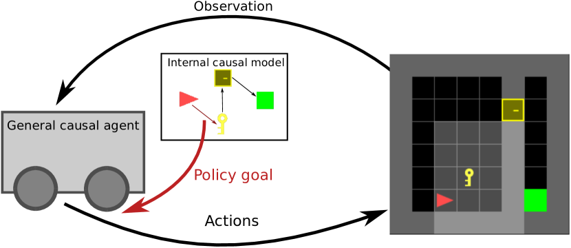
Figure 1: In the Doorkey environment, the agent (red) must learn to pick up a key to open the door and get to the goal. Our causal agent learns a small, coarse-grained causal network, and uses it when training its policy.

Our approach has two central features: First, that we do not identify a causal variable as a latent variable in a generative model of the data, or as a latent factor which arises from maximizing the expected return with respect to the policy. Instead, we replace the expected return with an alternative maximization target, the natural indirect effect (NIE), which is maximized to identify a causal variable. Second, the approach naturally ensures a candidate causal variable represents a feature of the environment the agent can manipulate, thereby ensuring the information is relevant for the agent. This distinguishes between relevant causal concepts and irrelevant ones. In the Doorkey example (fig. 1), a variable corresponding to being one step away from the goal would be a necessary cause for completing the environment. However, it would be no easier to manipulate such a variable than simply reaching the goal state.

To optimize the NIE in a reinforcement learning setting, we apply suitable generalizations of Bellman’s equation. This allows us to apply most actor-critic methods, and specifically, to use an off-policy method based on the $V$-trace estimator (Espeholt et al. 2018).

Related Work:

Determining causal variables has previously been examined in image data from a latent-variable perspective  (Besserve et al. 2020; Lopez-Paz et al. 2017) and time-series signals, using (temporal) state aggregation (Zhang, Gong, and Schölkopf 2015). However, these approaches apply a latent-variable criteria which is distinct from ours. The problem of determining causal variables has also been investigated from a fairness-perspective, see Zhang and Bareinboim (2018).

In a reinforcement-learning setting, the option-critic architecture considers state-dependent policies similar to ours, but from a non-causal perspective Bacon, Harb, and Precup (2017), and Zhang et al. (2019) learn a state representation using sufficient statistics criteria. Determining latent states to best explain the observations is closely related to the reward machine architecture (Camacho et al. 2019; Icarte et al. 2018), which learns binary feature-vector representations in logical, rather than causal, relationships. Nabi, Kanki, and Shpitser (2018) learn policies that optimize a path-specific effect, which is a generalization of the indirect effect. Our approach is different, since we learn both a causal variable and the manipulation policies jointly using a causal criteria.

In recent work, reinforcement learning has been applied for causal discovery in graphs with pre-defined variables, using meta-learning (Dasgupta et al. 2019) and active learning (Amirinezhad, Salehkaleybar, and Hashemi 2020), for example. Wang, Yang, and Wang (2020) consider confounded observational data in a reinforcement learning setting, and their approach is noteworthy as they suggest a modified $Q$-learning update. These approaches, however, consider just a handful of variables that can be observed (and manipulated), which is a different setup than the one considered herein.

Methods

Consider a general $\gamma$-discounted episodic Markov decision problem in which states, actions and rewards at time steps $t=0,1,\dots,T$ are denoted $S_{t}$, $A_{t}$ and $R_{t+1}$ respectively, and the goal is to maximize the expectation of the return $v_{\pi}(s)=\mathbb{E}_{\pi}\left[G_{t}\mid S_{t}=s\right]$ where $G_{t}=\sum_{k=9}^{\infty}\gamma^{k}R_{t+k+1}$. The expectation is with respect to the behavior policy $\pi(a|s)=\textrm{Pr}(A_{t}=a|S_{t}=s)$. For easier interpretation, the examples involve sparse reward $+1$, given at the end of the episode in case of successful termination.

Mediation Analysis

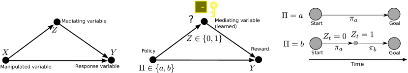
Figure 2: Left: A mediation analysis diagram in which a cause/effect $X\rightarrow Y$ is mediated by a variable $Z$. Center: Application to reinforcement learning: The variable $X$ corresponds to a choice between two policies, the effect $Y$ is the return, and $Z$ is a (learned) variable which influences $Y$. We wish to quantify how the policy choice influences $Y$ through the variable $Z$. Right: $\Pi=a$ indicates that we follow a baseline policy $\pi_{a}$. This is compared to a policy $\Pi=b$ obtained by following the policy $\pi_{b}$ until the first time $t$ where $Z_{t}=1$ occurs, after which we follow $\pi_{a}$. Both $\pi_{a},\pi_{b}$, and the distribution of $Z_{t}$, needs to be learned.

Mediation analysis (Alwin and Hauser 1975; Pearl 2012) deals with decomposing the total causal effect, $p(Y=y|\mathrm{do}(X=x))$, a treatment variable $X$ exerts an outcome variable $Y$ into different causal pathways, which may pass through intermediate mediating variables.

In the simplest setting (see fig. 2, left), $X$ could be whether a school pupil received extracurricular studies, while $Y$ is their academic performance at the end of the year, and the mediating variable $Z$ could correspond to extra study time.

Mediation analysis allows us to quantify the extent to which a third variable, such as $Z$, mediates the effect of $X$ on $Y$. The most important measure is the natural indirect effect (Pearl 2012, 2001), which measures the extent to which $X$ influences $Y$, solely through $Z$. For a transition of $X=x$ (starting value) to $X=x^{\prime}$ (manipulated value), it is defined as expected change in $Y$, affected by holding $X$ constant at its natural value $X=x$, and changing $Z$ to the value it would have attained had $X$ been set to $X=x^{\prime}$. This quantity involves a nested counter-factual, and cannot be estimated in general; however, for specific causal diagrams, it has a closed-form expression. For instance, in the simple case given in fig. 2 (left), it is defined as (Pearl 2001):

$$\textrm{NIE}_{x\rightarrow x^{\prime}}(Y)=\sum_{z}\mathbb{E}\left[Y|x,z\right][P(z|x^{\prime})-P(z|x)].$$ (1)

The NIE has intuitively appealing properties: It is large when $Z$ is highly influenced by our choice of manipulation $X=x,x^{\prime}$, meaning that $Z$ is easy to manipulate, and the first term reflects that $Z$ should influence the outcome $Y$. The product implies a trade-off between these two effects. In our application, we let $X=\Pi$ denote our choice of policy, and then use the NIE to index good (versus bad) choices of the observable variable $Z$ and policies $\Pi$. Hence, we hypothesize that by maximizing the NIE, rather than the expected return, we can determine relevant causal variables, which correspond to useful concepts for the agent.

Causes and Effects in Reinforcement Learning

The most natural causal variable to include in a causal diagram is the expected return $Y=G_{0}$, since manipulating $Y$, and therefore learning which variables are relevant for manipulating $Y$, should remain the eventual goal of the agent.

Since we consider causal variables as aggregates of many individual states, no single action can reasonably be considered a treatment variable. Rather, we consider a treatment equivalent to the choice to follow policy $\Pi=a$ rather than $\Pi=b$.

In the following, we focus on the simplest possible case, in which the mediating variable $Z$ is binary, with the meaning that $Z=1$, if the event which $Z$ corresponds to took place during an episode (and otherwise $Z=0$). This is analogous to how smoking is true if the person was smoking at some point in the period covered by a study. We therefore define $Z$ as a stopped process

$$Z=\max\{Z_{0},Z_{1},\dots Z_{T}\dots\}.$$ (2)

where $Z_{t}\in\{0,1\}$ for $n=0,1,\dots,T$ denotes whether $Z$ became true at time $t$. $Z_{t}$ is assumed to only depend on the state, and have distribution $\textrm{Bern}\left(\Phi(s_{t})\right)$. With these definitions, the causal pathway $\Pi\rightarrow Z\rightarrow Y$ denotes that the choice of policy $\Pi$ influences $Y$ by obtaining or making true $Z$, whereas $\Pi\rightarrow Y$ means the choice of policy alone influences $Y$, regardless of $Z$.

Example:

Consider the Doorkey environment from fig. 1. The graphs $\Pi\rightarrow Z\rightarrow Y$ or $\Pi\rightarrow Y$ would reflect either that our choice of $\Pi$ affects the reward $Y$ through $Z$, or that the variable $Z$ is irrelevant, and only the choice of policy matters. The outcome depends on the choice of policy and definition of $Z$.

The combined policy:

Inspired by the traditional relationship between $X$ and $Z$ in mediation analysis, we assume that if $\Pi=a$ then the agent follows a policy $\pi_{a}$ which is trained to simply maximize $Y$, and that otherwise, if $\Pi=b$, the agent follows a policy $\pi_{b}$ which attempts to make $Z$ true (i.e. it is trained with $Z$ as the reward signal). To obtain a well-defined policy for all states, the $\Pi=b$ policy switches back to $\pi_{a}$ once $Z=1$, see fig. 2 (right). In other words, we assume that the agent at time step $t$ follows the policy:

$$\pi=\begin{cases}\pi_{a}&\mbox{if $\Pi=a$ }\\ \left(1-Z_{0:t}\right)\pi_{b}+Z_{0:t}\pi_{a}&\mbox{if $\Pi=b$. }\end{cases}$$ (3)

where $Z_{0:t}=\max\{Z_{0},\dots,Z_{t}\}$. Since $Z$ and $\Pi$ are binary, the NIE from eq. 1 simplifies to (Pearl 2001):

NIE $$=\left(\mathbb{E}\left[Y|Z=1,\pi_{a}\right]-\mathbb{E}\left[Y|Z=0,\pi_{a}\right]\right)$$

$$\quad\times\left(P(Z=1|\pi_{b})-P(Z=1|\pi_{a})\right).$$ (4)

Conditioning on $\pi_{a}$ or $\pi_{b}$ means that the actions are generated from the given policy.

The NIE has the intuitively appealing property of being separated into a product of two simpler terms, which must both be large for the NIE to be large. The first involves the return, but only conditional on policy $\pi_{a}$. A high value of the NIE implies an increased chance of successful completion of the environment, when $Z=1$ relative to $Z=0$.

The second term involves both policies, but uses $Z$ as a reward signal, which is computed during the episode, and will therefore often be known before the episode is completed. Since this is the only term which involves $\pi_{b}$, it induces a modular policy, in which $\pi_{b}$ is trained on a simpler problem.

The NIE excludes certain trivial definitions of $Z$. For instance, if $Z=Y$ in the Doorkey example, the first term would be maximal. However, in this case, $\pi_{a}$ and $\pi_{b}$ would be trained on the same target, and so the second term should be zero. On the other hand, if $Z$ is trained to match states visited by $\pi_{b}$, which are incidental to the reward, it will not result in a high NIE, due to the first term.

Optimizing the NIE involves two challenges unfamiliar from traditional reinforcement learning: (i) The first term involves expectations conditional on $Z$. (ii) The NIE is optimized both with respect to $Z$ and to $\pi_{b}$.

We overcome these by combining two ideas. First, we express the conditional terms using suitable generalizations of Bellman’s equation. Secondly, since we optimize policies based on data collected from other policies, we use $V$-trace estimates of the relevant quantities (Espeholt et al. 2018).

Bellman Updates

The value function satisfies the Bellman equation $v_{\pi}(s)=\mathbb{E}\left[R_{t+1}+\gamma v_{\pi}(S_{t+1})\mid S_{t}=s\right]$. On comparison with the terms in eq. 4, we see that the NIE involves conditional expectations. While we could attempt to simply divide the observations according to $Z$ and train two value functions, this method would not provide a way to learn $Z$ itself. To do so, we consider an alternative recursive relationship between the conditional expressions.

For times $t\notin\{0,\dots,T\}$ we define $Z_{t}=0$. This allows us to introduce the variables

$$Z_{t}^{\infty}=\max\{Z_{t},Z_{t+1},\dots,\}$$ (5)

which are true, provided $Z_{t^{\prime}}=1$ occurs at a time step following $t$. Note that $Z=Z_{0}^{\infty}$.

Analogous to $v_{t}$, we define the value functions:

$$v^{\infty}_{t}(s_{t}) =P(Z^{\infty}_{t}=1|S_{t}=s_{t},Z_{t-1}=0),$$ (6)

$$v^{z}_{t}(s_{t}) =\mathbb{E}[G_{t}|S_{t}=s_{t},Z_{t}^{\infty}=z,Z_{t-1}=0].$$ (7)

Note that the expressions are conditional on $Z_{t-1}=0$. The first denotes that the event $Z=1$ will happen in the future given it has not occurred yet, and the second the expected return, given that $Z$ has not happened yet, and either will not $z=0$, or will $z=1$ occur in the future. Note that $v^{z}_{0}(s_{0})=\mathbb{E}\left[G_{0}|Z=z,s_{0}\right]$ and $v^{\infty}_{0}(s_{0})=P(Z=1|s_{0})$ corresponds to the terms in eq. 4. The value functions satisfy the recursions (see appendix):

$$v^{\infty}_{t}(s_{t}) =\Phi(s_{t})+\bar{\Phi}(s_{t})\mathbb{E}\left[v^{\infty}_{t+1}(S_{t+1})|s_{t}\right],$$ (8a)

$$v^{1}_{t}(s_{t}) =\frac{V(s_{t})\Phi(s_{t})}{V_{t}^{\infty}(s_{t})}$$ (8b)

$$+\frac{1\!-\!\Phi(s_{t})}{V_{t}^{\infty}(s_{t})} \mathbb{E}\left[v^{\infty}_{t+1}(S_{t+1})\left(R_{t+1}+\gamma v^{1}_{t+1}(S_{t+1})\right)\mid s_{t}\right],$$

$$v^{0}_{t}(s_{t}) =\frac{1-\Phi(s_{t})}{1\!-\!v_{t}^{\infty}(s_{t})}$$ (8c)

$$\times\mathbb{E}[\ (1- v_{t+1}^{\infty}(S_{t+1}))(R_{t+1}+\gamma v^{0}_{t+1}(S_{t+1}))\mid s_{t}].$$

The new recursions have the same structure as Bellman’s equation, but contain mutually dependent terms. If $v_{t}^{\infty}$ and $v_{t}$ were exactly estimated, the iterative policy evaluation methods corresponding to eqs. 8b and 8c would easily be found to be contractions with constant $\gamma$, but the updates also converge when $v^{z}$, $v^{\infty}$ and $v$ are all bootstrapped. A proof can be found in the appendix.

Theorem 1 (Convergence, informal)

Assuming $\gamma<1$ and $0<\Phi<1$, all states/actions are visited infinitely often, and $v_{\pi},v^{\infty}_{\pi},v^{z}_{\pi}$ in eq. 8 are all replaced by randomly initialized bootstrap estimates. Then, (i) the operators eqs. 8b and 8c converge at a geometric rate to the true values $v^{z}_{\pi}$, and (ii) the corresponding online method obtained by replacing the expectations with sample estimates, converges to the true values, provided the learning rates satisfy Robbins-Monro conditions.

Off-Policy Learning Using $V$-Trace Estimators

The overall approach is to learn neural approximations of $v^{\infty}$, $v$ and $v^{z}$, as defined in eq. 8. This is most easily done by observing that the Bellman-like recursions in eq. 8 all have the form:

$$v_{t}(s_{t}) =\mathbb{E}_{\mu}\left[H_{t}(s_{t},S_{n+1})+G_{t}(s_{t},S_{t+1})v_{t+1}(S_{t+1}))\middle|s_{t}\right]$$ (9)

where actions are generated using a behavioral policy $\mu$. Expanding the right-hand side $n$ times, allows us to define the $n$-step return (Espeholt et al. 2018):

$$v_{t}(s_{t}) =\mathbb{E}\left[\sum_{i=t}^{t+n-1}H_{i}\prod_{\ell=t}^{i-1}G_{\ell}+v_{t+n}(S_{t+n})\prod_{\ell=t}^{t+n-1}G_{\ell}\middle|s_{k}\right],$$ (10)

which reduces to eq. 9 if $n=1$. Supposing the current target policy is $\pi$, experience is collected from the behavior policy $\mu$, and then eq. 10 can be used as an estimate of the return, corresponding to $\pi$, by using importance sampling. To reduce variance, we use a $V$-trace type estimator, inspired by Espeholt et al. (2018):

$$V_{t}(s_{t}) =v(s_{t})+\sum_{i=t}^{t+n-1}\left(\prod_{\ell=t}^{i-1}c_{\ell}G_{\ell}\right)\delta_{i}$$ (11a)

$$\delta_{i} =\rho_{i}\left[H_{i}(s_{i},s_{i+1})+G_{i}v(S_{i+1})-v(S_{i})\right]$$ (11b)

where $c_{\ell}$ and $\rho_{k}$ are truncated importance sampling weights:

$$\rho_{t}=\min\left\{\bar{\rho},\frac{\pi(a_{t}|s_{t})}{\mu(a_{t}|s_{t})}\right\},\ c_{t}=\min\left\{\bar{c},\frac{\pi(a_{t}|s_{t})}{\mu(a_{t}|s_{t})}\right\},$$

and $\bar{\rho}\geq\bar{c}$ are parameters of the method. In the on-policy case, where $\mu=\pi$, the $V$-trace estimate eq. 11a reduces to $\sum_{i=t}^{t+n-1}H_{i}\prod_{\ell=t}^{i-1}G_{\ell}+v_{t+n}\prod_{\ell=t}^{t+n-1}G_{\ell}$, and is therefore a direct estimate of eq. 9. In the general case, the method provides a biased estimate, when $\bar{\rho},\bar{c}<\infty$, but analogous to Espeholt et al. (2018), the stationary value function can be analytically related to the true value function. The result is summarized as: (see the appendix for further details)

Algorithm 1 Causal learner

1:  Initialize policy networks $\pi_{a}$ and $\pi_{b}$ (and corresponding critic networks)

2:  Initialize networks $v$, $v^{0}$, $v^{1}$, $v^{\infty}$ to estimate $v_{\pi}$, $v^{z}_{\pi}$, and $V^{\infty}_{\pi}$

3:  Initialize causal variable network $\Phi$

4:  repeat

5:     Collect experience from $\pi_{a}$ and add to replay buffer

6:     Sample experience from replay buffer $\tau$

7:     Train $\pi_{a}$ (and critic) using AC2

8:     Calculate reward signal for $\pi_{b}$ from $\tau$ using eq. 14 and train $\pi_{b}$ (and critic)

9:     Train $v$, $v^{z}$, $v^{\infty}$ using $n$-step $V$-trace estimates eq. 11a, computed using eq. 13, using definitions of $H_{t}$ and $G_{t}$ implied by eq. 8 and experience $\tau$

10:     Train parameters in causal variable network $\Phi$ by maximizing eq. 4, where each term has been replaced by the respective $V$-trace estimate computed using eqs. 8 and 11a

11:  until forever

Theorem 2 ($V$-trace convergence, informal)

Assume that experience is generated by a behavior policy $\mu$, that $\gamma<1$, $0<\Phi<1$, all states/actions are visited infinitely often, and that $v_{\pi},v^{\infty}_{\pi},v^{z}_{\pi}$ in eq. 8 are all replaced by randomly initialized bootstrap estimates. Then, if we apply eq. 11a iteratively  on the bootstrap estimate of $V^{z}$

$$V^{z}(s)\leftarrow_{\alpha}V^{z}(s)+\sum_{t=0}^{\infty}\prod_{\ell=0}^{t-1}c_{\ell}G_{\ell}^{z}\delta_{\ell},$$ (12)

where $H_{\ell}^{z}$ and $G^{z}_{\ell}$ are computed using $V$-trace estimates of $v_{\pi}$ and $v^{\infty}_{\pi}$, it implies that $V^{z}$ converges to a biased estimate of $v^{z}_{\pi}$, and if $\bar{\rho},\bar{c}\rightarrow\infty$, then $V^{z}\rightarrow v_{\pi}^{z}$.

To practically compute the $V$-trace estimates, we start from $T$ and proceed to $t$:

$$V_{t}=v_{t}+\delta_{t}+G_{t}c_{t}(V_{t+1}-v_{t+1}).$$ (13)

Combined Method

The policy $\pi_{b}$ in eq. 3 is trained in an episodic environment to maximize $Z$. Since the variable $Z$ is multiplicative over individual time steps, we train $\pi_{b}$ by decomposing the multiplicative cost using a stick-breaking construction:

$$r_{t+1}^{b}=\Phi(s_{t})\prod_{k=0}^{t-1}(1-\Phi(s_{k})),$$ (14)

which satisfies $\sum_{t=0}^{\infty}r_{t+1}=P(Z=1|\tau)$. Training on this reward signal means that the policy $\pi_{b}$ will attempt to maximize the term $P(Z=1|\pi_{b})-P(Z=1|\pi_{a})$ in eq. 4. We can therefore train both $\pi_{a}$ and $\pi_{b}$ with an actor-critic method, using their respective reward signals, whereby the critics estimate of the return are trained against the $V$-trace estimate, as computed using eq. 13.

To maximize the NIE with respect to $\Phi$, we introduce networks $v$, $v^{z}$ and $v^{\infty}$, to approximate $v_{\pi}$, $v^{\infty}_{\pi}$ and $v^{z}_{\pi}$. These are trained using ordinary gradient descent against their $V$-trace targets, computed by eq. 13. The same $V$-trace estimates can be used to re-write the NIE in eq. 4, to an expression which directly depends on $\Phi$, and can therefore be trained using stochastic gradient descent. For instance, $\mathbb{E}[Y|Z=1,\Pi=a,s_{0}]=v_{\pi_{a}}^{1}(s_{0})$ is equivalent to $V^{z=1}_{t}(s_{0})$, computed using eq. 13, and the definitions of $H_{t}$ and $G_{t}$ implied by eq. 8b, and $\mathbb{E}\left[Z=1|\Pi=a\right]$ can be replaced by $V_{0}^{\infty}$, computed using eq. 8a. The pseudo-code of the method can be found in algorithm 1. Note that to prevent premature convergence, and speed up convergence when both factors in the NIE are small, we train on a surrogate cost function which includes entropy terms for $\Phi$, $\pi_{a}$ and $\pi_{b}$. Full details can be found in the appendix.

Experiments

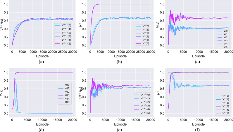
Figure 3: (a-b) Trace plots of $v^{1}$ and $v^{\infty}$ for the tabular Twostage environment obtained using eq. 10, with a given $\Phi$. (c-f) Estimates with neural function approximators for the value functions in the Twostage environment, while $\Phi$ is being learned.

We test the value function recursions in eq. 8 on a simple Markov reward process dubbed Twostage corresponding to an idealized version of the Doorkey environment. In Twostage, the states are divided into two sets $S_{A}$ and $S_{B}$. The initial state is always in $S_{A}$, and the environment can either transition within sets ($S_{A}\rightarrow S_{A}$, $S_{B}\rightarrow S_{B}$) with a fixed probability, or from set $S_{A}$ to $S_{B}$, with a fixed probability. From $S_{B}$, there is a chance to terminate successfully with a reward of $+1$, and from all states there is a chance to terminate unsuccessfully with a reward of $0$.

The transition from states in $S_{A}$ to $S_{B}$, creates a bottleneck distinguishing successful and unsuccessful episodes, much like unlocking the door in the Doorkey environment. The transition probabilities are chosen such that $p(R=1|s\in S_{B})=p(s\in S_{B}|s\in S_{A})=\frac{2}{3}$ and $p(R=1|s\in S_{A})=\frac{4}{9}$, see the appendix for further details.

Tabular Learning

As a first example, we will consider simple estimation of the conditional expectations, using the Bellman recursions. We condition on whether the state enters $S_{B}$ at a later time, i.e. $\mathbb{E}[Y|\mbox{$s_{t}\in S_{B}$ for some $t>0$},S_{0}=s_{0}]$, which is equivalent to $v^{1}(s_{0})$, since we define $\Phi(s)=1_{S_{B}}(s)$. In this case, the Bellman updates from eq. 8) for a transition $S_{t}=s$ to $S_{t+1}=s^{\prime}$, $R_{t+1}=r$ are

$$V(s) \underset{\alpha}{\leftarrow}r+\gamma V(s^{\prime})$$

$$V^{\infty}(s) \underset{\alpha}{\leftarrow}\Phi(s)+(1-\Phi(s))V^{\infty}(s^{\prime})$$ (15)

$$\!\!V^{1}(s) \underset{\alpha}{\leftarrow}\frac{V(s)\Phi(s)\!+\!(1\!-\!\Phi(s))V^{\infty}(s_{t})\left(r\!+\!\gamma V^{1}(s^{\prime})\right)}{V^{\infty}(s)}$$

As anticipated by theorem 1, iterating these updates, the value functions converge to their analytically expected values, as can be seen in figs. 3 and 3, in which we plot $v^{1}$ and $v^{\infty}$. The dashed lines represent the true (analytical) values, and the different colored lines represent the different states. In the case of $v^{1}$, the expectation estimated is the probability of successful completion, given that we begin in any state and at some point enter $S_{B}$; in other words, the information we condition on is something which only occurs at a later point in the episode, from the perspective of an observation $s\in S_{A}$, and therefore the correct estimation of this probability is not simply a matter of computing the return for a state starting in $S_{B}$.

Learning $\Phi$ Using $V$-Trace Estimation

The second example extends the Twostage example to also learn the causal variable $\Phi$ using algorithm 1. Since the environment is a MRP, we discard terms involving $\pi_{b}$, and the objective $\Delta_{Y}$ therefore becomes:

$$\mathbb{E}\left[Y|Z\!=\!1\right]\!-\!\mathbb{E}\left[Y|Z\!=\!0\right]\!=\!\mathbb{E}_{s_{0}}\left[V^{1}(s_{0})\!-\!V^{0}(s_{0})\right].$$ (16)

The expectation is unrolled, using the $V$-trace approximation, and directly optimized with respect to the parameters $(w_{s})_{s}$ of $\Phi$, using the parameterization $\Phi(s)=\frac{1}{1+\exp(-w_{s})}$.

The value function approximation is quickly learned (see fig. 3), showing convergence to the analytical values. The quantities $V^{\infty}$ and $V^{z}$ both depend on $\Phi$, and will therefore only begin to converge after $\Phi$ begins to converge (see fig. 3). Since the conditional expectations $V^{z}$ depend on $V^{\infty}$, they will converge relatively slower, but both will eventually converge to their expected value when the learning rate is annealed, see fig. 3.

Causal Learning and the Doorkey Environment

To apply algorithm 1 to the Doorkey environment, we first have to parameterize the states. The environment has $|\mathcal{A}|=5$ actions, and we consider a fully-observed variant of the environment. We choose the simplest possible encoding, in which each tile, depending on its state, is one-hot encoded as an 11-dimensional vector. This means that an $n\times n$ environment is encoded as an $n\times n\times 11$-dimensional sparse tensor, and we include a single one-hot encoded feature to account for the player orientation. Further details can be found in the appendix. Episode length is 60 steps.

Since the environment encodes orientation, player position and goal position separately, and since specific actions must be used when picking up the key and opening the door, the environment is surprisingly difficult to explore and generalize in. We train an agent using A2C (Mnih et al. 2016) with 1-hidden-layer fully connected neural networks, which results in a completion rate of about $0.25$ within the episode limit. We also attempted to train an agent using the Option-Critic framework (Bacon, Harb, and Precup 2017), a relevant comparison to our method, but failed to learn options which solved the environment better than chance.

After an initial training of $\pi_{a}$, we train $\Phi$ and $\pi_{b}$ by maximizing the NIE, using algorithm 1. Training parameters can be found in the supplementary material. To obtain a fair evaluation on separate test data, we simulate the method on $200$ random instances of the Doorkey environment, and use Monte-Carlo roll-outs of the policies $\pi_{a}$ and $\pi_{b}$ to estimate the quantities $\mathbb{E}\left[Z=1\mid\Pi=a\right]$, $\mathbb{E}\left[Z=1\mid\Pi=b\right]$. This allows us to estimate the NIE on a separate test set.

To examine whether the obtained definition of $Z$ is non-trivial, we compare it against a natural alternative that learns $Z$ by maximizing the cross-entropy of $Z$ and $Y$,

$$-\mathbb{E}_{\tau}\left[Y(\tau)\log P(Z=z|\tau)\right].$$ (17)

Since $Y$ is binary, this corresponds to determining $\Phi$ as the binary classifier which separates successful ($Y=1$) episodes from unsuccessful episodes ($Y=0$), i.e. ensures that the first factor of the NIE eq. 16 is large.

Method	$\mathbb{E}[Y\mid Z=1]$	$\mathbb{E}[Y\mid Z=0]$	$\Delta_{Y}$	$\mathbb{E}_{\pi_{a}}[Z]$	$\mathbb{E}_{\pi_{b}}[Z]$	NIE
Causal Learner	$0.410(30)\text{\,}$	$0.000()\text{\,}$	$0.410(30)\text{\,}$	$0.550(20)\text{\,}$	$0.790(20)\text{\,}$	$0.098(10)\text{\,}$
Cross-entropy	$0.560(80)\text{\,}$	$0.130(30)\text{\,}$	$0.430(100)\text{\,}$	$0.270(40)\text{\,}$	$0.270(30)\text{\,}$	$0.011(8)\text{\,}$

Table 1: Performance of causal agent on the Doorkey environment and standard deviation of the mean.

The results of both methods can be found in table 1 (results averaged over 10 restarts with different seeds). The causal learner obtains a value of the NIE that is significantly different from zero in all runs. While the absolute value is small, this can be attributed to the NIE being a product of two factors which are both small. Considering the first two terms, we observe that the causal variable $Z=1$ is a necessary condition for completing the environment, while the corresponding variable for the cross-entropy target can be false, yet the agent is still able to successfully complete the environment.

We also notice that the cross-entropy based learner outperforms the causal target, in terms of obtaining a proper separation between good versus bad trajectories, i.e. a higher value of $\Delta_{Y}$. This is expected, since cross-entropy is an efficient cost-function for a binary classification problem.

However, the causal variable $Z$, which is learned by the cross-entropy learner, does not present a suitable target for the policy $\pi_{b}$. Indeed, the variable $Z$ becomes true at the same rate under $\pi_{a}$ and $\pi_{b}$ (all policies are trained using the same settings). This can be accounted for by recalling that the environment is random, and that the variable $Z$ learned by the causal learner represents a relatively stable feature of the environment (such as picking up the key, opening the door, etc.), whereas the cross-entropy trained variable $Z$ corresponds to a combination of features in the environment which presents a less suitable optimization target.

To obtain insight in the causal variable we learn, we plot $P(Z=1)$ both against the reward, and whether the door was opened in this particular run (jitter added for easier visualization). The results can be found in fig. 4. As indicated, the learned causal variable correlates well with whether the door is opened or not, and not as well with the total reward. In other words, the method is able to learn that the feature of whether the agent has opened the door acts as a mediating cause in terms of completing the environment. This is a natural result, considering this task is necessary in order for the agent to complete the environment.

The fact that the causal variable corresponds to a meaningful objective, is reinforced by examining the total reward obtained from either following policy $\Pi=a$, or the joint policy $\Pi=b$ (see table 2). Although the difference is slight, we observe a small increase in accumulated reward for the joint policy.

Method	$\mathbb{E}[Y|\Pi=a]$	$\mathbb{E}[Y|\Pi=b]$
Causal Learner	$0.240(20)\text{\,}$	$0.300(30)\text{\,}$
Cross-entropy	$0.230(20)\text{\,}$	$0.240(10)\text{\,}$

Table 2: Reward obtained in the Doorkey environment.

Conclusion

Since all causal conclusion depends on assumptions that are not testable in observational studies (Pearl et al. 2009), it is natural to ask why we are justified in believing that a particular method finds a causal representation of the environment.

In work involving pre-defined variables, such justification can be found either through external distributional assumptions about the relationship between the structure of the model and the data it generates (Spirtes et al. 2000), or because the model belongs to a class of models of which so many examples have been observed, that meta-learning allows the structure to be identified (Dasgupta et al. 2019).

In contrast, our work assumes a specific causal diagram which, along with the definition of $Z$ and $Y$, ensures that $Z$ is imbued with a natural interpretation as the mediating causal factor of the causal pathway from $X$ to $Y$.

A more fundamental question is why a parsimonious model of causal knowledge, such as the $\textsc{smoking}/\textsc{cancer}$ example, is preferable to a detailed causal model of patient history. Indeed, if we adopt the view that a model should best fit the MDP (i.e. a generative view), it is difficult to see why parsimony would be preferred.

Although we do not claim to have a definite answer, our approach differentiates situations in which it can find causal knowledge from those in which it cannot, without referencing a generative/best fit criteria. Specifically, for a variable $Z$ to be identified, it must be so relative to a policy $\pi_{a}$, as something the agent could potentially do, and is associated with a high reward ($\mathbb{E}[Y|Z=1]>\mathbb{E}[Y|Z=0]$), but it might not do it under its baseline behavior $\pi_{a}$. As a consequence, the policy $\pi_{a}$ must be sub-optimal in order for the agent to determine a causal model.

At a glance, this may seem like a flaw in the method, but the idea that causation is ill-defined when one has a precise description of the physical world is old (Russell 1913), and closely matches our common sense: When a child learns to ride a bicycle, a potential causal explanation for a fall, such as steering too far from the center of the lane ($Z=0$) and hitting the curb ($Y=0$), is only relevant in case the child could have taken better actions to keep near the center of the lane ($Z=1$). To put this in a different way, if the agent knows enough about the environment to have an optimal policy, a coarse-grained causal model cannot offer the agent any benefits because there are no policy decisions to improve.

This example hopefully clarifies a point made during review, namely how a choice of policy, $\Pi=\pi_{a}$ or $\Pi=\pi_{b}$ can act as a cause: The policy itself is not a cause, but rather the binary variable which denotes which policy is followed is treated as a cause.

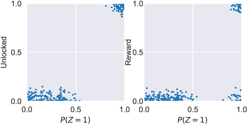
Figure 4: Scatter plot of $P(Z=1)$ and (left) chance of unlocking the door, and (right) chance of successfully reaching the goal state. The causal variable $Z$ appears to correspond to opening the door.

We have argued that the NIE offers a novel way to define coarse-grained causal knowledge. In identifying a causal variable, our method learns a policy to manipulate it, and the variables are learned directly from experience without requiring specification of a generative process. We have shown the conditional expectations involved can be estimated using an $n$-step temporal difference methods, and that the method has convergence properties comparable to TD learning (but with worse constants). We found that the method was able to learn a causal variable which was both sensible and relevant for solving a task, and did so better than a natural (non-causal) alternative method. An independent experiment on a test-set indicated the causal representation is associated with an increased NIE, and that the causal representation is relevant for the task in that it resulted in a performance increase.

References

- Alwin and Hauser (1975) Alwin, D. F.; and Hauser, R. M. 1975. The decomposition of effects in path analysis. American sociological review, 37–47.
- Amirinezhad, Salehkaleybar, and Hashemi (2020) Amirinezhad, A.; Salehkaleybar, S.; and Hashemi, M. 2020. Active Learning of Causal Structures with Deep Reinforcement Learning. arXiv preprint arXiv:2009.03009.
- Bacon, Harb, and Precup (2017) Bacon, P.-L.; Harb, J.; and Precup, D. 2017. The option-critic architecture. In Proceedings of the AAAI Conference on Artificial Intelligence, volume 31.
- Besserve et al. (2020) Besserve, M.; Mehrjou, A.; Sun, R.; and Schölkopf, B. 2020. Counterfactuals uncover the modular structure of deep generative models. In Eighth International Conference on Learning Representations (ICLR 2020).
- Camacho et al. (2019) Camacho, A.; Icarte, R. T.; Klassen, T. Q.; Valenzano, R. A.; and McIlraith, S. A. 2019. LTL and Beyond: Formal Languages for Reward Function Specification in Reinforcement Learning. In IJCAI, volume 19, 6065–6073.
- Dasgupta et al. (2019) Dasgupta, I.; Wang, J.; Chiappa, S.; Mitrovic, J.; Ortega, P.; Raposo, D.; Hughes, E.; Battaglia, P.; Botvinick, M.; and Kurth-Nelson, Z. 2019. Causal reasoning from meta-reinforcement learning. arXiv preprint arXiv:1901.08162.
- Davis, Shrobe, and Szolovits (1993) Davis, R.; Shrobe, H.; and Szolovits, P. 1993. What is a knowledge representation? AI magazine, 14(1): 17–17.
- Deisenroth and Rasmussen (2011) Deisenroth, M.; and Rasmussen, C. E. 2011. PILCO: A model-based and data-efficient approach to policy search. In Proceedings of the 28th International Conference on machine learning (ICML-11), 465–472. Citeseer.
- Espeholt et al. (2018) Espeholt, L.; Soyer, H.; Munos, R.; Simonyan, K.; Mnih, V.; Ward, T.; Doron, Y.; Firoiu, V.; Harley, T.; Dunning, I.; et al. 2018. Impala: Scalable distributed deep-rl with importance weighted actor-learner architectures. In International Conference on Machine Learning, 1407–1416. PMLR.
- Icarte et al. (2018) Icarte, R. T.; Klassen, T.; Valenzano, R.; and McIlraith, S. 2018. Using reward machines for high-level task specification and decomposition in reinforcement learning. In International Conference on Machine Learning, 2107–2116. PMLR.
- Lake, Salakhutdinov, and Tenenbaum (2015) Lake, B. M.; Salakhutdinov, R.; and Tenenbaum, J. B. 2015. Human-level concept learning through probabilistic program induction. Science, 350(6266): 1332–1338.
- Levine et al. (2016) Levine, S.; Finn, C.; Darrell, T.; and Abbeel, P. 2016. End-to-End Training of Deep Visuomotor Policies. J. Mach. Learn. Res., 17(1): 1334–1373.
- Lopez-Paz et al. (2017) Lopez-Paz, D.; Nishihara, R.; Chintala, S.; Scholkopf, B.; and Bottou, L. 2017. Discovering causal signals in images. In Proceedings of the IEEE Conference on Computer Vision and Pattern Recognition, 6979–6987.
- Mnih et al. (2016) Mnih, V.; Badia, A. P.; Mirza, M.; Graves, A.; Lillicrap, T.; Harley, T.; Silver, D.; and Kavukcuoglu, K. 2016. Asynchronous methods for deep reinforcement learning. In International conference on machine learning, 1928–1937. PMLR.
- Nabi, Kanki, and Shpitser (2018) Nabi, R.; Kanki, P.; and Shpitser, I. 2018. Estimation of Personalized Effects Associated With Causal Pathways. Uncertainty in artificial intelligence: proceedings of the… conference. Conference on Uncertainty in Artificial Intelligence, 2018.
- Pearl (2001) Pearl, J. 2001. Direct and indirect effects. In Proceedings of the Seventeenth conference on Uncertainty in artificial intelligence, 411–420.
- Pearl (2009) Pearl, J. 2009. Causality: Models, Reasoning and Inference. USA: Cambridge University Press, 2nd edition. ISBN 052189560X.
- Pearl (2012) Pearl, J. 2012. The mediation formula: A guide to the assessment of causal pathways in nonlinear models. Wiley Online Library.
- Pearl and Mackenzie (2018) Pearl, J.; and Mackenzie, D. 2018. The book of why: the new science of cause and effect. Basic Books.
- Pearl et al. (2009) Pearl, J.; et al. 2009. Causal inference in statistics: An overview. Statistics surveys, 3: 96–146.
- Peters, Janzing, and Schölkopf (2017) Peters, J.; Janzing, D.; and Schölkopf, B. 2017. Elements of Causal Inference - Foundations and Learning Algorithms. Adaptive Computation and Machine Learning Series. Cambridge, MA, USA: The MIT Press.
- Russell (1913) Russell, B. 1913. On the Notion of Cause’, reprinted in Mysticism and Logic and Other Essays. George Allen & Unwin.
- Schölkopf (2019) Schölkopf, B. 2019. Causality for machine learning. arXiv preprint arXiv:1911.10500.
- Shrestha and Mahmood (2019) Shrestha, A.; and Mahmood, A. 2019. Review of deep learning algorithms and architectures. IEEE Access, 7: 53040–53065.
- Spirtes et al. (2000) Spirtes, P.; Glymour, C. N.; Scheines, R.; and Heckerman, D. 2000. Causation, prediction, and search. MIT press.
- Tenenbaum et al. (2011) Tenenbaum, J. B.; Kemp, C.; Griffiths, T. L.; and Goodman, N. D. 2011. How to Grow a Mind: Statistics, Structure, and Abstraction. Science, 331(6022): 1279–1285.
- Wang, Yang, and Wang (2020) Wang, L.; Yang, Z.; and Wang, Z. 2020. Provably Efficient Causal Reinforcement Learning with Confounded Observational Data. ArXiv, abs/2006.12311.
- Zhang et al. (2019) Zhang, A.; Lipton, Z. C.; Pineda, L.; Azizzadenesheli, K.; Anandkumar, A.; Itti, L.; Pineau, J.; and Furlanello, T. 2019. Learning causal state representations of partially observable environments. arXiv preprint arXiv:1906.10437.
- Zhang and Bareinboim (2018) Zhang, J.; and Bareinboim, E. 2018. Fairness in decision-making—the causal explanation formula. In Proceedings of the… AAAI Conference on Artificial Intelligence.
- Zhang, Gong, and Schölkopf (2015) Zhang, K.; Gong, M.; and Schölkopf, B. 2015. Multi-Source Domain Adaptation: A Causal View. In AAAI, volume 1, 3150–3157.