Gaussian time-dependent variational principle for the finite-temperature anharmonic lattice dynamics

Abstract

The anharmonic lattice is a representative example of an interacting, bosonic, many-body system. The self-consistent harmonic approximation has proven versatile for the study of the equilibrium properties of anharmonic lattices. However, the study of dynamical properties therein resorts to an ansatz, whose validity has not yet been theoretically proven. Here, we apply the time-dependent variational principle, a recently emerging useful tool for studying the dynamic properties of interacting many-body systems, to the anharmonic lattice Hamiltonian at finite temperature using the Gaussian states as the variational manifold. We derive an analytic formula for the position-position correlation function and the phonon self-energy, proving the dynamical ansatz of the self-consistent harmonic approximation. We establish a fruitful connection between time-dependent variational principle and the anharmonic lattice Hamiltonian, providing insights in both fields. Our work expands the range of applicability of the time-dependent variational principle to first-principles lattice Hamiltonians and lays the groundwork for the study of dynamical properties of the anharmonic lattice using a fully variational framework.

Introduction — Variational methods form the basis of our understanding of quantum mechanical many-body systems. In a variational method, the wavefunctions or density matrices of a system are parametrized by a set of parameters whose size is much smaller than the dimension of the Hilbert space. Static and time-dependent Dirac (1930); Kramer (2008); Haegeman et al. (2011) variational methods are being actively used to study interacting many-body model Hamiltonians Haegeman et al. (2013); Ashida et al. (2018); Shi et al. (2018); Guaita et al. (2019); Rivera et al. (2019); Vanderstraeten et al. (2019a, b); Shi et al. (2020); Wang et al. (2020); Hackl et al. (2020).

The anharmonic lattice is a representative example of an interacting bosonic many-body system in materials science. The self-consistent harmonic approximation (SCHA) is a variational method for approximately finding the ground or thermal equilibrium state of an anharmonic lattice Hamiltonian Hooton (1955); Errea et al. (2011). Recently, a stochastic implementation of SCHA Errea et al. (2013, 2014); Bianco et al. (2017); Monacelli et al. (2018) was developed and attracted considerable attention. SCHA has been successfully applied to study structural phase transitions Bianco et al. (2017); Monacelli et al. (2018); Bianco et al. (2018); Aseginolaza et al. (2019a), superconductivity Errea et al. (2013, 2015, 2016); Borinaga et al. (2017); Errea et al. (2020), and charge density waves Leroux et al. (2015); Bianco et al. (2019); Zhou et al. (2020); Bianco et al. (2020); Sky Zhou et al. (2020); Diego et al. (2021), as well as to the dynamical properties such as the phonon spectral function Paulatto et al. (2015); Bianco et al. (2018); Aseginolaza et al. (2019a, b, 2020) and infrared and Raman spectra Monacelli et al. (2021).

However, SCHA is limited in that one needs to resort to a specific ansatz to study the dynamical properties. It is known that the SCHA ansatz for the position-position Green function is correct in the static limit of zero frequency and the perturbative limit of weak anharmonicity Bianco et al. (2017). However, the validity of the SCHA ansatz in the nonperturbative and dynamic regime Bianco et al. (2018); Aseginolaza et al. (2019a, b); Monacelli et al. (2021), where the dynamical theory is most necessary, has not been theoretically justified.

In this Letter, we solve this important problem by applying the time-dependent variational principle (TDVP) with Gaussian variational states Weedbrook et al. (2012); Adesso et al. (2014); Guaita et al. (2019); Hackl et al. (2020) to the anharmonic lattice Hamiltonian at finite temperature. Gaussian TDVP expands the static variational states of SCHA to states with nonzero momenta. We use the linearized time evolution to derive the position-position correlation function and prove the SCHA dynamical ansatz. We illustrate that the Gaussian TDVP is successful in describing the dynamics because it includes the 2-phonon states as true dynamical excitations. Our work connects the TDVP theory, whose application was mostly focused on model Hamiltonians for cold atoms, with anharmonic lattice dynamics and the SCHA method. Such connection gives fruitful results on both sides. In TDVP theory, the linearized time evolution and the projected Hamiltonian method Haegeman et al. (2013); Shi et al. (2018); Vanderstraeten et al. (2019a) are two different ways to compute the excitation spectrum, whose superiority over the other varies across systems Haegeman et al. (2013); Guaita et al. (2019); Hackl et al. (2020). We use the anharmonic lattice model to show that only the linearized time evolution gives correct excitation energies in the perturbative limit. On the SCHA side, we illustrate ways to systematically expand the SCHA theory by leveraging recent developments of non-Gaussian TDVP Shi et al. (2018); Wang et al. (2020); Shi et al. (2020).

Self-consistent harmonic approximation — We briefly review the key results of SCHA. Within the adiabatic Born-Oppenheimer approximation, the anharmonic lattice Hamiltonian is

$$\hat{H}=\sum_{a=1}^{N}\frac{{\hat{\widetilde{p}}}^{2}_{a}}{2M_{a}}+{\widetilde{V}}({\hat{\widetilde{r}}}_{1},...,{\hat{\widetilde{r}}}_{N}).$$ (1)

Here, $a$ is the combined index for atoms and Cartesian directions, $N=N_{\rm atm}\times d$ with $N_{\rm atm}$ and $d$ the numbers of the atoms and the spatial dimensions, respectively, $M_{a}$ the atomic mass, ${\hat{\widetilde{r}}}_{a}$ and ${\hat{\widetilde{p}}}_{a}$ the position and momentum operators, and ${\widetilde{V}}$ the Born-Oppenheimer potential energy. We set $\hbar=1$.

In SCHA, the true thermal equilibrium state of the anharmonic Hamiltonian is approximated by that of a harmonic Hamiltonian ${\hat{H}}^{\rm(H)}$:

$${\hat{H}}^{\rm(H)}=\sum_{a=1}^{N}\frac{{\hat{\widetilde{p}}}^{2}_{a}}{2M_{a}}+\widetilde{V}^{\rm(H)}(\hat{\widetilde{\mathbf{r}}}).$$ (2)

Since we study the dynamics around the SCHA equilibrium, we assume that the optimal harmonic potential $\widetilde{V}^{\rm(H)}$ is already found. The SCHA density matrix is

$${\hat{\rho}}_{0}=e^{-\beta{\hat{H}}^{\rm(H)}}/\Tr e^{-\beta{\hat{H}}^{\rm(H)}},$$ (3)

where $\beta=1/k_{\rm B}T$ is the inverse temperature. For later use, we define $\expectationvalue{\hat{A}}_{0}\equiv\Tr({\hat{\rho}}_{0}\hat{A})$.

Hereafter, we use the normal-mode representation, where the SCHA harmonic Hamiltonian becomes

$${\hat{H}}^{\rm(H)}=\sum_{m=1}^{N}\frac{\omega_{m}}{2}({\hat{p}}_{m}^{2}+{\hat{r}}_{m}^{2}),$$ (4)

with $\omega_{m}$ the eigenvalue of the SCHA dynamical matrix, and ${\hat{r}}_{m}$ and ${\hat{p}}_{m}$ the normal-mode position and momentum operators. The anharmonic Hamiltonian [Eq. (1)] can be written as

$$\hat{H}=\sum_{m=1}^{N}\frac{\omega_{m}}{2}{\hat{p}}_{m}^{2}+V(\bm{\mathbf{{\hat{r}}}}),$$ (5)

with $V(\bm{\mathbf{{\hat{r}}}})=\widetilde{V}(\bm{\mathbf{{\hat{\widetilde{r}}}}})$ the potential energy in the normal-mode representation.

In the normal-mode representation, the SCHA self-consistency equations Bianco et al. (2017) become

$$\expectationvalue{\frac{\partial{{\hat{V}}}}{\partial{r_{m}}}}_{0}=0,\quad\expectationvalue{\frac{\partial^{2}{{\hat{V}}}}{\partial{r_{m}}\partial{r_{n}}}}_{0}=\omega_{m}\delta_{m,n}.$$ (6)

Also, since ${\hat{\rho}}_{0}$ is a thermal state, we find

$$\expectationvalue{{\hat{p}}_{m}}_{0}=0,\quad\expectationvalue{{\hat{p}}_{m}{\hat{p}}_{n}}_{0}=\left(n_{m}+\frac{1}{2}\right)\delta_{m,n},$$ (7)

with $n_{m}=1/(e^{\beta\omega_{m}}-1)$ the occupation number.

Gaussian time-dependent variational principle — Next, we discuss the general principles of Gaussian TDVP for a multimode bosonic system at finite temperature. We use the set of states obtained by applying a Gaussian unitary transformation ${\hat{U}}({\bm{\mathbf{x}}})$ to the SCHA density matrix as the variational manifold:

$${\hat{\rho}}({\bm{\mathbf{x}}})={\hat{U}}({\bm{\mathbf{x}}}){\hat{\rho}}_{0}{\hat{U}^{\dagger}}({\bm{\mathbf{x}}}).$$ (8)

Here, ${\bm{\mathbf{x}}}$ is a real-valued vector that encodes all the variational parameters. We parametrize the Gaussian transformation as

$$\hat{U}({\bm{\mathbf{x}}})=\hat{D}(\bm{\mathbf{\alpha}})\hat{S}(\bm{\mathbf{\beta}},\bm{\mathbf{\gamma}}),$$ (9)

where $\hat{D}$ and $\hat{S}$ are the displacement and squeezing operators, respectively:

$$\hat{D}(\bm{\mathbf{\alpha}})= \exp(\frac{1}{\sqrt{2}}\sum_{m}(\alpha_{m}{\hat{a}^{\dagger}}_{m}-\alpha_{m}^{*}{\hat{a}}_{m})),$$ (10)

$$\hat{S}(\bm{\mathbf{\beta}},\bm{\mathbf{\gamma}})={\rm exp}\Bigg{[} \sum_{\begin{subarray}{c}m,n\\ m\leq n\end{subarray}}b_{mn}(\beta_{mn}{\hat{a}^{\dagger}}_{m}{\hat{a}^{\dagger}}_{n}-\beta_{mn}^{*}{\hat{a}}_{m}{\hat{a}}_{n})$$

$$+ \sum_{\begin{subarray}{c}m,n\\ m<n\end{subarray}}c_{mn}(\gamma_{mn}^{*}{\hat{a}^{\dagger}}_{m}{\hat{a}}_{n}-\gamma_{mn}{\hat{a}^{\dagger}}_{n}{\hat{a}}_{m})\Bigg{]},$$ (11)

where

$$b_{mn}\equiv\begin{cases}1/\sqrt{4(n_{m}+n_{n}+1)}&\text{if }m=n\\ 1/\sqrt{2(n_{m}+n_{n}+1)}&\text{if }m\neq n\end{cases},$$ (12)

$$c_{mn}\equiv 1/\sqrt{2(n_{m}-n_{n})}.$$ (13)

The variational parameters $\alpha_{m}$, $\beta_{mn}$, and $\gamma_{mn}$ are complex numbers. The parameter $\beta_{mn}$ ($\gamma_{mn}$) is defined only for $m\leq n$ ($m<n$). Here, we assume for simplicity that $\omega_{m}$’s are nondegenerate and satisfy $\omega_{1}<\omega_{2}<\cdots<\omega_{N}$. The total number of complex variational parameters is $N^{2}+N$. In the linear response regime, degeneracy does not pose any theoretical difficulty: if modes $m$ and $n$ are degenerate, one just needs to exclude $\gamma_{mn}$ from the set of variational parameters. This exclusion is done because the infinitesimal transformation parametrized by $\gamma_{mn}$ does not change ${\hat{\rho}}_{0}$ Note (1).

Each group of parameters describes a different type of excitation. Parameters $\bm{\mathbf{\alpha}}$, $\bm{\mathbf{\beta}}$, and $\bm{\mathbf{\gamma}}$ correspond to 1-phonon excitations, 2-phonon excitations with two creations or two annihilations of phonons, and 2-phonon excitations with one creation and one annihilation, respectively.

The imaginary parts of the parameters generate dynamics. For example, $\imaginary\bm{\mathbf{\alpha}}$ generates a finite atomic momentum through the displacement operator. The SCHA theory does not contain these imaginary parameters because the variational states are limited to the thermal state of a harmonic Hamiltonian. In contrast, Gaussian TDVP, which allows both the real and imaginary parts of the variational parameters to vary, naturally allows one to study the dynamics.

We define ${\bm{\mathbf{x}}}$, the vector of variational parameters as

$${\bm{\mathbf{x}}}=(\real\bm{\mathbf{\alpha}}\ \imaginary\bm{\mathbf{\alpha}}\ \real\bm{\mathbf{\beta}}\ \imaginary\bm{\mathbf{\beta}}\ \real\bm{\mathbf{\gamma}}\ \imaginary\bm{\mathbf{\gamma}})^{\intercal}.$$ (14)

Since ${\hat{\rho}}({\bm{\mathbf{x}}}=0)={\hat{\rho}}_{0}$ is the variational solution that minimizes the SCHA free energy, ${\bm{\mathbf{x}}}=0$ is a stationary point of the variational time evolution Note (1).

To apply TDVP to mixed states, we map the variational density matrices to wavefunctions by purification Nielsen and Chuang (2000); Shi et al. (2020). For each physical state in the number basis, we add an auxiliary state so that the purified wavefunction becomes

$$\ket{\Psi({\bm{\mathbf{x}}})}=[{\hat{U}}({\bm{\mathbf{x}}})\sqrt{{\hat{\rho}}_{0}}\otimes{\mathbb{1}}]\ket{\Phi^{+}},$$ (15)

where $\otimes$ denotes a tensor product, and $\ket{\Phi^{+}}$ is a maximally entangled state Nielsen and Chuang (2000) between the physical and the auxiliary modes [see Eq. (LABEL:eq:s_tdvp_Phi_def) and related discussions]. For the purified wavefunction, the expectation value of a physical operator $\hat{A}_{0}$ is

$$A(\bm{\mathbf{x}})\equiv\matrixelement{\Psi(\bm{\mathbf{x}})}{\hat{A}_{0}\otimes{\mathbb{1}}}{\Psi(\bm{\mathbf{x}})}=\expectationvalue{\hat{A}(\bm{\mathbf{x}})}_{0},$$ (16)

where

$$\hat{A}({\bm{\mathbf{x}}})={\hat{U}^{\dagger}}({\bm{\mathbf{x}}})\hat{A}_{0}{\hat{U}}({\bm{\mathbf{x}}}).$$ (17)

The variational time evolution is obtained by projecting the true dynamics of the wavefunction to the tangent space of the variational manifold. The tangent space is spanned by the tangent vectors, which at ${\bm{\mathbf{x}}}=0$ are

$$\ket{V_{\mu}}= \left[(\partial_{\mu}{\hat{U}})\sqrt{{\hat{\rho}}_{0}}\otimes{\mathbb{1}}\right]\ket{\Phi^{+}}.$$ (18)

Using the variational linear response theory Hackl et al. (2020); Note (1), one can show that the retarded correlation function $G_{AB}^{\rm(R)}(\omega)$ between operators $\hat{A}$ and $\hat{B}$ is

$$G_{AB}^{\rm(R)}(\omega)=\lim_{\eta\rightarrow 0^{+}}-i(\partial_{\mu}B)\mathcal{G}^{\mu}_{{\hphantom{\mu}}\nu}(\omega+i\eta)(\Omega^{\nu\rho}\partial_{\rho}A).$$ (19)

Here, the matrix Green function $\bm{\mathbf{\mathcal{G}}}^{({})}(z)$ is defined as

$$(z-i\bm{\mathbf{K}})\bm{\mathbf{\mathcal{G}}}^{({})}(z)={\mathbb{1}},$$ (20)

where $\bm{\mathbf{K}}$ is the linearized time-evolution generator defined as

$$K^{\mu}_{{\hphantom{\mu}}\nu}=-\Omega^{\mu\rho}\partial_{\rho}\partial_{\nu}E,$$ (21)

with $E({\bm{\mathbf{x}}})=\Tr[{\hat{\rho}}(\bm{\mathbf{x}}){\hat{H}}]$. The symplectic form $\bm{\mathbf{\Omega}}$ is defined by

$$\Omega^{\mu\rho}\imaginary\innerproduct{V_{\rho}}{V_{\nu}}=\frac{1}{2}\delta^{\mu}_{{\hphantom{\mu}}\nu}.$$ (22)

By computing $\bm{\mathbf{K}}$ and the corresponding matrix Green function $\bm{\mathbf{\mathcal{G}}}^{({})}(z)$, one can find the physical correlation function $G_{AB}^{\rm(R)}(\omega)$ using Eq. (19).

Anharmonic lattice dynamics — Now, we study the dynamical properties of the anharmonic lattice Hamiltonian using Gaussian TDVP. First, the symplectic form is Note (1)

$$\bm{\mathbf{\Omega}}=\begin{pmatrix}0&-{\mathbb{1}}\\ {\mathbb{1}}&0\end{pmatrix}\oplus\begin{pmatrix}0&-{\mathbb{1}}\\ {\mathbb{1}}&0\end{pmatrix}\oplus\begin{pmatrix}0&-{\mathbb{1}}\\ {\mathbb{1}}&0\end{pmatrix},$$ (23)

with $\oplus$ the direct sum.

The three matrices correspond to the subspace spanned by the tangent vectors for the variation of $\bm{\mathbf{\alpha}}$, $\bm{\mathbf{\beta}}$, and $\bm{\mathbf{\gamma}}$, respectively. In each matrix, the bases for the first (second) block of rows and columns are the tangent vectors for the real (imaginary) parts of the parameters.

For later use, we define ${\bm{\mathbf{P}}_{1}}$, $\mathbf{P}_{2+}$, and $\mathbf{P}_{2-}$ as the projection operators to the bases of each of the three matrices. The subscripts $1$, $2+$, and $2-$ indicate the nature of the tangent vectors: 1-phonon excitations, 2-phonon excitations with two creations or two annihilations, and 2-phonon excitations with one creation and one annihilation. We also define the projection to the whole 2-phonon sector: ${\bm{\mathbf{P}}_{2}}=\mathbf{P}_{2+}+\mathbf{P}_{2-}$.

Evaluating Eq. (21), we find that the time evolution generator $\bm{\mathbf{K}}$ is the sum of the non-interacting part, 3-phonon interaction, and 4-phonon interaction (see Sec. LABEL:sec:supp_der_2 of the Supplementary Material Note (1)):

$$i\bm{\mathbf{K}}=\bm{\mathbf{H}}^{(0)}+\bm{\mathbf{V}}^{(3)}+\bm{\mathbf{V}}^{(4)},$$ (24)

where

$$\bm{\mathbf{H}}^{(0)}=\begin{pmatrix}0&i\bm{\mathbf{\omega}}\\ -i\bm{\mathbf{\omega}}&0\end{pmatrix}\oplus\begin{pmatrix}0&i{\bm{\mathbf{\omega}}}_{+}\\ -i{\bm{\mathbf{\omega}}}_{+}&0\end{pmatrix}\oplus\begin{pmatrix}0&i{\bm{\mathbf{\omega}}}_{-}\\ -i{\bm{\mathbf{\omega}}}_{-}&0\end{pmatrix},$$ (25)

$$\bm{\mathbf{V}}^{(3)}=\begin{pmatrix}0&0&0&0&0&0\\ 0&0&-i\bm{\mathbf{\Phi}}^{(3)}B&0&-i\bm{\mathbf{\Phi}}^{(3)}C&0\\ 0&0&0&0&0&0\\ -iB\bm{\mathbf{\Phi}}^{(3)}&0&0&0&0&0\\ 0&0&0&0&0&0\\ -iC\bm{\mathbf{\Phi}}^{(3)}&0&0&0&0&0\end{pmatrix},$$ (26)

$$\bm{\mathbf{V}}^{(4)}=\begin{pmatrix}0&0\\ 0&0\end{pmatrix}\oplus\begin{pmatrix}0&0&0&0\\ -iB\bm{\mathbf{\Phi}}^{(4)}B&0&-iB\bm{\mathbf{\Phi}}^{(4)}C&0\\ 0&0&0&0\\ -iC\bm{\mathbf{\Phi}}^{(4)}B&0&-iC\bm{\mathbf{\Phi}}^{(4)}C&0\end{pmatrix}.$$ (27)

Here, we defined the diagonal matrices:

$$\bm{\mathbf{\omega}}_{m,n}=\omega_{m}\delta_{m,n},$$ (28)

$$[{\bm{\mathbf{\omega}}}_{\pm}]_{mn,pq}=(\omega_{m}\pm\omega_{n})\delta_{mn,pq},$$ (29)

$$B_{mn,pq}= b_{mn}(n_{m}+n_{n}+1)\delta_{mn,pq},$$ (30)

$$C_{mn,pq}= -c_{mn}(n_{m}-n_{n})\delta_{mn,pq}.$$ (31)

The implicit summation over a pair of mode indices $m$ and $n$ implies the constraint $m\leq n$ unless otherwise noted. We also defined the anharmonicity tensor

$$\Phi^{(m)}_{n_{1},\cdots,n_{m}}=\expectationvalue{\frac{\partial^{m}V}{\partial r_{n_{1}}\cdots\partial r_{n_{m}}}}_{0}.$$ (32)

The non-interacting part $\bm{\mathbf{H}}^{(0)}$ describes the free evolution of 1- and 2-phonon excitations in the SCHA Hamiltonian. The 3-phonon interaction $\bm{\mathbf{V}}^{(3)}$ couples the 1- and 2-phonon excitations. The 4-phonon interaction $\bm{\mathbf{V}}^{(4)}$ couples the 2-phonon excitations to each other.

Finally, we study the linear response of the anharmonic lattice and compute the position-position correlation function. First, we define the non-interacting Green function $\bm{\mathbf{\mathcal{G}}}^{({0})}$:

$$(z-{\bm{\mathbf{H}}^{(0)}})\bm{\mathbf{\mathcal{G}}}^{({0})}(z)={\mathbb{1}}.$$ (33)

From Eq. (25), one finds

$$\bm{\mathbf{\mathcal{G}}}^{({0})}(z)=\bm{\mathbf{\mathcal{G}}}^{({0})}_{1}(z)\oplus\bm{\mathbf{\mathcal{G}}}^{({0})}_{2+}(z)\oplus\bm{\mathbf{\mathcal{G}}}^{({0})}_{2-}(z)$$

where

$$\bm{\mathbf{\mathcal{G}}}^{({0})}_{1}(z)=\frac{1}{z^{2}-{\bm{\mathbf{\omega}}}^{2}}\begin{pmatrix}z&i{\bm{\mathbf{\omega}}}\\ -i{\bm{\mathbf{\omega}}}&z\end{pmatrix},$$ (34)

and

$$\bm{\mathbf{\mathcal{G}}}^{({0})}_{2\pm}(z)=\frac{1}{z^{2}-{\bm{\mathbf{\omega}}}_{\pm}^{2}}\begin{pmatrix}z&i{\bm{\mathbf{\omega}}}_{\pm}\\ -i{\bm{\mathbf{\omega}}}_{\pm}&z\end{pmatrix}.$$ (35)

Next, we include the 4-phonon interaction $\bm{\mathbf{V}}^{(4)}$. We define the partially interacting Green function $\bm{\mathbf{\mathcal{G}}}^{({4})}(z)$:

$$(z-\bm{\mathbf{H}}^{(0)}-\bm{\mathbf{V}}^{(4)})\bm{\mathbf{\mathcal{G}}}^{({4})}(z)={\mathbb{1}}.$$ (36)

Since the 4-phonon interaction $\bm{\mathbf{V}}^{(4)}$ does not act on the 1-phonon sector, we find

$${\bm{\mathbf{P}}_{1}}\bm{\mathbf{\mathcal{G}}}^{({4})}{\bm{\mathbf{P}}_{1}}=\bm{\mathbf{\mathcal{G}}}^{({0})}_{1}\oplus 0.$$ (37)

For the 2-phonon sector, we obtain the Dyson equation

$${\bm{\mathbf{P}}_{2}}\bm{\mathbf{\mathcal{G}}}^{({4})}{\bm{\mathbf{P}}_{2}}={\bm{\mathbf{P}}_{2}}\bm{\mathbf{\mathcal{G}}}^{({0})}{\bm{\mathbf{P}}_{2}}+{\bm{\mathbf{P}}_{2}}\bm{\mathbf{\mathcal{G}}}^{({4})}{\bm{\mathbf{V}}^{(4)}}\bm{\mathbf{\mathcal{G}}}^{({0})}{\bm{\mathbf{P}}_{2}}.$$ (38)

Finally, we study the fully interacting Green function $\bm{\mathbf{\mathcal{G}}}^{({})}(z)$ by including the 3-phonon interaction ${\bm{\mathbf{V}}^{(3)}}$. From the definitions of $\bm{\mathbf{\mathcal{G}}}^{({})}$ and $\bm{\mathbf{\mathcal{G}}}^{({4})}$, we obtain the Dyson equation

One can solve the Dyson equations [Eqs. (38, Gaussian time-dependent variational principle for the finite-temperature anharmonic lattice dynamics)] to find Note (1)

Here, we defined $B_{+}=B$ and $B_{-}=C$. In Eq. (Gaussian time-dependent variational principle for the finite-temperature anharmonic lattice dynamics), we omitted the direct sum of the zero matrix in the ${\bm{\mathbf{P}}_{2}}$ subspace for brevity.

From Eqs. (LABEL:eq:s_transf_op_der, LABEL:eq:s_overlap_dU_ar), one finds that the matrix elements for the position operator is nonzero only for the variation of $\real\bm{\mathbf{\alpha}}$:

$$\partial_{\mu}\bm{\mathbf{r}}=\begin{pmatrix}{\mathbb{1}}&0&0&0&0&0\end{pmatrix}^{\intercal}.$$ (39)

Then, from Eqs. (19, Gaussian time-dependent variational principle for the finite-temperature anharmonic lattice dynamics), one can derive the Dyson equation for the interacting retarded position-position correlation function Note (1):

$$\bm{\mathbf{G}}_{rr}^{\rm(R)}=\bm{\mathbf{G}}_{rr}^{\rm(R0)}+\bm{\mathbf{G}}_{rr}^{\rm(R0)}\bm{\mathbf{\Pi}}_{rr}\bm{\mathbf{G}}_{rr}^{\rm(R)}.$$ (40)

The self-energy is

$$\bm{\mathbf{\Pi}}_{rr}(z)= \bm{\mathbf{\Phi}}^{(3)}\bm{\mathbf{W}}({\mathbb{1}}-\bm{\mathbf{\Phi}}^{(4)}\bm{\mathbf{W}})^{-1}\bm{\mathbf{\Phi}}^{(3)}$$ (41)

where $\bm{\mathbf{W}}$ is a diagonal matrix defined as

$$\bm{\mathbf{W}}=\sum_{s=\pm}B_{s}\frac{\bm{\mathbf{\omega}}_{s}}{z^{2}-\bm{\mathbf{\omega}}_{s}^{2}}B_{s}.$$ (42)

By recovering the mode indices and defining

$$\chi_{mn,pq}(z)\equiv\frac{1}{2} \Big{[}\frac{(\omega_{m}+\omega_{n})(n_{m}+n_{n}+1)}{(\omega_{m}+\omega_{n})^{2}-z^{2}}$$

$$-\frac{(\omega_{m}-\omega_{n})(n_{m}-n_{n})}{(\omega_{m}-\omega_{n})^{2}-z^{2}}\Big{]}\delta_{mn,pq},$$ (43)

one can rewrite Eq. (41) in a form identical to the SCHA dynamical ansatz Note (1):

$$\bm{\mathbf{\Pi}}_{rr}(z)=\bm{\mathbf{\Phi}}^{(3)}\left(-\frac{1}{2}\bm{\mathbf{\chi}}(z)\right)\left[{\mathbb{1}}-\bm{\mathbf{\Phi}}^{(4)}\left(-\frac{1}{2}\bm{\mathbf{\chi}}(z)\right)\right]^{-1}\bm{\mathbf{\Phi}}^{(3)}.$$ (44)

In Eq. (44), the implicit summation over the mode indices is done without any constraints. Equation (44) and its derivation is the main result of this Letter. When transformed to the Cartesian representation, Eq. (44) becomes identical to the SCHA dynamical ansatz [Eq. (70) of Ref. Bianco et al., 2017]. We emphasize that we rigorously derived the phonon self-energy $\bm{\mathbf{\Pi}}_{rr}(z)$ using Gaussian TDVP. Our derivation theoretically proves the SCHA dynamical ansatz.

The physical interpretation of the self-energy formula we obtained vary significantly from that of the SCHA dynamical ansatz. In Gaussian TDVP, the 2-phonon states are true dynamical excitations. However, in SCHA, the 2-phonon states do not have their own dynamics and appear only indirectly through the position dependence of the SCHA force constants. The presence of the dynamical 2-phonon excitations is the essential reason why Gaussian TDVP can describe dynamical properties while the SCHA theory cannot.

For example, the phonon lifetime is an important dynamical property of an anharmonic lattice. In Gaussian TDVP, the 1-phonon states acquire a finite lifetime by decaying to the continuum of 2-phonon states through the 3-phonon interaction. In contrast, in SCHA, there are no continuum states to which the 1-phonon states can decay. Hence, in SCHA, the phonon lifetimes can only be described with a perturbative approximation Paulatto et al. (2015) unless one resorts to an ansatz.

Discussion — A common alternative to the linearized time evolution is the projected Hamiltonian method Haegeman et al. (2013); Shi et al. (2018); Vanderstraeten et al. (2019a). There, the Hamiltonian is projected onto the tangent space of the variational manifold. Let us consider a single-mode anharmonic oscillator at $T=0$, whose Hamiltonian is

$${\hat{H}}=\frac{\omega_{0}}{2}({\hat{p}}^{2}+{\hat{r}}^{2})+\frac{\lambda a}{6}\left({\hat{r}}^{3}-\frac{3}{2}{\hat{r}}\right)+\frac{\lambda^{2}b}{24}\left({\hat{r}}^{4}-3{\hat{r}}^{2}+\frac{3}{4}\right).$$ (45)

Here, $\lambda$ is the perturbation strength. The SCHA variational Hamiltonian is

$${\hat{H}}^{\rm(H)}=\frac{\omega_{0}}{2}({\hat{p}}^{2}+{\hat{r}}^{2}),$$ (46)

and the variational ground-state energy is $\omega_{0}/2$.

Perturbation theory	$\omega_{0}-\lambda^{2}a^{2}/12\omega_{0}+\mathcal{O}(\lambda^{4})$
Linearized time evolution	$\omega_{0}-\lambda^{2}a^{2}/12\omega_{0}+\mathcal{O}(\lambda^{4})$
Projected Hamiltonian	$\omega_{0}-\lambda^{2}a^{2}/16\omega_{0}+\mathcal{O}(\lambda^{4})$

Table 1: Excitation energy of the anharmonic oscillator [Eq. (45)] computed with three different methods.

In Table 1 we list the excitation energy, the difference of the ground- and first-excited state energy, computed using different methods Note (1). Comparing the variational methods to the perturbation theory, we find that the linearized time evolution is correct in the perturbative limit $\lambda\rightarrow 0$, while the projected Hamiltonian method is not. Since the SCHA dynamical ansatz is exact in the perturbative limit Bianco et al. (2017), this finding also holds for a general multimode anharmonic lattice at finite temperatures.

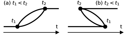
Figure 1: Diagrams of the two processes that appear in the time domain representation of a bubble diagram. Created using the feynman package Ant .

This difference occurs because the projected Hamiltonian method fails to describe the effect of virtual 3- and 4-phonon states. In Fig. 1, we show the two processes that appear in the time domain representation of the bubble diagram for the phonon self-energy. Figure 1(b) describes a process involving a 4-phonon state. Since the Gaussian projected Hamiltonian method completely neglects the 3- and 4- phonon excitations, it only includes the process described in Fig. 1(a), not that of Fig. 1(b). In contrast, in the linearized time evolution, the coupling of the 1- and 2-phonon states to virtual 3- and 4-phonon states is included by an additional term related to the derivative of the tangent vectors, which is neglected in the projected Hamiltonian method Hackl et al. (2020). Thanks to this additional term, the linearized time evolution gives the correct perturbative limit, while the projected Hamiltonian cannot.

A promising future research direction based on our study is a rigorous, systematic expansion of the SCHA method to go beyond the harmonic approximation by using non-Gaussian variational transformations Shi et al. (2018). Also, the use of mixed fermionic and bosonic variational states Shi et al. (2018); Wang et al. (2020); Shi et al. (2020) will allow the study of nontrivial electron-phonon correlation such as in phonon-mediated superconductivity or polarons in anharmonic lattices.

Recently, Monacelli and Mauri also reported a proof of the SCHA dynamical self-energy in an independent work Monacelli and Mauri (2021). While Ref. Monacelli and Mauri (2021) additionally presents a numerical algorithm to compute the correlation functions, our work focuses on the link between TDVP and SCHA. Also, while the proof for the finite-temperature case in Ref. Monacelli and Mauri (2021) is based on an analogy with the $T$=0 case, our proof uses purification to rigorously derive the finite-temperature equation of motion. The results of the two works are consistent when there is an overlap.

Conclusion — In summary, we developed a variational theory for the dynamical properties of anharmonic lattices using Gaussian TDVP, establishing a firm link between Gaussian TDVP and SCHA. We provided solid theoretical groundwork for the use of the SCHA dynamical ansatz in studying spectral properties. The presence of dynamical 2-phonon excitations in Gaussian TDVP was essential to obtain correct dynamics of the 1-phonon excitations. We compared the linearized time evolution and the projected Hamiltonian methods to find that only the former is correct in the perturbative limit. Our work establishes a useful connection between TDVP and SCHA, allowing further developments in both fields.