Compact Gauge Fields on Causal Dynamical Triangulations: a 2D case study

Abstract

We discuss the discretization of Yang-Mills theories on Dynamical Triangulations in the compact formulation, with gauge fields living on the links of the dual graph associated with the triangulation, and the numerical investigation of the minimally coupled system by Monte Carlo simulations. We provide, in particular, an explicit construction and implementation of the Markov chain moves for 2D Causal Dynamical Triangulations coupled to either $U(1)$ or $SU(2)$ gauge fields; the results of exploratory numerical simulations on a toroidal geometry are also presented for both cases. We study the critical behavior of gravity related observables, determining the associated critical indices, which turn out to be independent of the bare gauge coupling: we obtain in particular $\nu=0.496(7)$ for the critical index regulating the divergence of the correlation length of the volume profiles. Gauge observables are also investigated, including holonomies (torelons) and, for the $U(1)$ gauge theory, the winding number and the topological susceptibility. An interesting result is that the critical slowing down of the topological charge, which affects various lattice field theories in the continuum limit, seems to be strongly suppressed (i.e. by orders of magnitude) by the presence of a locally variable geometry: that may suggest possible ways for improvement also in other contexts.

I Introduction

Dynamical Triangulations represent one of the open possibilities for a solution to the quest for a self-consistent Quantum Theory of Gravity. The approach is based on the so-called asymptotic safety program ass_weinberg , which has the aim of providing a renormalized theory by finding a non-perturbative UV fixed point in the space of parameters. A possibile implementation of such program is numerical and based on the exploration, by path-integral Monte Carlo methods, of the phase diagram of the discretized theory, looking for critical points in the parameter space, which are candidate UV fixed points where continuum physics could be investigated. A standard discretization is the one based on the Regge formalism regge , where space-time configurations are represented by triangulations, i.e., collections of flat simplexes glued together according to different geometries. Promising results have been obtained, in particular, by exploring Causal Dynamical Triangulations (CDT) cdt_pioneer ; cdt_review12 ; cdt_review19 ; DynTriLor ; cdt_secondord ; cdt_secondfirst ; new_phase_chars ; cdt_newhightrans ; cdt_toroidal ; cdt_quantum_Ricci_curv ; cdt_phasestruct_toroidal ; LBseminal ; LBrunning ; cdt_higherord_toroidal ; cdt_quantum_Ricci_curv_round ; LBFEMseminal , where one enforces an additional condition of global hyperbolicity by means of a space-time foliation causconds .

The properties of Dynamical Triangulations in the presence of additional quantum fields, e.g., matter or gauge fields, has been considered various times in the past. This is interesting for at least two reasons. First, if Dynamical Triangulations eventually reveal successful in describing a continuum, renormalized theory of gravity, then lattice numerical simulations of gravity coupled to matter and gauge fields will represent the appropriate setting for the investigation of the quantum cosmological regime. Second, considering additional quantum fields could be essential even in the very process of searching for an UV fixed point, since it enlarges the coupling space and the number of candidate continuum theories.

In this paper we focus on the addition of gauge fields, either Abelian or non-Abelian. This has been considered at an analytic level in the past literature cdtgauge_anal , or numerically by considering a non-compact formulation of gauge fields cdtgauge_noncompact . Our study is devoted to a full numerical implementation based on compact gauge fields: to that purpose, after a discussion about the formulation on generic triangulations, we focus on the development of the Markov chain moves and on actual numerical simulations for a simplified two-dimensional model, in particular 2D CDT, adding to it either $U(1)$ or $SU(2)$ gauge fields by minimal coupling. One advantage of the model is that it is known to be renormalizable, so that one has the possibility to analyze how the critical behavior of the system is modified by the additional coupling.

One important aspect concerns the way the gauge symmetry is implemented in the context of Dynamical Triangulations. We adopt the point of view according to which the local gauge is fixed consistently over each simplex: in this way, elementary parallel transports, which substitute the continuum gauge connection in lattice gauge theories, are naturally associated with the links of the dual graph, i.e., links connecting adiacent symplexes, which are dual to the hypersurfaces separating them. We consider this as the most natural framework, since the choice of the local reference frame is associated, both for internal and Lorentz symmetries, with the same local object, i.e., the symplex; moreover, this is also consistent with the correct counting for the density of gauge degrees of freedom cdtgauge_noncompact .

We notice that, in the particular case of 2D triangulations, there is also an equivalent choice, frequently adopted in past studies cdtgauge_anal , which associates gauge links with the actual links of the triangulation, i.e., the edges of the triangles, and gauge transformation with the triangle vertices. However, this possibility is left open only in two dimensions, due to the fact that, in this case, the hypersurfaces delimiting a simplex are one-dimensional objects and the number of simplexes equals two times the number of vertices. Since we consider the present study as a pilot exploration in view of a generalization to a larger number of dimensions, we keep the point of view discussed above.

The paper is organized as follows. In Section II we will describe the action of Yang-Mills theory minimally coupled to gravity and how we discretize it. The set of Markov chain moves adopted in our Monte Carlo simulations is described schematically in Section III, while a detailed discussion about the detailed balance conditions is postponed to the Appendix. In Section IV we will present the results of our numerical simulations and finally, in Section V we report our conclusions.

II Minimal coupling of Yang-Mills theories to CDT

In the following, we will denote by $\mathcal{C}_{G}\big{(}\mathcal{T}\big{)}$ the space of all possible gauge field configurations on the triangulation $\mathcal{T}$, and with gauge group $G$. The action for the composite gravity-gauge system can be formally decomposed, in the minimal coupling paradigm, as $S[\Phi,\mathcal{T}]=S_{CDT}[\mathcal{T}]+S_{\text{YM}}[\Phi;\mathcal{T}]$, with $\Phi\in\mathcal{C}_{G}\big{(}\mathcal{T}\big{)}$ and where $S_{\text{YM}}$ represents the minimally coupled action of the field $\Phi$ in the backgroud $\mathcal{T}$. We now have to derive the specific form which $S_{\text{YM}}$ has to take in order to represent correctly the continuum Yang-Mills theory; as a guide to this task, we will use the analogy with the flat background case.

II.1 Yang-Mills theories on a flat lattice

In the continuum, Yang-Mills field configurations can be represented by $1$-forms $A_{\mu}$ with values in the Lie algebra of the gauge group, $\text{Lie}(G)$, while the Yang-Mills action in the Euclidean space takes the form:

$$S_{\text{YM}}=\frac{1}{4}\bigintssss\limits_{\mathcal{M}}\!d^{d}x\;F^{a}_{\mu\nu}F^{a\mu\nu},$$ (1)

with $F^{a}_{\mu\nu}=\partial_{\mu}A^{a}_{\nu}-\partial_{\nu}A^{a}_{\mu}+gf^{abc}A^{b}_{\mu}A^{c}_{\nu}$, and $A_{\mu}=A^{a}_{\mu}T^{a}$, with $T^{a}$ the generators of the Lie algebra ($a\in\{1,\dots,N^{2}-1\}$ for $SU(N)$, with the standard normalization ${\rm Tr}(T_{a}T_{b})=\delta_{ab}/2$).

This theory is usually discretized on a flat cubic lattice in terms of gauge link variables $U_{\mu}(n)$, i.e., the elementary parallel transporters, with values in the gauge group, linking adiacent sites of the lattice. The continuum action can be discretized in various different ways, the simplest one is the so-called plaquette (or Wilson) action:

$$S_{\text{YM}}\equiv-\frac{2N}{g^{2}}\sum\limits_{\Box}\Big{[}\frac{1}{N}ReTr\Pi_{\Box}-1\Big{]}\,,$$ (2)

where $\Pi_{\Box}$ is the oriented product of gauge link variables around an elementary plaquette $\Box$ of the lattice, and the sum extends over all possible plaquettes; for the $U(1)$ gauge theory, $2N/g^{2}$ is substituted by $1/g^{2}$.

II.2 Yang-Mills action coupled to CDT triangulation

The continuum version of the action of a Yang-Mills theory minimally coupled to gravity (described by the Einstein-Hilbert action) reads as follows:

$$S_{\text{YM + EH}}=\bigintssss\limits_{\mathcal{M}}\!d^{d}x\sqrt{-g}\;\left[\frac{1}{4}F^{a}_{\mu\nu}F^{a\mu\nu}+(R-2\Lambda)\right],$$ (3)

where $R$ is the scalar curvature, $\Lambda$ is the cosmological constant and the $g$ in $\sqrt{-g}$ stands in this case for the determinant of the metric tensor. In two dimensions, which is the specific case considered in this study, the Gauss-Bonnet theorem makes the curvature term only dependent on the global topology of the manifold: since the latter is usually kept fixed in CDT simulations (e.g., toroidal), such term can be ignored, leaving the cosmological constant as the only relevant coupling in the gravity sector.

Indeed, the pure-gravity action contribution for CDT in two dimensions, after Wick rotation to the Euclidean space, has the simple expression cdt_review12 :

$$S_{CDT,2D}[\mathcal{T}]=\lambda N_{2}[\mathcal{T}],$$ (4)

where $N_{2}[\mathcal{T}]$ is the number of triangles in the triangulation $\mathcal{T}$ (i.e., the total volume), and $\lambda$ is the only free parameter, which is related to the cosmological constant. When considering the path-integral formulation of pure CDT, i.e., the integral over all possible triangulations weighted by $\exp(-S_{CDT,2D}[\mathcal{T}])$, one observes a critical behavior as $\lambda\to\lambda_{c}=\log 2$ from above, where both the average global volume and the correlation length for foliation volumes diverge.

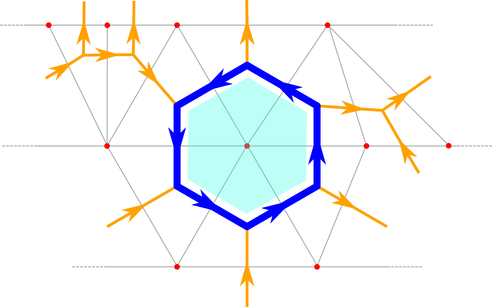
Figure 1: Sketch of a gauge plaquette on a typical 2D CDT triangulation. For simplicity, we have considered a plaquette around a vertex with zero cruvature, i.e., $n_{b}=6$. The direction of gauge links not belonging to the plaquette has been drawn according to the convention adopted in our code, i.e., from left to right and from bottom to up. Even if drawn differently, due to the representation on a plane, all triangles in this and the following figures should be considered equilateral.

Let us now consider the discretization of gauge fields. As already explained in the introductory discussion, we assume that a different choice of the local gauge is associated with each single simplex. Therefore, the information about the gauge connection is carried over by the elementary parallel transporters connecting each couple of adiacent simplexes: the gauge links connect ideally the centers of the simplexes, so they all have equal elementary length and are naturally associated with the links of the dual graph.

For a 2D causal triangulation, like that sketched in Fig. 1, one can easily describe the gauge configuration as $U_{\mu}(s)$, where $s$ stands for a particular simplex (the analogous of a lattice site in standard lattice gauge theories) and $\mu$ is either temporal or spatial, with positive orientations taken upward in time and rightward in space; each simplex is associated with two spatial links (one ingoing and one outgoing) and with just one temporal link (either ingoing or outgoing). Of course this structure is specific to causal triangulations, while the general formulation described in the previous paragraph applies to general (including non causal) triangulations.

In this formulation, the elementary gauge invariant objects are associated with traces of elementary closed loops over the dual graph: an example is shown in Fig. 1 for the 2D case. In analogy with standard lattice gauge theories, the name plaquette will be used for these elementary closed loops. A plaquette encloses an elementary two-dimensional surface of the dual graph, which is dual to a $(d-2)$ simplex of the original triangulation: this is usually known as a bone in the Regge terminology regge , and is the geometrical object where curvature resides in the Regge formulation. In the dual graph representation, it becomes the object where the gauge curvature resides as well.

A plaquette $\Pi_{b}$ centered around bone $b$ will then correspond to the ordered product of $n_{b}$ dual link variables around $b$, where $n_{b}$ is the coordination number of the bone $b$. In the particular example shown in Fig. 1, $n_{b}=6$. We remind the reader that for a two-dimensional triangulation $n_{b}=6$ corresponds to a locally flat space-time, while $n_{b}<6$ and $n_{b}>6$ correspond, respectively, to positive and negative local curvature.

The area enclosed by an elementary plaquette is $An_{b}$, where $A$ is an elementary unit of area (one third of the simplex area in two dimensions). Therefore, it is easy to write down the correspondence between plaquettes and continuum field strengths in the naïve continuum limit:

$$\Pi_{b}\simeq\exp\left(ign_{b}AF_{\mu\nu}\right)$$ (5)

where $\mu$ and $\nu$ define the directions orthogonal to the bone. When one takes the trace of the plaquette, in order to obtain a gauge invariant contribution, the second order expansion of the previous expression gives origin to the standard $F_{\mu\nu}^{2}$ contribution in the action; however this is accompained by a $n_{b}^{2}$ factor which, contrary to standard lattice gauge theories where the lattice geometry is fixed, is a dynamical variable that must be properly taken into account, as we discuss in the following.

In the continuum action, $F_{\mu\nu}^{2}$ stands in front of the $d^{d}x\sqrt{-g}$ factor, which is a measure of the physical volume. The volume can be counted over the triangulation in many different ways: one obvious way is to sum over all symplexes counting an elementary volume for each of them; an alternative way, which is useful for our purposes, is to sum over all bones $b$, taking into account that the volume around each bone is proportional to the number of simplexes sharing the same bone, i.e., to the coordination number $n_{b}$. From this reasoning, it is clear that an action which is given as a sum over bones, as the plaquette action in our case, must include a factor $n_{b}$ for each bone. Since $F_{\mu\nu}^{2}$ comes out of the plaquette with a $n_{b}^{2}$ factor attached, it is necessary to divide by $n_{b}$ the contribution from each plaquette.

To summarize, the form of the plaquette action over a triangulation $\mathcal{T}$ can be written, apart from a global factor, as follows

$$S_{\text{YM}}\equiv-\beta\!\!\!\!\sum\limits_{b\in\mathcal{T}^{(d-2)}}\!\!\frac{\widetilde{\Pi}_{b}}{n_{b}},$$ (6)

where we use the shorthand $\widetilde{\Pi}_{b}\equiv[\frac{1}{N}ReTr\Pi_{b}-1]$, the set of all bones of the triangulation $\mathcal{T}$ is denoted by $\mathcal{T}^{(d-2)}$ (which are $(d-2)$-simplexes) and $\beta$ is proportional to $1/g^{2}$. This expression is valid for any dimension $d$.

III Algorithm for 2D CDT

The Monte Carlo computation of path-integral averages in the discretized theory requires to sample the possible triangulation+gauge field configurations according to the path-integral weight $\exp(-S_{CDT,2D}-S_{\text{YM}})$, with action contributions given by Eqs. (4) and (6). This is achieved, as usual, by a set of Markov chain moves which must be properly selected in order to ensure detailed balance, ergodicity and aperiodicity. Since the action is local, a convenient set of moves is given by elementary steps that change locally the triangulation, the gauge configuration or both.

In pure gravity CDT simulations, one needs ergodic moves that modify the triangulation without spoiling the foliation, that is, the move must modify the geometry while maintaining the causal structure. A commonly used set are the Alexander moves alexander ; cdt_2dmoves , which in two dimensions are denoted by $(2,2)$, $(2,4)$ and $(4,2)$, as the number of triangles involved before and after the move: they are Metropolis–Hastings steps metro ; hastings , which respectively reorder, create or destroy a subset of simplexes and that we will review later in this section. When we consider gauge field coupled to gravity, the space of gauge configurations $\mathcal{C}_{G}\big{(}\mathcal{T}\big{)}$ depends also on the triangulation $\mathcal{T}$. The action of the Alexander moves, thus, have also an effect on the gauge field, including the creation or destruction of gauge links, that must be properly taken into account.

Moreover, we require a set of moves ensuring that the Markov chain can ergodically explore the configuration space of gauge fields $\mathcal{C}_{G}\big{(}\mathcal{T}\big{)}$ at fixed geometry, that is, by changing the gauge configuration while maintaining the triangulation invariant.

In the following, we provide a brief description of the local moves implemented in our Markov chain Monte Carlo algorithm. A more detailed discussion about detailed balance for such moves is reported in the Appendix.

III.0.1 Pure gauge move

The YM gauge move is similar to the one generally employed in lattice gauge theories with flat background. After the random selection of a link $l$ of the dual lattice, we have to extract a new value of the link variable $U_{l}^{\prime}$ from the gauge group $G$. In order to do that, we have chosen a standard heat-bath algorithm, meaning that the new link variable $U_{l}^{\prime}$ is selected according to the distribution fixed by the heat bath of nearby gauge link variables.

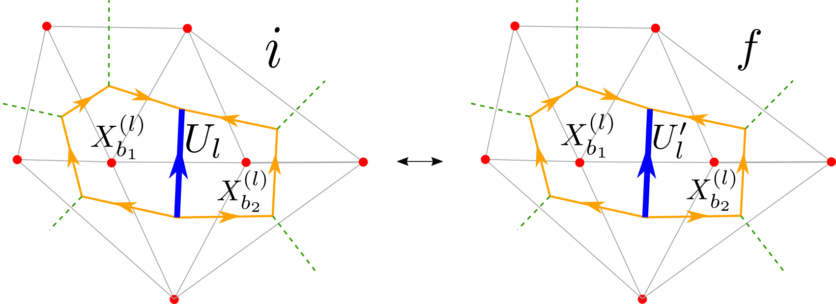
Figure 2: Sketch of a typical gauge move, where the only difference between the initial and final state is the value of the link variable associated to the edge $l$ (in blue) of the graph dual to the triangulation. The orientation of the link products for the staples $X^{(l)}_{b_{1}}$ and $X^{(l)}_{b_{2}}$ is indicated by the arrows (in the orange path).

In practice, such distribution can be expressed in terms of the local force $F_{l}\equiv\sum\limits_{b\ni l}(X_{b}^{(l)}/n_{b})$ acting on that link, where $X_{b}^{(l)}$ is the staple going around the bone $b$, i.e., the ordered product of the other links that form the plaquettes around $b$ that contains $l$, as sketched in Fig. 2. The distribution stemming from Eq. (6) is

$$P(U_{l}^{\prime})dU_{l}^{\prime}\propto dU_{l}^{\prime}\exp\left(\frac{\beta}{N}\textrm{Re Tr}\left[U_{l}^{\prime}F_{l}^{\dagger}\right]\right).$$ (7)

where $dU_{l}^{\prime}$ stands for the Haar measure over the gauge group. The distribution above is sampled using standard algorithms already employed in $U(1)$ or $SU(N)$ lattice gauge theories hb_creutz ; hb_kennedy-pendleton .

III.0.2 Triangulation move $(2,2)$

As shown in Fig. 3, the move $(2,2)$ consists in flipping a time-like edge of the triangulation and thus the associated dual link. Under such a move, the volume of the triangulation does not change and the purely gravitational part of the action remains constant. The change of the triangulation also changes the space $\mathcal{C}_{G}\big{(}\mathcal{T}\big{)}$ of the gauge configurations, however, because of the gauge freedom, this effect can be easily accounted for.

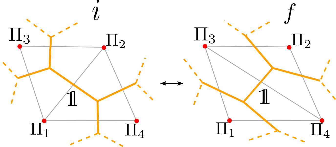
Figure 3: Sketch of a $(2,2)$ move, where the edge dual to the flipped link is gauge fixed to the identity. Notice that, even if the plaquettes involved $\Pi_{1\leq i\leq 4}$ keep the same value after the move, their contribution to the action does change because the coordination numbers of all the four involved vertices change.

Indeed, the links are not gauge invariant quantities, so in every node of the dual graph we can always perform a gauge transformation as the action of an element $g\in G$ of the group on the links that enter and exit the node. In particular, in both the initial and the final configurations we can always set the value of the central link equal to the group identity $\mathds{1}\in G$. That permits to easily identify the final gauge configuration apart from an irrelevant gauge transformation, so that a Metropolis–Hastings accept-reject step can be performed, as described in more details in the Appendix.

III.0.3 Triangulation $(2,4)$-$(4,2)$ moves

Unlike the other moves, the $(2,4)$ and $(4,2)$ ones change the volume of the triangulation, respectively creating and eliminating two triangles and a vertex of coordination four, giving a variation of the CDT part of the action equal to $\Delta S^{(2,4)}_{CDT}=-\Delta S^{(4,2)}_{CDT}=2\lambda$. The effect on the gauge configuration is thus, respectively, the introduction or the removal of a central plaquette $\Pi_{0}^{\prime}$ of length four, as we can see from Fig. 4.

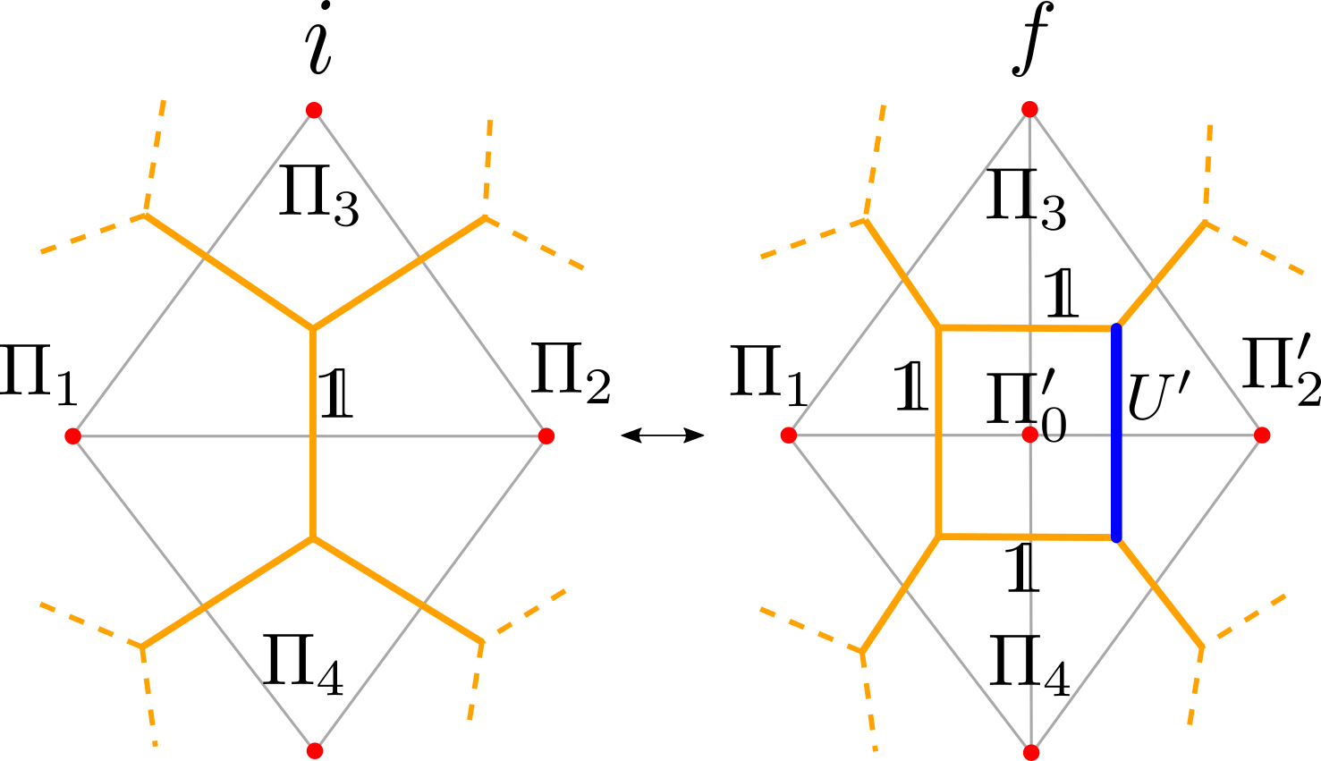
Figure 4: Sketch of a $(2,4)$ move and its inverse. The link variable $U^{\prime}$ (in blue) is the newly extracted one, as described in more details in the Appendix.

Since the plaquettes are gauge invariant observables, gauge transformations can set to the identity $\mathds{1}$ at most three out of four links of the central plaquette $\Pi_{0}^{\prime}$, shifting all the physical content in the remaining one.

Let us consider for example the $(2,4)$ move. When performing this move, the plaquette that we introduce must in general have a non-trivial value. This is necessary in order for this move to be the inverse of the $(4,2)$ one, in which the value of the destroyed $\Pi_{0}^{\prime}$ plaquette is arbitrary and not fixed by us. Therefore, the $(2,4)$ move must involve the extraction of a new link variable $U^{\prime}$, which also changes the value of the plaquette $\Pi_{2}^{\prime}$. Details on our choice for the extraction probability are reported in the Appendix.

The variation of the YM gauge action now receives a contribution both from the variation of the coordination number $n_{b}$ for the preexisting plaquettes $\Pi_{1}$, $\Pi_{3}$ and $\Pi_{4}$ and from the creation of the link variable $U^{\prime}$. The move is completed by a Metropolis–Hastings accept-reject step.

IV Numerical Results

In this Section we present and discuss the results of our numerical simulations of 2D CDT minimally coupled to Yang-Mills theories, considering either $G=U(1)$ or $G=SU(2)$ as a gauge group. We briefly recap the bare parameters entering the discretized theory: the cosmological parameter $\lambda$, defined in Eq. (4), and the inverse gauge coupling $\beta\propto 1/g^{2}$, defined in Eq. (6). We notice that the definition of $\beta$ differs from other definitions reported in the literature for discretized Yang-Mills theories by a proportionality factor, due to the explicit presence of the bone coordination numbers $n_{b}$ in the expression of the action, but also due to the fact that the reference dual lattice in the flat limit is hexagonal. In any case, nothing changes regarding the expected running of $\beta$ as the continuum limit of pure Yang-Mills is approached, i.e., $\beta\propto 1/a^{2}$ for a two-dimensional theory.

A further parameter characterizing the sampled triangulations is the number of temporal slices $N_{t}$, which is fixed, while the spatial extension of each slice is a dynamical variable and is part of the observables studied in the following. The value of $N_{t}$ has been fixed for each simulation in order to guarantee that we dealt with negligible finite size effects: this is ensured by comparing $N_{t}$ with the system correlation lengths in the temporal direction, either gravity related or gauge related, that we will define and discuss in the following. The overall imposed topology is toroidal, i.e., with periodic boundary conditions both in the temporal and spatial directions: that amounts, because of the Gauss-Bonnet theorem in two-dimensions, to globally flat geometries, meaning that we expect $\langle n_{b}\rangle=6$.

In the following we start by describing gravity related observables, which are then analyzed to sketch the phase diagram of the discretized models in the $\lambda-\beta$ plane and compare it with general expectations based on a strong coupling (i.e., small $\beta$) expansion. Then we illustrate the behavior of some gauge observables, in particular we consider the correlation function of the holonomies (torelons) and for the $U(1)$ case, the analysis of topological observables. The latter will give us illuminating hints on how a variable geometry can strongly ameliorate well known algorithmic problems like topological freezing.

IV.1 Gravity related observables

We have considered the total volume of the triangulation $V\equiv N_{2}$ (i.e., the total number of triangles) and the volume profiles, i.e., the number of spatial links (spatial edges of the triangles) $V(t)\equiv N_{1s}(t)$ in each slice, where $t$ labels the slice time. From 2d constraints, $V$ equals two times the integral of $V(t)$ and is expected to diverge at the phase transition; $V(t)$ contains more information, in particular its two-point function is expected to show a critical behavior at the phase transition, with a diverging correlation length.

The connected two-point correlation function of $V(t)$ is defined as

$$C_{\text{Vprof.}}(\Delta t)\equiv\frac{\langle V(t)V(t+\Delta t)\rangle-\langle V(t)\rangle\langle V(t+\Delta t)\rangle}{\langle V(t)^{2}\rangle-\langle V(t)\rangle^{2}},$$ (8)

with periodic conditions implied; in the actual computation we assumed $\langle V(t+\Delta t)\rangle=\langle V(t)\rangle$ and took an average over all slices. In practice, we performed a blocked resampling of the expression in Eq. (8) over many configurations, and we fitted the curve $C_{\text{Vprof.}}$ as a function of $\Delta t$ to an exponential function $\propto\exp(-\Delta t/\xi_{\text{Vprof}})$, in order to extract the correlation length of volume profiles, $\xi_{\text{Vprof}}$.

Fig. 5 shows an example of the determination of the two-point function for $\beta=0.01$ and $\lambda=0.695871$ in the $U(1)$ case. We report determinations for three different values of $N_{t}=20,60$ and 100, the correlation function is symmetric under half-lattice reflections by construction, because of the periodic boundary conditions. Finite size effects are under control in this case at least for the two largest values of $N_{t}$. Indeed, an exponential fit limited to the first half of the lattice returns $\xi_{\text{Vprof}}=5.20(2)$ for $N_{t}=60$ and $\xi_{\text{Vprof}}=5.26(2)$ for $N_{t}=100$, the reported errors include systematics related to the variation of the fit range, the reduced $\chi^{2}/{\rm dof}$ test was of $O(1)$ in all cases. A similar analysis has been performed for other simulation points.

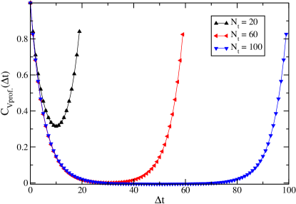
Figure 5: $2$-point connected correlation function for the volume profiles at $\beta=0.01$, $\lambda=0.695871$ and three different number of slices: $N_{t}=20,60$ and $100$.

IV.2 Phase diagram

In two dimensions, the phase diagram of pure gravity CDT presents a critical point for $\lambda_{c}=\log(2)\simeq 0.693147$ (see Refs. two_dim_scaling ; two_dim_scaling2 ; cdt_review12 ). Triangulations are weighted in the path-integral by a $\exp(-\lambda V)$ factor, so that the parameter $\lambda$ plays a role similar a chemical potential coupled do $V$: lowering the value of $\lambda$ results in an increase of $\langle V\rangle$, until it diverges as $\lambda\to\lambda_{c}$ from above. In particular, we expect the average volume to present a critical behavior which can be fitted to a power law scaling of the form:

$$f(\lambda)=\frac{A}{(\lambda-\lambda_{c})^{\mu}},$$ (9)

where $\mu$ is a critical index. The correlation length $\xi_{V_{prof}}$ is expected to follow a similar behavior, although with a different critical index $\nu$.

The effect of the introduction of the gauge coupling can be estimated in the strong coupling (low $\beta$) limit. Indeed, for $\beta\to 0$ gauge links are randomly distributed and the plaquette averages to zero. Therefore, taking into account that by the Gauss-Bonnet theorem triangulations have zero average curvature, i.e. $\langle n_{b}\rangle=6$, the typical action of a gauge configuration is expected to be approximately $\beta N_{0}/6=\beta N_{2}/12$. That can be seen as an effective shift of the $\lambda$ parameter to $\widetilde{\lambda}\simeq(\lambda+\beta/12)$, so that the critical threshold is expected to move to $\widetilde{\lambda}_{c}=\log(2)\implies\lambda_{c}^{(G)}(\beta)=\log(2)-\beta/12$.

In Fig. 6 we show results obtained for the average volume $\langle V\rangle$ and for the correlation length from simulations with gauge group $U(1)$ at $\beta=1$. A fit according to Eq. (9) works perfectly for both $\langle V\rangle$ and the correlation length, obtaining $\lambda_{c}^{(G)}=0.6068(1),\ \mu=0.357(7)$ for the former ($\chi^{2}/{\rm dof}=5.7/13$) and $\lambda_{c}^{(G)}=0.6064(2),\ \nu=0.53(3)$ for the latter ($\chi^{2}/{\rm dof}=8.6/13$): that confirms that the two quantities lead to a consistent determination of $\lambda_{c}$ (even if with a different critical index) and that the critical value is shifted below $\log 2$.

A similar analysis has been repeated for different values of $\beta$, both for $U(1)$ and $SU(2)$. In Fig. 7 we report the quantity $\log 2-\lambda_{c}^{(G)}(\beta)$ obtained in the two cases and over a wide range, comparing it with the strong coupling prediction discussed above, which seems to work perfectly until $\beta\lesssim 1$. What is more interesting is to look at the critical indices, which are reported in Fig. 8 and appear to be independent of $\beta$ in the whole range, suggesting that the only effects of the gauge fields on gravity observables consist in a shift of $\lambda_{c}$. On the basis of the apparent stability of the critical indices, we have performed a fit of all determinations to a constant value, obtaining $\mu=0.363(3)$ ($\chi^{2}/\textrm{dof}=9/9$) and $\nu=0.496(7)$ ($\chi^{2}/\textrm{dof}=9.1/9$).

One could argue that this is not unreasonable, since it is known (see, e.g., the discussion in Refs. cdtgauge_anal ; Cao:2013na ; bonati_flatsuscu1 ) that two-dimensional gauge fields can be easily integrated away: after a proper gauge fixing which freezes spatial dual gauge links, one is left with a theory of plaquettes and the path integral over them can be performed. Nevertheless, on a curved geometry one is left with a non-trivial contribution to the remaining path-integral, depending on the coordination numbers $n_{b}$: according to our numerical results, such contribution seems to be irrelevant, at least for what concerns the critical properties of the system. It is interesting to notice that the critical index of the correlation length turns out to be compatible with $1/2$ within errors, i.e. with a mean field behavior which could explain why the local fluctuations of $n_{b}$ are not relevant.

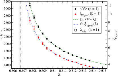
Figure 6: Determination of $\langle V\rangle$ and $\xi_{\text{Vprof.}}$ as a function of $\lambda$ for $U(1)$ at $\beta=1$. We report the results of a fit to a power law behavior as in Eq. (9) (see text).

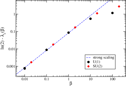
Figure 7: Critical points for the $U(1)$ and $SU(2)$ gauge theories minimally coupled to two-dimensional CDT as a function of $\beta$.

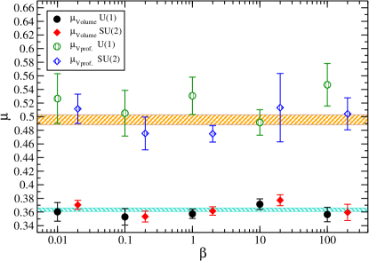
Figure 8: Critical indices $\mu$ and $\nu$ associated respectively to $\langle V\rangle$ and $\xi_{\text{Vprof.}}$ (see Eq. (9)), plotted as a function of the bare gauge coupling $\beta$. Data for the gauge groups $G=U(1)$ and $SU(2)$ have been slightly shifted horizontally to improve readability. The horizontal bands represent the results of a fit to constant values discussed in the text.

IV.3 Gauge observables

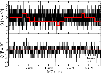
Figure 9: Comparison of topological charge histories at $\beta=60$ and $70$ for the static (flat) and dynamic simulations at average volume $N_{2}=800$.

The first gauge observable considered in our study is the topological charge, or winding number of the gauge field. It counts the winding of the gauge field at infinity and, in two-dimensions, is non-trivial only for the $U(1)$ gauge group: in this case it amounts to the total flux through the two-dimensional manifold of the field strength, which is quantized for a compact manifold like a torus or if vanishing conditions are imposed for the field strength at infinity. A possible discretization, keeping integer values as in the continuum, is the following:

$$Q\equiv\frac{1}{2\pi}\sum_{b\in\mathcal{T}^{(d-2)}}\arg[Tr(\Pi_{b})],$$ (10)

where $\Pi_{b}$ is the plaquette around the vertex $b$, and the argument produced by $\arg z$ is restricted in the interval $(-\pi,\pi]$. The cumulants of the topological charge distribution are related to the expansion of the free energy density $f$ of the gauge theory in powers of the topological parameter $\theta$. In particular the topological susceptibility, $\chi\equiv\langle Q^{2}\rangle/V$, fixes the leading order quadratic dependence, $f(\theta)=\chi\theta^{2}/2+O(\theta^{4})$.

The fact that gauge configurations relevant to the path-integral divide, in the continuum, in homotopy classes characterized by different integer values of $Q$, is at the origin of the infamous critical slowing down of topological modes in Monte Carlo simulations, also known as topological freezing, when the continuum limit is approached Alles:1996vn ; top_freeze ; Luscher:2011kk ; Bonati:2017woi : the tunneling between different topological sectors becomes more and more suppressed, as it involves the sampling of large action configurations. It is then interesting to understand what is the impact of an underlying fluctuating geometry on this problem.

There are at least two reasons to expect such an impact, and to expect that it is in the direction of an improvement: i) the creation/destruction of portions of space-time and of the gauge fields living on them may in principle enhance the tunneling events; ii) plaquettes enter the action in Eq. (6) divided by a $n_{b}$ factor, which however is not present in the topological charge in Eq. (10), so that plaquettes centered around bones with a high coordination number $n_{b}$ are possible sources of large local fluctuations of the field strength flux, with a special discount in the action.

A strong improvement in topological freezing is indeed what we observe. For the sake of comparison, we have considered also simulations of the compact $U(1)$ gauge theory on a static toroidal (i.e., flat) hexagonal lattice. Fig. 9 shows a comparison between the Monte Carlo histories of the topological charge for the static and dynamical case and for two values of $\beta$, $\beta=60$ and $70$; the comparison has been made for an equivalent total volume, namely $V=800$ for the static flat lattice and $\lambda$ tuned so as to fix $\langle V\rangle\simeq 800$ for the dynamical one, with $N_{t}=20$ in both cases. The emergence of topological freezing is quite clear in static simulations and $Q$ is completely frozen for $\beta=70$: on the contrary, this is not observed in dynamical simulations and not even for higher values of $\beta$. Autocorrelation times of $Q$ are shown as a function of $\beta$ in Fig. 10: the increase is at least exponential in the static case and becomes prohibitive for $\beta\gtrsim 50$, while it is orders of magnitudes smaller and at most exponential in the dynamical case.

In order to better understand the origin of such improvement and differentiate between the two possible hypotheses exposed above, we have performed the following experiment. We have considered the dynamical simulation at $\beta=70$ and we have stopped updating the geometry from a certain step on, i.e., we have continued the Markov chain performing only pure gauge moves on a fixed, but non-flat, triangulation. In this way the possible improvement coming from a non-constant geometry stops, while the possible improvement coming from a non-uniform geometry, i.e. from a space-time lattice with a locally variable curvature, remains. The result of the experiment is shown in Fig. 11, which clearly demonstrates that most of the improvement comes from the non-flatness of the geometry. From an intuitive perspective, vertices with a large negative curvature (large $n_{b}$) represents large holes in the lattice where fluctuations can happen more easily leading to tunneling events between topological sectors. Such a dramatic improvement in the autocorrelation times of $Q$ could be useful also in standard simulations of lattice gauge theories, where temporary fluctuations of the underlying geometry could be considered as a way to speed up the updating of topological modes.

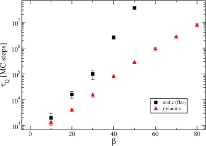
Figure 10: Comparison in topological charge autocorrelation times for the static (flat) and dynamic simulations with gauge group $U(1)$ at average volume $\langle N_{2}\rangle=800$. Measures with higher autocorrelation times than the ones shown have been dropped due to not enough statistics or to algorithmic freezing.

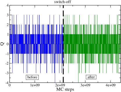
Figure 11: History of the topological charge for a simulation with gauge group $U(1)$ coupled to (dynamical) two-dimensional CDT at $\beta=70$ where we switched off all geometry updates at a certain Monte Carlo step (dashed line), after which the volume does not change ($V=800$).

Fig. 12 shows a comparison between the topological susceptibilities (times $\beta$) measured from the same simulations for the flat static and dynamical case; in the dynamical case the susceptibility has been defined as $\chi_{Q}\equiv\langle\frac{Q^{2}}{V}\rangle$, i.e., the volume fluctuations have been taken into account as well, given that, unlike the static case, $\langle V\rangle=800$ only on average in this case. The susceptibilities determined in the dynamical case slightly differ from those obtained in the static case, pointing out to an influence of the gravity coupling on gauge observables. However, in the dynamical case it is possible to obtain precise data at relatively large values of $\beta$, thus permitting a sort of (wrong) continuum limit at fixed bare gravity coupling, which, assuming $1/\beta$ corrections and considering only data with $\beta>30$, turns out to be $\beta\chi_{Q}=0.0758(14)$ with a reduced chi-squared $\chi^{2}/\textrm{dof}=1.6/3$: this is in agreement with the analytical prediction for the flat continuum theory bonati_flatsuscu1 , which, taking into account the additional factor 6 in our definition of $\beta$, is $\beta\chi_{Q}=3/(4\pi^{2})$.

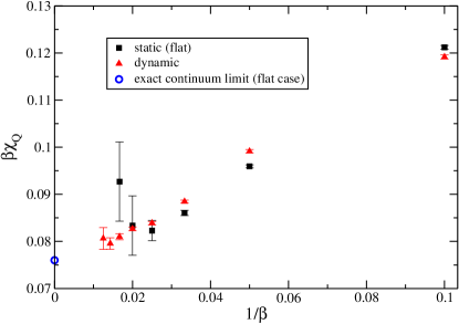
Figure 12: Comparison in topological susceptibilities for the static (flat) and dynamic simulations at average volume $N_{2}=800$.

What we have considered above has been correctly defined as a wrong continuum limit. Indeed, in order to obtain a correct continuum limit one should ensure that all correlation lengths, both gravity and gauge related, diverge; in the previous analysis, instead, we have considered either the $\lambda\to\lambda_{c}$ limit at fixed $\beta$, or the $\beta\to\infty$ limit at fixed average volume. A proper continuum limit will be obtained moving along particular curves $\lambda(\beta)$ in the $\lambda-\beta$ plane, the so-called lines of constant physics, along which the ratios of different correlation lengths is kept fixed while all of them diverge as $\beta\to\infty$. Each line of constant physics, corresponding to different ratios of correlation lengths, will define a different renormalized quantum theory.

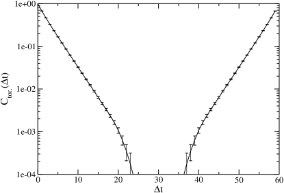
Figure 13: Connected two-point correlation function of torelon profiles for a simulation at $\lambda=-0.44244$ and $\beta=90$.

In order to go ahead with this program one should consider a set of different correlation lengths, both gravity and gauge related, in order to perform a consistent analysis. While we plan to do that more systematically in future studies, we have considered, as a first correlation length linked to the gauge field dynamics, that related to the torelon profile $\Pi(t)$, i.e. the holonomy, which is in some sense analogous to the volume profile: for a two dimensional torus triangulation we define the torelon, in analogy with the definition given on flat lattices torelons_ref1 ; torelons_ref2 , as the oriented product of link variables over the closed loop of dual-links that wraps around along a slab, that is a strip of triangles betwen two slices (labeled by $t$ as for slices); the trace of the torelon is a gauge invariant object.

As for the volume profiles, we study the connected two point correlation functions of torelonic profiles, defined as:

$$C_{\text{tor}}(\Delta t)\equiv\frac{\langle Tr\Pi(t)Tr\Pi^{\dagger}(t+\Delta t)\rangle-|\langle Tr\Pi(t)\rangle|^{2}}{\langle|Tr\Pi(t)|^{2}\rangle-|\langle Tr\Pi(t)\rangle|^{2}}\,.$$ (11)

The same considerations done for Eq. (8) apply here, and from the exponential decay of the correlator we can extract the torelon correlation length $\xi_{\text{tor.}}$.
Fig. 13 shows a typical torelonic correlation function, while in Fig. 14 we report the torelon correlation length measured for $\beta=70$ and variable $\lambda$ (above $\lambda_{c}(\beta)$). Such preliminary results show, once again, that the coupling to gravity has a non-trivial effect on gauge field dynamics, which would be interesting to better investigate in the future.

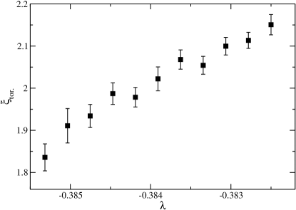
Figure 14: Torelon correlation length at $\beta=70$, as a function of the $\lambda$ parameter.

V Discussion and Conclusions

Our study has been devoted to the numerical implementation and investigation of compact gauge fields minimally coupled to Dynamical Triangulations. We have described a formulation in which local gauge transformations are associated with the elementary simplexes of the triangulation, so that the elementary gauge variables describing the gauge connection live on the links of the dual graph, which connect adiacent simplexes.

After writing an expression for the discretized plaquette action, which is reported in Eq. (6) and is valid for a generic dimension and gauge group, we have focused on two-dimensional Causal Dynamical Triangulations and on two different choices of the gauge group, either $U(1)$ or $SU(2)$. For these cases, we have developed a set of Markov chain moves for the Monte Carlo sampling of the discretized path-integral, consisting in a standard heat-bath for gauge fields at fixed triangulation plus the $(2,2)$, $(2,4)$ and $(4,2)$ moves usually adopted in 2D CDT, which have been properly modified to deal with the presence of gauge fields while preserving detailed balance (see the Appendix for a detailed discussion).

As a first numerical analysis, we have considered the critical behavior of gravity observables, in particular the total volume $V$ of the triangulation and the correlation length of the volume profile $V(t)$. In absence of the gauge fields, both are found to diverge as the cosmological coupling $\lambda$ approaches a critical value $\lambda_{c}$ from above, with $\lambda_{c}=0.69319(5)$, in agreement with the theoretical prediction $\lambda_{c}=\log 2\simeq 0.693147$. The addition of gauge fields with a finite bare gauge coupling $\beta$ has been found to modify the above scenario just for a shift in $\lambda_{c}$, which for low $\beta$ has been found to be consistent with a strong coupling estimate. In particular, the critical indices $\mu$ and $\nu$ associated with the divergence of $\langle V\rangle$ and of the correlation length are found to be independent of $\beta$ within errors, and from a fit to a constant value we have obtained $\mu=0.363(3)$ and $\nu=0.496(7)$, i.e. $\nu$ is compatible with a mean field value.

Our numerical results show also that gauge field dynamics, instead, is influenced by the coupling to gravity in a less trivial way. In this exploratory investigation we have considered just torelon correlators with the associated correlation length and, in the case of the $U(1)$ gauge group, the dependence on the topological parameter $\theta$.

An interesting observation regards a well known problem affecting the numerical simulations of standard lattice gauge theories, namely the critical slowing down of topological modes as the continuum limit is approached, also known as topological freezing. We have found, by direct comparison with simulations on a flat static lattice, that the problem is strongly reduced, by orders of magnitude in terms of the autocorrelation time, in the presence of a dynamical triangulation. Morover, we have clarified that the improvement is not linked to the dynamics of the triangulation, but just to local variations of the geometry, even at fixed triangulation: that could be due to the presence of larger holes around bones with a negative curvature, through which local topological fluctuations could happen more easily. Such observation could have interesting implications also for algorithmic developments in standard lattice gauge theories, where the local variation of the geometry could be mimicked in some way, not necessarily involving a coupling to gravity.

Future developments stemming from this exploratory study are expected in various directions. First of all, a more systematic determination of gravity related and gauge related correlation lengths will permit to fix the curves $\lambda(\beta)$ in the $\lambda-\beta$ plane along which the ratios of correlation lengths are kept fixed, i.e., the so-called lines of constant physics. Along these lines, a proper continuum limit could be taken, with all correlation lengths diverging at the same time, and with each line corresponding to a different renormalized quantum field theory. Another obvious extension is that to a larger number of dimensions, where the problem of finding a proper continuum limit is less trivial also in absence of the gauge fields, and where also the development of the set of Markov chain moves will be more challenging.

Appendix A Detailed balance for the Markov chain Monte Carlo moves

As mentioned in Section III, the path-integral probability weight for a configuration $(\mathcal{T}_{i},\Phi_{i})\in\mathcal{C}_{G}(\mathcal{T})$ of the composite gravity-gauge system can be written as:

$$P_{i}=\frac{1}{Z}e^{-S_{\text{CDT}}[\mathcal{T}_{i}]-S_{\text{YM}}[\Phi_{i};\mathcal{T}_{i}]},$$ (12)

where $Z$ is the normalization factor (partition function).

In order to ensure that the Markov chain of the Monte Carlo simulation converges to the correct equilibrium probability distribution $P_{i}$, we impose the detailed balance condition on the transition probability $W_{i\to f}$ of passing from an initial configuration $i$ to a final one $f$. Apart from the pure gauge move, in which we adopt a heat-bath algorithm, the other steps of the Markov chain are Metropolis–Hastings steps metro ; hastings , i.e., they consist in first selecting a tentative next configuration $f$ with probability $P_{\text{sel.}}(f|i)$ and then accepting it with an acceptance ratio $A_{i\to f}$. In the case in which $f$ is not accepted, the final configuration is taken to be equal to the initial one $i$. The transition probability can therefore be decomposed as the product of the selection probability and the acceptance ratio $W_{i\to f}=P_{\text{sel.}}(f|i)A_{i\to f}$ and the detailed balance condition takes the form:

$$P_{\text{sel.}}(f|i)A_{i\rightarrow f}P_{i}=P_{\text{sel.}}(i|f)A_{f\rightarrow i}P_{f}.$$ (13)

Notice that, in the general case, the selection probability cannot be controlled and we have to select the acceptance ratio in such a way as to reproduce the correct equilibrium distribution. The optimal values of the $A$s that maximize the acceptance can be found to be equal to:

$$A_{i\rightarrow f} =\min\Big{(}1,\frac{P_{\text{sel.}}(i|f)}{P_{\text{sel.}}(f|i)}\cdot\frac{P_{f}}{P_{i}}\Big{)},$$ (14a)

$$A_{f\rightarrow i} =\min\Big{(}1,\frac{P_{\text{sel.}}(f|i)}{P_{\text{sel.}}(i|f)}\cdot\frac{P_{i}}{P_{f}}\Big{)}.$$ (14b)

In this Appendix, we are going to use Eqs. (14) to derive the acceptance probabilities that satisfy the detailed balance condition for the adapted Alexander moves $(2,2)$, $(2,4)$ and $(4,2)$, that have already been schematically described in Section III. We stress that, given the complexity introduced in the moves, we have performed a series of preliminary debugging runs in which the moves have been combined with different weights, in order to check for the correctness of each single move by verifying the stability of various average observables, like the average volume or the average plaquette, against the change in the weights.

A.1 Detailed balance for the $(2,2)$ move

As this move does not change the total number of triangles, the variation of the gravitational part of the action vanishes: $\Delta S^{(2,2)}_{\text{CDT}}=0$. However, the selection probabilities of the initial and final triangulations $P_{\text{sel.},\text{CDT}}[\mathcal{T}]$ and $P_{\text{sel.},\text{CDT}}[\mathcal{T}^{\prime}]$ are in general different, giving a non trivial contribution to the acceptance: we do not review here the computation of such probabilities, which is described in standard literature on dynamical triangulations (see, e.g., Ref. cdt_review12 ).

Regarding the gauge field configuration, the gauge fixing of the central dual link variable to the group identity $\mathds{1}$ ensures that this move, involving a flip of a time-like link, does not change the values of the plaquettes but only their lengths (i.e., the coordination numbers of the associated vertices), as can be seen from Fig. 3, to which we refer in the following. Since the YM gauge action (6) depends explicitly on the plaquette lengths, its variation is non trivial:

$$\Delta S_{\text{YM}}^{(2,2)}=$$ (15)

$$\beta\Big{[}\frac{\widetilde{\Pi}_{1}}{n_{1}(n_{1}+1)}+\frac{\widetilde{\Pi}_{2}}{n_{2}(n_{2}+1)}-\frac{\widetilde{\Pi}_{3}}{n_{3}(n_{3}-1)}-\frac{\widetilde{\Pi}_{4}}{n_{4}(n_{4}-1)}\Big{]},$$

where we report the definition $\widetilde{\Pi}_{b}\equiv[\frac{1}{N}ReTr\Pi_{b}-1]$. We also stress that the selection probabilities of the initial and final gauge configuration $\Phi$ and $\Phi^{\prime}$ are trivially equal, $P_{\text{sel.},\text{YM}}[\Phi]=P_{\text{sel.},\text{YM}}[\Phi^{\prime}]$, because, given the gauge fixing, the selection procedure is deterministic in both directions.

Finally, the acceptance ratio can be found from Eqs. (14), receiving contributions both from the non-trivial ratio of the selection probabilities of the triangulations and the variation of the gauge action:

$$A^{(2,2)}=\min\Big{(}1,e^{-\Delta S_{\text{YM}}^{(2,2)}}\cdot\frac{P_{\text{sel.},\text{CDT}}[\mathcal{T}]}{P_{\text{sel.},\text{CDT}}[\mathcal{T}^{\prime}]}\Big{)}.$$ (16)

A.2 Detailed balance for moves $(2,4)$ and $(4,2)$

As we will see, this pair of moves is the most involved. To fix the ideas, let us consider the direct move $(2,4)$, which creates two new triangles, increasing the gravitational contribution to the total action: $\Delta S^{(2,4)}_{CDT}=-\Delta S^{(4,2)}_{CDT}=2\lambda$. The effect on the gauge configuration is the introduction of a new plaquette of length four, which can always be made to have all link variables but one gauge fixed to the identity $\mathds{1}$. The remaining link variable have to be extracted from the gauge group $G$ and cannot be set to the identity, since in the inverse move $(4,2)$ the plaquette which is eliminated has in general a non-trivial value, i.e., is not fixed to the identity. In the following we make reference to Fig. 4 for the notation.

Let $U^{\prime}$ denote the newly extracted link variable. The variation of the gauge action receives contributions from both the change in the lengths of the plaquettes $\Pi_{0}$, $\Pi_{3}$ and $\Pi_{4}$ and from the introduction of $U^{\prime}$:

$$\Delta S^{(2,4)}_{\text{YM}}=\beta \Big{\{}\frac{\widetilde{\Pi}_{3}}{n_{3}(n_{3}+1)}+\frac{\widetilde{\Pi}_{4}}{n_{4}(n_{4}+1)}+\frac{\widetilde{\Pi}_{2}}{n_{2}}+\frac{1}{4}-\frac{1}{n_{2}}$$

$$-\frac{1}{N}ReTr\Big{[}U^{\prime}\Big{(}\frac{\mathds{1}}{4}+\frac{X_{2}^{\dagger}}{n_{2}}\Big{)}\Big{]}\Big{\}},$$ (17)

where $X_{2}$ is the staple of $U^{\prime}$ associated with the plaquette $\Pi_{2}^{\prime}$.

There is a way to extract $U^{\prime}$ which is more convenient from the point of view of the acceptance probability: this represents a non-trivial gain, given the complexity of even trying the $(2,4)$ move or its inverse. We start noticing that, in Eq. (17), we can separate the term dependent on the new link variable $U^{\prime}$ from the one independent of it, as follows:

$$\Delta S^{(2,4)}_{YM}(U^{\prime},\{\Pi_{b}\})=\widetilde{\Delta S}^{(2,4)}_{YM}(U^{\prime},\{\Pi_{b}\})+\widehat{\Delta S}^{(2,4)}_{YM}(\{\Pi_{b}\}),$$ (18)

where we have defined:

$$\widetilde{\Delta S}^{(2,4)}_{YM}(U^{\prime},\{\Pi_{b}\})= -\frac{\beta}{N}ReTr\Big{[}U^{\prime}F^{\dagger}\Big{]},$$ (19a)

$$\widehat{\Delta S}^{(2,4)}_{YM}(\{\Pi_{b}\})= +\beta\Big{[}\frac{\widetilde{\Pi}_{3}}{n_{3}(n_{3}+1)}+\frac{\widetilde{\Pi}_{4}}{n_{4}(n_{4}+1)}$$

$$+\frac{\widetilde{\Pi}_{2}}{n_{2}}+\frac{1}{4}-\frac{1}{n_{2}}\Big{]},$$ (19b)

and the force acting on the new link variable $U^{\prime}$ is equal to $F\equiv\mathds{1}/4+X_{2}/n_{2}$.

The idea is to extract $U^{\prime}$ according to its distribution in the heat bath fixed by the force $F$, i.e., with probability distribution:

$$\frac{dU^{\prime}}{Z_{G}(F)}\exp\left(\frac{\beta}{N}\textrm{Re Tr}\left[U^{\prime}F^{\dagger}\right]\right)\,,$$ (20)

where we have written the normalization factor explicitly

$$Z_{G}(F)\equiv\bigintsss\limits_{G}dU^{\prime}\exp\left(\frac{\beta}{N}\textrm{Re Tr}\left[U^{\prime}F^{\dagger}\right]\right)\,.$$ (21)

In this way, since the initial configuration has a unique gauge equivalence class, the gauge part of the ratio of selection probabilities turns out to be exactly equal to Eq. (20), and the final Metropolis–Hastings acceptance probability gets partially simplified, in particular we obtain

$$A^{(2,4)} =\min\Big{\{}1,\frac{P_{\text{sel.},\text{CDT}}(\mathcal{T})}{P_{\text{sel.},\text{CDT}}(\mathcal{T}^{\prime})}e^{-2\lambda-\widehat{\Delta S}^{(2,4)}}Z_{G}(F)\Big{\}},$$ (22a)

$$A^{(4,2)} =\min\Big{\{}1,\frac{P_{\text{sel.},\text{CDT}}(\mathcal{T}^{\prime})}{P_{\text{sel.},\text{CDT}}(\mathcal{T})}e^{+2\lambda+\widehat{\Delta S}^{(2,4)}}/Z_{G}(F)\Big{\}}.$$ (22b)

Also in this case we do not discuss in detail the ratio of selection probabilities related to the triangulation itself, i.e., ${P_{\text{sel.},\text{CDT}}(\mathcal{T})}/{P_{\text{sel.},\text{CDT}}(\mathcal{T}^{\prime})}$, which is described in previous literature cdt_review12 .

Notice that the acceptance probability depends explicitly on the normalization factor $Z_{G}(F)$ computed as a Haar integral. As the force $F$ changes dynamically, it is necessary to compute the normalization function during the simulation. For certain groups, like $U(N)$ and $SU(N)$, an analytic expression for this integral is known Zintegral1 ; Zintegral2 . In particular, for the groups $U(1)$ and $SU(2)$ that we have studied in the numerical investigation, the normalization functions are given by:

$$Z_{U(1)}(F) =I_{0}\Big{(}2det(J)\Big{)};$$ (23)

$$Z_{SU(2)}(F) =\frac{1}{\sqrt{K(J)}}I_{1}\Big{(}2\sqrt{K(J)}\Big{)},$$ (24)

where $J\equiv\frac{1}{2g^{2}N}F$, $K(J)\equiv Tr\big{(}J^{\dagger}J\big{)}+det(J)+det(J^{\dagger})$, and we have used the modified Bessel functions of the first kind, $I_{k}$.

References

- (1) S. Weinberg, “General Relativity, an Einstein Centenary Survey”, ch.16 Cambridge Univ. Press (1979).
- (2) T. Regge, Nuovo Cim. 19 (1961), 558.
- (3) J. Ambjorn, J. Jurkiewicz and R. Loll, Phys. Rev. Lett. 85, 924-927 (2000) [arXiv:hep-th/0002050 [hep-th]].
- (4) J. Ambjorn, A. Goerlich, J. Jurkiewicz and R. Loll, Phys. Rept. 519 (2012), 127 [arXiv:1203.3591 [hep-th]].
- (5) R. Loll, Class. Quant. Grav. 37, no.1, 013002 (2020) [arXiv:1905.08669 [hep-th]].
- (6) J. Ambjorn, J. Jurkiewicz and R. Loll, Nucl. Phys. B 610, 347-382 (2001) [arXiv:hep-th/0105267 [hep-th]].
- (7) J. Ambjorn, S. Jordan, J. Jurkiewicz and R. Loll, Phys. Rev. Lett. 107, 211303 (2011) [arXiv:1108.3932 [hep-th]].
- (8) J. Ambjorn, S. Jordan, J. Jurkiewicz and R. Loll, Phys. Rev. D 85, 124044 (2012) [arXiv:1205.1229 [hep-th]].
- (9) J. Ambjørn, J. Gizbert-Studnicki, A. Görlich, J. Jurkiewicz, N. Klitgaard and R. Loll, Eur. Phys. J. C 77, no.3, 152 (2017) [arXiv:1610.05245 [hep-th]].
- (10) J. Ambjorn, D. Coumbe, J. Gizbert-Studnicki, A. Gorlich and J. Jurkiewicz, Phys. Rev. D 95, no.12, 124029 (2017) [arXiv:1704.04373 [hep-lat]].
- (11) J. Ambjørn, J. Gizbert-Studnicki, A. Görlich, K. Grosvenor and J. Jurkiewicz, Nucl. Phys. B 922, 226-246 (2017) [arXiv:1705.07653 [hep-th]].
- (12) N. Klitgaard and R. Loll, Phys. Rev. D 97, no.4, 046008 (2018) [arXiv:1712.08847 [hep-th]].
- (13) J. Ambjørn, J. Gizbert-Studnicki, A. Görlich, J. Jurkiewicz and D. Németh, JHEP 06, 111 (2018) [arXiv:1802.10434 [hep-th]].
- (14) G. Clemente and M. D’Elia, Phys. Rev. D 97, no.12, 124022 (2018) [arXiv:1804.02294 [hep-th]].
- (15) G. Clemente, M. D’Elia and A. Ferraro, Phys. Rev. D 99, no.11, 114506 (2019) [arXiv:1903.00430 [hep-th]].
- (16) J. Ambjørn, G. Czelusta, J. Gizbert-Studnicki, A. Görlich, J. Jurkiewicz and D. Németh, JHEP 05, 030 (2020) [arXiv:2002.01051 [hep-th]].
- (17) N. Klitgaard and R. Loll, [arXiv:2006.06263 [hep-th]].
- (18) F. Caceffo and G. Clemente, [arXiv:2010.07179 [hep-lat]].
- (19) E. Minguzzi and M. Sanchez, [arXiv:gr-qc/0609119 [gr-qc]].
- (20) J. Ambjorn and A. Ipsen, Phys.Rev.D 88 (2013), 6 [arXiv:1305.3148 [hep-th]].
- (21) J. Ambjorn, K. N. Anagnostopoulos and J. Jurkiewicz, JHEP 08 (1999), 016 [arXiv:hep-lat/9907027 [hep-lat]].
- (22) J.W. Alexander, Ann. Mat. 31 (1931) 292.
- (23) J. Ambjørn, J. Jurkiewicz and R. Loll, NATO Sci. Ser. C 556, 381-450 (2000) [arXiv:hep-th/0001124 [hep-th]].
- (24) N. Metropolis, A. W. Rosenbluth, M. N. Rosenbluth, A. H. Teller and E. Teller, J. Chem. Phys. 21, 1087-1092 (1953)
- (25) W. K. Hastings, Biometrika 57, 97-109 (1970)
- (26) M. Creutz, Phys. Rev. D 21, 2308-2315 (1980)
- (27) A. D. Kennedy and B. J. Pendleton, Phys. Lett. B 156, 393-399 (1985)
- (28) J. Ambjorn and R. Loll, Nucl. Phys. B 536, 407-434 (1998) [arXiv:hep-th/9805108 [hep-th]].
- (29) J. Ambjorn, R. Loll, J. L. Nielsen and J. Rolf, Chaos Solitons Fractals 10, 177-195 (1999) [arXiv:hep-th/9806241 [hep-th]].
- (30) C. Cao, M. van Caspel and A. R. Zhitnitsky, Phys. Rev. D 87, no.10, 105012 (2013) [arXiv:1301.1706 [hep-th]].
- (31) C. Bonati and P. Rossi, Phys. Rev. D 99, no.5, 054503 (2019) [arXiv:1901.09830 [hep-lat]].
- (32) B. Alles, G. Boyd, M. D’Elia, A. Di Giacomo and E. Vicari, Phys. Lett. B 389, 107-111 (1996) [arXiv:hep-lat/9607049 [hep-lat]].
- (33) L. Del Debbio, G. M. Manca and E. Vicari, Phys. Lett. B 594, 315-323 (2004) [arXiv:hep-lat/0403001 [hep-lat]].
- (34) M. Luscher and S. Schaefer, JHEP 07, 036 (2011) [arXiv:1105.4749 [hep-lat]].
- (35) C. Bonati and M. D’Elia, Phys. Rev. E 98, no.1, 013308 (2018) doi:10.1103/PhysRevE.98.013308 [arXiv:1709.10034 [hep-lat]].
- (36) C. Michael, Phys. Lett. B 232, 247-250 (1989)
- (37) E. Marinari, M. L. Paciello and B. Taglienti, Int. J. Mod. Phys. A 10, 4265-4310 (1995) [arXiv:hep-lat/9503027 [hep-lat]].
- (38) R. Brower, P. Rossi and C. I. Tan, Nucl. Phys. B 190, 699-718 (1981)
- (39) R. C. Brower, P. Rossi and C. I. Tan, Phys. Rev. D 23, 942 (1981)