One-Bit Direct Position Determination of Narrowband Gaussian Signals

Abstract

One of the main drawbacks of the well-known Direct Position Determination (DPD) method is the requirement that raw data be transferred to a common processor. It would therefore be of high practical value if DPD—or a modified version thereof—could be successfully applied to a coarsely quantized version of the raw data, thus alleviating the communication requirements between the different base stations. Motivated by the above, and inspired by recent work in the rejuvenated one-bit array processing field, we present One-Bit DPD: a direct localization method based on one-bit quantized measurements. We show that despite the coarse quantization, the proposed method nonetheless yields a position estimate with appealing asymptotic properties. We further establish the identifiability conditions of this model, which rely only on second-order statistics. Simulation results corroborate our analytical derivations, demonstrating that much of the information regarding the emitter position is preserved under this crude form of quantization.

Index Terms—  Array processing, direct position determination, emitter localization, beamforming, one-bit quantization.

1 Introduction

Emitter localization is one of the most attractive problems in signal processing, relevant to a variety of applications, such as autonomous vehicles [1, 2], radar, lidar and sonar systems [3, 4, 5], and battlefield surveillance [6], to name but a few.

Naturally, this problem has been extensively addressed in the literature and different methods have been proposed over the years. Common two-step methods are based on first estimating the signal’s Time-Of-Arrival (TOA) and / or Angle-Of-Arrival (AOA) at several base stations, and based on these estimates, the emitter position is subsequently estimated. Other methods, operating by the same principle, incorporate Frequency Difference-Of-Arrival (FDOA) estimation as well [7, 8], when possible. Since these TOA / AOA / FDOA are computed separately at each base station, they do not account for the informative constraint that all measurements from all the different base stations contain the same signal, transmitted from the underlying emitter at the unknown location.

In order to further exploit the “extra” information within this constraint, the one-step Direct Position Determination (DPD) method was proposed by Weiss in his seminal work [9], where DPD of a single emitter is addressed. Following, many variants and extensions have been proposed, e.g., [10, 11, 12, 13, 14, 15, 16, 17].

Although DPD provides higher accuracy than two-step-based alternatives, it requires the transmission of raw signal data from all base stations to a central computing unit. This entails a trade-off between localization accuracy and communication resources, which is at the heart of this paper. Our goal is thus to take one step towards a better balance with respect to (w.r.t.) this trade-off. In other words, for a prespecified desired localization accuracy, we aim to “strip” significant redundancies from the transmitted raw data.

Inspired by recent work from the flourishing field of one-bit processing (e.g., [18, 19, 20, 21, 22, 23, 24, 25]), our main contribution in this letter is One-Bit DPD (OB-DPD)—a method allowing for accurate direct localization based on quantized measurements of Gaussian signals, acquired by a $1$-bit Analog-to-Digital Converter (ADC) low-complexity receiver. In addition, we establish the respective identifiability conditions for the quantized signal model under consideration, based only on Second-Order Statistics (SOS).

2 Problem Formulation

Consider $L$ spatially diverse base stations, each equipped with an $M$-element calibrated omni-directional antenna array, and the presence of an unknown narrowband signal, emitted from a transmitter whose deterministic, unknown position is denoted by the vector of coordinates ${\mbox{\boldmath$p$}}\in\mathbb{R}^{K_{p}\times 1}$. We assume that the transmitter is sufficiently far from all $L$ base stations to allow a planar wavefront (“far-field”) approximation. The time-varying vector of sampled, baseband-converted signals from all $M$ sensors at the $\ell$-th base station array is given by

$${\mbox{\boldmath$r$}}_{\ell}[n]=b_{\ell}{\mbox{\boldmath$a$}}_{\ell}({\mbox{\boldmath$p$}})s_{\ell}[n]+{\mbox{\boldmath$v$}}_{\ell}[n]\in\mathbb{C}^{M\times 1},$$ (1)

for all time-index $n\in\{1,\ldots,N\}$, where

1. $b_{\ell}\in\mathbb{C}$ denotes the unknown channel effect (e.g., attenuation) from the transmitter to the $\ell$-th base station;

2. ${\mbox{\boldmath$a$}}_{\ell}({\mbox{\boldmath$p$}})\in\mathbb{C}^{M\times 1}$ denotes the known $\ell$-th array response to a signal transmitted from position $p$;

3. $s_{\ell}[n]\triangleq\left.s\left(t-\tau_{\ell}({\mbox{\boldmath$p$}})\right)\right|_{t=nT_{s}}\in\mathbb{C}$ denotes the unobservable sampled signal waveform at the $\ell$-th base station, where $s\left(t-\tau_{\ell}({\mbox{\boldmath$p$}})\right)$ is the analog, continuous-time waveform delayed by $\tau_{\ell}({\mbox{\boldmath$p$}})$, and $T_{s}$ is the sampling period; and

4. ${\mbox{\boldmath$v$}}_{\ell}[n]\in\mathbb{C}^{M\times 1}$ denotes the additive noise at the $\ell$-th base station, representing internal (e.g., thermal) receiver noise and “interfering” signals, modeled as spatially and temporally independent, identically distributed (i.i.d.) zero-mean circular Complex Normal (CN, [26]) vector process with a covariance matrix ${\mbox{\boldmath$R$}}_{v_{\ell}}\triangleq\mathbb{E}\left[{\mbox{\boldmath$v$}}_{\ell}[n]{\mbox{\boldmath$v$}}^{\tiny\rm{H}}_{\ell}[n]\right]=\sigma_{v_{\ell}}^{2}{\mbox{\boldmath$I$}}_{M}\in\mathbb{C}^{M\times M}$, where $\sigma_{v_{\ell}}^{2}$ is unknown, and ${\mbox{\boldmath$I$}}_{M}$ denotes the $M$-dimensional identity matrix.

We also assume that the transmitter and antenna arrays are stationary during the whole observation interval, such that no frequency shift due to the Doppler effect occurs. Further, we assume that $s(t)$ may be modeled as a stationary (not necessarily i.i.d.) zero-mean circular CN random process, statistically independent of all $\{{\mbox{\boldmath$v$}}_{\ell}[n]\}_{\ell=1}^{L}$, with an unknown auto-correlation function $R_{s}(t_{0})\triangleq\mathbb{E}\left[s(t)s^{*}(t-t_{0})\right]\in\mathbb{C}$. Consequently, we get for all $i,j\in\{1,\ldots,L\}$,

$$R^{(i,j)}_{s}[m]\triangleq\mathbb{E}\left[s_{i}[n]s_{j}^{*}[n-m]\right]=R_{s}\left(mT_{s}-\Delta_{ij}({\mbox{\boldmath$p$}})\right),$$

where $\Delta_{ij}({\mbox{\boldmath$p$}})\triangleq\tau_{i}({\mbox{\boldmath$p$}})-\tau_{j}({\mbox{\boldmath$p$}})\in\mathbb{R}$. Furthermore, it follows that $\{{\mbox{\boldmath$r$}}_{\ell}[n]\}_{\ell=1}^{L}$ are all stationary zero-mean circular CN with auto- and cross-covariance matrices (for all $i,j\in\{1,\ldots,L\}$)

$$\begin{gathered}{\mbox{\boldmath$R$}}^{(i,j)}[m]\triangleq\mathbb{E}\left[{\mbox{\boldmath$r$}}_{i}[n]{\mbox{\boldmath$r$}}^{\tiny\rm{H}}_{j}[n-m]\right]=\\ b_{i}b^{*}_{j}R^{(i,j)}_{s}[m]{\mbox{\boldmath$a$}}_{i}({\mbox{\boldmath$p$}}){\mbox{\boldmath$a$}}^{\tiny\rm{H}}_{j}({\mbox{\boldmath$p$}})+\delta_{ij}\sigma^{2}_{v_{i}}{\mbox{\boldmath$I$}}_{M}\in\mathbb{C}^{M\times M},\end{gathered}$$

where $\delta_{mn}$ denotes the Kronecker delta of $m,n\in\mathbb{Z}$. Lastly, applying the (normalized) Discrete Fourier Transform (DFT) to (1) yields the equivalent frequency-domain representation,

$$\begin{gathered}\hskip 0.34479pt\hbox to0.0pt{\leavevmode\hbox{\set@color${\mbox{\boldmath$r$}}$}\hss}{\hskip-0.34479pt\leavevmode\hbox{\set@color$\overline{\hbox{}}$}}_{\ell}[k]=b_{\ell}{\mbox{\boldmath$a$}}_{\ell}({\mbox{\boldmath$p$}})\hskip 0.39063pt\hbox to0.0pt{\leavevmode\hbox{\set@color$s$}\hss}{\hskip-0.39063pt\leavevmode\hbox{\set@color$\overline{\hbox{}}$}}[k]e^{-\jmath\omega_{k}\tau_{\ell}({\text{\boldmath$p$}})}+\hskip 0.1573pt\hbox to0.0pt{\leavevmode\hbox{\set@color${\mbox{\boldmath$v$}}$}\hss}{\hskip-0.1573pt\leavevmode\hbox{\set@color$\overline{\hbox{}}$}}_{\ell}[k]\in\mathbb{C}^{M\times 1},\\ \omega_{k}\triangleq\frac{2\pi(k-1)}{NT_{s}}\in\mathbb{R}^{+},\quad\forall k\in\{1,\ldots,N\},\end{gathered}$$

where we use $\hskip 0.20938pt\hbox to0.0pt{\leavevmode\hbox{\set@color$z$}\hss}{\hskip-0.20938pt\leavevmode\hbox{\set@color$\overline{\hbox{}}$}}[k]$ to denote the $k$-th DFT coefficient of the corresponding (discrete) time-domain signal $z[n]$ everywhere.

In this work, rather than assuming access to the discrete-time signal (1) measured by an ideal $\infty$-bit ADC, we assume access only to a “coarse” quantized version thereof, obtained by a $1$-bit ADC. Specifically, the vector of $1$-bit quantized signals from the $\ell$-th base station at time $n$ is given by

$${\mbox{\boldmath$y$}}_{\ell}[n]\triangleq\mathcal{Q}\big{(}{\mbox{\boldmath$r$}}_{\ell}[n]\big{)}\in\left\{e^{\jmath\left(\frac{\pi}{4}+\frac{\pi m}{2}\right)}:0\leq m\leq 3\right\}^{M\times 1},$$ (2)

where the complex-valued $1$-bit quantizer is defined as

$$\mathcal{Q}(z)\triangleq\frac{1}{\sqrt{2}}\cdot\Big{[}\mbox{sign}\left(\Re\{z\}\right)+\jmath\cdot\mbox{sign}\left(\Im\{z\}\right)\Big{]},\forall z\in\mathbb{C},$$ (3)

and, with slight abuse of notations, $\mathcal{Q}(\cdot)$ operates elementwise in (2). For simplicity of the exposition in some parts of the derivation which follows, we further assume that all $\{\tau_{\ell}({\mbox{\boldmath$p$}})\}$ are (at least approximately) an integer multiple of the sampling period. However, this assumption is not required in practice, and can be relaxed. This completes the definition of our model, and the problem at hand may be stated concisely as follows:

3 DPD for Non-Quantized Measurements

Since our proposed algorithm is both inspired by and closely related to the original DPD method [9], we first briefly review the DPD objective function, principal steps of the derivation, and the final closed-form expression for the estimate of $p$.

The DPD method is in fact originated by Nonlinear Least-Squares (NLS) estimation of the transmitter’s position $p$ based on the data $\{{\mbox{\boldmath$r$}}_{\ell}[n]\}$. Thus, it seeks the position estimate

$$\widehat{{\mbox{\boldmath$p$}}}_{\text{\tiny DPD}}\triangleq\underset{{\text{\boldmath$p$}}\in\mathbb{R}^{K_{p}\times 1}}{\operatorname*{argmin}}\;Q({\mbox{\boldmath$p$}}),$$

where the NLS cost function to be minimized is given by

$$Q({\mbox{\boldmath$p$}})\triangleq\min_{\begin{subarray}{c}\text{\boldmath$\bar{s}$}\in\mathbb{C}^{N\times 1}\\ {\text{\boldmath$b$}}\in\mathcal{B}_{L}\end{subarray}}\sum_{\ell=1}^{L}\left\|\hskip 0.34479pt\hbox to0.0pt{\leavevmode\hbox{\set@color${\mbox{\boldmath$r$}}$}\hss}{\hskip-0.34479pt\leavevmode\hbox{\set@color$\overline{\hbox{}}$}}_{\ell}-b_{\ell}\cdot\hskip 0.39063pt\hbox to0.0pt{\leavevmode\hbox{\set@color${\mbox{\boldmath$s$}}$}\hss}{\hskip-0.39063pt\leavevmode\hbox{\set@color$\overline{\hbox{}}$}}_{\ell}\otimes{\mbox{\boldmath$a$}}_{\ell}({\mbox{\boldmath$p$}})\right\|^{2}\in\mathbb{R}^{+},$$ (4)

$\|\cdot\|$ and $\otimes$ are the $\ell^{2}$-norm and Kronecker product, resp., $\mathcal{B}_{L}\triangleq\{{\mbox{\boldmath$z$}}\in\mathbb{C}^{L\times 1}:\|{\mbox{\boldmath$z$}}\|=1\}$, $\hskip 0.39063pt\hbox to0.0pt{\leavevmode\hbox{\set@color${\mbox{\boldmath$s$}}$}\hss}{\hskip-0.39063pt\leavevmode\hbox{\set@color$\overline{\hbox{}}$}}\triangleq\left[\hskip 0.39063pt\hbox to0.0pt{\leavevmode\hbox{\set@color$s$}\hss}{\hskip-0.39063pt\leavevmode\hbox{\set@color$\overline{\hbox{}}$}}[1]\cdots\hskip 0.39063pt\hbox to0.0pt{\leavevmode\hbox{\set@color$s$}\hss}{\hskip-0.39063pt\leavevmode\hbox{\set@color$\overline{\hbox{}}$}}[N]\right]^{\tiny\rm{T}}\in\mathbb{C}^{N\times 1}$, ${\mbox{\boldmath$b$}}\triangleq\left[b_{1}\cdots b_{L}\right]^{\tiny\rm{T}}\in\mathbb{C}^{L\times 1}$, and we have further defined

$$\hskip 0.34479pt\hbox to0.0pt{\leavevmode\hbox{\set@color${\mbox{\boldmath$r$}}$}\hss}{\hskip-0.34479pt\leavevmode\hbox{\set@color$\overline{\hbox{}}$}}_{\ell}\triangleq\left[\hskip 0.34479pt\hbox to0.0pt{\leavevmode\hbox{\set@color${\mbox{\boldmath$r$}}$}\hss}{\hskip-0.34479pt\leavevmode\hbox{\set@color$\overline{\hbox{}}$}}^{\tiny\rm{T}}_{\ell}[1]\cdots\hskip 0.34479pt\hbox to0.0pt{\leavevmode\hbox{\set@color${\mbox{\boldmath$r$}}$}\hss}{\hskip-0.34479pt\leavevmode\hbox{\set@color$\overline{\hbox{}}$}}^{\tiny\rm{T}}_{\ell}[N]\right]^{\tiny\rm{T}}\in\mathbb{C}^{MN\times 1},$$

$$\hskip 0.39063pt\hbox to0.0pt{\leavevmode\hbox{\set@color${\mbox{\boldmath$s$}}$}\hss}{\hskip-0.39063pt\leavevmode\hbox{\set@color$\overline{\hbox{}}$}}_{\ell}\triangleq\left[\hskip 0.39063pt\hbox to0.0pt{\leavevmode\hbox{\set@color$s$}\hss}{\hskip-0.39063pt\leavevmode\hbox{\set@color$\overline{\hbox{}}$}}[1]e^{-\jmath\omega_{1}\tau_{\ell}({\text{\boldmath$p$}})}\cdots\hskip 0.39063pt\hbox to0.0pt{\leavevmode\hbox{\set@color$s$}\hss}{\hskip-0.39063pt\leavevmode\hbox{\set@color$\overline{\hbox{}}$}}[N]e^{-\jmath\omega_{N}\tau_{\ell}({\text{\boldmath$p$}})}\right]^{\tiny\rm{T}}\in\mathbb{C}^{N\times 1},$$

for all possible $\ell$. Note that since both $s$$\overline{\hbox{}}$ and $b$ are unknown, assuming ${\mbox{\boldmath$b$}}\in\mathcal{B}_{L}$ is without loss of generality (see, e.g., [13]).

As shown in [9], optimizing (4) w.r.t. the channel parameters $b$, and then further optimizing w.r.t. the signal’s DFT coefficients $s$$\overline{\hbox{}}$, yields the compact and elegant from,

$$\widehat{{\mbox{\boldmath$p$}}}_{\text{\tiny DPD}}=\underset{{\text{\boldmath$p$}}\in\mathbb{R}^{K_{p}\times 1}}{\operatorname*{argmax}}\;\lambda_{\text{max}}\left({\mbox{\boldmath$D$}}({\mbox{\boldmath$p$}})\right).$$ (5)

Here, $\lambda_{\text{max}}({\mbox{\boldmath$X$}})$ denotes the largest eigenvalue of its square-matrix argument $X$, and the matrix ${\mbox{\boldmath$D$}}({\mbox{\boldmath$p$}})$ is defined as

$${\mbox{\boldmath$D$}}({\mbox{\boldmath$p$}})\triangleq{\mbox{\boldmath$U$}}^{\tiny\rm{H}}({\mbox{\boldmath$p$}}){\mbox{\boldmath$U$}}({\mbox{\boldmath$p$}})\in\mathbb{C}^{L\times L},$$ (6)

where ${\mbox{\boldmath$U$}}({\mbox{\boldmath$p$}})\triangleq\left[{\mbox{\boldmath$d$}}_{1}\cdots{\mbox{\boldmath$d$}}_{L}\right]\in\mathbb{C}^{N\times L}$, and

$${\mbox{\boldmath$d$}}_{\ell} \triangleq\left[d_{\ell}[1]\cdots d_{\ell}[N]\right]^{\tiny\rm{T}}\in\mathbb{C}^{N\times 1},\;\forall\ell\in\{1,\ldots,L\},$$

$$d_{\ell}[k] \triangleq e^{-\jmath\omega_{k}\tau_{\ell}({\text{\boldmath$p$}})}\hskip 0.34479pt\hbox to0.0pt{\leavevmode\hbox{\set@color${\mbox{\boldmath$r$}}$}\hss}{\hskip-0.34479pt\leavevmode\hbox{\set@color$\overline{\hbox{}}$}}^{\tiny\rm{H}}_{\ell}[k]{\mbox{\boldmath$a$}}_{\ell}({\mbox{\boldmath$p$}})\in\mathbb{C},\;\forall k\in\{1,\ldots,N\}.$$

As pointed out, e.g., in [13], when $s$$\overline{\hbox{}}$ is considered deterministic unknown and $\sigma^{2}_{v_{\ell}}$ are all equal (and known), (5) is also the maximum likelihood estimate of $p$. Nevertheless, it is always the NLS estimate of $p$, regardless of the noise characteristics and / or the underlying nature of the unknown signal $s(t)$, be it deterministic or random. In particular, (5) is the NLS estimate within our random CN signal model as well. This observation will be used in Section 4 in order to characterize some of the asymptotic properties of our proposed OB-DPD estimate. We note that a detailed analysis under this particularly interesting CN signal model is given in [10], Appendix C.

Next, we provide an intuitive interpretation of the solution (5), which is instrumental for the subsequent derivation of the OB-DPD algorithm for quantized $1$-bit measurements.

3.1 Joint Beamforming: DPD as a Collection of Beamformers

Careful inspection of the element $D_{ij}({\mbox{\boldmath$p$}})$ of (6) reveals that

$$D_{ij}({\mbox{\boldmath$p$}}) ={\mbox{\boldmath$d$}}_{i}^{\tiny\rm{H}}{\mbox{\boldmath$d$}}_{j}=\sum_{k=1}^{N}d_{i}^{*}[k]d_{j}[k]=$$ (7)

$$={\mbox{\boldmath$a$}}^{\tiny\rm{H}}_{i}({\mbox{\boldmath$p$}})\Bigg{(}\underbrace{\sum_{k=1}^{N}\hskip 0.34479pt\hbox to0.0pt{\leavevmode\hbox{\set@color${\mbox{\boldmath$r$}}$}\hss}{\hskip-0.34479pt\leavevmode\hbox{\set@color$\overline{\hbox{}}$}}_{i}[k]\hskip 0.34479pt\hbox to0.0pt{\leavevmode\hbox{\set@color${\mbox{\boldmath$r$}}$}\hss}{\hskip-0.34479pt\leavevmode\hbox{\set@color$\overline{\hbox{}}$}}^{\tiny\rm{H}}_{j}[k]e^{\jmath\omega_{k}\Delta_{ij}({\text{\boldmath$p$}})}}_{\triangleq N\cdot{\text{\boldmath$\widehat{R}$}^{(i,j)}}[\Delta_{ij}({\text{\boldmath$p$}})]\in\mathbb{C}^{M\times M}}\Bigg{)}{\mbox{\boldmath$a$}}_{j}({\mbox{\boldmath$p$}})$$

$$=N\cdot{\mbox{\boldmath$a$}}^{\tiny\rm{H}}_{i}({\mbox{\boldmath$p$}})\widehat{{\mbox{\boldmath$R$}}}^{(i,j)}[\Delta_{ij}({\mbox{\boldmath$p$}})]{\mbox{\boldmath$a$}}_{j}({\mbox{\boldmath$p$}}).$$

Hence, $D_{ij}({\mbox{\boldmath$p$}})$ can be viewed as conventional (Bartlett, [27]) “cross”-beamforming between the observed signals at the $i$-th and $j$-th base stations. This becomes even clearer when considering the “large” sample size asymptotic regime, as

$$\widehat{{\mbox{\boldmath$R$}}}^{(i,j)}[\Delta_{ij}({\mbox{\boldmath$p$}})]=\frac{1}{N}\sum_{k=1}^{N}\hskip 0.34479pt\hbox to0.0pt{\leavevmode\hbox{\set@color${\mbox{\boldmath$r$}}$}\hss}{\hskip-0.34479pt\leavevmode\hbox{\set@color$\overline{\hbox{}}$}}_{i}[k]\hskip 0.34479pt\hbox to0.0pt{\leavevmode\hbox{\set@color${\mbox{\boldmath$r$}}$}\hss}{\hskip-0.34479pt\leavevmode\hbox{\set@color$\overline{\hbox{}}$}}^{\tiny\rm{H}}_{j}[k]e^{\jmath\omega_{k}\Delta_{ij}({\text{\boldmath$p$}})}\underset{\leavevmode\hbox to8.9pt{\vbox to8.9pt{\text{[drawing]}}}}{=} 1 1$$

$$\frac{1}{N}\sum_{\begin{subarray}{c}n=1\\ \,\end{subarray}}^{N}{\mbox{\boldmath$r$}}_{i}[n+\tau_{i}({\mbox{\boldmath$p$}})]{\mbox{\boldmath$r$}}_{j}^{\tiny\rm{H}}[n+\tau_{j}({\mbox{\boldmath$p$}})]\xrightarrow[\;\;\leavevmode\hbox to8.9pt{\vbox to8.9pt{\text{[drawing]}}}\;\;]{P}{\mbox{\boldmath$R$}}^{(i,j)}[\Delta_{ij}({\mbox{\boldmath$p$}})], 2 2$$

where $\xrightarrow[\;\;\;\;]{P}$ denotes convergence in probability as $N\rightarrow\infty$ [28], and we have used in Parseval’s theorem; and in the consistency of the covariance estimate $\widehat{{\mbox{\boldmath$R$}}}^{(i,j)}[\Delta_{ij}({\mbox{\boldmath$p$}})]$ [30] (recall that we assume $\{\tau_{\ell}({\mbox{\boldmath$p$}})\in(T_{s}\cdot\mathbb{Z})\}$, hence so are $\{\Delta_{ij}({\mbox{\boldmath$p$}})\}$).

Therefore, the matrix ${\mbox{\boldmath$D$}}({\mbox{\boldmath$p$}})$ can be viewed as a collection of all the beamformers created from all possible pairs of the $L$ base stations. Specifically, the diagonal element $D_{\ell\ell}({\mbox{\boldmath$p$}})$ is the auto-beamformer of the $\ell$-th base station based only on $\{{\mbox{\boldmath$r$}}_{\ell}[n]\}$, and the off-diagonal element $D_{ij}({\mbox{\boldmath$p$}}),i\neq j$, is the cross-beamformer of the $i$-th and $j$-th base stations based only on $\{{\mbox{\boldmath$r$}}_{i}[n],{\mbox{\boldmath$r$}}_{j}[n]\}$. In light of the above, (5) can be interpreted as the resulting estimate due to (implicit) “weighted” joint beamforming.

Another important observation based on (7) is that $D_{ij}({\mbox{\boldmath$p$}})$ depends on the measured data only via $\widehat{{\mbox{\boldmath$R$}}}^{(i,j)}[\Delta_{ij}({\mbox{\boldmath$p$}})]$. Therefore, the set $\{\widehat{{\mbox{\boldmath$R$}}}^{(i,j)}[\Delta_{ij}({\mbox{\boldmath$p$}})]:{\mbox{\boldmath$p$}}\in\mathbb{R}^{K_{p}\times 1}\}_{i,j=1}^{L}$ is sufficient for the computation of the DPD estimate $\widehat{{\mbox{\boldmath$p$}}}_{\text{\tiny DPD}}$.

4 The Proposed Method: One-Bit DPD

In our one-bit problem, only the quantized measurements $\{{\mbox{\boldmath$y$}}_{\ell}[n]\}$ are available. However, the key observation specified above (at the end of Subsection 3.1) essentially means that it suffices to retrieve only the SOS of the observed signals prior to quantization, rather than the signals themselves, $\{{\mbox{\boldmath$r$}}_{\ell}[n]\}$.

Fortunately, this can be achieved using the rather simple, yet important extension of the arcsine law [31, 32], as follows.

Corollary 1

Let ${\mbox{\boldmath$\xi$}}=\left[{\mbox{\boldmath$\xi$}}_{1}^{\tiny\rm{T}}\;{\mbox{\boldmath$\xi$}}_{2}^{\tiny\rm{T}}\right]^{\tiny\rm{T}}\in\mathbb{C}^{(K_{1}+K_{2})\times 1}$ be a zero-mean, circular CN vector with a covariance matrix

$$\mathbb{E}\left[{\mbox{\boldmath$\xi$}}{\mbox{\boldmath$\xi$}}^{\tiny\rm{H}}\right]={\begin{bmatrix}\mathbb{E}\left[{\mbox{\boldmath$\xi$}}_{1}{\mbox{\boldmath$\xi$}}_{1}^{\tiny\rm{H}}\right]&\mathbb{E}\left[{\mbox{\boldmath$\xi$}}_{1}{\mbox{\boldmath$\xi$}}_{2}^{\tiny\rm{H}}\right]\\ \vspace{-0.35cm}\\ \mathbb{E}\left[{\mbox{\boldmath$\xi$}}_{2}{\mbox{\boldmath$\xi$}}_{1}^{\tiny\rm{H}}\right]&\mathbb{E}\left[{\mbox{\boldmath$\xi$}}_{2}{\mbox{\boldmath$\xi$}}_{2}^{\tiny\rm{H}}\right]\end{bmatrix}}\triangleq{\begin{bmatrix}{\mbox{\boldmath$C$}}_{1}&{\mbox{\boldmath$C$}}_{12}\\ {\mbox{\boldmath$C$}}_{12}^{\tiny\rm{H}}&{\mbox{\boldmath$C$}}_{2}\end{bmatrix}},$$

where ${\mbox{\boldmath$C$}}_{1}\in\mathbb{C}^{K_{1}\times K_{1}},{\mbox{\boldmath$C$}}_{2}\in\mathbb{C}^{K_{2}\times K_{2}},{\mbox{\boldmath$C$}}_{12}\in\mathbb{C}^{K_{1}\times K_{2}}$. Then,

$$\mathbb{E}\left[\mathcal{Q}\left({\mbox{\boldmath$\xi$}}_{1}\right)\mathcal{Q}\left({\mbox{\boldmath$\xi$}}_{2}\right)^{\tiny\rm{H}}\right]=\frac{2}{\pi}\emph{\mbox{sine}}^{-1}\left({\mbox{\boldmath$\Lambda$}}_{1}^{-\frac{1}{2}}{\mbox{\boldmath$C$}}_{12}{\mbox{\boldmath$\Lambda$}}_{2}^{-\frac{1}{2}}\right)\in\mathbb{C}^{K_{1}\times K_{2}},$$ (8)

where ${\emph{\mbox{sine}}}^{-1}(z)\triangleq\sin^{-1}(\Re\{z\})+\jmath\cdot\sin^{-1}(\Im\{z\})$ operates elementwise, $\mathcal{Q}(\cdot)$ as in (3), and ${\mbox{\boldmath$\Lambda$}}_{1}$ and ${\mbox{\boldmath$\Lambda$}}_{2}$ are diagonal matrices with the diagonal elements of ${\mbox{\boldmath$C$}}_{1}$ and ${\mbox{\boldmath$C$}}_{2}$, resp., on their diagonal.

Proof 1

Applying the arcsine law for CN variables [32] to each of the elements of $\mathbb{E}\left[\mathcal{Q}\left({\mbox{\boldmath$\xi$}}_{1}\right)\mathcal{Q}\left({\mbox{\boldmath$\xi$}}_{2}\right)^{\tiny\rm{H}}\right]$ yields (8). $\blacksquare$

It follows from Corollary 1 that

$$\mathbb{E}\left[{\mbox{\boldmath$y$}}_{i}[n]{\mbox{\boldmath$y$}}_{j}^{\tiny\rm{H}}[n-m]\right]=\frac{2}{\pi}\mbox{sine}^{-1}\left(\hbox to0.0pt{\hskip 0.95155pt\leavevmode\hbox{\set@color$\overline{\hbox{}}$}\hss}{\leavevmode\hbox{\set@color${\mbox{\boldmath$R$}}$}}^{(i,j)}[m]\right),$$

where

$$\hbox to0.0pt{\hskip 0.95155pt\leavevmode\hbox{\set@color$\overline{\hbox{}}$}\hss}{\leavevmode\hbox{\set@color${\mbox{\boldmath$R$}}$}}^{(i,j)}[m]\triangleq\frac{{\mbox{\boldmath$R$}}^{(i,j)}[m]}{\rho_{i}\rho_{j}},\;\rho^{2}_{i}\triangleq\frac{|b_{i}|^{2}R_{s}(0)}{M}+\sigma^{2}_{v_{i}},$$ (9)

for every $i,j\in\{1,\ldots,L\}$, recalling that the antennas are omni-directional, hence we assume without loss of generality $|a_{\ell,m}({\mbox{\boldmath$p$}})|^{2}=\tfrac{1}{M}$ for all $m\in\{1,\ldots,M\}$ and $\ell\in\{1,\ldots,L\}$.

Given the $1$-bit quantized signals $\{{\mbox{\boldmath$y$}}_{\ell}[n]\}$ from all $L$ base stations, for every candidate $p$, we may thus construct

$$\widehat{\hbox to0.0pt{\hskip 0.95155pt\leavevmode\hbox{\set@color$\overline{\hbox{}}$}\hss}{\leavevmode\hbox{\set@color${\mbox{\boldmath$R$}}$}}}^{(i,j)}[\Delta_{ij}({\mbox{\boldmath$p$}})]\triangleq\mbox{sine}\left(\frac{\pi}{2}\cdot\frac{1}{N}\sum_{k=1}^{N}\hskip 0.13228pt\hbox to0.0pt{\leavevmode\hbox{\set@color${\mbox{\boldmath$y$}}$}\hss}{\hskip-0.13228pt\leavevmode\hbox{\set@color$\overline{\hbox{}}$}}_{i}[k]\hskip 0.13228pt\hbox to0.0pt{\leavevmode\hbox{\set@color${\mbox{\boldmath$y$}}$}\hss}{\hskip-0.13228pt\leavevmode\hbox{\set@color$\overline{\hbox{}}$}}^{\tiny\rm{H}}_{j}[k]e^{\jmath\omega_{k}\Delta_{ij}({\text{\boldmath$p$}})}\right)$$ (10)

for all pairs $(i,j)$, where $\mbox{sine}(z)\triangleq\sin(\Re\{z\})+\jmath\cdot\sin(\Im\{z\})$. By virtue of the continuous mapping theorem [33], the invertibility of $\sin^{-1}(\cdot)$ on the interval $[-1,1]$, and using and in the same manner, we conclude that (10) is a consistent estimate of $\hbox to0.0pt{\hskip 0.95155pt\leavevmode\hbox{\set@color$\overline{\hbox{}}$}\hss}{\leavevmode\hbox{\set@color${\mbox{\boldmath$R$}}$}}^{(i,j)}[\Delta_{ij}({\mbox{\boldmath$p$}})]$. Thus, after computing the estimated set $\{\widehat{\hbox to0.0pt{\hskip 0.95155pt\leavevmode\hbox{\set@color$\overline{\hbox{}}$}\hss}{\leavevmode\hbox{\set@color${\mbox{\boldmath$R$}}$}}}^{(i,j)}[\Delta_{ij}({\mbox{\boldmath$p$}})]\}_{i,j=1}^{L}$, we may further construct (cf. (7))

$$\hbox to0.0pt{\hskip 1.35062pt\leavevmode\hbox{\set@color$\overline{\hbox{}}$}\hss}{\leavevmode\hbox{\set@color$D$}}_{ij}({\mbox{\boldmath$p$}})\triangleq N\cdot{\mbox{\boldmath$a$}}^{\tiny\rm{H}}_{i}({\mbox{\boldmath$p$}})\widehat{\hbox to0.0pt{\hskip 0.95155pt\leavevmode\hbox{\set@color$\overline{\hbox{}}$}\hss}{\leavevmode\hbox{\set@color${\mbox{\boldmath$R$}}$}}}^{(i,j)}[\Delta_{ij}({\mbox{\boldmath$p$}})]{\mbox{\boldmath$a$}}_{j}({\mbox{\boldmath$p$}}),$$ (11)

for all $i,j\in\{1,\ldots,L\}$, which naturally leads to our proposed OB-DPD estimate, defined as

$$\widehat{{\mbox{\boldmath$p$}}}_{\text{\tiny OB-DPD}}\triangleq\underset{{\text{\boldmath$p$}}\in\mathbb{R}^{K_{p}\times 1}}{\operatorname*{argmax}}\;\lambda_{\text{max}}\left(\hbox to0.0pt{\hskip 1.35062pt\leavevmode\hbox{\set@color$\overline{\hbox{}}$}\hss}{\leavevmode\hbox{\set@color${\mbox{\boldmath$D$}}$}}({\mbox{\boldmath$p$}})\right).$$ (12)

We emphasize that although (12) is similar in form to (5), $\widehat{{\mbox{\boldmath$p$}}}_{\text{\tiny OB-DPD}}$ and $\widehat{{\mbox{\boldmath$p$}}}_{\text{\tiny DPD}}$ are not identical nonetheless. Indeed, the coarse one-bit quantization causes a complete loss of information of the amplitude dimension. However, it turns out that much of the information regarding the position of the transmitter is contained in the relative phases between all signals from all base stations. Hence, much of this information is preserved under $1$-bit quantization. In particular, although $\widehat{{\mbox{\boldmath$p$}}}_{\text{\tiny OB-DPD}}$ typically uses significantly less data (/ bits) than $\widehat{{\mbox{\boldmath$p$}}}_{\text{\tiny DPD}}$, it still enjoys the same asymptotic properties of a “parallel” DPD estimate based on unquantized data, as shown next.

4.1 Asymptotic Properties of One-Bit DPD and Identifiability

Consider a hypothetical scenario, referred to as Scenario $\mathcal{H}$, which is completely identical to the one under consideration as described in Section 2, and in which case $\rho^{2}_{i}=\rho^{2}_{j}:=\rho^{2}$ for all $i,j\in\{1,\ldots,L\}$. One (simple) example giving rise to such a scenario is when all $\{b_{\ell}\}$ are identical (e.g., when the base stations are located at equal distances from the transmitter), and all $\{\sigma^{2}_{v_{\ell}}\}$ are identical. Of course, this is only one possible example out of many. Thus, due to (9), in this scenario we have

$$\hbox to0.0pt{\hskip 0.95155pt\leavevmode\hbox{\set@color$\overline{\hbox{}}$}\hss}{\leavevmode\hbox{\set@color${\mbox{\boldmath$R$}}$}}^{(i,j)}[m]\triangleq\rho^{-2}\cdot{\mbox{\boldmath$R$}}^{(i,j)}[m],\;\forall i,j\in\{1,\ldots,L\}.$$

Therefore, in this case (10) converges to the $\rho^{-2}$-scaled covariance matrix of the signals prior to quantization, namely,

$$\widehat{\hbox to0.0pt{\hskip 0.95155pt\leavevmode\hbox{\set@color$\overline{\hbox{}}$}\hss}{\leavevmode\hbox{\set@color${\mbox{\boldmath$R$}}$}}}^{(i,j)}[\Delta_{ij}({\mbox{\boldmath$p$}})]\xrightarrow[\quad\;\;]{P}\rho^{-2}\cdot{\mbox{\boldmath$R$}}^{(i,j)}[\Delta_{ij}({\mbox{\boldmath$p$}})].$$

Since multiplication of $\hbox to0.0pt{\hskip 1.35062pt\leavevmode\hbox{\set@color$\overline{\hbox{}}$}\hss}{\leavevmode\hbox{\set@color${\mbox{\boldmath$D$}}$}}({\mbox{\boldmath$p$}})$ by a (positive) scalar is immaterial w.r.t. the estimation rule (12)—as the scalar multiplication applies equally to all the eigenvalues for any $p$—it follows that

$$\hbox to0.0pt{\hskip 1.35062pt\leavevmode\hbox{\set@color$\overline{\hbox{}}$}\hss}{\leavevmode\hbox{\set@color${\mbox{\boldmath$D$}}$}}({\mbox{\boldmath$p$}})\xrightarrow[\quad\;\;]{P}\rho^{-2}\cdot{\mbox{\boldmath$D$}}({\mbox{\boldmath$p$}})\;\Longrightarrow\;\widehat{{\mbox{\boldmath$p$}}}_{\text{\tiny OB-DPD}}\xrightarrow[\quad\;\;]{P}\widehat{{\mbox{\boldmath$p$}}}^{(\mathcal{H})}_{\text{\tiny DPD}},$$ (13)

where $\widehat{{\mbox{\boldmath$p$}}}^{(\mathcal{H})}_{\text{\tiny DPD}}$ denotes the asymptotic DPD estimate based on the unquantized data in Scenario $\mathcal{H}$. In particular, $\widehat{{\mbox{\boldmath$p$}}}_{\text{\tiny OB-DPD}}$ inherits some of the asymptotic properties of $\widehat{{\mbox{\boldmath$p$}}}^{(\mathcal{H})}_{\text{\tiny DPD}}$. For example, if $\widehat{{\mbox{\boldmath$p$}}}^{(\mathcal{H})}_{\text{\tiny DPD}}$ is consistent w.r.t. the SNR and / or sample size, then $\widehat{{\mbox{\boldmath$p$}}}_{\text{\tiny OB-DPD}}$ is consistent in the respective sense(s) as well.

Now, consider the general, true scenario, referred to as Scenario $\mathcal{T}$, in which $\{\rho^{2}_{\ell}\}$ are not necessarily all equal. In this case, $\widehat{{\mbox{\boldmath$p$}}}_{\text{\tiny OB-DPD}}$ of Scenario $\mathcal{T}$ would still converge to $\widehat{{\mbox{\boldmath$p$}}}^{(\mathcal{H})}_{\text{\tiny DPD}}$ of the respective Scenario $\mathcal{H}$, in which the true values of $\{b_{\ell}\}$ and $\{\sigma^{2}_{v_{\ell}}\}$ are effectively replaced by their respective scaled versions $\{\hskip 0.56876pt\hbox to0.0pt{\leavevmode\hbox{\set@color$b$}\hss}{\hskip-0.56876pt\leavevmode\hbox{\set@color$\overline{\hbox{}}$}}_{\ell}\triangleq b_{\ell}/\rho_{\ell}\}$ and $\{\hbox to0.0pt{\hskip 0.07135pt\leavevmode\hbox{\set@color$\overline{\hbox{}}$}\hss}{\leavevmode\hbox{\set@color$\sigma$}}^{2}_{v_{\ell}}\triangleq\sigma^{2}_{v_{\ell}}/\rho^{2}_{\ell}\}$. Obviously, $\widehat{{\mbox{\boldmath$p$}}}^{(\mathcal{H})}_{\text{\tiny DPD}}$ and the DPD estimate of Scenario $\mathcal{T}$, denoted as $\widehat{{\mbox{\boldmath$p$}}}^{(\mathcal{T})}_{\text{\tiny DPD}}$, would generally differ, and would therefore generally posses different statistical properties. Consequently, according to (13), $\widehat{{\mbox{\boldmath$p$}}}_{\text{\tiny OB-DPD}}$ would generally differ from $\widehat{{\mbox{\boldmath$p$}}}^{(\mathcal{T})}_{\text{\tiny DPD}}$, and in turn they too would generally posses different statistical properties. Nevertheless, $\widehat{{\mbox{\boldmath$p$}}}_{\text{\tiny OB-DPD}}$ would still asymptotically converge to $\widehat{{\mbox{\boldmath$p$}}}^{(\mathcal{H})}_{\text{\tiny DPD}}$, its “parallel” DPD estimate in the quantization-free model, and inherit some of its asymptotic properties, as explained above. In conclusion, OB-DPD and DPD are generally different, as expected. Yet, there always exists a “parallel” scenario, with the normalized $\{\hskip 0.56876pt\hbox to0.0pt{\leavevmode\hbox{\set@color$b$}\hss}{\hskip-0.56876pt\leavevmode\hbox{\set@color$\overline{\hbox{}}$}}_{\ell}\}$ and $\{\hbox to0.0pt{\hskip 0.07135pt\leavevmode\hbox{\set@color$\overline{\hbox{}}$}\hss}{\leavevmode\hbox{\set@color$\sigma$}}^{2}_{v_{\ell}}\}$, and the same emitter position $p$, in which OB-DPD and DPD asymptotically coincide.

This outcome is in fact quite intuitive. Indeed, observe that $\mbox{sine}^{-1}(\cdot)$ is invertible as long as both the real and imaginary parts of its complex-valued argument lie in $[-1,1]$. Moreover, observe that the Signal-to-Noise Ratios (SNRs), as they are expressed in the SOS, are preserved under $1$-bit quantization within the auto-covariance matrix of each base station, since

$$\text{SNR}_{\ell}\triangleq\frac{|b_{\ell}|^{2}R_{s}(0)}{\sigma^{2}_{v_{\ell}}}=\frac{|\hskip 0.56876pt\hbox to0.0pt{\leavevmode\hbox{\set@color$b$}\hss}{\hskip-0.56876pt\leavevmode\hbox{\set@color$\overline{\hbox{}}$}}_{\ell}|^{2}R_{s}(0)}{\hbox to0.0pt{\hskip 0.07135pt\leavevmode\hbox{\set@color$\overline{\hbox{}}$}\hss}{\leavevmode\hbox{\set@color$\sigma$}}^{2}_{v_{\ell}}},\;\forall\ell\in\{1,\ldots,L\}.$$

Hence, intuitively (and informally), while the intra base station separated SOS information is asymptotically preserved (i.e., for a sufficiently large number of bits), the inter base stations relative amplitude-related SOS information is lost. Thus, $\widehat{{\mbox{\boldmath$p$}}}_{\text{\tiny DPD}}$ may (implicitly) apply different “weighting” to each beamformer $D_{ij}({\mbox{\boldmath$p$}})$ based on the unquantized measurements. Conversely, given only $1$-bit measurements from all base stations, $\widehat{{\mbox{\boldmath$p$}}}_{\text{\tiny OB-DPD}}$ cannot distinguish, and thus cannot exploit, any differences manifested within the lost amplitude dimension.

It is also interesting to mention that since $\widehat{{\mbox{\boldmath$p$}}}_{\text{\tiny OB-DPD}}$ asymptotically coincides with $\widehat{{\mbox{\boldmath$p$}}}^{(\mathcal{H})}_{\text{\tiny DPD}}$, it follows that the one-bit model in scenario $\mathcal{T}$ is identifiable if and only if the quantization-free model in scenario $\mathcal{H}$ is identifiable. Therefore, the identifiability conditions of our model can be easily deduced from the “standard” (quantization-free) model (see [10], Appendix B).

To summarize, the OB-DPD algorithm is given as follows:

5 Simulation Results

We consider model (1), with $L=4$ base stations, located at the corners of a $5\text{[Km]}\times 5\text{[Km]}$ square centered about the origin, each equipped with a $M=4$ element uniform linear array. The emitter is located at ${\mbox{\boldmath$p$}}=[1\;0.5]^{\tiny\rm{T}}\text{[Km]}$, transmitting an unknown narrowband signal with a bandwidth of $100\text{[kHz]}$ and a flat spectrum, whose complex envelope is circular CN. Following [9, 13], for all $L$ base stations, the channel path-loss attenuation coefficients $\{|b_{\ell}|\}$ were drawn independently from the Gaussian distribution $\mathcal{N}(1,0.1^{2})$, the phase of the channel coefficients were drawn independently from the uniform distribution $U[-\pi,\pi)$, and $\{\sigma^{2}_{v_{\ell}}=\sigma^{2}_{v}\}_{\ell=1}^{4}$. All empirical results are based on $250$ independent trials.

Fig. 1 presents the OB-DPD heat map of a typical realization with an SNR level of $0$[dB] and $N=16$. For comparison, we also present the respective heat map of the classical DPD [9], based on unquantized measurements. As seen, although the heat maps are not identical, the peak corresponding to the OB-DPD estimate is still in close vicinity to the true location.

Fig. 2 shows the Root Mean Square (RMS) miss distance vs. the SNR for a fixed $N=32$ (Fig. 2(a)), and vs. the sample size for a fixed $\text{SNR}=0$[dB] (Fig. 2(b)). Evidently, the accuracy degradation is relatively small, recalling that OB-DPD uses significantly less bits. However, and more importantly, Fig. 2(b) demonstrates that even when subject to the coarse $1$-bit quantization, for a sufficiently large number of bits, a desired localization accuracy (within the theoretical limitation of the model) can be attained by our OB-DPD estimate.

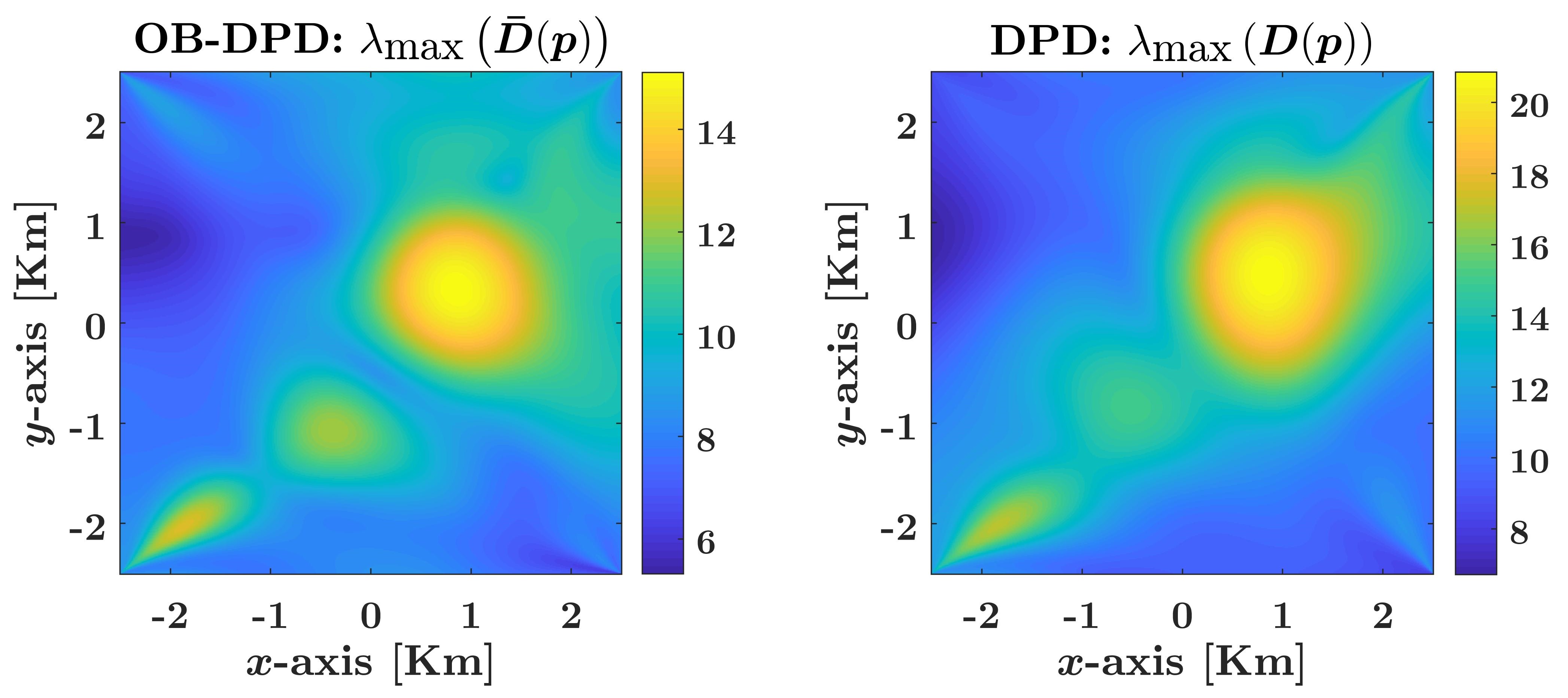
Fig. 1: Heat maps of OB-DPD and DPD, $\text{SNR}=0$[dB], $N=16$.

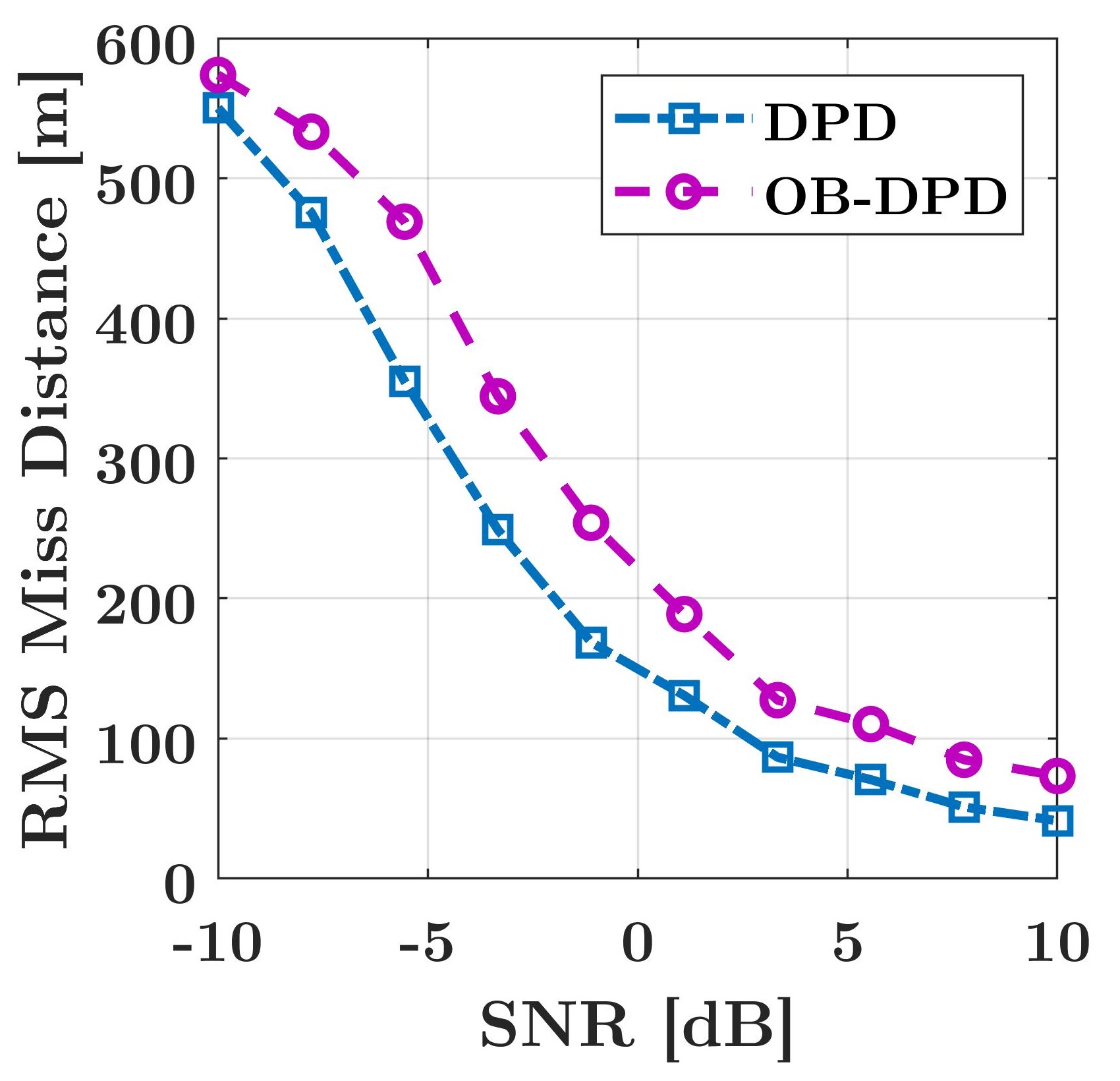
(a)

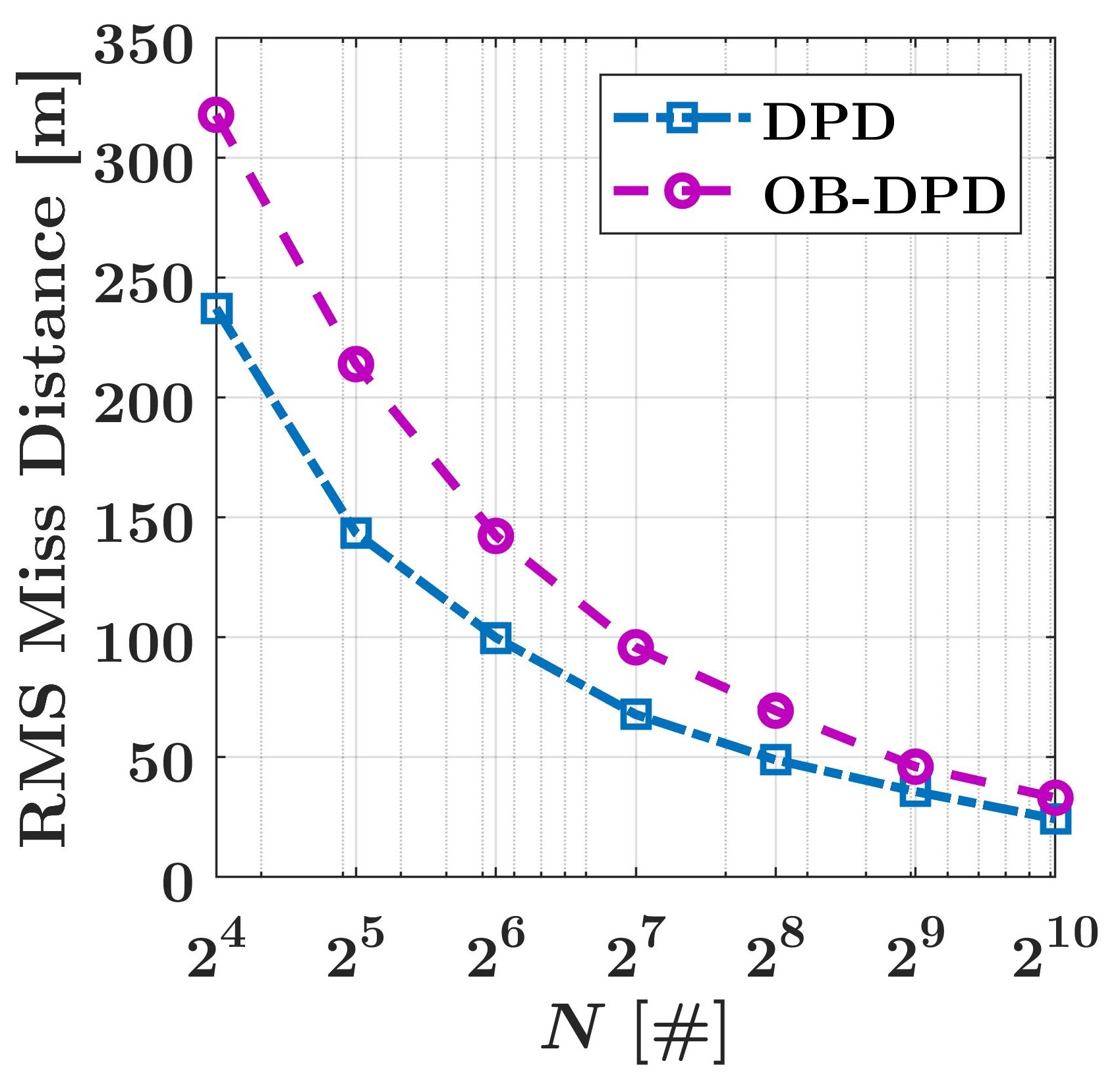
(b)

Fig. 2: RMS miss distance (a) vs. SNR, $N=32$ (b) vs. $N$, $\text{SNR}=0$[dB].

6 Conclusion

We presented a DPD method for one-bit quantized measurements of narrowband Gaussian signals. Based on the partial preservation of the SOS, we proposed the OB-DPD estimate, and established its asymptotic properties. We showed that the underlying signal model is subject to the same identifiability conditions of its respective “SOS-equivalent” quantization-free model. Relative to DPD without quantization, the requirements on the communication links between the base stations are significantly alleviated by OB-DPD, as the transmitted number of bits from each base station to the central processor is substantially reduced. Potential directions for future research are the quantification of information loss (in terms of estimation accuracy) due to the coarse one-bit quantization, extensions to multiple emitters, and to the more general case of non-Gaussian signals. Furthermore, an analytical analysis (approximately) predicting the minimal number of bits required from each station for a desired localization accuracy level, would be both instructive from a theoretical point of view, and beneficial from a practical point of view.

7 Acknowledgment

This work was supported, in part, by NSF under Grant No. CCF-1717610 and ONR under Grant No. N00014-19-1-2665.

References

• [1] Andrea Caiti, Andrea Garulli, Flavio Livide, and Domenico Prattichizzo, “Localization of autonomous underwater vehicles by floating acoustic buoys: a set-membership approach,” IEEE J. Ocean. Eng., vol. 30, no. 1, pp. 140–152, 2005.
• [2] Erik Ward and John Folkesson, “Vehicle localization with low cost radar sensors,” in IEEE Intelligent Vehicles Symposium (IV), 2016, pp. 864–870.
• [3] K. Becker, “Passive localization of frequency-agile radars from angle and frequency measurements,” IEEE Trans. Aerosp. Electron. Syst., vol. 35, no. 4, pp. 1129–1144, 1999.
• [4] Ryan W. Wolcott and Ryan M. Eustice, “Robust LIDAR localization using multiresolution gaussian mixture maps for autonomous driving,” Int. J. Robot. Res., vol. 36, no. 3, pp. 292–319, 2017.
• [5] Huaping Liu, Fuchun Sun, Bin Fang, and Xinyu Zhang, “Robotic room-level localization using multiple sets of sonar measurements,” IEEE Trans. Instrum. Meas., vol. 66, no. 1, pp. 2–13, 2016.
• [6] Liangtian Wan, Guangjie Han, Lei Shu, Naixing Feng, Chunsheng Zhu, and Jaime Lloret, “Distributed parameter estimation for mobile wireless sensor network based on cloud computing in battlefield surveillance system,” IEEE Access, vol. 3, pp. 1729–1739, 2015.
• [7] KC Ho and Wenwei Xu, “An accurate algebraic solution for moving source location using TDOA and FDOA measurements,” IEEE Trans. Signal Process., vol. 52, no. 9, pp. 2453–2463, 2004.
• [8] KC Ho, Xiaoning Lu, and La-or Kovavisaruch, “Source localization using TDOA and FDOA measurements in the presence of receiver location errors: Analysis and solution,” IEEE Trans. Signal Process., vol. 55, no. 2, pp. 684–696, 2007.
• [9] Anthony J Weiss, “Direct position determination of narrowband radio frequency transmitters,” IEEE Signal Proces. Lett., vol. 11, no. 5, pp. 513–516, 2004.
• [10] Anthony J. Weiss and Alon Amar, “Direct position determination of multiple radio signals,” EURASIP J. Appl. Signal Process., vol. 2005, no. 1, pp. 37–49, 2005.
• [11] Eric Miljko and Desimir Vucic, “Direct position estimation of UWB transmitters in multipath conditions,” in Proc. of IEEE ICUWB, 2008, vol. 1, pp. 241–244.
• [12] Marc Oispuu and Ulrich Nickel, “Direct detection and position determination of multiple sources with intermittent emission,” Signal Process., vol. 90, no. 12, pp. 3056–3064, 2010.
• [13] Tom Tirer and Anthony J. Weiss, “High resolution direct position determination of radio frequency sources,” IEEE Signal Process. Lett., vol. 23, no. 2, pp. 192–196, 2016.
• [14] Musa Furkan Keskin, Sinan Gezici, and Orhan Arikan, “Direct and two-step positioning in visible light systems,” IEEE Trans. Commun., vol. 66, no. 1, pp. 239–254, 2017.
• [15] Zhiyu Lu, Jianhui Wang, Bin Ba, and Daming Wang, “A novel direct position determination algorithm for orthogonal frequency division multiplexing signals based on the time and angle of arrival,” IEEE Access, vol. 5, pp. 25312–25321, 2017.
• [16] Yan-Kui Zhang, Hai-Yun Xu, Bin Ba, Da-Ming Wang, and Wei Geng, “Direct position determination of non-circular sources based on a doppler-extended aperture with a moving coprime array,” IEEE Access, vol. 6, pp. 61014–61021, 2018.
• [17] Fuhe Ma, Zhang-Meng Liu, and Fucheng Guo, “Distributed direct position determination,” IEEE Trans. Veh. Technol., 2020, doi: 10.1109/TVT.2020.3025386.
• [18] Junil Choi, Jianhua Mo, and Robert W. Heath, “Near maximum-likelihood detector and channel estimator for uplink multiuser massive MIMO systems with one-bit ADCs,” IEEE Trans. Commun., vol. 64, no. 5, pp. 2005–2018, 2016.
• [19] Yulong Gao, Deshun Hu, Yanping Chen, and Yongkui Ma, “Gridless 1-b DOA estimation exploiting SVM approach,” IEEE Commun. Lett., vol. 21, no. 10, pp. 2210–2213, 2017.
• [20] Jiaying Ren and Jian Li, “One-bit digital radar,” in Proc. 51st Asilomar Conference on Signals, Systems, and Computers, 2017, pp. 1142–1146.
• [21] Chun-Lin Liu and P.P. Vaidyanathan, “One-bit sparse array DOA estimation,” in Proc. of ICASSP, 2017, pp. 3126–3130.
• [22] Aria Ameri, Arindam Bose, Jian Li, and Mojtaba Soltanalian, “One-bit radar processing with time-varying sampling thresholds,” IEEE Trans. Signal Process., vol. 67, no. 20, pp. 5297–5308, 2019.
• [23] Xiaodong Huang and Bin Liao, “One-bit MUSIC,” IEEE Signal Process. Lett., vol. 26, no. 7, pp. 961–965, 2019.
• [24] Ziyang Cheng, Zishu He, and Bin Liao, “Target detection performance of collocated MIMO radar with one-bit ADCs,” IEEE Signal Process. Lett., vol. 26, no. 12, pp. 1832–1836, 2019.
• [25] Saeid Sedighi, Bhavani Shankar, Mojtaba Soltanalian, and Björn Ottersten, “One-bit DOA estimation via sparse linear arrays,” in Proc. of ICASSP, 2020, pp. 9135–9139.
• [26] Benedikt Loesch and Bin Yang, “Cramér-Rao bound for circular and noncircular complex independent component analysis,” IEEE Trans. Signal Process., vol. 61, no. 2, pp. 365–379, 2013.
• [27] Harry L. Van Trees, Optimum Array Processing: Part IV of Detection, Estimation, and Modulation Theory, New York: Wiley Interscience, 2002.
• [28] Michael J. Evans and Jeffrey S. Rosenthal, Probability and Statistics: The Science of Uncertainty, Macmillan, 2004.
• [29] Alan V. Oppenheim, John R. Buck, and Ronald W. Schafer, Discrete-Time Signal Processing, Upper Saddle River, NJ: Prentice Hall, 2001.
• [30] Robert M. De Jong, “Weak laws of large numbers for dependent random variables,” Annales d’économie et de statistique, pp. 209–225, 1998.
• [31] J. H. Van Vleck and David Middleton, “The Spectrum of Clipped Noise,” Proceedings of the IEEE, vol. 54, no. 1, pp. 2–19, 1966.
• [32] Giovanni Jacovitti and Alessandro Neri, “Estimation of the autocorrelation function of complex Gaussian stationary processes by amplitude clipped signals,” IEEE Trans. Information Theory, vol. 40, no. 1, pp. 239–245, 1994.
• [33] Henry B. Mann and Abraham Wald, “On stochastic limit and order relationships,” Ann. Math. Statist., vol. 14, no. 3, pp. 217–226, 1943.