SuperBoRG: Search for The Brightest of Reionizing Galaxies and Quasars in HST Parallel Imaging Data^†

Abstract

The Hubble Space Telescope (HST) has been providing tremendous survey efficiency via its pure-parallel mode, by observing another field in parallel with the primary instrument in operation for the primary observation. In this study, we present a new archival project, SuperBoRG, which aims at compiling data taken in extragalactic parallel programs of HST with Wide Field Camera 3 in the past decade; including pure-parallel (BoRG, HIPPIES, and COS-GTO) and coordinated-parallel (CLASH and RELICS) programs. The total effective area reaches $\sim$ $0.41\,\mathrm{deg}^{2}$ from $4.1$ Msec, or 47 days, of observing time, which is the largest collection of optical-to-near-infrared imaging data of HST for extragalactic science. We reduce all data in a consistent manner with an updated version of our data reduction pipeline, including a new sky background subtraction step. When available, imaging data from the Spitzer Space Telescope are also included in photometric analyses. The dataset consists of 316 independent sightlines and is highly effective for identification of high-$z$ luminous sources ($M_{\rm UV}\,\hbox to0.0pt{\lower 3.5pt\hbox{$\mathchar 0\relax\sim$}\hss}\raise 1.0pt\hbox{$<$}\,-20$ mag) at $z\sim 7$ to $12$, helping to minimize the effects of cosmic variance. As a demonstration, we present three new $z\,\hbox to0.0pt{\lower 3.5pt\hbox{$\mathchar 0\relax\sim$}\hss}\raise 1.0pt\hbox{$>$}\,7$ source candidates, including one luminous galaxy candidate at $z_{\rm phot}\sim 10.4$ with $M_{\rm UV}\sim-21.9$ mag; the best-fit spectral energy distribution implies a large amount of stellar mass ($\log M_{*}/M_{\odot}\sim 10$) and moderate dust attenuation ($A_{V}\sim 1.4$ mag), though the possibility of it being a low-$z$ interloper cannot completely be rejected ($\sim 23\%$) with the current dataset. The dataset presented in this study is also suited for intermediate and low-$z$ science cases.

[0.5em]0em1em

1 Introduction

The formation of the first stars, black holes, and galaxies is one of the central questions in current astronomical research. In particular, our understanding has been significantly advanced from the discovery of galaxies and quasars (e.g., Oesch et al., 2016; Bañados et al., 2018; Hashimoto et al., 2018; Yang et al., 2020) in the epoch of reionization (Gunn & Peterson, 1965; Madau et al., 1999; Becker et al., 2001; Robertson et al., 2015).

Significant contribution to our exploration into such an early epoch has been made by the Hubble Space Telescope (HST) since the installation of Wide Field Camera 3 (WFC3). The new camera has advanced our understanding of galaxies beyond the previous redshift limit, $z\sim 7$-8, and provided glimpses of galaxy formation in the early universe. A tremendous investment with the instrument has revealed hundreds of galaxy candidates at $z\,\hbox to0.0pt{\lower 3.5pt\hbox{$\mathchar 0\relax\sim$}\hss}\raise 1.0pt\hbox{$>$}\,7$ from various surveys; wide surveys like the Cosmic Assembly Near-infrared Deep Extragalactic Legacy Survey (CANDELS; Koekemoer et al., 2011; Grogin et al., 2011) and the Brightest of Reionizing Galaxies survey (BoRG; Trenti et al., 2011; Bradley et al., 2012), and deep surveys the Hubble Ultra Deep Field 2012 (HUDF12; Ellis et al., 2013), the Hubble eXtreme Deep Field (XDF Illingworth et al., 2013), Cluster Lensing And Supernova survey with Hubble (CLASH; Postman et al., 2012), the Hubble Frontier Fields (HFF; Lotz et al., 2017), and Reionization Lensing Cluster Survey (RELICS; Coe et al., 2019). Follow-up spectroscopic campaigns have successfully confirmed $\sim 20$ of those candidates at $z>7$ (e.g., Ono et al., 2012; Finkelstein et al., 2013; Oesch et al., 2015; Stark et al., 2015; Oesch et al., 2016; Song et al., 2016; Hoag et al., 2018; Hashimoto et al., 2018; Tamura et al., 2018). Some of them sources are surprisingly luminous (Zitrin et al., 2015; Oesch et al., 2016), exhibiting new interesting aspects of galaxy formation in the early universe, in conjunction with the formation of supermassive black holes as well (Mortlock et al., 2011; Bañados et al., 2018; Yang et al., 2020).

Bright sources are of particular interest from many perspectives; not only for their formation mechanisms in such an early epoch (e.g., Roberts-Borsani et al., 2020), but for their inferential application to cosmic reionization (Treu et al., 2013; Konno et al., 2014; Mason et al., 2018a; Hoag et al., 2019; Bañados et al., 2018; Davies et al., 2018). While low escape fraction of ${\rm Ly\alpha}$ photons is often the case for typical galaxies of luminosity $L<L^{*}$, situations seem dramatically different for luminous sources; theoretically, luminous sources are able to create a large ionizing bubble, where a higher fraction of ${\rm Ly\alpha}$ photons can escape (Cen & Haiman, 2000; Yajima et al., 2018; Mason & Gronke, 2020). Indeed, Stark et al. (2017) found a significantly high fraction of ${\rm Ly\alpha}$ detection in galaxies at $M_{\rm UV}<-20.3$ mag. A high escape fraction of luminous sources is also suggested from a double-peaked ${\rm Ly\alpha}$ line profile (e.g., Matthee et al., 2018). Therefore, luminous objects are ideal targets where we are likely to see ${\rm Ly\alpha}$ emission and gain insights into their properties (Mason et al., 2018b).

Such luminous sources are, on the other hand, rare ($\ll 10^{-5}$Mpc^-3; Bouwens et al., 2015), and thus significantly affected by cosmic variance (Trenti & Stiavelli, 2008; Robertson, 2010; Bhowmick et al., 2020). To obtain unbiased results from a single sightline, at least a $\sim 1$ deg² coverage will be needed at this redshift range (see Fig. 3 of Robertson, 2010), which is prohibitively expensive with WFC3 with its FoV of $\sim 4.7$ arcmin². A good example for such significant cosmic variance is that Roberts-Borsani et al. (2016) found three high-$z$ galaxies in one of the five CANDELS fields, EGS, whereas only one from the other four fields. Tilvi et al. (2020) recently revealed an over density of three galaxies at $z=7.7$, again in the EGS field. These examples clearly demonstrate that a survey of many sightlines, as a supplement to legacy-type surveys with a small number of sightlines, is necessary for unbiased measurements.

HST offers such an ideal opportunity via its pure-parallel observing mode—while the primary instrument is in operation, the secondary instrument can be used in parallel to observe a field a few arc-minutes away from the primary field. Since the coordinates of the pure-parallel field cannot be specified, pure-parallel opportunities are often used for identifying objects without any prior knowledge. That is, such opportunities are ideal to search for luminous rare objects in the early universe by minimizing the effects of cosmic variance (e.g., Atek et al., 2011). Previous pure-parallel observations in the BoRG program, which consist of $>1000$ HST orbits, have successfully identified $z>8$ galaxy candidates at the bright-end magnitude range, $M_{\rm UV}\sim-21$ to $-24$ mag (Schmidt et al., 2014b; Calvi et al., 2016; Bernard et al., 2016; Morishita et al., 2018). Identification of such luminous sources from sufficiently large volume is critical to determine the shape of the luminosity function and its evolution (Bowler et al., 2014, 2020; Bouwens et al., 2015; Ren et al., 2020).

The latest study of the BoRG collaboration has further extended their focus from galaxy candidates to unresolved point-source candidates in search of quasars and intense starburst galaxies at $z\,\hbox to0.0pt{\lower 3.5pt\hbox{$\mathchar 0\relax\sim$}\hss}\raise 1.0pt\hbox{$>$}\,8$ (Morishita et al., 2020). Identification of new quasars at high redshifts is of extreme importance—for example, theoretical studies expect that the evolution of the quasar luminosity function behaves differently depending on the mode of black hole evolution (Volonteri, 2010). In Morishita et al. (2020), they successfully identifies three point sources that satisfy color selection criteria for $z\sim 8$ objects. While spectroscopic confirmation is not yet available, the work demonstrated a new angle of using pure-parallel data of HST.

With its uniqueness and probing ability, pure-parallel fields with multi-band filters are of particular interest in the extragalactic community. Indeed, several follow-up studies have utilized data taken in previous BoRG campaigns and presented high-$z$ candidates independently selected by their criteria (e.g., Rojas-Ruiz et al., 2020), and some with addition of new data (Livermore et al., 2018; Bridge et al., 2019). However, due to a number of difficulties in selecting high-$z$ source candidates, different studies ended up having different sets of source candidates, despite using the same dataset. Such inconsistencies are often attributed to differences in error analyses, source detection and flux measurement, color selection criteria, and photometric redshift codes. Even a small discrepancy could eventually lead to conflicting conclusions on, e.g., the shape of the luminosity function at the bright-end magnitude range because not a large number of samples is currently available.

To alleviate possible systematics, in this study we initiate a new archival project, SuperBoRG. The primary purpose is to compile multi-band imaging data previously taken in parallel observations for extragalactic science cases, reduce them in a consistent manner, and publish data products for immediate use by the community. From both pure-parallel and coordinated-parallels programs with WFC3 in the past decade, we collect 316 sightlines with multi-band imaging data with moderate depth, which becomes one of the largest area extragalactic surveys conducted with HST. This unique dataset will be useful in many science cases; not only for high-$z$ source identification as previously presented by the BoRG collaboration, but for cosmology from clustering analysis (Robertson, 2010; Cameron et al., 2019), low- and intermediate-redshift galaxies, and even for foreground stars in our Galaxy (Ryan et al., 2011; Holwerda et al., 2014; van Vledder et al., 2016).

The contents of this paper are as follows: In Sec. 2, we present details on the data included in SuperBoRG, with a short description for each of parallel programs, as well as follow-up data by Spitzer. In Sec. 3, we describe details on reduction processes, including several changes to our customized reduction pipeline since Morishita et al. (2018), and present improvements by comparing with previous data products. In Sec. 4, we present photometric analysis, including photometry, redshift analysis, Spitzer photometry, which requires a separate reduction process due to its significantly large PSFs, and star-galaxy classification. In Sec. 5, as a demonstration of use of the data, we present new high-$z$ source candidates, and discuss possible caveats, while the entire list of high-$z$ candidates will be presented in a forthcoming paper. We describe the data products in Sec. 6, and summarize the paper in Sec. 7. Throughout, we quote magnitudes in the AB system.

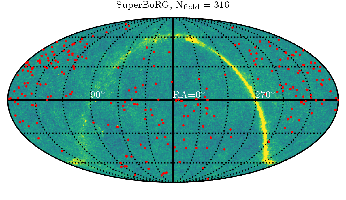
Figure 1: Distribution of SuperBoRG fields (red circles) in the ecliptic coordinates, overlaid on a temperature map from the WMAP 5-year data (Hinshaw et al., 2009). Most of the fields were selected from high Galactic latitudes ($|b|>30^{\circ}$), to avoid fields with significant Galactic extinction and/or dominated by foreground stars.

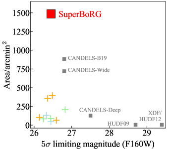
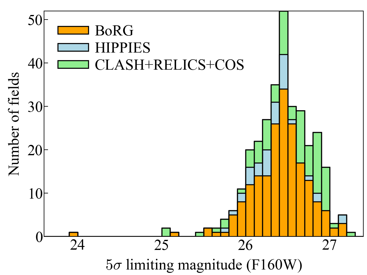
Figure 2: (Left): Effective area and $5\,\sigma$ limiting magnitude of various extragalactic survey programs of HST. Survey programs included in SuperBoRG (red square) are shown with cross symbols; BoRG cycles 17, 19, 22, 25 (orange), HIPPIES cycles 17, 18 (blue), CLASH, RELICS, and COS-GTO (green). Legacy surveys such as CANDELS, including its extended version presented in Bouwens et al. (2019, CANDELS-B19), and HUDF09/12/XDF programs are shown with gray squares. (Right): Histogram of limiting magnitude of the SuperBoRG fields (Sec. 3.1.3). Survey programs are distinguished by the same color scheme as in the left panel. The whole list for field coordinates and limiting magnitudes is summarized in Table 1.

2 Data: HST pure-parallel observations

In this SuperBoRG project, we collect fields from both pure-parallel and coordinated-parallel programs. The positional distribution in the sky is shown in Fig. 1, and area-magnitude distributions in Fig. 2. These selected fields have a sufficient number of broadband filters and depth for extragalactic science.

2.1 HST pure-parallel imaging data

2.1.1 BoRG

BoRG is a series of pure-parallel imaging programs initiated in 2009 (Trenti et al., 2011, 2012; Bradley et al., 2012). These programs were designed to search for luminous galaxies in the epoch of reionization, namely at $z\,\hbox to0.0pt{\lower 3.5pt\hbox{$\mathchar 0\relax\sim$}\hss}\raise 1.0pt\hbox{$>$}\,7$; thus observations were designed to efficiently identify high-$z$ objects via the Lyman break technique (Steidel et al., 1996), at a medium depth exposure with WFC3-UVIS and IR filters. Since its initiation, multiple programs have been awarded (Cycles 17, 19, 22, and 25; PIDs 11700, 12752, 13767, 15212), and the total number of HST orbits collected in the entire BoRG programs reaches $\sim 1400$.

Each of the BoRG programs has a different combination of filters, and thus selection criteria for high-$z$ galaxy candidates are different; however, there are basically three redshift ranges of interest, $z\sim 8$, 9, and 10, based on non-detection in WFC3-UVIS filters at $\,\hbox to0.0pt{\lower 3.5pt\hbox{$\mathchar 0\relax\sim$}\hss}\raise 1.0pt\hbox{$<$}\,1.0\,\mu{\rm m}$, and a color break measured with WFC3-IR filters. As an example, we present a few high-$z$ source candidates selected in this way in Sec. 5.2.

Filter sets of BoRG are also suited for identifying $z\sim 2$ galaxies, especially passively evolving galaxies with a strong Balmer break (e.g., Cameron et al., 2019). While the color break mimics the Lyman break at higher redshift, such degeneracy can be resolved by combining Spitzer data when available (Sec. 2.3).

The BoRG team has been adopting a carefully designed phase-II strategy since its initiation. For example, IR persistence in detectors is of particular concern because of the possibility of introducing an artificial coherent signal into the near-IR bands. Therefore, in each visit, they arranged the sequence of WFC3-IR filters to minimize the impact of persistence for the primary science goal, detection of dropout sources in blue filters such as F350LP and F105W. As detector persistence decays over time (with approximate power-law behavior), any saturated target observed in a previous visit most affects the initial part of the pure-parallel orbit. The general strategy therefore was to observe in these dropout filters as early as possible in each orbit (see Bradley et al., 2012, for more details).

It is noted that 7 fields of the Cycle 25 programs are discarded due to guide star acquisition failure during the entire visits. Many other fields were partially affected by similar failures. In fact, the fraction of guide star failures in the Cycle 25 fields is much higher than previous cycles, possibly due to the operational updates of HST, which originated from reduction of the number of gyros since 2018. Therefore, some of the Cycle 25 fields do not reach the depth that were originally designed.

Lastly, some of the BoRG fields had follow-up visits with WFC3 and ACS (PIDs 12905, 14652, 14701, 15702), primarily aiming at securing high-$z$ source candidates by adding medium-band imaging of WFC3-IR F098M (Livermore et al., 2018) and ACS F814W filter (Bridge et al., 2019). We include these data sets and reduce along with the primary data set.

2.1.2 HIPPIES

Hubble Infrared Pure Parallel Imaging Extragalactic Survey, HIPPIES, is also a series of pure-parallel imaging surveys carried out in Cycles 17 and 18 (PIDs 11702, 12286 Yan et al., 2011, 2012). While the filter sets of HIPPIES are similar to the one in the BoRG Cycle 17 campaign ($V$, $Y$, F125W, F160W), the program focused on fewer fields and spent longer exposure time in F098M (F105W) in Cycle 17 (Cycle 18), to secure $Y$-band dropouts. It is noted, due to a different phase-II design strategy, some of the data in Cycle 18 are significantly contaminated by IR persistence, and careful inspection is required when identifying dropout sources (See Sec. 5.2).

2.1.3 COS-GTO program

A part of the COS-GTO programs contains parallel imaging observations with WFC3 (PIDs 11519, 11520, 11524, 11528, 11530, 11533, 11534, 11541, 12036, 12024, 12025). The phase II of these programs was carefully designed for extragalactic science, in a similar way as in the BoRG programs (Trenti, M., private communication). The program provides 22 fields with multi-band images at medium depth. Some of the fields from this program also include additional UVIS filters that are not frequently used in other programs in SuperBoRG, such as F300X and F475X (with an extremely wide wavelength coverage), which improve sampling in spectral energy distribution (SED).

2.2 HST coordinated-parallel imaging data

Besides pure-parallel programs described above, we also include datasets from two coordinated-parallel programs spanning multiple fields: CLASH (Postman et al., 2012) and RELICS (Coe et al., 2019). While the primary targets of these programs are fields of massive clusters of galaxies at $z<1$, associated parallel fields are located $\sim 6$ arcmin away from the cluster center, and magnification effect is only a few percent if any.

2.2.1 CLASH program

Multi-band images from WFC3 were taken in 44 parallel fields during the primary imaging of 25 massive clusters of galaxies in the program Cluster Lensing And Supernova Survey With Hubble, CLASH (PID 12065; Postman et al., 2012). Most of the parallel fields consist of F350LP, F125W, and F160W filters, and primarily aimed at searching for high-$z$ SNe (e.g., Graur et al., 2014; Strolger et al., 2015; Riess et al., 2018). While the filter set technically allows $z\sim 10$ source selection (Sec 5.2), the fraction of low-$z$ interlopers is significantly high due to having a single non-detection filter and one color. All fields, however, have at least partial Spitzer IRAC ch1 and 2 coverage pointed at the cluster center (and ch3 and 4 for some fields), which improves the photometric redshift quality (Sec. 5.1).

Spectroscopic redshifts are also available for several fields, taken at VLT with VIMOS (Biviano et al., 2013; Balestra et al., 2016; Annunziatella et al., 2016; Monna et al., 2017), FORS2 (Biviano et al., 2013), and MUSE (Karman et al., 2015, 2017; Grillo et al., 2015; Caminha et al., 2016), as well as with HST grisms through the GLASS campaign (Schmidt et al., 2014a; Treu et al., 2015; Abramson et al., 2020). We retrieve publicly available redshift catalogs by the CLASH team, and cross-match with sources detected in this study. Since these spectroscopic campaigns were conducted primarily on the cluster center, the coverage in the parallel fields is partial; still, we find $90$ objects with a good spectroscopic quality (see Sec. 5.1).

It is noted that we exclude 6 fields of CLASH which are presented in the Hubble Frontier Fields (Coe et al., 2015; Lotz et al., 2017), as these imaging data are much deeper than the exposure time of typical fields in this study, and sophisticated catalogs are already available from several dedicated studies (Castellano et al., 2016; Shipley et al., 2018; Bradač et al., 2019).

2.2.2 RELICS program

Reionization Lensing Cluster Survey, RELICS (PID 14096; Coe et al., 2019; Salmon et al., 2020), is a HST Treasury Program, targeting 41 clusters at $0.18<z<0.97$ with the total of 188 orbits. Among 41 clusters, parallel fields were observed in 18 fields where no previous ACS imaging was available, spending $3$ orbits for each. The filters are set to those in the BoRG cycle 22 program, optimized for high-$z$ galaxy search, where F350LP is used for optical non-detection and four IR filters (F105W, F125W, F140W, and F160W) are used for dropout and color estimates. All parallel fields of RELICS have Spitzer IRAC ch1 and ch2 coverage, taken in part of the SRELICS program (Bradač et al., in preparation). Although images and photometric catalogs by the RELICS team are already available for these parallel fields, we start from the initial data reduction to have a consistent data set across the different survey programs presented in this study.

2.3 Spitzer IRAC data

While selection of high-$z$ source candidates requires multi-band images by HST, it is ideal to have additional photometric constraints at rest-frame optical wavelength range to effectively exclude low-$z$ interlopers with a similar SED (e.g., dusty star forming galaxies at $z\sim 2$; Sec. 5.1), as well as to better characterize their stellar properties. Mid-infrared coverage by Spitzer/IRAC plays such an important role by constraining SED at $>3\mu{\rm m}$ (e.g., McLure et al., 2011; Bradač et al., 2014; Bouwens et al., 2015).

There has been an effort by the BoRG team of following up fields with promising candidates, as well as by one of the most recent Spitzer DDT programs, COMPLETE2 (PID 14045; PI. Stefanon, M.). Typically, each of such fields has $\sim 1$ hr exposure with IRAC ch1 and ch2, which is sufficient for identification of low-$z$ interlopers down to $m_{160}\,\hbox to0.0pt{\lower 3.5pt\hbox{$\mathchar 0\relax\sim$}\hss}\raise 1.0pt\hbox{$<$}\,26$ mag, due to their red $m_{160}-[3.6]$ color. A few fields also have ch3 and ch4 coverage, taken for other targets nearby where these SuperBoRG fields are coincidently located within the FoV. For each field of SuperBoRG, we check availability of IRAC data, and reduce along with the primary HST dataset when available (Sec. 4.2).

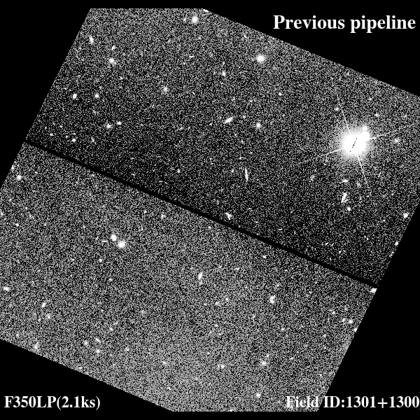
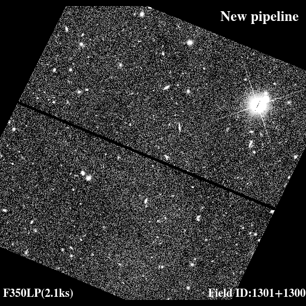
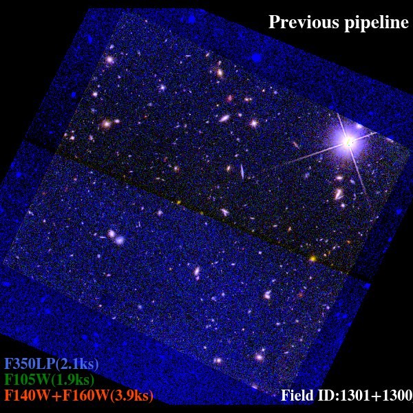
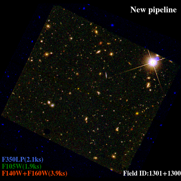
Figure 3: (Top) F350LP images of one of the SuperBoRG fields, sBoRG-1301+1300. The image from the previous pipeline (left) shows spatially varying sky residual in images and mismatched sky residual level between the two UVIS chips. The new pipeline resolves the issues (right), which also improves image photometric quality (see Fig. 4). (Bottom) Pseudo color images of the same field. Non-zero sky residual in F350LP filter is seen in the previous pipeline product, which is resolved in the new pipeline product.

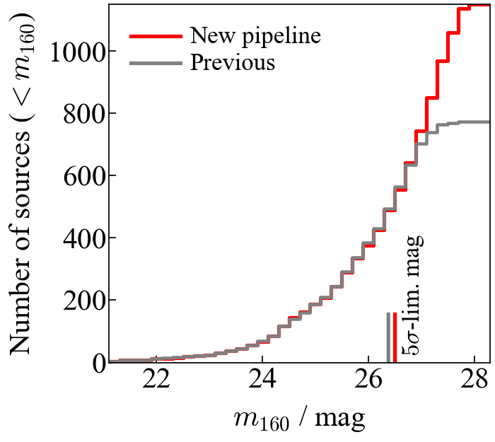
Figure 4: Cumulative distributions of sources detected in images from the previous pipeline (gray line) and the new pipeline (red) are shown. (The same field as in Fig. 3) The new pipeline product significantly improves detection at $\,\hbox to0.0pt{\lower 3.5pt\hbox{$\mathchar 0\relax\sim$}\hss}\raise 1.0pt\hbox{$>$}\,27$ mag, but also near the limiting magnitude, $\sim 26.5$ mag, which provides $\sim 0.1$ mag deeper limiting magnitude (vertical lines).

3 Reduction

3.1 HST image reduction

While pure-parallel opportunities provide us exceptional efficiency of mapping large areas of the sky, images taken in this mode are not dithered in most cases, as they cannot impact the primary observations, and thus careful post-processing is required. We use a dedicated pipeline, Borgpipe, originally designed for the BoRG data. A couple of updates are made in this study to improve the final data quality. The flow of the reduction process is as follows.

We start by visiting each field of the parallel programs above and retrieve all WFC3 and ACS images available via MAST. We download distortion-uncorrected imaging files: flt for WFC3IR, and flc for UVIS and ACS (i.e. Charge-Transfer Efficiency-corrected images; Noeske et al., 2012; Anderson, 2014). We check two header flags, QUALITY and EXPFLAG, of each retrieved image to identify any issues during the exposure, such as guide star acquisition failure and unexpected interruption, and discard those with problems.

We then check any satellite trails crossing images by using an automated algorithm provided in ACStools. The algorithm consists of three steps: 1. edge detection by using a Canny algorithm (Canny, 1986), to find boundaries in any given image by detecting discontinuities in the intensities from pixel to pixel which define the edge of a feature in the image, 2. clean step, by removing small objects whose perimeter is less than a certain number of connected pixels (75 by default), and 3. a Probabilistic Hough Transform (Galamhos et al., 1999), to look for straight line segments in the image (Borncamp & Lim, 2016, for more details). We use a set of parameters suggested by the ACS team, which was found sufficiently effective in our initial test using a subset of data with satellite trails. Detected satellite trails in each flt/flc file are masked by changing the value in the DQ array so the contaminated pixels are not used in the following reduction.

We then perform a customized cosmic ray (CR) rejection, by using the python version of the Laplacian edge filtering algorithm (LACOSMIC; van Dokkum et al., 2001). We set cr_threshold to $2.3\,\sigma$ and $3.0\,\sigma$ for UVIS and IR detectors, respectively, from our dedicated test in Morishita et al. (2018). It is noted that an aggressive setup detection for the CR detection in the optical band may cause false identification of dropout sources by removing positive pixels in bluer bands as CRs.

These cleaned images are then aligned within each filter by using Tweakreg and then combined. The combined images are then aligned to the F160W image before the final drizzle step. We also attempt to align the combined images to GAIA DR2 astrometry frame (Gaia Collaboration et al., 2018) when more than three stars are available. While image distortion and misalignment are automatically corrected by Tweakreg, we carefully inspect the final data product, and tune configuration parameters field-by-field when necessary.

While astrodrizzle performs sky background subtraction during the final drizzle step, it only subtracts a global sky value estimated from the entire detector. We found that some images show noticeable amounts of sky flux spatially varying across the detector (Fig. 3). Also, the two UVIS chips often show mismatched residual flux levels, which implies a more sophisticated method of sky background subtraction is required. To overcome this issue, we develop an alternative approach for sky subtraction by using SExtractor. For each flt/flc image we run SExtractor and subtract the output background image from the original image. Parameters of SExtractor for source detection and background size at this stage are very critical to final output products. We carefully accessed results in a subset of data, and optimized these parameters to BACK_FILTERSIZE 6 (10) and BACK_SIZE 250 (500) for WFC3-IR (WFC3-UVIS and ACS) data. The comparison between the original sky-subtraction method is shown in Sec. 3.1.1.

Lastly, sky-subtracted images are combined with a common pixel scale of $0.\!\arcsec 08$ / pixel and with pixfrac to 0.75, optimized for our non-dithered images from previous studies. The sky subtraction step here is skipped to avoid duplication. This final step produces science and rms maps for each filter band, as well as a combined F140W+F160W image for source detection and optical-stacked image (combined with filters bluer than F098M) for optical non-detection of high-$z$ candidates.

3.1.1 Background subtraction

In Fig. 3, we show one example field of SuperBoRG that shows significant background residual in F350LP. The final image processed with the previous pipeline shows spatially varying background residual across each of the two UVIS detector chips. In addition, the residual levels of the two chips are not matched. These residual features are clearly noticeable in a pseudo rgb color image shown in Fig. 3. The final images processed with our custom sky subtraction step are shown in the right panels, where we can see uniform flux distribution across the detector.

Figure 4 shows magnitude distributions of sources detected in F160W images from the previous and new pipelines. While the number of detected sources in the new pipeline image remains similar at $\,\hbox to0.0pt{\lower 3.5pt\hbox{$\mathchar 0\relax\sim$}\hss}\raise 1.0pt\hbox{$<$}\,26$ mag, significant increase is seen at fainter magnitude, by detecting additional $\,\hbox to0.0pt{\lower 3.5pt\hbox{$\mathchar 0\relax\sim$}\hss}\raise 1.0pt\hbox{$>$}\,400$ sources in total. While these additional sources are fainter than the flux limit for science use in most cases, it is still important to locate these sources and, for example, mask when necessary to avoid any flux blending to a source of interest. An error analysis of the images (see Sec. 3.1.3 for details) indeed reveals $\sim 0.1$ mag improvement in its limiting magnitude.

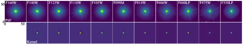
Figure 5: (Top) Median-combined PSFs of primary filters. Individual PSFs are collected from SuperBoRG fields and then cross-matched with the GAIA DR2 catalog to ensure the selection of stars. (Bottom) Convolution kernels for each PSF used for PSF-matching to the F160W PSF, generated by pypher.

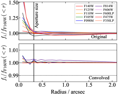
Figure 6: (Top) Total flux of original PSFs normalized by flux of the F160W PSF within a radius. (Bottom) Same as top panel, but after convolving PSFs with kernels generated by pypher. The difference remains $<0.3\%$ for all filters at a radius of aperture photometry, $r=0.\!\arcsec 32$.

3.1.2 PSF matching of images

In the previous works of BoRG, images were not matched to a common point-spread function (PSF) size, partially due to lack of accurate PSF characterization. Instead, flux measurement has been conducted by the ISOPHOTAL mode of SExtractor, which collects flux in a segment defined in the detection image. However, flux estimated in ISOPHOTAL can be significantly underestimated in blue filters, which may cause an artificial dropout, especially when images are not dithered (Sec. 4.1.1). Since we collect a sufficiently large number of fields through a consistent reduction process, we here endeavor to improve photometric quality by matching image PSFs and adopting a canonical aperture photometry.

To have image PSFs matched between different filters, we first collect PSFs from the entire SuperBoRG fields. We identify bright, but not saturated stars ($16.5<m/{\rm mag}<22$) from reduced images. To make sure only stars are collected, we cross-match identified objects with the GAIA DR2 catalog (Gaia Collaboration et al., 2018). For each of those selected stars, we cut out into a postage stamp, subtract its local sky, and normalize the total flux. Due to a relatively large pixel size of SuperBoRG, we resample each star into a $10\times$ smaller pixel scale size and shift the image to its light-weighted center before the final median-stack in each filter. The median-stacked PSFs of our primary filters are shown in Fig. 5. These PSFs are then provided to Pypher (Boucaud et al., 2016), to generate matching kernels to the F160W PSF (also shown in Fig. 5). We investigate encircled fluxes of convolved PSFs in Figure 6. The radial light profiles of convolved PSFs show a difference of $<0.1\%$ from the F160W PSF at radius $r=0.\!\arcsec 32$ i.e. aperture size for our photometry (Sec. 4.1).

Due to a small number of available images, some filters do not have sufficient stars for characterizing its PSF. We therefore approximate these PSFs by using one close to these filters (F350LP for F300X and F435W, F606W for F555W and F625W, and F814W for F775W and F850LP). An alternative solution for this would be Tiny Tim PSFs (Krist, 1995). However, it is known that Tiny Tim PSFs show non-negligible offsets at the inner part of a light profile (van der Wel et al., 2012; Bruce et al., 2012; Morishita et al., 2014). To avoid such additional uncertainty, we proceed with the empirical approximation for these filters. It is noted that these filters appear only in a couple of fields. Furthermore, these filters are primarily used for non-detection in the selection of high-$z$ source candidates, and thus our approximations of these PSFs do not significantly affect the final result.

3.1.3 Error analysis

It is known that photometric flux error of HST images measured by SExtractor is underestimated, primarily due to correlation between pixels (Casertano et al., 2000). Root mean square (RMS) maps generated by our pipeline thus need to be scaled so that it represents more realistic uncertainty.

To estimate the scaling factor, we follow the method presented in Trenti et al. (2011). Briefly, we place 100 apertures in randomly selected empty (i.e. devoid of real sources) regions of each image, and measure fluxes therein by using SExtractor (Bertin & Arnouts, 1996). The configuration parameters and aperture diameter size are set identical to those used for detection of real sources ($0.\!\arcsec 64$; Sec. 4.1). Each RMS map is then scaled so that the standard deviation of fluxes of the empty apertures ($\langle f_{aper}\rangle$) and the median of flux errors returned by SExtractor ($\langle e_{aper}\rangle$) are matched. We repeat this analysis for 10 times, with a new set of random apertures, and take the median of scaling factors calculated at each realization. Scaling factors here are generally larger than previous studies (e.g., Morishita et al., 2018). We attribute this to the PSF matching process in this study, which increases correlation between pixels. The distribution of $e_{aper}$ is also used to estimate limiting magnitudes for the following analysis. A histogram of F160W limiting magnitudes ($5\,\sigma$) of the entire SuperBoRG fields is shown in Fig. 1, characterizing $\sim 26.5$ mag as the median limiting magnitude.

3.2 Spitzer image reduction

We check IRAC image availability for every SuperBoRG field at the Spitzer heritage archive, and retrieve imaging data of IRAC channels 1 and 2, in the level1 format (pbc) when available. We use the Spitzer Science Center reduction software MOPEX (Makovoz & Marleau, 2005) to reduce images. After background subtraction and alignment of each pbc image, we combine images by setting the final pixel scale to $0.\!\arcsec 54$ and pixel fraction to 0.4. Combined images are then aligned to the detection image of HST in the field.

The combined images are then resampled to the same pixel size of HST, $0.\!\arcsec 08$, as a matched pixel scale is required by the flux extraction code for these images (Sec. 4.2). We use an astropy module, reproject for image resampling. As for HST images, Spitzer images need correction for the correlated noise. RMS scaling factors and limiting magnitudes are estimated in the same manner as for HST images, by measuring RMS in empty regions, but using a larger aperture of diameter size $0.\!\arcsec 54$ (Sec 3.1.3). Among the SuperBoRG fields, 156 (121) fields have IRAC ch1 (ch2) coverage. Limiting magnitudes of IRAC images are summarized in Table 1.

4 Photometric properties

4.1 HST Photometry

For each field, sources are detected with SExtractor in the F140W+F160W detection image. Detection parameters are set as follows—DETECT_MINAREA $=9$, NTHRESH $=0.7\,\sigma$, DEBLEND_NTHRESH $=32$, DEBLEND_MINCONT $=0.001$. A relatively large convolution size ($5$ pixels for FWHM of Gaussian) for detection is used to reduce false detection of, e.g., discrete noise at the edge of the detector and residual cosmic rays. Photometry for each filter is conducted in the dual-imaging mode based on the detection image. Signal-to-noise ratios are calculated from flux and error measured in an aperture with diameter size of $0.\!\arcsec 64$. We scale measured flux to the total flux, by multiplying the ratio of total flux ($f_{\rm auto,F160W}$) and aperture flux ($f_{\rm aper,F160W}$) measured in F160W band uniformly to all filters.

Once fluxes are measured and scaled, Galactic dust reddening is corrected by using the attenuation value retrieved for each coordinate from NED (Schlegel et al., 1998; Schlafly & Finkbeiner, 2011). We adopt the canonical Milky Way dust law (Cardelli et al., 1989).

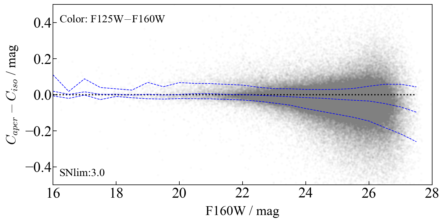
Figure 7: Comparison of aperture and isophotal photometry for sources with $S/N_{\rm F160W}>3$ and $\rm f_{persist}=0$. Colors, here F125W$-$F160W, are broadly consistent down to $\sim 24$ mag. At fainter magnitudes, however, the color measured by the isophotal photometry ($C_{\rm iso}$) systematically becomes redder than the one by the aperture photometry ($C_{\rm aper}$), which could result in false identification of high-$z$ dropout sources (Sec. 4.1.1). Running 16/50/84th percentiles (blue dashed lines) and the zero point (black dotted line) are shown.

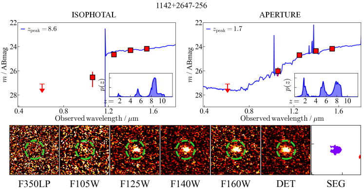
Figure 8: Example of misidentification of a low-$z$ source as a high-$z$ source candidate by adopting isophotal flux. This object, sBoRG-1142+2647-256, was originally identified as a z8_Y105 candidate, by its strong dropout in F105W isophotal flux, with a primary peak at $z=8.6$ (left). The object, however, is excluded from the selection when aperture flux is used; F105W flux becomes more significant, and it is more likely a low-$z$ interloper, with a primary peak at $z=1.7$ (right). Such misidentification can happen because the isophotal measurement collects flux from pixels defined in the segmentation map (“SEG”) uniformly for all filters, where more noise would be involved in bluer filers and lead to underestimation of S/Ns. On the other hand, aperture photometry collects flux from a defined aperture ($r=0.\!\arcsec 32$; half the size of green circles), which is typically smaller than the area defined in the segmentation map, and provides more reliable flux measurements.

4.1.1 Comparison between aperture and isophotal fluxes

In previous studies of BoRG, the isophotal photometry (FLUX_ISO of SExtractor) has been a standard way of flux measuring. The isophotal photometry is known to accurately measure colors based on the detection map inferred from the detection image when the dual-imaging mode of SExtractor is used. In addition, it does not necessarily require images to be PSF-matched beforehand, whereas this is not the case for aperture photometry, where having a consistent central light profile is critical for unbiased measurements. While the isophotal photometry has often been proved effective when images are dithered, this is not always true for non-dithered images, as having a large detection area may introduce contamination by unmasked bad pixels and CRs.

To investigate this, we first compare colors (here F125W$-$F160W) derived with isophotal and aperture photometry in Fig. 7. As is expected, these colors are broadly consistent down to $\sim 24$ mag. However, at a fainter magnitude range, which is typical for high-$z$ sources, the color derived by isophotal photometry is systematically redder than the aperture color, implying that the former could identify more high-$z$ source candidates.

In Fig. 8, we showcase an example of false identification of a high-$z$ source candidate by this effect. The object was originally identified as a $z\sim 8$ candidate, from its striking break color in F105W$-$F125W measured with the isophotal photometry. Indeed, photometric redshift analysis shows a primary peak at $z=8.6$. The object, however, is not selected as a high-$z$ candidate when the aperture photometry is used instead, as the estimated flux of F105W becomes more significant (i.e bluer break color), and it is found more likely to be a low-$z$ interloper at $z\sim 2$.

Such misidentification of high-$z$ sources (see also Appendix of Morishita et al., 2018) probably occurs because isophotal flux collects flux from pixels defined in a segmentation map (“SEG” in Fig. 8), uniformly in all filters. Segmentation maps are often defined in red filters (here F140W+F160W image), and the region defined in such a way is larger than the actual size of the object in blue filters for many extragalactic sources. This would then include more empty pixels (i.e. noise) in flux measurement in bluer filers, and lead to underestimation of S/N. On the other hand, aperture photometry collects flux in an aperture defined, and by having a reasonably small aperture, such bias can be mitigated, though it requires images having matched PSFs. Given that our PSF-matching quality turns out to have $\ll 1\%$ accuracy from the previous section, we choose aperture photometry for the following photometric analysis.

4.2 Spitzer Photometry

Since IRAC images have much larger PSFs ($0.\!\arcsec 18$), deblending source flux from surrounding sources is a critical step for accurate characterization. To extract source flux in IRAC images, we use the T-PHOT package (Merlin et al., 2016). TPHOT estimates flux in a low-resolution (LR) image based on structure in a high-resolution (HR) image. We use the $JH_{\rm 140}$+$H_{\rm 160}$ detection image as the HR image for each field, and convolution kernels required by TPHOT are generated by stacking PSFs found in IRAC images. We resample Spitzer images in the same scale as for the HR image and provide those to TPHOT.

We extract sources down to $m_{160}=24$ mag uniformly for all fields where IRAC images are available. Those with extracted flux fainter than the limiting magnitude of each IRAC image, however, are replaced with the limiting magnitude as upper limit. TPHOT also returns a flag for extraction, to inform the user if the target object is blended with neighboring ones. We include the flag for all IRAC channels in the final photometric catalog.

For sources fainter than $m_{160}=24$ mag, we do not perform the flux extraction process by TPHOT, as including such faint sources could occasionally cause a crash during the fitting stage. However, high-$z$ source candidates identified in SuperBoRG (Sec. 5.2) are often fainter than this magnitude, and an extra flux extraction process is required. For those selected as high-$z$ source candidates, we follow a method presented by Morishita et al. (2020), which models the LR light profile using GALFIT based on the profile parameters derived from HR images. Since this method concerns a smaller cutout and is computationally intensive, we only use this extraction method for sources of particular interest (Sec. 5.3).

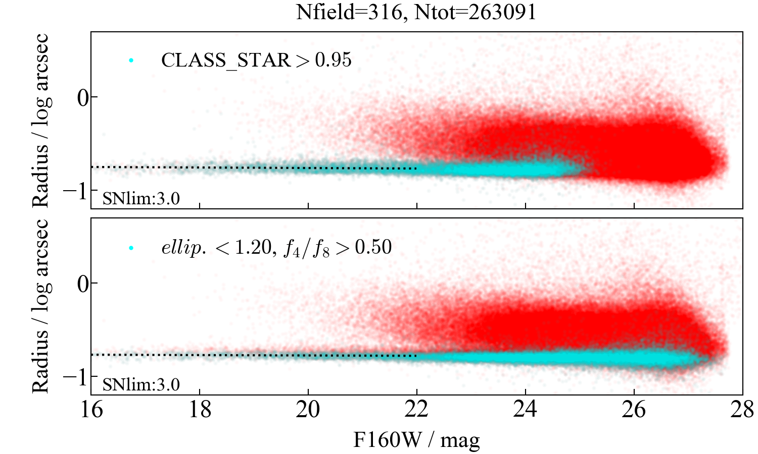
Figure 9: Distribution of sources with $S/N_{\rm F160W}>3$ and $\rm f_{persist}=0$ (red dots), in a size-magnitude plot. Those selected as point sources using CLASS_STAR (top) and a combination of ellipticity and flux concentration (bottom) are highlighted (cyan dots). Slopes fit to the selected point sources are also shown (black dashed lines).

4.3 Point-source selection

In Fig. 9, we show the size distribution of all sources with $S/N>3$, where the size is a non-parametric half-light radius (FLUX_RADIUS) derived with SExtractor. Traditionally, CLASS_STAR (a float number that ranges from 0 to 1, where a source is more likely a point source as the number increases) has been used as a useful parameter for star-galaxy classification. Those with CLASS_STAR $>0.95$ tightly distribute at the lower edge of the distribution up to $\sim 24$ mag. However, as previously indicated (Finkelstein et al., 2015; Morishita et al., 2020), the flag is not complete at fainter magnitudes.

Instead, Morishita et al. (2020) demonstrate an alternative classification for point sources using ellipticity ($e$) and flux concentration, specifically,

$$e<1.2\wedge f_{4}/f_{8}>0.5$$ (1)

where $f_{x}$ is flux measured within an aperture of $r=x$ pixels. Sources selected with the criteria are shown in the bottom panel of Fig. 9, where we see a tight distribution extending down to a fainter magnitude, $\sim 26$ mag, providing a good alternative way of separating point and extended sources. With this optimization down to fainter magnitudes, this criterion, in combination with color criteria presented below, can also be applied for high-$z$ point-source selection, in search of quasars and starburst galaxies (see Section 5.2, and Morishita et al., 2020, for comprehensive analyses and discussion).

It is noted that there is a fraction of sources with CLASS_STAR $>0.95$ that do not satisfy the criteria at the bright-end magnitude range, $<22$ mag. Most of such sources are on the upper side of the sequence, which implies that the method offers a more conservative, but possibly incomplete way of separating point sources. It is noted that sources selected in both selection criteria show a flat slope of similar intercepts ($\log r/{\rm arcsec}=-0.76$ and $-0.78$, respectively). Sources with measured size below this limit should be considered as unresolved.

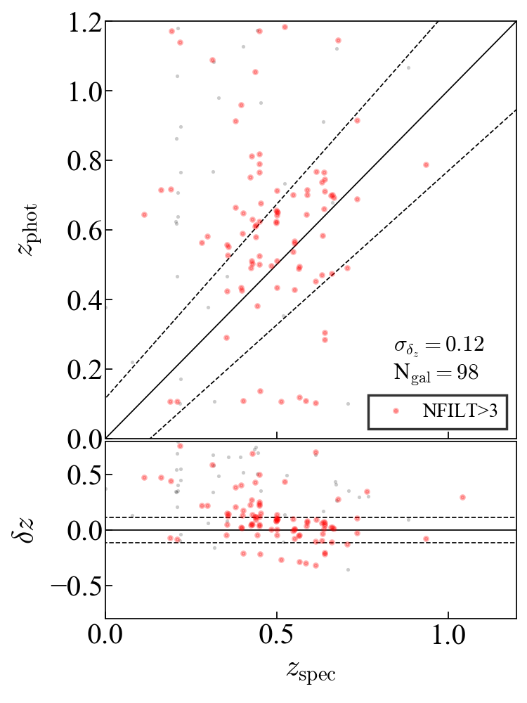
Figure 10: Comparison of photometric and spectroscopic redshifts of objects taken from the CLASH fields. For photometric redshift, we use zmc, which is calculated based on the posterior distribution, instead of zpeak, to overcome relatively few numbers of filters in these fields. Scatter is defined by $\delta z=(z_{\rm phot}-z_{\rm spec})/(1+z_{\rm spec})$. Objects with more than 3 filters (red circles; $N=98$) are used for calculating the median of scatter, $\sigma_{\delta_{z}}\sim 0.12$ (dashed lines), while the rest are also shown ($N=94$; gray dots).

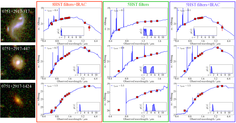
Figure 11: Example of three low-$z$ galaxies from the sBoRG-0751+2917 field, where a sufficient number of filters are available for a phot-$z$ comparison test. Each row shows results of individual galaxies, with a full set of filters (left), 5 HST filters as a fiducial example for BoRG (middle), and 5 HST filters and 2 Spitzer filters (right). Redshift probability distributions are shown in the inset. Multiple redshift peaks seen in the results with the HST-only filter set are resolved by adding Spitzer filters.

5 Analyses

5.1 Photometric Redshift

We derive photometric redshifts by using EAzY (Brammer et al., 2008), with its default template set (v1.3) and configuration parameters. The fitting redshift range is set to $z\in[0.01,12]$ with a step size of $\Delta\log(z+1)=0.01$. We use the default prior provided by EAzY, where brighter sources in F160W are more likely to be at lower redshift (see also Morishita et al., 2017). Those who wish different configuration setups can use the flux catalog we provide and repeat the analysis.

We calculate absolute UV magnitude ($M_{\rm UV}$) and rest-frame colors by using the best fit SED at $z_{\rm peak}$. $M_{\rm UV}$ is calculated at rest-frame 1450 Å. Rest-frame colors, $U-V,B-V,V-J,z-J$, are calculated by convolving the best fit SED with filter response curves of standard filters.

While most of the SuperBoRG fields are not covered spectroscopically, an exception is the CLASH program. Several fields of CLASH have spectroscopic follow-up observations, through the VLT-CLASH campaign (Sec. 2.2.2). In Fig. 10, we compare our photometric redshifts to spectroscopic ones taken from the catalogs published by the CLASH team. Since most of the spectroscopic sources are relatively bright galaxies at $z<1$, we here use zmc for photometric redshift, which is calculated from the posterior probability distribution with the F160W magnitude prior. The scatter is measured by $\delta z=(z_{\rm phot}-z_{\rm spec})/(1+z_{\rm spec})$, where we have $\langle\delta z\rangle=0.12$ for 98 objects with reliable spectroscopic redshift ($>80\%$) and a sufficient number of filters ($>3$) for photometric redshift calculation. Adopting $z_{\rm peak}$ instead of zmc returns a larger scatter and higher fraction of catastrophic outliers, as the data set cannot distinguish, e.g., $z\sim 1$ and $z\sim 4$ solutions without the prior information in many cases (see below).

Since most of the CLASH fields typically have fewer filters than other programs, we also show an example of photometric redshift analysis on galaxies taken from the sBoRG-0751+2917 field, where 8 HST+IRAC filters are available (Fig. 11). The field was originally observed in the cycle 17 HIPPIES program, and then followed up by Spitzer with IRAC ch1 and 2. We select three low-$z$ galaxies with different features; blue spiral galaxy, green disk+bulge galaxy, and passively evolving galaxy. With the full filter set, photometric redshift is well constrained, with a single peak in its probability distribution in all three cases. It is also noticed that Spitzer photometry plays an important role by constraining rest-frame $1.5\mu{\rm m}$ i.e. dust reddening and emission from low-mass stars; as a result, the derived redshift distribution has a single peak in all cases.

To test photometric redshift quality of the same objects with reduced numbers of filters, we simply repeat the redshift fitting process for the same galaxies with the following two setups; 1. one with only 5 HST filters (F350LP, F105W, F125W, F140W, and F160W), a default filter set for many of the SuperBoRG fields, and 2. the same 5 HST filters plus 2 IRAC filters. The results are shown in Fig. 11.

With only HST filters, the probability distribution shows multiple peaks, which can be attributed to the fact that the set of filters only covers rest-frame $\sim 0.4$ to $1\mu{\rm m}$ wavelength range and cannot distinguish degeneracy between the Balmer break at $z\sim 1$ and the Lyman break $z\sim 4$. Fields with a few number of HST filters therefore may need additional setups e.g., by including redshift priors based on source morphology (Coe et al., 2006), luminosity (Brammer et al., 2008) and/or environment (Morishita et al., 2017), when used for low-$z$ science cases. Adding IRAC photometry, on the other hand, returns a singly peaked redshift distribution, by constraining rest-frame $\sim 2\mu{\rm m}$ wavelength range. The distribution is already similar to, but slightly broader than, the one derived with the full filter set.

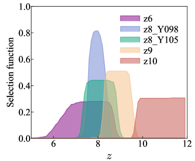
Figure 12: Effective redshift windows of the photometric color selections presented in Sec. 5.2. Distributions are normalized to an arbitrary constant.

5.2 Color selections for high-z candidates

To select high-$z$ source candidates, we follow color selection criteria defined in previous studies of the BoRG collaboration (Schmidt et al., 2014b; Calvi et al., 2016). The color selection method is based on the Lyman break technique (Steidel et al., 1996), with some additional color cuts to effectively exclude low-$z$ interlopers. Signal-to-noise ratios and colors used in the following criteria are calculated with the aperture flux of $0.\!\arcsec 64$ diameter.

In addition to color-cut criteria presented in the following subsections, we apply the following photometric cut uniformly to all high-$z$ source candidates;

$$S/N_{\rm non-detection\ filters}<1.0$$

$$S/N_{\rm min.,non-detection\ filters}<1.0$$

$${\rm f_{persistent}=0}$$

Non-detection filters are defined in each redshift range below, and objects without any non-detection filter coverage are excluded from the candidate list. In addition to the non-detection measured in a $0.\!\arcsec 64$ diameter aperture ($S/N_{\rm non-detection\ filters}$), we measure $S/N$ in the non-detection filters with a smaller aperture ($0.\!\arcsec 16$ diameter) to secure non-detection ($S/N_{\rm min.,non-detection\ filters}$). For the same reason described in Sec.4.1.1, having unnecessarily large apertures can underestimate S/N and falsely identify an object as non-detection.

${\rm f_{persistent}}$ is a flag for IR persistence. Specifically, for each of selected candidates, we visit IR persistent model images created for each visit of the field, and check if the source position is affected by persistence. If there is any overlap between the segmentation map of the source and the flagged area in the IR persistence model, the object is flagged (${\rm f_{persistent}}=1$) and excluded from the candidate list.

5.2.1 $z\sim 10$ galaxy candidates

$$S/N_{\rm 160}>6.0$$

$$J_{125}-H_{160}>1.3$$

$$H_{160}-[3.6]<1.4\ {\rm(when\ IRAC\ ch1\ is\ available)}$$

(z10 selection). Non-detection filters are F105W and bluer filters. The additional $H_{160}-[3.6]<1.4$ cut, only when IRAC ch1 is available, offers more robust candidates (Bouwens et al., 2015).

5.2.2 $z\sim 9$ galaxy candidates

$$S/N_{\rm 140}>6.0\land$$

$$S/N_{\rm 160}>4.0\land$$

$$Y_{105}-JH_{140}>1.5\land$$

$$JH_{140}-H_{160}<0.3\land$$

$$Y_{105}-JH_{140}>5.33\cdot(JH_{140}-H_{160})+0.7$$

(z9 selection). Non-detection filters are F098M and bluer filters.

5.2.3 $z\sim 8$ galaxy candidates

For fields where F105W filter is available,

$$S/N_{\rm 125}>6.0\land$$

$$S/N_{\rm 160}>4.0\land$$

$$Y_{105}-J_{125}>0.45\land$$

$$J_{125}-H_{160}<0.5\land$$

$$Y_{105}-J_{125}>1.5\cdot(J_{125}-H_{160})+0.45$$

(z8_Y105 selection). Non-detection filters are F814W and bluer filters.

For fields where F098M filter is available,

$$S/N_{\rm 125}>6.0\land$$

$$S/N_{\rm 160}>4.0\land$$

$$Y_{098}-J_{125}>1.75\land$$

$$J_{125}-H_{160}<0.5\land$$

$$(J_{125}-H_{160})<0.02+0.15(Y_{098}-J_{125}-1.75)$$

(z8_Y098 selection). Non-detection filters are F814W and bluer filters.

5.2.4 $z\sim 6$ galaxy candidates

For fields where F814W filter is available,

$$S/N_{\rm 125}>6.0\land$$

$$S/N_{\rm 160}>4.0\land$$

$$I_{814}-J_{125}>0.8\land$$

$$J_{125}-H_{160}<0.4\land$$

$$I_{814}-J_{125}>2.0\cdot(J_{125}-H_{160})+0.8\land$$

(z6 selection). Non-detection filters are F606W and bluer filters. It is noted that, as shown in Fig. 12, this selection has a wide selection window in the redshift space, partially overlapping with other selections at $z\sim 7$ to 8. However, having this selection is still effective in a field where no $Y$-band is available, which is occasionally the case for some of the BoRG cycle 25 and CLASH fields. We still keep the same labeling, “z6”, as in the original reference of this selection (Bouwens et al., 2015), whereas the median of the probability distribution is $z\sim 7.5$.

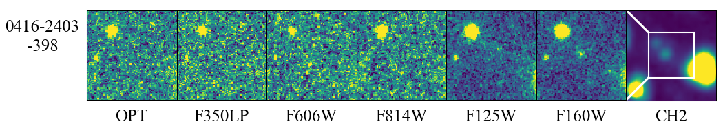
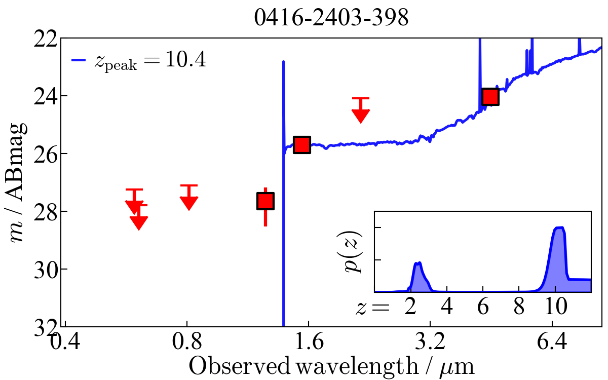
Figure 13: High-redshift source candidate sBoRG-0416-2403-398 identified in the z10 selection. The redshift probability distribution peaks at $z\sim 10.4$ with $M_{UV}=-21.9$ mag, characterizing this as one of the most luminous candidates at $z\sim 10$ in the literature. Significant detection in IRAC ch2, however, implies that the object could be a $z\sim 3$ dusty galaxy instead, with $p(z<6)=23\%$. Postage stamps are $6.\!\arcsec 5\times 6.\!\arcsec 5$ in size for HST and $12.\!\arcsec 8\times 12.\!\arcsec 8$ for Spitzer ch2. The size of the HST stamps is shown in the Spitzer image (white rectangle). OPT is for a stacked image of optical bands (F814W and bluer filters).

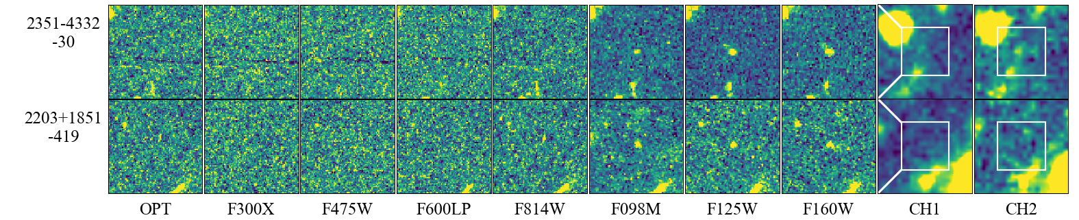
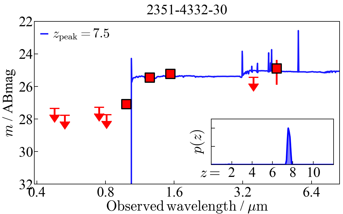
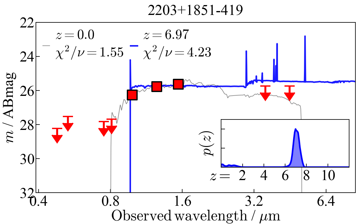
Figure 14: Same as Fig. 13 but for two source candidates selected in the z6 selection. Clean non-detection in the optical filters and tentative/non-detection in the two IRAC bands make the photometric redshift strongly peaked at $z\,\hbox to0.0pt{\lower 3.5pt\hbox{$\mathchar 0\relax\sim$}\hss}\raise 1.0pt\hbox{$>$}\,7$. sBoRG-2203+1851-419 has a point-source morphology; SED fitting analysis with a set of dwarf templates indicates that the object is more likely a foreground brown dwarf (gray solid line). The analysis with the dwarf templates is not reflected in the probability distribution inset.

5.2.5 Caveats on High-$z$ Source Color Selection

Redshift distributions for the color selections above are shown in Fig. 12. These selection functions are estimated in a completeness simulation in the same manner as in Morishita et al. (2018). It is noted that the shape of each selection function may slightly be changed depending on the depth of filters used for the selection, while the purpose here is to provide an approximate redshift range for each color selection. A dedicated study will provide completeness and contamination rates of high-$z$ source candidates (Leethochawalit, in prep.).

There are two caveats that interested readers may consider: besides the color cuts, combining photometric redshift results can improve the selection and exclude low-$z$ interlopers. For example, Morishita et al. (2018) only selected those with probability distribution at $z<6.5$ smaller than $30\%$, effectively excluding suspicious candidates. However, it is also noted that having too stringent conditions could exclude genuine high-$z$ galaxies with e.g., a moderate amount of dust, as their SEDs are impossible to distinguish from those of low-$z$ interlopers with the filter sets used here, leading to an incomplete high-$z$ candidate list. The other note is that selected candidates may still need visual inspection, to exclude contaminations such as stellar spikes, false detection of noise at the edge of images, false non-detection images i.e. those falling in the detector gap of WCF3-UVIS and ACS (whereas such a gap does not exist in the WFC3-IR channel). Lastly, the color selection criteria presented below are not exclusive of each other, and may be classified in more than one selection, as shown in Fig.12. Such duplication of redshift range is inevitable for more complete candidate selection with a dataset like SuperBoRG, where multiple filter configurations are available.

5.3 Example of Selected High-$z$ Candidates

As a demonstration of high-$z$ source selection and analysis, we here present newly identified source candidates from two programs, COS-GTO and CLASH, from 22 and 44 fields, respectively. These fields only allow the z10, z8_Y098, and z6 selections, while identified sources by the z8_Y098 selection were initially presented in Bradley et al. (2012) and Schmidt et al. (2014b). We therefore focus on the z10 selection and z6 selection in this study, as the purpose is to demonstrate how the actual selection proceeds as well as to provide a few caveats. For the rest of the high-$z$ source candidates selected from the entire SuperBoRG fields, and for comparison with the previously identified sources, readers are referred to a forthcoming paper (Roberts-Borsani, in prep.).

After applying the z10 selection above and $p_{\rm high}>0.7$ (see Table 3), we found 59 sources. Most of the sources (54) are from the CLASH program. However, our visually inspection found a significantly high contamination fraction, where only three of them are found as possible high-$z$ sources; the rest are either stellar spikes, noise structures at the edge of the detectors, or sources with suspicious non-detection where positive pixels are observed near the position in the optical images. This high contamination fraction in the CLASH fields is attributed to a relatively small number of available filters ($3$), while this is not the case for the COS-GTO data or other previous BoRG fields (e.g., Calvi et al., 2016; Morishita et al., 2018).

Two of the three possible candidates have significant IRAC ch1 detection, with F160W$-[3.6]>1.4$, which are rejected by an additional criterion for the z10 selection. The other one, sBoRG-0416-2403-398, does not have ch1 coverage but ch2, and is detected at $S/N=6.4$. While the color is still red (F160W$-[4.5]=1.8$), this does not immediately exclude the object from the z10 list (Fig. 13).

We check availability of other IR filters. A moderately deep $K_{S}$-band image taken with VISTA/VIRCAM is available (PID:198.A-2008, PI. Nonino, M.). We do not find any detection at the position of sBoRG-0416-2403-398, and thus we place an upper limit listed in the ESO-archive ($K_{S}=22.34$ ABmag, $5\sigma$). Placing this upper limit does not change the result, and its redshift probability distribution still peaks at $z\sim 10$.

Given the cosmic time at the inferred redshift, it is unlikely that this object has a very mature population of this color, implying a moderate amount of dust in the system is needed; such examples are seen in recent observations by ALMA (Watson et al., 2015; Laporte et al., 2017; Tamura et al., 2018). We fit the observed data points with a bayesian SED fitting code, gsf (Morishita et al., 2019) with a setup of fsps (Conroy et al., 2009) stellar population templates of solar metallicity, Chabrier (2003) IMF, and Calzetti et al. (2000) dust attenuation while fixing redshift to $z=10.4$, and the best-fit result infers $A_{V}=1.4_{-0.3}^{+0.2}$, with $\log M_{*}/M_{\odot}=10.0_{-0.3}^{+0.8}$.

On the other hand, because of the significant ch2 flux, the source also has a secondary redshift peak at $z\sim 3$. The total probability of a lower redshift ($z<6$) solution is $\sim 23\%$. To better constrain its SED and photometric redshift, additional photometric data points at $\sim 2\,\mu{\rm m}$ to $\sim 4\,\mu{\rm m}$ are desired, while spectroscopic follow-up of rest-frame UV emission lines would be challenging from the current ground facilities given its apparent magnitude.

Three fields in the COS-GTO program allow the z6 selection. Three sources are identified by the z6 selection criteria, one of which is rejected by visual inspection for possible flux contaminations in the non-detection images. The other two candidates have a sufficient number of filters (Fig. 14), including two IRAC bands, that constrains their photometric redshift well. sBoRG-2351-4332-30 has a striking color break ($\mathrm{F098M-F125W}=1.6$), making its redshift probability peak at $z\sim 7.5$. We see clean non-detection in the 4 optical filters. Its IRAC ch2 image detects moderate flux ($24.9\pm 0.6$ mag) without being significantly contaminated by neighboring objects while there is no detection in ch1. The object has a flat UV slope, effectively eliminating any significant possibility as a low-$z$ interloper ($<1\%$).

The other z6 candidate, sBoRG-2203+1851-419, also has clean non-detection in the optical bands. Fluxes are not detected in moderately deep IRAC images, placing upper limits to its SED. In combination with a flat $J_{125}-H_{160}$ color and the IRAC non-detection, the object has a small probability as a low-$z$ interloper ($\sim 12\%$).

Furthermore, the object is characterized by a compact morphology, and indeed satisfies the criteria for point-source selection defined by Eq. 1 in Section 4.3. Such high-$z$ sources with point-source morphologies are of particular interest, with regard to their possibility as low-luminosity quasars or compact starburst galaxies. Morishita et al. (2020) identified three candidates by the z8_Y105 selection and investigated their properties.

We repeat the photometric analysis for sBoRG-2203+1851-419 but this time with a set of dwarf templates taken from the IRTF spectral Library (Rayner et al., 2003), in the same way as in Morishita et al. (2020). The best-fit result provides a considerably smaller reduced-$\chi^{2}$ value (1.6 cf. 4.23 with extragalactic templates; see Fig. 13). This is not a surprise given a considerably high fraction of contaminating cool stars at this redshift, in contrast to the one at $z\,\hbox to0.0pt{\lower 3.5pt\hbox{$\mathchar 0\relax\sim$}\hss}\raise 1.0pt\hbox{$>$}\,8$ (e.g., Fig. 4 of Morishita et al., 2020). We therefore conclude this object is a foreground star. The sources presented here are summarized in Table 2.

6 Output products

As output products, we provide three separate catalogs — a master catalog that contains basic source properties such as coordinates, extraction flag, and structural parameters measured by SExtractor (Table 4), a flux catalog that lists flux measurements (Table 5), and a redshift catalog that contains spectroscopic and photometric redshifts, absolute UV magnitude ($M_{\rm UV}$) and rest-frame colors calculated with the best-fit SED (Table 6). All catalogs contain common objects that are brighter than the $3\sigma$ limiting magnitude in F160W of each field ($N=463662$). The columns included in the catalogs are summarized in Table 3 with brief descriptions. The extraction flag in the master catalog is derived by SExtractor, a sum of powers of 2 coded in decimal. For example, the flag can be used to check if a source has flux contamination from neighboring sources ($+1$), is de-blended from neighboring sources ($+2$), or is saturated ($+4$). Photometric flux measurements listed in the flux catalog are corrected for the RMS scaling (Sec. 3.1.3) and dust attenuation (Sec. 4.1), and scaled so they have a common magnitude zeropoint $m_{0}$ of 25 i.e. $m=-2.5\log f+m_{0}$ ABmag.

HST imaging data reduced in this study will be released with the final pixel scale of $0.\!^{\prime\prime}08$, which include co-added science frames, scaled RMS maps, and segmentation map, for all fields.

These catalogs, reduced imaging data (DOI: 10.17909/t9-m7tx-qb86), and SExtractor parameter files used for the flux measurement will be available via the dedicated site and the Mikulski Archive for Space Telescopes (MAST).

7 Summary

In this study, we introduced a new archival project, SuperBoRG, which collects previous HST parallel imaging data taken for extragalactic science cases, including pure-parallel (BoRG, HIPPIES, and COS-GTO) and coordinated-parallel programs (CLASH and RELICS). The final data set consists of the total number of 316 independent sightlines, reaching the total effective area of $\sim$ $0.41\,\mathrm{deg}^{2}$, which is the largest-area extragalactic survey with HST for extragalactic science. We reduced these datasets in a consistent way, with an updated version of our customized pipeline. We showed that our new sky background subtraction step improves the limiting magnitude by $\sim 0.1$ mag, detecting a few hundreds more faint sources at $\sim 27$ mag per field. We also showed that our revise in the photometric flux extraction method, from previous isophotal to aperture, can minimize possible false identification of low-$z$ sources as high-$z$ source candidates.

We presented photometric analyses, including photometric redshift analysis and color selection of high-$z$ source candidates by means of the Lyman break technique. In the last section, we presented newly identified luminous source candidates at $z\,\hbox to0.0pt{\lower 3.5pt\hbox{$\mathchar 0\relax\sim$}\hss}\raise 1.0pt\hbox{$>$}\,7$ from the fields of two programs as a preliminary result. One of them has a primary redshift peak at $z\sim 10.4$, though its strong detection in IRAC ch2 suggests that this may be a low-$z$ dusty galaxy ($\sim 23\%$). The other two candidates have a strong redshift peak $z\sim 7$, while one of them has a point-source morphology; phot-$z$ analysis with a set of dwarf templates indeed inferred that this object is more likely a foreground star. A complete list and further analysis of high-$z$ source candidates from the entire SuperBoRG fields will be presented in a forthcoming paper.

While the primary focus of SuperBoRG is on luminous source candidates at high redshift, the dataset is also suitable for science cases at low and intermediate redshifts, especially in fields with supplemental data from follow-up HST and Spitzer observations. The imaging data products and catalogs will be publicly available.

Table 1:

Field	Survey	R.A.	Decl.	F350LP	F600LP	F606W	F814W	F098M	F105W	F125W	F140W	F160W	IRAC1	IRAC2
		deg	deg	mag	mag	mag	mag	mag	mag	mag	mag	mag	mag	mag
BoRG Cycle17
0540-6409	B17	8.488e+01	-6.415e+01	—	—	26.88	—	26.54	—	26.49	—	26.17	—	—
0553-6405	B17	8.827e+01	-6.409e+01	—	—	27.04	—	26.78	—	26.66	—	26.24	23.29	23.38
0624-6432	B17	9.590e+01	-6.453e+01	—	—	27.03	—	26.26	—	26.23	—	25.64	—	—
0624-6440	B17	9.595e+01	-6.466e+01	—	—	26.86	—	26.57	—	26.37	—	25.90	—	23.34
0637-7518	B17	9.927e+01	-7.531e+01	—	—	27.12	—	26.74	—	26.51	—	25.88	23.62	23.27
0756+3043	B17	1.190e+02	3.072e+01	—	—	26.98	—	26.76	—	26.57	—	26.11	—	—
0808+3946	B17	1.221e+02	3.976e+01	—	—	26.82	—	26.57	—	26.47	—	25.94	23.45	23.00
0819+4911	B17	1.248e+02	4.918e+01	—	—	26.71	—	26.66	—	26.36	—	25.73	—	—
0820+2332	B17	1.250e+02	2.354e+01	—	—	26.89	—	26.51	—	26.09	—	25.84	—	—
0906+0255	B17	1.364e+02	2.926e+00	—	—	27.08	—	26.94	—	26.90	—	26.48	23.95	23.24
0909+0002	B17	1.373e+02	-3.023e-02	—	—	28.25	—	27.95	—	27.79	—	26.94	23.69	23.40
0922+4505	B17	1.404e+02	4.509e+01	—	—	26.81	—	26.68	—	26.56	—	26.21	—	—
1031+3804	B17	1.577e+02	3.806e+01	—	—	26.65	—	26.37	—	26.27	25.30	25.96	24.17	23.31
1152+5441	B17	1.780e+02	5.468e+01	—	—	27.24	—	27.01	—	26.96	26.19	26.60	23.67	—
1153+0056	B17	1.782e+02	9.319e-01	—	—	27.02	—	26.76	—	26.72	—	26.33	24.17	23.35
1230+0750	B17	1.875e+02	7.826e+00	—	—	26.72	—	26.08	—	25.83	—	25.60	23.40	—
1245+3356	B17	1.912e+02	3.394e+01	—	—	26.88	—	26.78	—	26.63	—	26.06	24.07	23.53
1437+5043	B17	2.192e+02	5.072e+01	—	—	26.92	—	27.31	27.05	27.26	—	26.97	23.93	23.40
1632+3733	B17	2.481e+02	3.756e+01	—	—	27.01	—	26.89	—	26.83	25.67	26.45	23.73	23.32
1632+3737	B17	2.479e+02	3.761e+01	28.00	—	26.74	—	26.80	27.38	27.33	27.42	27.12	23.67	23.34
BoRG Cycle19
0456-2203	B19	7.396e+01	-2.205e+01	—	—	27.02	—	26.71	—	26.64	24.89	26.36	23.78	23.30
0951+3304	B19	1.477e+02	3.307e+01	—	—	26.66	—	26.47	—	26.40	—	26.15	24.00	23.21
0952+5304	B19	1.479e+02	5.307e+01	—	—	27.02	—	26.68	—	26.72	—	26.44	—	—
1059+0519	B19	1.647e+02	5.312e+00	—	—	26.79	—	26.70	—	26.65	—	26.40	24.02	23.28
…	…	…	…	…	…	…	…	…	…	…	…	…	…	…
0722+0729	REL	1.105e+02	7.484e+00	26.30	—	—	—	—	26.22	26.12	26.11	25.98	—	—
0830+6555	REL	1.276e+02	6.591e+01	26.75	—	—	—	—	26.44	26.47	26.67	26.26	23.50	23.21
0843+3627	REL	1.307e+02	3.646e+01	26.02	—	—	—	—	26.21	26.26	26.20	26.10	23.86	23.38
1132-1950	REL	1.729e+02	-1.983e+01	26.73	—	—	—	—	26.52	26.30	26.34	26.24	23.81	23.63
1335+4054	REL	2.038e+02	4.090e+01	26.99	—	—	—	—	26.75	26.43	26.52	26.40	24.18	24.36
1515-1517	REL	2.287e+02	-1.528e+01	26.61	—	—	—	—	26.42	26.24	26.30	26.15	23.32	23.04
1521-8134	REL	2.302e+02	-8.157e+01	26.77	—	—	—	—	26.39	26.52	26.59	26.30	23.23	23.27
1917-3335	REL	2.894e+02	-3.359e+01	26.66	—	—	—	—	26.42	26.27	26.31	26.13	—	—
2212-0354	REL	3.330e+02	-3.903e+00	26.81	—	—	—	—	26.45	26.30	26.29	26.19	23.82	23.82

Note. — Example of the field table, listing coordinates and $5\,\sigma$-limiting magnitudes of filters. The full table is available online.

Table 2: Photometric properties of high-$z$ source candidates identified in the CLASH and COS-GTO fields.

Field ID	Survey	ObjID	R.A.	Decl.	$z_{\rm peak}$	$M_{\rm UV}$	$r$	$m_{160}$	$\chi^{2}/\nu$	${\chi^{2}/\nu}_{\rm dw}$
			deg	deg		mag	kpc	mag
z10 selection
sBoRG-0416-2403	clash	398	63.923630	-24.034565	10.4	-21.9	0.80	25.7	0.10	15.02
z6 selection
sBoRG-2351-4332	cosgto	30	357.644440	-43.542427	7.55	-21.7	0.98	25.2	3.60	9.32
sBoRG-2203+1851†	cosgto	419	330.706510	18.847076	6.97	-21.3	1.03	25.6	4.23	1.55

Table 3: Columns and description for the photometric catalogs.

Column name	Units	Description
Master catalog
field		BoRG field name.
survey		Survey name. Bxx: BoRG cyclexx. Hxx: HIPPIES cyclexx. CLA: CLASH. REL: RELICS. COS: COS-GTO.
id		Individual identification name of objects.
ra	degree	R.A. (J2000).
dec	degree	Declination (J2000).
x	pixel	x position in image coordinate.
y	pixel	y position in image coordinate.
kron_radius	pixel	Kron radius measured by SExtractor.
a_image	pixel	Radius along the major axis measured by SExtractor.
b_image	pixel	Radius along the minor axis measured by SExtractor.
theta	degree	Position angle measured by SExtractor.
class_star		Class star indicator measured by SExtractor.
flux_radius	pixel	Non-parametric half-light radius measured by SExtractor.
flags		Extraction flag from SExtractor.
f_persist		Flag for IR-image persistence at object positions. 0: Clean, 1: Contaminated.
flag_detect		Flag for source detection in F160W images. 0: $S/N<3$, 1: $S/N>3$.
flux_ratio0		Flux concentration ratio $f_{0}/f_{1}$, where $f_{0}$ ($f_{1}$) is flux measured in an aperture of diameter size $2$ (4) pixels.
flux_ratio1		Flux concentration ratio $f_{1}/f_{2}$, where $f_{1}$ ($f_{2}$) is flux measured in an aperture of diameter size $4$ (8) pixels.
flux_scale		Scale ratio of total flux to aperture flux measured in F160W. For those with scale $<1$, scale is set to 1.
faper_F160W	$f_{\nu}$	Aperture flux in F160W, with diameter size of 8 pixels.
eaper_F160W	$f_{\nu}$	Flux error of faper_F160W.
faper_F140W	$f_{\nu}$	Aperture flux in F140W, with diameter size of 8 pixels.
eaper_F140W	$f_{\nu}$	Flux error of faper_F140W.
Flux catalog
f_xx	$f_{\nu}$	Total flux of objects in band xx.
e_xx	$f_{\nu}$	Flux error ($1\sigma$) in total flux of objects in band xx.
flag_xx		Extraction flag for IRAC photometry by tphot. IRAC bands (channels 1 to 4) only.
fiso_xx	$f_{\nu}$	Isophotal flux of objects in band xx.
eiso_xx	$f_{\nu}$	Isophotal flux error ($1\sigma$) in total flux of objects in band xx.
Redshift catalog
zspec		Spectroscopic redshift, if available.
flag_zspec		Spectroscopic redshift quality flag. $2$: LIKELY ($\sim 80\%$ reliability), $3$: SECURE ($\sim 100\%$), $9$: SINGLE-LINE ($>90\%$).
z16		Photometric redshift at the 16th percentile of redshift distribution.
z50		Photometric redshift at the 50th percentile of redshift distribution.
z84		Photometric redshift at the 84th percentile of redshift distribution.
zpeak		Photometric redshift at the peak of redshift distribution.
MUV16	mag	Absolute UV (1450 Å) magnitude calculated at z16.
MUV50	mag	Absolute UV (1450 Å) magnitude calculated at z50.
MUV84	mag	Absolute UV (1450 Å) magnitude calculated at z84.
MUVpeak	mag	Absolute UV (1450 Å) magnitude calculated at zpeak.
zset		A limit redshift for the calculation of plow and phigh.
plow		Total probability of redshift distribution at $z<{\rm zset}$.
phigh		Total probability of redshift distribution at $z>{\rm zset}$.
UVbeta_lambda		UV-beta slope ($\beta_{\lambda}$) calculated with the best-fit template at zpeak.
U-V	mag	Rest-frame $U-V$ color calculated with the best-fit template at zpeak.
B-V	mag	Rest-frame $B-V$ color calculated with the best-fit template at zpeak.
V-J	mag	Rest-frame $V-J$ color calculated with the best-fit template at zpeak.
z-J	mag	Rest-frame $z-J$ color calculated with the best-fit template at zpeak.
chi2		Reduced chi-square at zpeak.
zmc		Photometric redshift derived with the posterior distribution.
nfilt		Number of filters used for photometric redshift fit.

Note. — All fluxes are corrected for the Galactic dust extinction, and set to magnitude zeropoint of $m_{0}=25$ i.e. $m=-2.5\log({\rm flux})+m_{0}$. For sources with filters without data coverage (including those falling in the UVIS detector gap), the flux error arrays are set to $-99$.

=0.5in

Table 4:

field	survey	id	ra	dec	x	y	kron_radius	a_image	b_image	theta	class_star	flux_radius	flags	f_persist	flag_detect	flux_ratio0	flux_ratio1	flux_scale	faper_F160W	eaper_F160W	faper_F140W	eaper_F140W
0624-6432	B17	692	95.86369	-64.52982	1785.8214	1078.0853	3.500	1.839	1.717	9.887	0.976	2.000	0	0	1	0.421	0.563	1.117	4.752	0.115	4.792	0.068
0624-6432	B17	693	95.871475	-64.529785	1635.2957	1079.6268	6.707	1.428	1.261	-42.633	0.379	2.944	0	0	1	0.298	0.440	1.531	0.767	1.018	0.628	1.015
0624-6432	B17	694	95.876686	-64.52985	1534.4542	1077.1658	5.278	2.458	1.239	-55.542	0.425	3.372	0	0	1	0.304	0.490	1.720	0.969	0.234	0.643	0.069
0624-6432	B17	695	95.88714	-64.529335	1332.1267	1100.2076	3.994	1.283	1.026	-42.011	0.452	1.565	0	0	1	0.339	0.707	1.091	0.489	0.112	0.382	0.066
0624-6432	B17	696	95.85694	-64.529915	1916.4974	1073.7604	5.134	2.476	1.288	-36.673	0.437	3.159	0	0	1	0.344	0.389	1.517	1.084	0.256	0.884	0.129
0624-6432	B17	697	95.88604	-64.52994	1353.4473	1073.0458	4.331	2.216	1.712	-84.916	0.560	3.178	0	0	1	0.303	0.397	1.571	1.612	0.112	1.545	0.066
0624-6432	B17	698	95.91055	-64.52986	879.05133	1076.2301	3.500	0.932	0.749	88.795	0.369	1.728	0	0	1	0.306	0.668	1.065	0.390	0.248	0.013	0.067
0624-6432	B17	699	95.9241	-64.5299	616.85004	1074.6774	3.500	1.539	1.437	83.791	0.119	1.853	0	0	1	0.354	0.594	1.068	1.630	0.110	1.706	0.065
0624-6432	B17	700	95.86257	-64.52992	1807.6199	1073.5538	3.500	1.832	1.494	-21.711	0.923	1.727	0	0	1	0.450	0.626	1.087	2.620	0.114	3.050	0.067
0624-6432	B17	701	95.872406	-64.52989	1617.3138	1075.0374	5.676	1.165	0.947	-60.002	0.414	1.843	0	0	1	0.309	0.584	1.105	0.432	0.137	0.010	0.077
0624-6432	B17	702	95.88535	-64.52991	1366.6926	1074.1544	6.775	1.416	0.989	86.399	0.351	3.004	0	0	1	0.264	0.385	1.499	0.532	0.112	0.418	0.067
0624-6432	B17	703	95.87326	-64.52997	1600.6573	1071.4878	3.500	1.888	1.687	-73.838	0.982	2.056	0	0	1	0.391	0.555	1.156	2.944	0.208	2.969	0.082
0624-6432	B17	704	95.8551	-64.529915	1952.1763	1073.8175	6.801	1.110	0.775	2.004	0.368	2.387	0	0	1	0.385	0.549	1.217	0.490	0.121	0.464	0.088
0624-6432	B17	705	95.93543	-64.52996	397.5872	1071.7129	6.042	1.946	1.460	5.871	0.396	3.622	0	0	1	0.287	0.413	1.840	1.017	0.145	0.974	0.101
0624-6432	B17	706	95.85896	-64.530045	1877.3486	1067.7806	3.500	1.772	1.712	76.289	0.976	1.847	0	0	1	0.406	0.594	1.096	7.224	0.113	8.520	0.068
0624-6432	B17	707	95.902954	-64.52934	1026.032	1099.8868	7.204	1.446	0.778	39.550	0.348	2.645	0	0	1	0.303	0.373	1.212	0.488	0.116	0.348	0.067
0624-6432	B17	708	95.87867	-64.530106	1495.9816	1065.265	4.298	1.891	1.555	57.190	0.958	2.140	0	0	1	0.341	0.558	1.196	2.823	0.114	2.962	0.067
0624-6432	B17	709	95.911705	-64.53009	856.7665	1066.0654	3.500	1.378	1.289	-80.727	0.013	1.873	0	0	1	0.284	0.569	1.033	1.037	0.127	0.910	0.068
0624-6432	B17	710	95.90576	-64.53012	971.83105	1064.6478	3.500	1.329	0.992	-48.639	0.448	1.772	0	0	1	0.422	0.567	1.004	0.499	0.112	0.508	0.066
0624-6432	B17	711	95.85113	-64.53013	2029.095	1064.1027	3.918	1.254	1.156	-67.490	0.352	2.448	0	0	1	0.202	0.371	1.091	0.588	0.119	0.210	0.071
0624-6432	B17	712	95.89998	-64.53	1083.6361	1070.3765	4.686	1.537	1.361	-70.912	0.862	2.002	0	0	1	0.280	0.563	1.129	1.603	0.110	1.332	0.066
0624-6432	B17	713	95.87182	-64.53016	1628.6356	1062.8197	3.943	1.475	0.914	-69.848	0.396	1.830	0	0	1	0.330	0.605	1.111	0.543	0.114	-0.022	0.068
0624-6432	B17	714	95.919334	-64.53017	709.16614	1062.4702	5.654	1.011	0.949	-60.457	0.548	1.517	0	0	1	0.329	0.666	1.021	0.398	0.193	0.353	0.073
0624-6432	B17	715	95.88368	-64.53023	1398.968	1059.8787	4.491	1.063	1.009	-4.259	0.451	1.908	0	0	1	0.261	0.534	1.000	0.491	0.112	0.405	0.087
0624-6432	B17	716	95.852745	-64.53028	1997.6974	1057.1389	5.990	1.244	1.089	36.919	0.463	2.739	0	0	1	0.348	0.451	1.393	0.564	0.116	0.311	0.069
0624-6432	B17	717	95.90474	-64.53029	991.6068	1057.0814	6.129	1.158	1.015	-69.227	0.359	2.414	2	0	1	0.284	0.452	1.200	0.498	0.108	0.400	0.065
0624-6432	B17	718	95.87924	-64.53039	1485.0106	1052.5944	6.526	2.423	1.591	51.264	0.516	5.886	0	0	1	0.281	0.405	2.645	1.341	0.113	1.187	0.066
0624-6432	B17	719	95.910225	-64.530334	885.33154	1055.2196	3.604	1.306	0.819	60.341	0.417	1.865	0	0	1	0.379	0.582	1.063	0.445	0.112	0.393	0.066
0624-6432	B17	720	95.91241	-64.53033	843.1588	1055.3024	5.104	0.922	0.676	-70.220	0.425	1.552	0	0	1	0.398	0.730	1.074	0.330	0.112	0.013	0.066
0624-6432	B17	721	95.92927	-64.53034	516.8863	1054.5538	4.604	1.266	0.959	-33.048	0.716	1.867	0	0	1	0.325	0.684	1.230	0.781	0.381	0.794	0.189

Note. — Example 30 lines of the master catalog. The full table is available online.

=0.5in

Table 5:

field	survey	id	f_F300X	e_F300X	f_F350LP	e_F350LP	f_F435W	e_F435W	…	f_F125W	e_F125W	f_F140W	e_F140W	f_F160W	e_F160W	f_irac1	e_irac1	f_irac2	e_irac2	f_irac3	e_irac3	f_irac4	e_irac4	flag_irac1	flag_irac2	flag_irac3	flag_irac4
1301+1300	B25	1	0.000	-99.000	3.920	1.272	0.000	-99.000	…	19.766	1.627	22.364	1.486	25.674	1.860	0.000	-99.000	0.000	-99.000	0.000	-99.000	0.000	-99.000	0	0	0	0
1301+1300	B25	2	0.000	-99.000	1.017	0.084	0.000	-99.000	…	0.944	5.237	0.880	10.597	1.226	4.983	0.000	-99.000	0.000	-99.000	0.000	-99.000	0.000	-99.000	0	0	0	0
1301+1300	B25	3	0.000	-99.000	12.852	0.108	0.000	-99.000	…	75.957	0.119	90.714	0.111	106.165	0.140	0.000	-99.000	0.000	-99.000	0.000	-99.000	0.000	-99.000	0	0	0	0
1301+1300	B25	4	0.000	-99.000	1.068	0.060	0.000	-99.000	…	0.752	25.984	0.952	24.338	0.963	26.682	0.000	-99.000	0.000	-99.000	0.000	-99.000	0.000	-99.000	0	0	0	0
1301+1300	B25	5	0.000	-99.000	0.223	0.067	0.000	-99.000	…	0.587	0.109	0.476	0.098	0.499	0.109	24.253	1.619	0.000	-99.000	0.000	-99.000	0.000	-99.000	0	0	0	0
1301+1300	B25	6	0.000	-99.000	0.162	0.079	0.000	-99.000	…	0.361	8.465	0.393	10.226	0.364	9.321	0.000	-99.000	0.000	-99.000	0.000	-99.000	0.000	-99.000	0	0	0	0
1301+1300	B25	7	0.000	-99.000	0.087	0.072	0.000	-99.000	…	0.650	0.098	0.697	0.089	0.802	0.110	0.000	-99.000	0.000	-99.000	0.000	-99.000	0.000	-99.000	0	0	0	0
1301+1300	B25	8	0.000	-99.000	9.506	0.087	0.000	-99.000	…	50.462	0.096	59.563	0.088	68.997	0.112	0.000	-99.000	0.000	-99.000	0.000	-99.000	0.000	-99.000	0	0	0	0
1301+1300	B25	9	0.000	-99.000	0.458	0.280	0.000	-99.000	…	1.503	0.433	1.900	0.412	1.818	0.475	0.000	-99.000	0.000	-99.000	0.000	-99.000	0.000	-99.000	0	0	0	0
1301+1300	B25	10	0.000	-99.000	0.526	0.065	0.000	-99.000	…	0.619	0.068	0.750	0.063	1.287	0.080	0.000	-99.000	0.000	-99.000	0.000	-99.000	0.000	-99.000	0	0	0	0
1301+1300	B25	11	0.000	-99.000	0.072	0.088	0.000	-99.000	…	0.117	0.131	0.217	0.117	0.210	0.143	0.000	-99.000	0.000	-99.000	0.000	-99.000	0.000	-99.000	0	0	0	0
1301+1300	B25	12	0.000	-99.000	0.555	0.144	0.000	-99.000	…	1.441	0.260	1.589	0.492	2.015	0.240	0.000	-99.000	0.000	-99.000	0.000	-99.000	0.000	-99.000	0	0	0	0
1301+1300	B25	13	0.000	-99.000	0.126	0.041	0.000	-99.000	…	0.114	0.045	0.097	0.042	0.034	0.053	0.000	-99.000	0.000	-99.000	0.000	-99.000	0.000	-99.000	0	0	0	0
1301+1300	B25	14	0.000	-99.000	0.167	0.059	0.000	-99.000	…	0.242	0.072	0.246	0.066	0.267	0.082	4.463	1.659	0.000	-99.000	0.000	-99.000	0.000	-99.000	0	0	0	0
1301+1300	B25	15	0.000	-99.000	2.793	0.124	0.000	-99.000	…	6.383	0.181	6.958	0.158	7.284	0.221	0.000	-99.000	0.000	-99.000	0.000	-99.000	0.000	-99.000	0	0	0	0
1301+1300	B25	16	0.000	-99.000	0.666	0.151	0.000	-99.000	…	0.728	0.160	0.733	0.148	0.574	0.188	0.000	-99.000	0.000	-99.000	0.000	-99.000	0.000	-99.000	0	0	0	0
1301+1300	B25	17	0.000	-99.000	0.100	0.102	0.000	-99.000	…	0.140	0.111	0.329	0.102	0.167	0.130	0.000	-99.000	0.000	-99.000	0.000	-99.000	0.000	-99.000	0	0	0	0
1301+1300	B25	18	0.000	-99.000	0.104	0.040	0.000	-99.000	…	0.101	0.044	0.120	0.041	0.158	0.052	0.000	-99.000	0.000	-99.000	0.000	-99.000	0.000	-99.000	0	0	0	0
1301+1300	B25	19	0.000	-99.000	0.317	0.050	0.000	-99.000	…	0.418	0.122	0.454	0.060	0.448	0.098	0.000	-99.000	0.000	-99.000	0.000	-99.000	0.000	-99.000	0	0	0	0
1301+1300	B25	20	0.000	-99.000	0.101	0.166	0.000	-99.000	…	0.110	0.227	0.292	0.206	0.219	0.255	4.771	1.622	0.000	-99.000	0.000	-99.000	0.000	-99.000	2	0	0	0
1301+1300	B25	21	0.000	-99.000	0.015	0.041	0.000	-99.000	…	0.116	0.045	0.104	0.042	0.057	0.053	0.000	-99.000	0.000	-99.000	0.000	-99.000	0.000	-99.000	0	0	0	0
1301+1300	B25	22	0.000	-99.000	3.828	0.140	0.000	-99.000	…	5.259	0.188	5.219	0.172	5.499	0.212	0.000	-99.000	0.000	-99.000	0.000	-99.000	0.000	-99.000	0	0	0	0
1301+1300	B25	23	0.000	-99.000	-0.019	0.040	0.000	-99.000	…	0.122	0.048	0.112	0.048	0.078	0.056	0.000	-99.000	0.000	-99.000	0.000	-99.000	0.000	-99.000	0	0	0	0
1301+1300	B25	24	0.000	-99.000	0.143	0.051	0.000	-99.000	…	0.023	0.057	0.043	0.053	0.195	0.067	0.000	-99.000	0.000	-99.000	0.000	-99.000	0.000	-99.000	0	0	0	0
1301+1300	B25	25	0.000	-99.000	0.029	0.057	0.000	-99.000	…	0.166	0.063	0.264	0.058	0.185	0.073	0.000	-99.000	0.000	-99.000	0.000	-99.000	0.000	-99.000	0	0	0	0
1301+1300	B25	26	0.000	-99.000	28.192	0.051	0.000	-99.000	…	40.712	0.053	42.117	0.049	42.048	0.063	4.303	1.621	0.000	-99.000	0.000	-99.000	0.000	-99.000	0	0	0	0
1301+1300	B25	27	0.000	-99.000	0.044	0.040	0.000	-99.000	…	0.030	0.045	0.109	0.041	0.107	0.053	0.000	-99.000	0.000	-99.000	0.000	-99.000	0.000	-99.000	0	0	0	0
1301+1300	B25	28	0.000	-99.000	-0.010	0.045	0.000	-99.000	…	-0.011	0.057	0.070	0.052	0.111	0.065	8.442	1.684	0.000	-99.000	0.000	-99.000	0.000	-99.000	0	0	0	0
1301+1300	B25	29	0.000	-99.000	0.173	0.055	0.000	-99.000	…	0.186	0.058	0.184	0.054	0.209	0.069	0.000	-99.000	0.000	-99.000	0.000	-99.000	0.000	-99.000	0	0	0	0
1301+1300	B25	30	0.000	-99.000	0.151	0.060	0.000	-99.000	…	0.117	0.113	0.112	0.180	0.215	0.107	11.230	1.649	0.000	-99.000	0.000	-99.000	0.000	-99.000	0	0	0	0

Note. — Example 30 lines of the photometric flux catalog. Middle columns are omitted to be fitted in the manuscript size. The full table is available online.

=0.0in

Table 6:

field	survey	id	zspec	flag_zspec	z16	z50	z84	zpeak	MUV16	MUV50	MUV84	MUVpeak	zset	plow	phigh	UVbeta_lambda	U-V	B-V	V-J	z-J	chi2	zmc	nfilt
1301+1300	B25	57	-99.0	-99.0	0.45	1.6	2.59	1.42	-14.014	-18.051	-19.691	-17.651	6.5	1.0	0.0	-2.278	-0.267	0.127	-0.631	-0.078	0.701	4.137	7
1301+1300	B25	58	-99.0	-99.0	0.36	2.28	2.39	2.29	-12.952	-18.837	-18.999	-18.852	6.5	1.0	0.0	-2.101	-0.012	0.132	-0.24	-0.004	2.783	2.354	7
1301+1300	B25	59	-99.0	-99.0	1.27	1.64	3.41	1.39	-16.541	-17.397	-19.9	-16.842	6.5	0.911	0.089	-2.556	-0.444	0.263	-1.311	-0.167	5.349	1.349	7
1301+1300	B25	60	-99.0	-99.0	0.9	3.94	9.97	0.01	-16.984	-21.969	-25.185	-5.622	6.5	0.651	0.349	-2.451	1.306	0.548	-1.644	-0.167	2.997	0.497	7
1301+1300	B25	61	-99.0	-99.0	0.84	1.14	1.38	1.27	-17.346	-18.337	-18.97	-18.694	6.5	1.0	0.0	-1.382	1.071	0.495	1.187	0.434	0.087	1.151	7
1301+1300	B25	62	-99.0	-99.0	0.38	1.35	3.86	0.39	-14.587	-18.545	-22.13	-14.661	6.5	1.0	0.0	-2.301	-0.195	0.214	-0.333	0.022	2.982	1.461	7
1301+1300	B25	63	-99.0	-99.0	0.89	2.59	7.0	1.34	-14.368	-17.942	-21.38	-15.709	6.5	0.81	0.19	-2.551	-0.054	0.462	0.167	0.18	1.777	0.368	7
1301+1300	B25	64	-99.0	-99.0	0.88	1.68	2.65	1.44	-16.78	-18.915	-20.469	-18.397	6.5	0.986	0.014	-2.555	-0.459	0.252	-1.299	-0.167	1.277	1.659	7
1301+1300	B25	65	-99.0	-99.0	1.32	5.28	7.91	1.39	-17.235	-21.979	-23.38	-17.407	6.5	0.614	0.385	-2.556	-0.444	0.263	-1.309	-0.166	5.218	5.612	7
1301+1300	B25	66	-99.0	-99.0	0.75	3.4	7.46	0.18	-8.875	-13.931	-16.652	-4.797	6.5	0.692	0.307	-0.517	2.287	1.083	2.204	0.694	0.652	2.404	7
1301+1300	B25	67	-99.0	-99.0	0.08	0.27	2.78	2.78	-9.981	-13.057	-20.423	-20.423	6.5	1.0	0.0	-2.553	-0.456	0.253	-1.295	-0.166	3.364	0.239	7
1301+1300	B25	68	-99.0	-99.0	0.33	2.33	3.22	2.78	-12.639	-18.844	-19.956	-19.45	6.5	1.0	0.0	-2.555	-0.457	0.253	-1.3	-0.166	1.536	3.525	7
1301+1300	B25	69	-99.0	-99.0	0.77	2.62	4.45	0.4	-15.308	-19.383	-21.211	-13.324	6.5	0.97	0.03	-2.5	-0.265	0.316	0.35	0.438	0.63	3.962	7
1301+1300	B25	70	-99.0	-99.0	0.4	1.64	3.71	3.57	-14.925	-19.389	-22.183	-22.05	6.5	1.0	0.0	-2.32	-0.122	0.275	-0.085	0.169	1.089	2.971	7
1301+1300	B25	71	-99.0	-99.0	1.35	4.58	9.2	0.39	-11.146	-15.322	-17.739	-7.262	6.5	0.653	0.346	0.9	1.263	0.676	1.872	0.666	4.044	5.127	7
1301+1300	B25	72	-99.0	-99.0	1.05	3.48	5.97	1.69	-14.603	-18.659	-20.528	-16.187	6.5	0.89	0.109	-2.553	-0.422	0.276	-1.322	-0.166	1.91	4.119	7
1301+1300	B25	73	-99.0	-99.0	2.54	10.05	11.35	10.74	-15.673	-20.43	-20.851	-20.66	6.5	0.272	0.728	-2.553	-0.436	0.266	-1.308	-0.165	1.235	10.784	7
1301+1300	B25	74	-99.0	-99.0	2.4	2.91	3.13	2.82	-20.06	-20.722	-20.973	-20.614	6.5	1.0	0.0	-2.554	-0.468	0.245	-1.289	-0.166	2.441	3.214	7
1301+1300	B25	75	-99.0	-99.0	2.2	9.64	10.99	10.51	-15.715	-20.82	-21.273	-21.119	6.5	0.317	0.682	-2.555	-0.44	0.265	-1.312	-0.166	4.164	2.412	7
1301+1300	B25	76	-99.0	-99.0	0.68	1.31	3.52	1.14	-17.405	-19.522	-22.888	-19.063	6.5	1.0	0.0	-1.946	0.335	0.114	0.527	0.248	0.198	3.631	7
1301+1300	B25	77	-99.0	-99.0	0.08	0.29	1.44	0.01	-10.652	-13.924	-18.857	-5.95	6.5	1.0	0.0	-2.346	1.487	0.655	0.79	0.672	7.415	1.832	7
1301+1300	B25	78	-99.0	-99.0	0.31	2.29	3.42	3.52	-12.636	-18.956	-20.335	-20.435	6.5	1.0	0.0	-2.555	-0.451	0.257	-1.304	-0.166	2.371	2.553	7
1301+1300	B25	79	-99.0	-99.0	0.67	2.59	4.2	1.15	-14.723	-19.195	-20.863	-16.455	6.5	0.994	0.006	-2.124	-0.098	0.061	-0.338	-0.048	0.375	3.022	7
1301+1300	B25	80	-99.0	-99.0	0.05	0.15	0.7	0.12	0.157	-2.477	-6.804	-1.921	6.5	1.0	0.0	8.633	2.27	1.024	1.211	0.265	3.927	0.107	7
1301+1300	B25	81	-99.0	-99.0	1.24	4.66	7.07	6.21	-13.482	-18.0	-19.445	-18.995	6.5	0.758	0.241	-1.961	0.166	0.002	-0.107	-0.031	0.139	2.506	7
1301+1300	B25	82	-99.0	-99.0	0.35	2.29	2.35	2.35	-14.934	-20.914	-21.002	-21.002	6.5	1.0	0.0	-2.184	-0.071	0.154	0.116	0.231	2.958	2.335	7
1301+1300	B25	83	-99.0	-99.0	1.95	8.3	9.96	9.64	-14.769	-19.767	-20.398	-20.285	6.5	0.363	0.637	-2.552	-0.457	0.251	-1.291	-0.165	0.293	8.409	7
1301+1300	B25	84	-99.0	-99.0	0.5	0.82	1.16	0.64	-17.134	-18.661	-19.786	-17.884	6.5	1.0	0.0	-1.977	0.779	0.574	0.701	0.085	5.098	1.232	7
1301+1300	B25	85	-99.0	-99.0	1.25	6.26	8.2	7.89	-14.113	-19.628	-20.564	-20.43	6.5	0.513	0.486	-2.555	-0.448	0.26	-1.307	-0.166	1.326	7.87	7
1301+1300	B25	86	-99.0	-99.0	0.4	0.51	3.57	0.45	-18.165	-18.879	-25.29	-18.508	6.5	1.0	0.0	-2.511	-0.272	0.333	0.08	0.4	2.068	0.43	7

Note. — Example 30 lines of the photometric redshift catalog. The full table is available online.

References

- Abramson et al. (2020) Abramson, L. E., Brammer, G. B., Schmidt, K. B., et al. 2020, MNRAS, 493, 952
- Anderson (2014) Anderson, J. 2014, The Impact of x-CTE in the WFC3/UVIS detector on Astrometry, Tech. rep.
- Annunziatella et al. (2016) Annunziatella, M., Mercurio, A., Biviano, A., et al. 2016, A&A, 585, A160
- Astropy Collaboration et al. (2013) Astropy Collaboration, Robitaille, T. P., Tollerud, E. J., et al. 2013, A&A, 558, A33
- Astropy Collaboration et al. (2018) Astropy Collaboration, Price-Whelan, A. M., SipHocz, B. M., et al. 2018, aj, 156, 123
- Atek et al. (2011) Atek, H., Siana, B., Scarlata, C., et al. 2011, ApJ, 743, 121
- Bañados et al. (2018) Bañados, E., Venemans, B. P., Mazzucchelli, C., et al. 2018, Nature, 553, 473
- Balestra et al. (2016) Balestra, I., Mercurio, A., Sartoris, B., et al. 2016, ApJS, 224, 33
- Becker et al. (2001) Becker, R. H., Fan, X., White, R. L., et al. 2001, AJ, 122, 2850
- Bernard et al. (2016) Bernard, S. R., Carrasco, D., Trenti, M., et al. 2016, ApJ, 827, 76
- Bertin & Arnouts (1996) Bertin, E., & Arnouts, S. 1996, A&AS, 117, 393
- Bhowmick et al. (2020) Bhowmick, A. K., Somerville, R. S., Di Matteo, T., et al. 2020, MNRAS, 496, 754
- Biviano et al. (2013) Biviano, A., Rosati, P., Balestra, I., et al. 2013, A&A, 558, A1
- Borncamp & Lim (2016) Borncamp, D., & Lim, P. L. 2016, Satellite Detection in Advanced Camera for Surveys/Wide Field Channel Images, Instrument Science Report ACS 2016-01
- Boucaud et al. (2016) Boucaud, A., Bocchio, M., Abergel, A., et al. 2016, A&A, 596, A63
- Bouwens et al. (2019) Bouwens, R. J., Stefanon, M., Oesch, P. A., et al. 2019, ApJ, 880, 25
- Bouwens et al. (2015) Bouwens, R. J., Illingworth, G. D., Oesch, P. A., et al. 2015, ApJ, 803, 34
- Bowler et al. (2020) Bowler, R. A. A., Jarvis, M. J., Dunlop, J. S., et al. 2020, MNRAS, 493, 2059
- Bowler et al. (2014) Bowler, R. A. A., Dunlop, J. S., McLure, R. J., et al. 2014, MNRAS, 440, 2810
- Bradač et al. (2014) Bradač, M., Ryan, R., Casertano, S., et al. 2014, ApJ, 785, 108
- Bradač et al. (2019) Bradač, M., Huang, K.-H., Fontana, A., et al. 2019, MNRAS, 489, 99
- Bradley et al. (2012) Bradley, L. D., Trenti, M., Oesch, P. A., et al. 2012, ApJ, 760, 108
- Brammer et al. (2008) Brammer, G. B., van Dokkum, P. G., & Coppi, P. 2008, ApJ, 686, 1503
- Bridge et al. (2019) Bridge, J. S., Holwerda, B. W., Stefanon, M., et al. 2019, ApJ, 882, 42
- Bruce et al. (2012) Bruce, V. A., Dunlop, J. S., Cirasuolo, M., et al. 2012, MNRAS, 427, 1666
- Calvi et al. (2016) Calvi, V., Trenti, M., Stiavelli, M., et al. 2016, ApJ, 817, 120
- Calzetti et al. (2000) Calzetti, D., Armus, L., Bohlin, R. C., et al. 2000, ApJ, 533, 682
- Cameron et al. (2019) Cameron, A. J., Trenti, M., Livermore, R. C., & van der Velden, C. 2019, MNRAS, 483, 1922
- Caminha et al. (2016) Caminha, G. B., Grillo, C., Rosati, P., et al. 2016, A&A, 587, A80
- Canny (1986) Canny, J. 1986, IEEE Transactions on Pattern Analysis and Machine Intelligence, PAMI-8, 679
- Cardelli et al. (1989) Cardelli, J. A., Clayton, G. C., & Mathis, J. S. 1989, ApJ, 345, 245
- Casertano et al. (2000) Casertano, S., de Mello, D., Dickinson, M., et al. 2000, AJ, 120, 2747
- Castellano et al. (2016) Castellano, M., Amorín, R., Merlin, E., et al. 2016, ArXiv e-prints, arXiv:1603.02461
- Cen & Haiman (2000) Cen, R., & Haiman, Z. 2000, ApJ, 542, L75
- Chabrier (2003) Chabrier, G. 2003, PASP, 115, 763
- Coe et al. (2006) Coe, D., Benítez, N., Sánchez, S. F., et al. 2006, AJ, 132, 926
- Coe et al. (2015) Coe, D., Bradley, L., & Zitrin, A. 2015, ApJ, 800, 84
- Coe et al. (2019) Coe, D., Salmon, B., Bradač, M., et al. 2019, ApJ, 884, 85
- Conroy et al. (2009) Conroy, C., Gunn, J. E., & White, M. 2009, ApJ, 699, 486
- Davies et al. (2018) Davies, F. B., Hennawi, J. F., Bañados, E., et al. 2018, ApJ, 864, 142
- Ellis et al. (2013) Ellis, R. S., McLure, R. J., Dunlop, J. S., et al. 2013, ApJ, 763, L7
- Finkelstein et al. (2013) Finkelstein, S. L., Papovich, C., Dickinson, M., et al. 2013, Nature, 502, 524
- Finkelstein et al. (2015) Finkelstein, S. L., Ryan, Jr., R. E., Papovich, C., et al. 2015, ApJ, 810, 71
- Foreman-Mackey et al. (2014) Foreman-Mackey, D., Sick, J., & Johnson, B. 2014, doi:10.5281/zenodo.12157
- Gaia Collaboration et al. (2018) Gaia Collaboration, Brown, A. G. A., Vallenari, A., et al. 2018, A&A, 616, A1
- Galamhos et al. (1999) Galamhos, C., Matas, J., & Kittler, J. 1999, in Proceedings. 1999 IEEE Computer Society Conference on Computer Vision and Pattern Recognition (Cat. No PR00149), Vol. 1, 554–560 Vol. 1
- Graur et al. (2014) Graur, O., Rodney, S. A., Maoz, D., et al. 2014, ApJ, 783, 28
- Grillo et al. (2015) Grillo, C., Suyu, S. H., Rosati, P., et al. 2015, ApJ, 800, 38
- Grogin et al. (2011) Grogin, N. A., Kocevski, D. D., Faber, S. M., et al. 2011, ApJS, 197, 35
- Gunn & Peterson (1965) Gunn, J. E., & Peterson, B. A. 1965, ApJ, 142, 1633
- Hack et al. (2012) Hack, W. J., Dencheva, N., Fruchter, A. S., et al. 2012, in American Astronomical Society Meeting Abstracts, Vol. 220, American Astronomical Society Meeting Abstracts #220, 135.15
- Hashimoto et al. (2018) Hashimoto, T., Laporte, N., Mawatari, K., et al. 2018, Nature, 557, 392
- Hinshaw et al. (2009) Hinshaw, G., Weiland, J. L., Hill, R. S., et al. 2009, ApJS, 180, 225
- Hoag et al. (2018) Hoag, A., Bradač, M., Brammer, G., et al. 2018, ApJ, 854, 39
- Hoag et al. (2019) Hoag, A., Bradač, M., Huang, K., et al. 2019, ApJ, 878, 12
- Holwerda et al. (2014) Holwerda, B. W., Trenti, M., Clarkson, W., et al. 2014, ApJ, 788, 77
- Illingworth et al. (2013) Illingworth, G. D., Magee, D., Oesch, P. A., et al. 2013, ApJS, 209, 6
- Karman et al. (2015) Karman, W., Caputi, K. I., Grillo, C., et al. 2015, A&A, 574, A11
- Karman et al. (2017) Karman, W., Caputi, K. I., Caminha, G. B., et al. 2017, A&A, 599, A28
- Koekemoer et al. (2011) Koekemoer, A. M., Faber, S. M., Ferguson, H. C., et al. 2011, ApJS, 197, 36
- Konno et al. (2014) Konno, A., Ouchi, M., Ono, Y., et al. 2014, ApJ, 797, 16
- Krist (1995) Krist, J. 1995, in Astronomical Society of the Pacific Conference Series, Vol. 77, Astronomical Data Analysis Software and Systems IV, ed. R. A. Shaw, H. E. Payne, & J. J. E. Hayes, 349
- Laporte et al. (2017) Laporte, N., Ellis, R. S., Boone, F., et al. 2017, ApJ, 837, L21
- Livermore et al. (2018) Livermore, R. C., Trenti, M., Bradley, L. D., et al. 2018, ApJ, 861, L17
- Lotz et al. (2017) Lotz, J. M., Koekemoer, A., Coe, D., et al. 2017, ApJ, 837, 97
- Madau et al. (1999) Madau, P., Haardt, F., & Rees, M. J. 1999, ApJ, 514, 648
- Makovoz & Marleau (2005) Makovoz, D., & Marleau, F. R. 2005, PASP, 117, 1113
- Mason & Gronke (2020) Mason, C. A., & Gronke, M. 2020, MNRAS, 499, 1395
- Mason et al. (2018a) Mason, C. A., Treu, T., Dijkstra, M., et al. 2018a, ApJ, 856, 2
- Mason et al. (2018b) Mason, C. A., Treu, T., de Barros, S., et al. 2018b, ApJ, 857, L11
- Matthee et al. (2018) Matthee, J., Sobral, D., Gronke, M., et al. 2018, A&A, 619, A136
- McLure et al. (2011) McLure, R. J., Dunlop, J. S., de Ravel, L., et al. 2011, MNRAS, 418, 2074
- Merlin et al. (2016) Merlin, E., Bourne, N., Castellano, M., et al. 2016, A&A, 595, A97
- Monna et al. (2017) Monna, A., Seitz, S., Balestra, I., et al. 2017, MNRAS, 466, 4094
- Morishita et al. (2014) Morishita, T., Ichikawa, T., & Kajisawa, M. 2014, ApJ, 785, 18
- Morishita et al. (2017) Morishita, T., Abramson, L. E., Treu, T., et al. 2017, ApJ, 835, 254
- Morishita et al. (2018) Morishita, T., Trenti, M., Stiavelli, M., et al. 2018, ApJ, 867, 150
- Morishita et al. (2019) Morishita, T., Abramson, L. E., Treu, T., et al. 2019, ApJ, 877, 141
- Morishita et al. (2020) Morishita, T., Stiavelli, M., Trenti, M., et al. 2020, arXiv e-prints, arXiv:2009.10078
- Mortlock et al. (2011) Mortlock, D. J., Warren, S. J., Venemans, B. P., et al. 2011, Nature, 474, 616
- Noeske et al. (2012) Noeske, K., Baggett, S., Bushouse, H., et al. 2012, WFC3 UVIS Charge Transfer Eciency October 2009 to October 2011, Tech. rep.
- Oesch et al. (2015) Oesch, P. A., van Dokkum, P. G., Illingworth, G. D., et al. 2015, ApJ, 804, L30
- Oesch et al. (2016) Oesch, P. A., Brammer, G., van Dokkum, P. G., et al. 2016, ApJ, 819, 129
- Oliphant (2006) Oliphant, T. E. 2006, A guide to NumPy, Vol. 1 (Trelgol Publishing USA)
- Ono et al. (2012) Ono, Y., Ouchi, M., Mobasher, B., et al. 2012, ApJ, 744, 83
- Peng et al. (2002) Peng, C. Y., Ho, L. C., Impey, C. D., & Rix, H.-W. 2002, AJ, 124, 266
- Peng et al. (2010) Peng, Y.-j., Lilly, S. J., Kovač, K., et al. 2010, ApJ, 721, 193
- Postman et al. (2012) Postman, M., Coe, D., Benítez, N., et al. 2012, ApJS, 199, 25
- Rayner et al. (2003) Rayner, J. T., Toomey, D. W., Onaka, P. M., et al. 2003, PASP, 115, 362
- Ren et al. (2020) Ren, K., Trenti, M., & Di Matteo, T. 2020, ApJ, 894, 124
- Riess et al. (2018) Riess, A. G., Rodney, S. A., Scolnic, D. M., et al. 2018, ApJ, 853, 126
- Roberts-Borsani et al. (2020) Roberts-Borsani, G. W., Ellis, R. S., & Laporte, N. 2020, MNRAS, arXiv:2002.02968
- Roberts-Borsani et al. (2016) Roberts-Borsani, G. W., Bouwens, R. J., Oesch, P. A., et al. 2016, ApJ, 823, 143
- Robertson (2010) Robertson, B. E. 2010, ApJ, 716, L229
- Robertson et al. (2015) Robertson, B. E., Ellis, R. S., Furlanetto, S. R., & Dunlop, J. S. 2015, ApJ, 802, L19
- Rojas-Ruiz et al. (2020) Rojas-Ruiz, S., Finkelstein, S. L., Bagley, M. B., et al. 2020, arXiv e-prints, arXiv:2002.06209
- Ryan et al. (2011) Ryan, R. E., Thorman, P. A., Yan, H., et al. 2011, ApJ, 739, 83
- Salmon et al. (2020) Salmon, B., Coe, D., Bradley, L., et al. 2020, ApJ, 889, 189
- Schlafly & Finkbeiner (2011) Schlafly, E. F., & Finkbeiner, D. P. 2011, ApJ, 737, 103
- Schlegel et al. (1998) Schlegel, D. J., Finkbeiner, D. P., & Davis, M. 1998, ApJ, 500, 525
- Schmidt et al. (2014a) Schmidt, K. B., Treu, T., Trenti, M., et al. 2014a, ApJ, 786, 57
- Schmidt et al. (2014b) Schmidt, K. B., Treu, T., Brammer, G. B., et al. 2014b, ApJ, 782, L36
- Shipley et al. (2018) Shipley, H. V., Lange-Vagle, D., Marchesini, D., et al. 2018, ApJS, 235, 14
- Song et al. (2016) Song, M., Finkelstein, S. L., Livermore, R. C., et al. 2016, ApJ, 826, 113
- Stark et al. (2015) Stark, D. P., Walth, G., Charlot, S., et al. 2015, MNRAS, 454, 1393
- Stark et al. (2017) Stark, D. P., Ellis, R. S., Charlot, S., et al. 2017, MNRAS, 464, 469
- Steidel et al. (1996) Steidel, C. C., Giavalisco, M., Dickinson, M., & Adelberger, K. L. 1996, AJ, 112, 352
- Strolger et al. (2015) Strolger, L.-G., Dahlen, T., Rodney, S. A., et al. 2015, ApJ, 813, 93
- Tamura et al. (2018) Tamura, Y., Mawatari, K., Hashimoto, T., et al. 2018, arXiv e-prints, arXiv:1806.04132
- Tilvi et al. (2020) Tilvi, V., Malhotra, S., Rhoads, J. E., et al. 2020, ApJ, 891, L10
- Trenti & Stiavelli (2008) Trenti, M., & Stiavelli, M. 2008, ApJ, 676, 767
- Trenti et al. (2011) Trenti, M., Bradley, L. D., Stiavelli, M., et al. 2011, ApJ, 727, L39
- Trenti et al. (2012) —. 2012, ApJ, 746, 55
- Treu et al. (2013) Treu, T., Schmidt, K. B., Trenti, M., Bradley, L. D., & Stiavelli, M. 2013, ApJ, 775, L29
- Treu et al. (2015) Treu, T., Schmidt, K. B., Brammer, G. B., et al. 2015, ApJ, 812, 114
- Van Der Walt et al. (2011) Van Der Walt, S., Colbert, S. C., & Varoquaux, G. 2011, Computing in Science & Engineering, 13, 22
- van der Wel et al. (2012) van der Wel, A., Bell, E. F., Häussler, B., et al. 2012, ApJS, 203, 24
- van Dokkum et al. (2001) van Dokkum, P. G., Franx, M., Kelson, D. D., & Illingworth, G. D. 2001, ApJ, 553, L39
- van Vledder et al. (2016) van Vledder, I., van der Vlugt, D., Holwerda, B. W., et al. 2016, MNRAS, 458, 425
- Volonteri (2010) Volonteri, M. 2010, A&A Rev., 18, 279
- Watson et al. (2015) Watson, D., Christensen, L., Knudsen, K. K., et al. 2015, Nature, 519, 327
- Yajima et al. (2018) Yajima, H., Sugimura, K., & Hasegawa, K. 2018, MNRAS, 477, 5406
- Yan et al. (2011) Yan, H., Yan, L., Zamojski, M. A., et al. 2011, ApJ, 728, L22
- Yan et al. (2012) Yan, H., Finkelstein, S. L., Huang, K.-H., et al. 2012, ApJ, 761, 177
- Yang et al. (2020) Yang, J., Wang, F., Fan, X., et al. 2020, ApJ, 897, L14
- Zitrin et al. (2015) Zitrin, A., Labbé, I., Belli, S., et al. 2015, ApJ, 810, L12