Relativistic Alfvén Waves Entering Charge Starvation in the Magnetospheres of Neutron Stars

Abstract

Instabilities in a neutron star can generate Alfvén waves in its magnetosphere. Propagation along the curved magnetic field lines strongly shears the wave, boosting its electric current $j_{\rm A}$. We derive an analytic expression for the evolution of the wave vector $\boldsymbol{k}$ and the growth of $j_{\rm A}$. In the strongly sheared regime, $j_{\rm A}$ may exceed the maximum current $j_{0}$ that can be supported by the background $e^{\pm}$ plasma. We investigate these “charge-starved” waves, first using a simplified two-fluid analytic model, then with first-principles kinetic simulations. We find that the Alfvén wave continues to propagate successfully even when $\kappa\equiv j_{\rm A}/j_{0}\gg 1$. It sustains $j_{\rm A}$ by compressing and advecting the plasma along the magnetic field lines with particle Lorentz factors $\sim\kappa^{1/2}$. The simulations show how plasma instabilities lead to gradual dissipation of the wave energy, giving a dissipation power $L_{\rm diss}\sim 10^{35}(\kappa/100)^{1/2}(B_{w}/10^{11}\,{\rm G})\,\mathrm{erg/s}$, where $B_{w}$ is the wave amplitude. Our results imply that dissipation due to charge starvation is not sufficient to power observed fast radio bursts (FRBs), in contrast to recent proposals.

1 Introduction

Young and active neutron stars can experience quakes which are capable of launching kHz Alfvén waves into the star’s magnetosphere (Blaes et al., 1989). This process can power X-ray bursts from magnetars (Duncan & Thompson, 1992). Quakes have also been associated with glitches in the rotational frequencies of young radio pulsars (e.g. Ruderman, 1976), and the quake excitation of magnetospheric Alfvén waves was invoked to explain the chocking of the radio signal from the Vela pulsar during a glitch (Palfreyman et al., 2018; Bransgrove et al., 2020). Alfvén waves may also be involved in the production of the fast radio burst (FRB) detected recently from the galactic magnetar SGR 1935+2154 (The CHIME/FRB Collaboration et al., 2020; Bochenek et al., 2020; Mereghetti et al., 2020).

The group velocity of an Alfvén wave in the magnetosphere of a neutron star is near the speed of light $c$, and it is directed along the magnetic field $\boldsymbol{B}_{0}$. Propagation along the curved magnetic field lines leads to the growth of $k_{\perp}$, the wavenumber perpendicular to $\boldsymbol{B}_{0}$ (Bransgrove et al., 2020). This process can strongly enhance the electric current in the Alfvén wave $j_{\rm A}\sim(c/4\pi)k_{\perp}B_{w}$, where $B_{w}$ is the wave amplitude.

The maximum current that can be supported by a plasma with density $n_{0}$ is $en_{0}c$, and it is convenient to define the dimensionless parameter

$$\kappa\equiv\frac{j_{\rm A}}{j_{0}},\qquad j_{0}=en_{0}c.$$ (1)

The regime of $\kappa>1$ is often called “charge-starved.” Charge starvation has long been invoked as a possible dissipation mechanism of magnetospheric waves (Blaes et al., 1989; Thompson & Blaes, 1998). Recently, it has been proposed that waves entering the regime of $\kappa>1$ will develop an enormous electric field $E_{\parallel}$ (parallel to $\boldsymbol{B}_{0}$) and dissipate a large fraction of the wave energy, possibly accompanied by strong plasma bunching and coherent radio emission, which was suggested as a potential mechanism for FRB emission (Kumar et al., 2017; Kumar & Bošnjak, 2020; Lu et al., 2020).

In this paper, we examine the behavior of charge-starved Alfvén waves. In particular, we wish to know what $E_{\parallel}$ is induced, how much of the wave energy is dissipated, what plasma instabilities will arise, and what is the resulting particle distribution. We begin with a discussion of how an Alfvén wave packet can become charge-starved as it propagates in the magnetosphere of a neutron star (Section 2). Then we investigate what happens with the wave as it enters the regime of $\kappa>1$. We first use a simplified analytical model (Section 3), then perform direct kinetic simulations of the plasma dynamics in the wave (Section 4).

2 Propagation and Shearing of an Alfvén Wave Packet

Consider an Alfvén wave packet launched into the magnetosphere by a shear motion of the neutron star crust. Let $B_{w}$ be the wave amplitude and $\ell_{\perp}$ be the perpendicular size of the packet. The initial $\ell_{\perp}$ equals the size of the sheared region of the stellar surface, which determines the current density in the packet $j_{\rm A}\sim(c/4\pi)B_{w}/\ell_{\perp}$ that flows along the background magnetic field $\boldsymbol{B}_{0}$. Small amplitude waves with $B_{w}\ll B_{0}$ will propagate along the magnetic field lines without disrupting the structure of the magnetosphere. Below we examine two main effects that will affect the evolution of $j_{A}$ as the wave packet propagates away from the star.

First, the divergence of the dipole field lines will increase $\ell_{\perp}$ and decrease $B_{w}$. The distance between magnetic flux surfaces increases with radius $r$ as $\ell_{\perp}\propto r^{3/2}$ while $B_{w}\propto r^{-3/2}$. This effect leads to a scaling of $j_{\rm A}\propto r^{-3}$. Incidentally, the Goldreich-Julian charge density $\rho_{\mathrm{GJ}}$ in a rotating dipole magnetosphere also decreases as $r^{-3}$ (Goldreich & Julian, 1969). This led Kumar & Bošnjak (2020) to suggest that in a magnetosphere with plasma density $n={\cal M}\rho_{\rm GJ}/e$, the Alfvén wave can become charge-starved if the multiplicity ${\cal M}$ decreases with radius. On closed field lines, when the wave packet reaches the magnetic equator and turns back to the star, it follows the converging field lines and $\ell_{\perp}$ decreases again. If the divergence/convergence of the magnetic flux surfaces were the only effect, $j_{A}$ would come to its original value when reaching the stellar surface in the opposite hemisphere.

However, there is a second effect that can enhance the perpendicular gradient of the Alfvén wave packet, hence increasing $j_{A}$, especially on closed field lines. Different dipole field lines have different lengths, and the parts of the packet propagating along the longer field lines lag behind, leading to a strong shear of the packet. Bransgrove et al. (2020) described this effect as “de-phasing”, and studied the evolution of $j_{A}$ as the wave keeps bouncing in the closed magnetosphere. Here we use a different approach to compute the evolution of $k_{\perp}$ within a single pass in the magnetosphere.

A dipole magnetic field line is parametrized by $r=r_{m}\sin^{2}\theta$, where $r_{m}$ is the radius where it crosses the magnetic equator $(\theta=\pi/2)$. The field line starts at the stellar surface (radius $r_{\star}$) at polar angle $\theta_{0}$ related to $r_{m}$ by $\sin^{2}\theta_{0}=r_{\star}/r_{m}$. It is convenient to use variable $\mu=\cos\theta$, which varies along the closed field line between $\mu_{0}$ and $-\mu_{0}$. Starting from the northern footpoint $\mu_{0}$ one can integrate the length along the dipole field line to a given point $\mu$,

$$s(r_{m},\mu) =r_{m}\int_{\mu}^{\mu_{0}}\sqrt{3\mu_{1}^{2}+1}\,d\mu_{1}$$

$$=r_{m}[F(\mu_{0})-F(\mu)],$$ (2)

where

$$F(\mu)=\frac{1}{2}\mu\sqrt{1+3\mu^{2}}+\frac{\sinh^{-1}(\sqrt{3}\mu)}{2\sqrt{3}}.$$ (3)

Note that $\mu_{0}=(1-r_{\star}/r_{m})^{1/2}$, so $F(\mu_{0})$ is a function of $r_{m}$.

Let us now consider an Alfvén wave with frequency $\omega$ launched from the stellar surface in the northern hemisphere. The wave at $t>0$ is described by $B_{w}(r/r_{*})^{-3/2}\exp[i\Phi(t,\boldsymbol{r})]$, where

$$\Phi(t,\boldsymbol{r})=\Phi_{0}(r_{m})-\omega t+k_{\parallel}s(\boldsymbol{r}),\qquad k_{\parallel}=\frac{\omega}{c}.$$ (4)

As long as $c/\omega\ll r_{*}$ and the initial $\ell_{\perp}\ll r_{*}$, the wavevector is $\boldsymbol{k}=\nabla\Phi=\nabla\Phi_{0}+(\omega/c)\nabla s$. The first term is the contribution to $\boldsymbol{k}$ from the initial profile of the perturbation. The evolution of $\nabla_{\perp}\Phi_{0}$ follows the divergence of the field lines, and is essentially the first effect we discussed above. We are interested in the evolution of $k_{\perp}$ due to the second term, $k_{\perp}=(\omega/c)\nabla_{\perp}s$.

To evaluate $\nabla_{\perp}s$, it is convenient to introduce the dipole coordinates following Swisdak (2006):

$$\eta=\frac{r}{\sin^{2}\theta}=r_{m},\quad\chi=\frac{\cos\theta}{r^{2}}=\frac{\mu}{r^{2}}.$$ (5)

The $\eta$-coordinate coincides with $r_{m}$, and uniquely labels the field lines, while the $\chi$-coordinate varies along a single field line. This is an orthogonal coordinate system with metric elements:

$$h_{\eta}=\sqrt{g_{\eta\eta}}=\frac{\sin^{3}\theta}{\sqrt{1+3\mu^{2}}},\quad h_{\chi}=\sqrt{g_{\chi\chi}}=\frac{r^{3}}{\sqrt{1+3\mu^{2}}}.$$ (6)

The metric coefficient $h_{\eta}$ quantifies the distance between the dipole flux surfaces. The perpendicular derivative is simply given by:

$$\frac{ck_{\perp}}{\omega}=\nabla_{\perp}s=\frac{1}{h_{\eta}}\left.\frac{\partial s}{\partial\eta}\right|_{\chi},$$ (7)

which can be evaluated to be:

$$\begin{split}\frac{ck_{\perp}}{\omega}=&\frac{\sqrt{1+3\mu^{2}}}{\sin^{3}\theta}\bigg{(}[F(\mu_{0})-F(\mu)]\\ &+\left.\frac{\sqrt{1+3\mu_{0}^{2}}}{2\mu_{0}}\,\frac{r_{\star}}{r_{m}}-2\frac{\mu\sin^{2}\theta}{\sqrt{1+3\mu^{2}}}\right).\end{split}$$ (8)

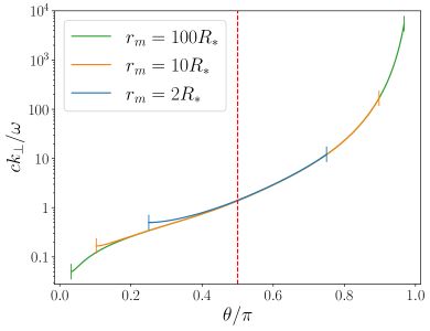
Figure 1: The evolution of $k_{\perp}$ on field lines of different $r_{m}$. The vertical markers indicate the footpoints of the magnetospheric field line on the star. The red dashed vertical line shows the magnetic equator $\theta=\pi/2$.

The variation of $k_{\perp}$ along a given field line is shown in Figure 1. For extended field lines, $r_{m}\gg r_{*}$, $k_{\perp}$ can grow to very large values in the southern hemisphere. This is a combination of two effects. The cumulative path difference $\partial s/\partial\eta$ grows fastest near the equator, which leads to $k_{\perp}\sim\omega/c$. Then, due to the field line convergence in the southern hemisphere, the existing $k_{\perp}$ is increased by a factor of $1/h_{\eta}\sim(r_{m}/r_{*})^{3/2}$ when the wave reaches the southern footpoint. After $N$ consecutive bounces, the wave will accumulate a total $ck_{\perp}\propto N\omega/h_{\eta}$, consistent with the result of Bransgrove et al. (2020) (their equation (38) used the approximation $\nabla_{\perp}\sim r^{-1}\partial_{\theta}$, which is valid for $\theta$ away from the equatorial plane).

The evolution of $ck_{\perp}/\omega$ results in the Alfvén wavefront becoming increasingly oblique with respect to the background field $\boldsymbol{B}_{0}$. The angle $\psi$ between the wave vector $\boldsymbol{k}$ and $\boldsymbol{B}_{0}$ grows as $\tan\psi=k_{\perp}/k_{\parallel}=ck_{\perp}/\omega$. The dimensionless parameter $\kappa$ grows as:

$$\kappa=\frac{j_{A}}{en_{0}c}\sim\frac{\omega_{B}\omega\tan\psi}{\omega_{p}^{2}}\,\frac{B_{w}}{B_{0}},$$ (9)

where $\omega_{p}=\sqrt{4\pi e^{2}n_{0}/m_{e}}$ is the background plasma frequency, and $\omega_{B}=eB_{0}/m_{e}c$ is the gyro-frequency of electrons in the background magnetic field. Due to the ever growing $\tan\psi$, the effect of wave shearing can eventually lead to charge-starvation, $\kappa>1$, even for waves of modest amplitudes.

3 Plasma dynamics in the wave: two-fluid model

3.1 Problem Setup

As a first step toward understanding charge-starved Alfvén waves, we examine a simple two-fluid model of plasma motion in a plane wave propagating into a uniform background. The uniform approximation is reasonable for sufficiently short waves. We take the background to be a cold neutral $e^{\pm}$ plasma with density $n_{+}=n_{-}=n_{0}=\mathrm{const}$ immersed in a uniform magnetic field $\boldsymbol{B}_{0}$. A gradual change of $\kappa$ may then be treated as an adiabatic effect on the quasi-steady plane wave.

We are interested in the highly magnetized regime with $\sigma\equiv B_{0}^{2}/4\pi n_{0}m_{e}c^{2}\gg 1$, so that the propagation speed of the wave along $\boldsymbol{B}_{0}$ nearly equals $c$. The electromagnetic field of a steadily propagating wave is then only a function of $t-s/c$, where the $s$-coordinate runs along $\boldsymbol{B}_{0}$. Let the $x$-axis be along the wave vector $\boldsymbol{k}$, the wave magnetic field $\boldsymbol{B}$ depends on

$$\xi=t-\frac{s}{c}=t-\frac{x}{c\cos\psi}.$$ (10)

The propagation speed along $x$ is $V_{x}=c\cos\psi$. The wave electric field $\boldsymbol{E}$ is related to the magnetic field $\boldsymbol{B}$ by

$$\boldsymbol{E}(\xi)=\boldsymbol{B}(\xi)\times\frac{\boldsymbol{B}_{0}}{B_{0}}.$$ (11)

The wave fields $\boldsymbol{B}$ and $\boldsymbol{E}$ are both perpendicular to the background field. The electric current density in the wave is parallel to $\boldsymbol{B}_{0}$ and its value is

$$j_{A}(\xi)=\frac{\tan\psi}{4\pi}\frac{dB}{d\xi}.$$ (12)

The charge density in the wave, $\rho=\nabla\cdot\boldsymbol{E}/4\pi$ satisfies the relation

$$c\rho(\xi)=j_{A}(\xi).$$ (13)

The above description gives an exact MHD solution in the force-free limit $\sigma\rightarrow\infty$ with no charge starvation. It relies on the implicit assumption that there is always enough plasma to conduct the required electric current $j_{A}$. We will next examine the dynamics of the $e^{\pm}$ particles for any given background plasma density $n_{0}$, especially in the regime $\kappa>1$, when the assumption of copious plasma supply may not be valid.

The characteristic gyro-frequency $\omega_{B}$ in the neutron star magnetosphere is many orders of magnitude greater than $\omega$. Therefore, $e^{\pm}$ particles in the wave move with velocities $\boldsymbol{v}$ along the magnetic field lines, like beads on a wire. Only $E_{\parallel}$ is relevant for their dynamics. For small amplitude waves $B_{w}\ll B_{0}$, the field lines are bent only by a small angle, and $v_{\parallel}=\boldsymbol{v}\cdot\boldsymbol{B}_{0}/B_{0}+{\cal O}(B_{w}^{2}/B_{0}^{2})$. Therefore we approximate the particle motion as parallel to $\boldsymbol{B}_{0}$.

In order to conduct the required electric current, an $E_{\parallel}$ will be induced to accelerate the electrons and positrons in opposite directions, creating two plasma streams.

3.2 Two-fluid Model

We first examine a simple model assuming that the $e^{\pm}$ streams remain cold, neglecting any possible instabilities that may arise. This “two-fluid” model captures some basic features of the plasma dynamics in the wave. The parallel electric field regulating the velocities of the $e^{\pm}$ streams is non-dissipative in the two-fluid model, as the particles will come to rest behind the wave.

The two cold fluids are described by their densities $n_{\pm}$ and velocities $v_{\pm}$. Both are functions of $\xi$ in a steadily propagating wave. Their values in the background plasma, $n_{\pm}=n_{0}$ and $v_{\pm}=0$, give the boundary conditions ahead of the wave for the profiles $n_{\pm}(\xi)$ and $v_{\pm}(\xi)$. The density and velocity of each stream satisfies the continuity equation $\partial_{t}n_{\pm}+\partial_{x}(n_{\pm}v_{\pm,x})=0$, where $v_{\pm,x}=v_{\pm}\cos\psi$. This gives

$$\frac{dn_{\pm}}{d\xi}-\frac{d}{d\xi}(n_{\pm}\beta_{\pm})=0,$$ (14)

where $\beta_{\pm}=v_{\pm}/c$. One then finds $(1-\beta_{\pm})dn_{\pm}=n_{\pm}d\beta_{\pm}$ and

$$n_{\pm}(\xi)=\frac{n_{0}}{1-\beta_{\pm}(\xi)},$$ (15)

where we used the boundary condition ahead of the wave: $n_{\pm}=n_{0}$ when $v_{\pm}=0$. In the two-fluid picture, the continuity equation automatically implies the relation $j=\rho c$, where $j=e(n_{+}v_{+}-n_{-}v_{-})$ and $\rho=e(n_{+}-n_{-})$.

The fluid velocities are related to $\kappa=j_{A}/en_{0}c$ by

$$\frac{1}{1-\beta_{+}}-\frac{1}{1-\beta_{-}}=\kappa(\xi).$$ (16)

In a successfully propagating Alfvén wave, the plasma motion must sustain $j=j_{\rm A}$ given in Equation (12), which determines $\kappa(\xi)$. Our goal is to find $\beta_{\pm}(\xi)$ under a given $\kappa(\xi)$, and then check what happens in the charge starvation regime of $\kappa>1$.

Particles are governed by the equation of motion $dp_{\pm}/dt=\pm eE_{\parallel}$, where $p_{\pm}=\gamma_{\pm}m_{e}v_{\pm}$, $\gamma_{\pm}=(1-\beta_{\pm}^{2})^{-1/2}$, and $d/dt=\partial_{t}+v_{\pm}d/ds=(1-\beta_{\pm})d/d\xi$. This equation gives

$$\frac{dq_{\pm}}{d\xi}=\pm\frac{eE_{\parallel}}{m_{e}c},\qquad q_{\pm}\equiv\gamma_{\pm}(1-\beta_{\pm}).$$ (17)

It implies $d(q_{+}+q_{-})/d\xi=0$. Then using the boundary condition $q_{+}=q_{-}=1$ ahead of the wave, we obtain

$$q_{+}+q_{-}=2.$$ (18)

Rewriting Equation (16) in terms of $q_{\pm}$,

$$\frac{1}{q_{+}^{2}}-\frac{1}{q_{-}^{2}}=2\kappa(\xi),$$ (19)

we obtain two equations for $q_{\pm}$, which can be easily solved for any given $\kappa(\xi)$. Once $q_{\pm}(\xi)$ are found, we also obtain $eE_{\parallel}=m_{e}c\,dq_{+}/d\xi$.

A well-behaved solution to the Equations (18) and (19) exists for both $|\kappa|<1$ and $|\kappa|>1$. In particular, consider $\kappa\gg 1$, the strongly “charge-starved” regime with $j>0$. Then the solution is $q_{+}^{-2}\approx 2\kappa\gg q_{-}^{-2}\approx 1/4$. Using the relation $q^{-1}=\gamma(1+\beta)$, we find

$$\gamma_{+}\approx\left(\frac{\kappa}{2}\right)^{1/2},\quad\gamma_{-}\approx\frac{5}{4}\qquad(\kappa\gg 1).$$ (20)

Figure 2 shows the solution for $p_{\pm}(\xi)$, and the corresponding $E_{\parallel}(\xi)$, for a plane wave with the following profile

$$\frac{B}{B_{w}}=\begin{cases}\displaystyle\frac{8}{3\sqrt{3}}\sin\left(2\pi\frac{\xi}{\lambda}\right)\sin^{2}\left(\pi\frac{\xi}{\lambda}\right),&\quad 0<\xi<\lambda\\ \displaystyle 0,&\quad\mathrm{otherwise}\end{cases}$$ (21)

This profile describes an isolated sine pulse, with the additional factor of $\sin^{2}(\pi\xi/\lambda)$ introduced to make the derivative $dB/d\xi$ smoothly vanish at the boundaries of the pulse $\xi=0,\lambda$. In our example, $\kappa(\xi)$ reaches the maximum $\kappa_{w}=10$ at $\xi=0.5\lambda$.

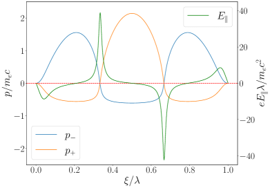
Figure 2: The momentum profile $p_{\pm}(\xi)$ of the electron (blue) and positron (orange) streams in the two-fluid model, for the wave profile given in equation (21). The corresponding $E_{\parallel}(\xi)$ is shown by the green curve. The maximum $\kappa$ in this example is $10$, reached at the center of the wave profile.

The wave achieves the required $j$ and $\rho$ by inducing $E_{\parallel}$ that sweeps the $e^{\pm}$ particles along $\boldsymbol{B}_{0}$. This sweeping compresses the two fluids by the factors of $(1-\beta_{\pm})^{-1}$ (Equation 15). In the regime of $\kappa\gg 1$ the compression factor is large for $e^{+}$, $(1-\beta_{+})^{-1}\approx 2\gamma_{+}^{2}$. Developing $\gamma_{\pm}\approx(\kappa/2)^{1/2}$ is sufficient to enhance the local density of $e^{+}$ by the factor of $\kappa$ and thus achieve $\rho$ and $j$ required by the wave. Particles move through the wave with the relative speed $c-v\approx c/2\gamma^{2}$ when $\gamma\gg 1$; therefore it takes time $t\sim\kappa\lambda/c$ for the plasma to cross the wave.

It is convenient to define

$$n_{w}=\frac{j_{\rm A}}{ec}.$$ (22)

In the charge-starved regime $\kappa\gg 1$, the wave carries the density $n\approx n_{w}$, and the electromagnetic energy available per particle is described by

$$\sigma_{w}=\frac{B_{w}^{2}}{4\pi n_{w}m_{e}c^{2}}.$$ (23)

The wave propagation is weakly affected by charge-starvation as long as $\gamma_{+}\approx(\kappa/2)^{1/2}\ll\sigma_{w}$. Otherwise the plasma kinetic energy will become comparable to the field energy, leading to significant deviations of $\boldsymbol{E}(\xi)$ and $\boldsymbol{B}(\xi)$ from the force-free solution.

In neutron star magnetospheres, the plasma frequency $\omega_{p}$ is much higher than the frequencies of Alfvén waves launched by crustal motion. This implies that the two-fluid model is deficient, because the cold two-stream configuration is unstable on the short plasma timescale $\sim\omega_{p}^{-1}$. In particular, consider the vicinity of a maximum of $p_{\pm}$ in Figure 2, where the two-fluid model gives $E_{\parallel}\approx 0$. Since the parameters of the $e^{\pm}$ streams are varying slowly compared to the plasma scale, $\omega\ll\omega_{p}$, one can use the standard linear instability analysis (e.g. Melrose, 1986) to find that the most unstable mode is near $k\sim\omega_{p}/c$ with growth rate $\Gamma\sim\omega_{p}$. The instability will heat the plasma streams and mix them in the phase space. It is difficult to predict analytically the consequences of the nonlinear saturation of the instability. Therefore, we employ direct kinetic plasma simulations to find a self-consistent solution.

4 Numerical Simulations

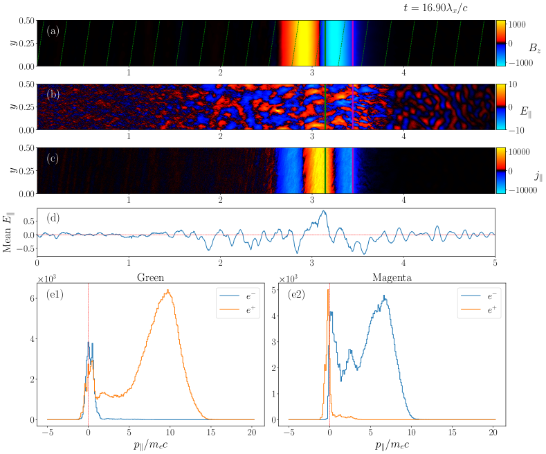
Figure 3: A snapshot of the simulation with $\kappa=12$. Panels from top to bottom are: (a) the wave magnetic field $B_{z}$ as color plot and $B_{0}$ as dashed green lines; (b) parallel electric field; (c) parallel current density; (d) $E_{\parallel}$ averaged over $y$; (e1) momentum distribution of $e^{\pm}$ in the green region depicted in panels (a)–(c); (e2) momentum distribution of $e^{\pm}$ in the magenta region in panels (a)–(c). $B$ and $E$ are measured in units of $m_{e}c^{2}/e\lambda_{x}$, while $j$ is measured in units of $m_{e}c^{3}/4\pi e\lambda_{x}^{2}$. These are the units used in the code.

4.1 Simulation Setup

We set up a series of Particle-in-Cell (PIC) simulations using our own GPU-based PIC code Aperture. We use a two-dimensional, elongated Cartesian box with periodic boundary conditions in the $y$ direction. An Alfvén wave is initialized at the left end of the box with the profile described by Equation (21), with magnitude $B_{w}$ and wave $\boldsymbol{B}$ pointing in the $z$ direction. The wave electric field is initialized using equation (11). The background magnetic field $\boldsymbol{B}_{0}$ is inclined with respect to the $x$-axis by an angle $\psi$. In our simulations, $\cos\psi=\hat{\boldsymbol{B}}_{0}\cdot\hat{\boldsymbol{x}}=0.15$. As the wave propagates along $\boldsymbol{B}_{0}$, it will move in the box along the $x$ direction. The effective length of propagation is much longer than the box length due to the inclination of the background field. A damping layer is placed at the end of the box $x=L_{x}$ to prevent the reflection of any plasma waves.

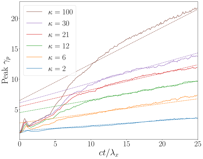
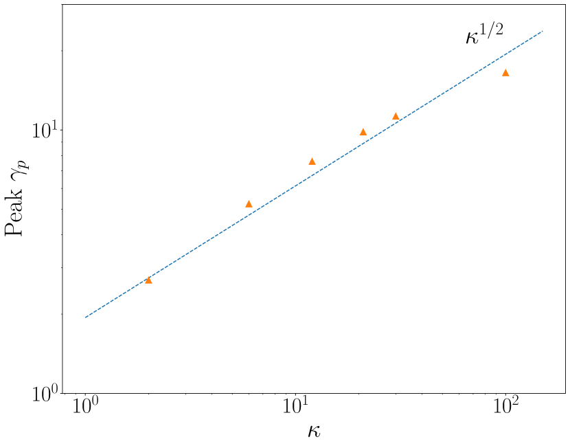
Figure 4: Particle Lorentz factor vs $\kappa$. Left panel: growth of peak Lorentz factor of the current conducting particles in the wave at different $\kappa$. Dashed lines have slopes $0.4\sqrt{\kappa}/\lambda$, and are acceleration models with constant $E_{\parallel}$. Right panel: orange triangles are peak Lorentz factors at $ct/\lambda_{x}=15$, while the blue dashed line indicates a simple power law $\gamma_{p}\propto\kappa^{1/2}$, which is the prediction of the two-fluid toy model.

We start with a small amplitude wave, with $B_{w}/B_{0}=0.1$. Inside the wave packet, we initialize a pair plasma that satisfies $\rho=j_{A}/c$ and $j=j_{A}$ with a small initial multiplicity, $n_{+}+n_{-}=3j_{A}/ec$. The space outside the wave packet is filled with a low density neutral plasma with $n_{+}=n_{-}=n_{0}$. We typically have 5–10 particles per cell corresponding to $n_{0}$. Depending on the value of $\kappa$ the number of particles per cell in the wave is often much larger. The characteristic plasma skin depth $c/\omega_{p}$ in the wave is set by $j_{A}/ec$, and is typically $\sim 1/200$ of the wavelength in the $x$ direction, $\lambda_{x}$. The box size is $L_{x}=5\lambda_{x}=10L_{y}$, and has a total resolution $5120\times 512$. This translates to $\sim 5$ cells per plasma skin depth. Outside the wave packet, where plasma density $n_{0}\ll j_{A}/ec$, the plasma skin depth is resolved with many more cells.

There are two dimensionless parameters, $\kappa$ and $\sigma_{w}$, that govern the physics in this problem. In the following discussion we refer to $\kappa$ as its maximum value at the center of the wave profile. In the simulations shown below we always keep $\sigma_{w}\sim 100$ so that $\sigma_{w}\gg\sqrt{\kappa}$. This is the realistic regime for Alfvén waves in a neutron star magnetosphere. The simulation results will verify that, in this limit, the amount of wave energy converted to particle kinetic energy is small, and the wave electromagnetic fields remain close to the initial force-free solution.

4.2 Waves in A Uniform Background

We performed a series of simulations where $\kappa$ is constant in the box, and increase $\kappa$ from 2 to 100 between the different runs. In these simulations, we observe that the cold two-stream instability rapidly develops and heats up the plasma streams. As a result of the nonlinear saturation of the instability, $E_{\parallel}$ breaks into Langmuir modes that are advected with the Alfvén wave. Figure 3 shows a snapshot of such a state in one of our PIC simulations with $\kappa=12$. The plasma momentum distribution in the wave can be generally described as a mildly relativistic, current conducting beam traveling into a neutral plasma at rest. This configuration is also subject to a warm version of the two-stream instability, exciting electrostatic wave modes that scatter the fast moving particles to lower velocities, creating a “bridge” between the two momentum peaks (see panel (e) in Figure 3). These slower particles tend to fall behind the current-carrying beam, reducing $j$. As a result, the plasma responds by inducing a small $E_{\parallel}$ on average which keeps accelerating the particles traveling in the wave. Effectively, this creates an anomalous resistivity that continually dissipates the Alfvén wave energy. A small fraction of this dissipated energy is converted into plasma waves launched into the upstream, but most of the energy goes into gradual acceleration of the relativistic beam.

Figure 4 shows this gradual and continual acceleration of the current conducting particles, as well as the scaling of their Lorentz factor with $\kappa$. At any given time, the peak Lorentz factor scales as $\sqrt{\kappa}$, which agrees with the two-fluid toy model. The acceleration in all cases seems to be consistent with an average $E_{\parallel}\approx 0.4\sqrt{\kappa}m_{e}c^{2}/e\lambda$, where $\lambda$ is the full wavelength of the Alfvén wave.

This mean electric field $E_{\parallel}$ is smaller than the (non-dissipative) spike of $E_{\parallel}$ that was needed in the two-fluid model to polarize the background plasma. The fractional dissipation rate of the wave energy density $U_{w}$ can be estimated as

$$\frac{\dot{U}_{w}}{U_{w}}\sim\frac{E_{\parallel}j_{A}}{B^{2}_{w}/8\pi}\sim\frac{\sqrt{\kappa}c}{\sigma_{w}\lambda}.$$ (24)

Thus, a fraction $\sqrt{\kappa}/\sigma_{w}$ of the initial electromagnetic energy in the Alfvén wave is dissipated in one crossing time of the wave $\lambda/c$.

This slow acceleration should saturate if beam reaches the group speed of the wave,

$$v_{A}=\sqrt{\frac{\sigma}{1+\sigma}},\quad\gamma_{A}=\sqrt{1+\sigma},$$ (25)

where $\sigma=B_{0}^{2}/4\pi n_{w}m_{e}c^{2}$ is the magnetization parameter, and $n_{w}$ is the plasma density in the wave, which can significantly exceed the background $n_{0}$ in the regime of $\kappa\gg 1$. The acceleration of the plasma beam carried by the wave should saturate when the beam Lorentz factor reaches $\gamma\sim\sqrt{\sigma}$, and further dissipation will likely go into heating up the plasma beam. Note, however, that it can take a long time for the wave to reach this saturated regime, and it may not occur in a real neutron star magnetosphere.

The fractional dissipation rate (24) scales with $\kappa$ and $\sigma_{w}$, and it is independent of the Alfvén wave amplitude $B_{w}/B_{0}$. We performed a series of simulations with the same $B_{w}$ and different background magnetic field strengths $B_{0}$, such that $B_{w}/B_{0}$ ranges from 0.01 to 0.5. We find that in all cases, as long as $B_{w}$ and $\kappa$ remains constant and $\sigma_{w}\gg\sqrt{\kappa}$, the energy dissipation rates and particle acceleration histories are identical.

Using the volume of the emission region $V\sim\lambda\ell_{\perp}2\pi r\sin\theta$, one can estimate the maximum luminosity from this slow dissipation if the particle kinetic energy gain can be converted to emission at some wavelengths:

$$\begin{split}L_{\mathrm{diss}}&\sim E_{\parallel}j_{A}V\\ &\sim\frac{\sqrt{\kappa}c}{\lambda}\frac{k_{\perp}B_{w}m_{e}c^{2}}{8\pi e}\lambda\ell_{\perp}2\pi r\sin\theta\\ &\sim\sqrt{\kappa}B_{w}r^{3/2}\frac{\pi m_{e}c^{3}}{2e}.\end{split}$$ (26)

Since $B_{w}=B_{w}^{\star}(r/r_{*})^{-3/2}$, the dissipation power is essentially only dependent on $\kappa$ and the initial Alfvén wave amplitude emitted by the star, $B_{w}^{\star}$.

4.3 Wave Propagation through a Density Jump

The numerical results described in Section 4.2 apply to a wave undergoing slow shearing, or propagating in a background plasma with a slowly varying density. We now investigate the opposite regime where $\kappa$ increases suddenly, on a length scale that is comparable or shorter than the Alfvén wavelength. In particular, we wish to check whether there is any dramatic transient behavior in the extreme limit when the Alfvén wave propagates across a sharp boundary where $\kappa$ transitions from $<1$ to $\gg 1$.

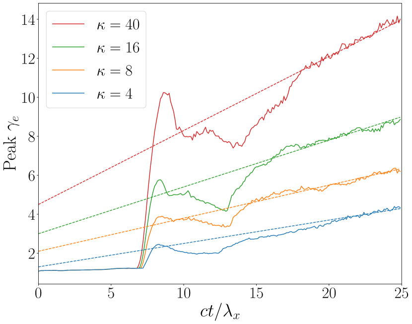
Figure 5: Evolution of maximum electron Lorentz factor vs $\kappa$ when there is a density jump. Dashed lines have slopes $0.4\sqrt{\kappa}/\lambda$, and are acceleration models with constant $E_{\parallel}$. After the transient when the wave goes across the density jump, particle acceleration proceeds in a similar fashion as Figure 4.

We use the same simulation setup as described in Section 4.2, with the exception that $n_{0}$ drops sharply at $x=0.4L_{x}$. We have carried out a series of simulations where $\kappa=0.8$ for $x<0.4L_{x}$ and $\kappa$ for $x>0.4L_{x}$ is a constant value above unity. In our simulations, the value of $\kappa$ after the jump ranges from 4 to 40. Figure 5 shows the evolution of peak electron Lorentz factors for these runs before and after the density jump.

We find that during its encounter with the density jump, the Alfvén wave induces a coherent $E_{\parallel}\propto\sqrt{\kappa}/\lambda_{x}$ to quickly accelerate charges of the right sign to $\gamma\sim\sqrt{\kappa}$. The parallel electric field separates the charges and sweeps the right amount of $e^{\pm}$ with the wave to conduct the required current. The most significant acceleration happens near the leading edge of the wave, which is negatively charged in our wave profile (see panel (c) of Figure 3). The encounter phase with the high $E_{\parallel}$ has a short duration, and the total dissipated energy during the simulation remains to be dominated by the later phase, when the wave continues to propagate through the low-density background. At this late phase, the wave behavior is similar to that found in Section 4.2 with $\kappa=\mathrm{const}$.

5 Discussion

We have studied the propagation of Alfvén waves in different plasma densities, in particular when the background plasma density is insufficient to support the required current $j_{A}$. In this “charge-starved” regime, the Alfvén wave manages to still provide the required current and charge densities by sweeping the charges of the right sign with it. The wave becomes charge-separated rather than truly charge-starved, and the charge carriers move at near the speed of light. In the highly magnetized regime relevant to neutron star magnetospheres, only a small amount of the Alfvén wave energy needs to be converted to particle kinetic energy to sustain this configuration.

The particle acceleration process is slow and smooth, with only a small induced $E_{\parallel}$ on average. There are two contributions to the acceleration of particles. As the “charge-starvedness” parameter $\kappa$ increases, the characteristic Lorentz factor for the charge carriers in the wave increases as $\sqrt{\kappa}$. At the same time, when $\kappa\gtrsim 1$, the current carrying particles are also accelerated by a nonzero dissipative $E_{\parallel}\propto\sqrt{\kappa}/\lambda$, even when $\kappa$ is constant.

We find that the transition to the regime of $\kappa>1$ leads to the dissipation rate given by the simple estimate (26). Below we use the parameters of the X-ray bursts from the galactic magnetar SGR 1935+2154 as an illustrative example. The energy budget of the X-ray burst is consistent with an Alfvén wave of amplitude $B_{w}^{\star}\sim 10^{-3}B_{p}\sim 10^{11}\,\mathrm{G}$ (Yuan et al., 2020). Assuming a large $\kappa\sim 100$, we can then estimate the maximum luminosity generated by the wave entering charge starvation as

$$L_{\mathrm{diss}}\approx 8\times 10^{34}\left(\frac{\kappa}{100}\right)^{1/2}\left(\frac{B_{w}^{\star}}{10^{11}\,\mathrm{G}}\right)\,\mathrm{erg/s}.$$ (27)

It is 5 orders of magnitude lower than the X-ray burst luminosity. It is also much lower than the luminosity of the FRB produced by SGR 1935+2154. The FRB energy output was $\sim 3\times 10^{34}\,\mathrm{erg}$, lasting about $1\,\mathrm{ms}$, which implies an isotropic equivalent luminosity of $\sim 3\times 10^{37}\,\mathrm{erg/s}$ (The CHIME/FRB Collaboration et al., 2020). Even assuming a huge $\kappa$ and a very high radiation efficiency of order unity, the luminosity (27) is insufficient to power the observed FRB. Furthermore, our simulations do not show strong bunching of $e^{\pm}$ in the saturated plasma oscillations in the Alfvén wave, and therefore we do not expect efficient coherent emission. Even if the plasma did form bunches, the particles do not gain enough energy or sufficiently high Lorentz factors for coherent emission in the radio band. Therefore, we conclude that it is unlikely that FRBs are produced through the charge-starvation mechanism alone.

Our results also imply that an Alfvén wave entering charge starvation does not need to spawn new $e^{\pm}$ pairs to propagate. Acceleration of particles to pair-producing energies likely requires additional mechanisms, such as wave collisions and nonlinear cascades (e.g. Thompson & Blaes, 1998; Li et al., 2019). For instance, these processes may be essential for the quake-excited Alfvén waves during the glitch chocking of the Vela pulsar radio emission.

In the vicinity of magnetars, resonant inverse-Compton scattering of the thermal X-ray photons flowing from the star can exert an efficient drag force on the plasma even when particle Lorentz factors are on the order of $\sim 10$, depending on the position in the magnetosphere (Beloborodov, 2013; Thompson & Kostenko, 2020). This can create a significant additional channel for dissipation of the Alfvén wave, which can potentially convert most of the energy gained by the particles into hard X-ray emission. The resulting X-ray luminosity may well be in the observable range. The inverse Compton scattering may also induce pair production which increases the background plasma density and thus reduces $\kappa$. These effects will be studied in a future work.

We thank Dmitri Uzdensky and Jens Mahlmann for helpful discussions. A.C. is supported by NSF grants AST-1806084 and AST-1903335. Y.Y. is supported by a Flatiron Research Fellowship at the Flatiron Institute, Simons Foundation. A.M.B. is supported by NASA grant NNX 17AK37G, NSF grant AST 2009453, Simons Foundation grant #446228, and the Humboldt Foundation. Research at Perimeter Institute is supported in part by the Government of Canada through the Department of Innovation, Science and Economic Development Canada and by the Province of Ontario through the Ministry of Colleges and Universities.

References

- Beloborodov (2013) Beloborodov, A. M. 2013, ApJ, 777, 114, doi: 10.1088/0004-637X/777/2/114
- Blaes et al. (1989) Blaes, O., Blandford, R., Goldreich, P., & Madau, P. 1989, ApJ, 343, 839, doi: 10.1086/167754
- Bochenek et al. (2020) Bochenek, C. D., Ravi, V., Belov, K. V., et al. 2020, arXiv e-prints, arXiv:2005.10828. https://arxiv.org/abs/2005.10828
- Bransgrove et al. (2020) Bransgrove, A., Beloborodov, A. M., & Levin, Y. 2020, A Quake Quenching the Vela Pulsar, doi: 10.3847/1538-4357/ab93b7
- Duncan & Thompson (1992) Duncan, R. C., & Thompson, C. 1992, ApJ, 392, L9, doi: 10.1086/186413
- Goldreich & Julian (1969) Goldreich, P., & Julian, W. H. 1969, ApJ, 157, 869, doi: 10.1086/150119
- Kumar & Bošnjak (2020) Kumar, P., & Bošnjak, Ž. 2020, MNRAS, 494, 2385, doi: 10.1093/mnras/staa774
- Kumar et al. (2017) Kumar, P., Lu, W., & Bhattacharya, M. 2017, MNRAS, 468, 2726, doi: 10.1093/mnras/stx665
- Li et al. (2019) Li, X., Zrake, J., & Beloborodov, A. M. 2019, ApJ, 881, 13, doi: 10.3847/1538-4357/ab2a03
- Lu et al. (2020) Lu, W., Kumar, P., & Zhang, B. 2020, arXiv e-prints, arXiv:2005.06736. https://arxiv.org/abs/2005.06736
- Melrose (1986) Melrose, D. B. 1986, Instabilities in Space and Laboratory Plasmas
- Mereghetti et al. (2020) Mereghetti, S., Savchenko, V., Ferrigno, C., et al. 2020, arXiv e-prints, arXiv:2005.06335. https://arxiv.org/abs/2005.06335
- Palfreyman et al. (2018) Palfreyman, J., Dickey, J. M., Hotan, A., Ellingsen, S., & van Straten, W. 2018, Nature, 556, 219, doi: 10.1038/s41586-018-0001-x
- Ruderman (1976) Ruderman, M. 1976, ApJ, 203, 213, doi: 10.1086/154069
- Swisdak (2006) Swisdak, M. 2006, arXiv e-prints, physics/0606044. https://arxiv.org/abs/physics/0606044
- The CHIME/FRB Collaboration et al. (2020) The CHIME/FRB Collaboration, :, Andersen, B. C., et al. 2020, arXiv e-prints, arXiv:2005.10324. https://arxiv.org/abs/2005.10324
- Thompson & Blaes (1998) Thompson, C., & Blaes, O. 1998, Phys. Rev. D, 57, 3219, doi: 10.1103/PhysRevD.57.3219
- Thompson & Kostenko (2020) Thompson, C., & Kostenko, A. 2020, arXiv e-prints, arXiv:2008.08659. https://arxiv.org/abs/2008.08659
- Yuan et al. (2020) Yuan, Y., Beloborodov, A. M., Chen, A. Y., & Levin, Y. 2020, ApJ, 900, L21, doi: 10.3847/2041-8213/abafa8