Gouy phase of type-I SPDC-generated biphotons

Abstract

We consider a double Gaussian approximation to describe the wavefunction of twin photons (also called a biphoton) created in a nonlinear crystal via a type-I spontaneous parametric downconversion (SPDC) process. We find that the wavefunction develops a Gouy phase while it propagates, being dependent of the two-photon correlation through the Rayleigh length. We evaluate the covariance matrix and show that the logarithmic negativity, useful in quantifying entanglement in Gaussian states, although Rayleigh-dependent, does not depend on the propagation distance. In addition, we show that the two-photon entanglement can be connected to the biphoton Gouy phase as these quantities are Rayleigh-length-related. Then, we focus the double Gaussian biphoton wavefunction using a thin lens and calculate a Gouy phase that is in reasonable agreement with the experimental data of D. Kawase et al. published in Ref. [1].

1 Introduction

Since its first detection in 1890 by L. G. Gouy [2, 3], the Gouy phase and its properties have been extensively studied [4-11]. This phase appears whenever a wave is constrained transversally to its propagation, which includes diffraction through slits and focus by lenses. The acquired phase depends on the type of transversal confinement and on the geometry of the waves. For example: line-focusing a cylindrical wave propagating from $-\infty$ to $+\infty$ yields a Gouy phase of $\pi/2$, while point-focusing a spherical wave in the same interval yields a Gouy phase of $\pi$ [6]; Gaussian matter wave packets diffracting through small apertures pick up a Gouy phase of $\pi/4$ [12].

The Gouy phase has been detected in various scenarios, including acoustic and water waves [17, 18, 19], surface plasmon-polaritons with non Gaussian spatial properties [15], focused cylindrical phonon-polariton wave packets in LiTaO₃ crystals, and more recently for electron waves [17, 18, 19]. Its presence in many systems justifies potential applications. To name a few, the Gouy phase is fundamental in evaluating the resonant frequencies in laser cavities [20], in phase-matching in strong-field and high-order harmonic generation [21], and in describing the spatial profile of laser pulses with high repetition rate [22]. In addition, an extra Gouy phase appears in optical and matter waves depending on the orbital angular momentum’s magnitude [23, 18]. In a recent work, it was found that the Gouy phase may cause nonlocal effects that modify the symmetries of self-organization in atomic systems [24]. This phase may also be useful in communication and optical tweezers using structured light [25].

The Gouy phase is also relevant in coherent matter waves, as shown for the first time in [12, 26, 27, 28]. Following that, experiments were performed in a number of systems, including Bose-Einstein condensates [17], electron vortex beams [18] and astigmatic electron waves [19]. Gouy phases in matter waves also display potential applications, namely: they can be used in mode converters in quantum information systems [26], in the generation of singular electron optics [19] and in the study of non-classical (exotic or looped) paths in interference experiments [29]. In this work, we are interested in the Gouy phase of entangled photon pairs generated in a type-I SPDC process.

An SPDC process generates a pair of entangled photons respecting energy-momentum conservation. These processes happen with extremely low probability – around $10^{-7}$ [30]. Because the first experiments involved non degenerate emerging photon beams, one with frequency in the IR and the other in the visible range, they were named idler and signal, respectively [31]. The emerging photons in these processes are highly correlated in energy, momentum, polarization and angular momentum [32]. They emerge after a pump beam, with frequency $\omega_{p}$, goes through a nonlinear crystal, generating (in those very rare cases) two lower energy photons, the idler and signal, with frequencies $\omega_{i}$ and $\omega_{s}$. The type of SPDC depends on the polarization of the emerging photons with respect to the incoming pump beam. For example, in a type-I SPDC, the signal and idler photons display parallel polarizations, both orthogonal to the pump beam’s, and form a cone aligned to the pump beam’s direction. In a type-II SPDC the signal and idler photons have orthogonal polarizations and emerge in 2 different cones. The spatial distribution of the emerging beams is a consequence of energy-momentum conservation: $\omega_{p}=\omega_{i}+\omega_{s}$ and $\vec{k}_{p}=\vec{k}_{i}+\vec{k}_{s}$. This also causes the high degree of energy-momentum correlations between the emerging beams. For a more details, please consult Ref. [33] and the references therein. In fact, it is possible to control the correlations between different degrees of freedom in the generated pairs [34]. In this work, we will consider twin photons with wavelength $702.2\,$nm, typically used in interferometry experiments, such as in Refs. [35, 36].

Regarding the entanglement, the Schmidt number plays an important role. The propagation dynamics of spatially entangled biphotons was explored via the Schmidt number in Ref. [37]. Like the logarithmic negativity, the Schmidt number is propagation-distance-independent and the entanglement migrates between amplitude and transverse phase. In this work we will explore the two-photon entanglement by means of the longitudinal Gouy phase of the double Gaussian approximation for the biphoton wavefunction. We calculate the Gouy phase for this approximated biphoton wavefunction and show that it is related with the photon correlation generated in the nonlinear crystal in a type-I SPDC process. Even though the photon entanglement is time-independent, whereas the Gouy phase is time dependent, these quantities become related by the Rayleigh length. More interestingly we show that the approximated biphoton Gouy phase fits well the experimental data published in Ref. [1].

The article is organized as follows: in section II we propagate the double Gaussian biphoton wavefunction and obtain the corresponding Gouy phase. In section III we evaluate the covariance matrix and the logarithmic negativity and show that the two-photon entanglement is longitudinal-distance-independent. We observe that the entanglement measured by the logarithmic negativity and the Gouy phase are related by the Rayleigh length. In section IV we focus the double Gaussian biphoton wavefunction and use the corresponding Gouy phase to analyze the existing experimental data. In section V we draw our concluding remarks.

2 Propagation of biphoton wavefunction and Gouy phase

In this section we propagate a double Gaussian biphoton wavefunction using free-particle propagators. Then, we obtain a Gaussian solution expressed in terms of real terms and phases. One of the phases is the Gouy phase, which is transverse-position-independent and is a function of the longitudinal distance of propagation, the beam pump parameters, and the twin photon correlation. We consider as the initial biphoton wavefunction the following entangled state [38, 39, 40]

$$\Psi(x_{1},x_{2})=\frac{1}{\sqrt{\pi\sigma\Omega}}e^{\frac{-(x_{1}-x_{2})^{2}}{4\sigma^{2}}}e^{\frac{-(x_{1}+x_{2})^{2}}{4\Omega^{2}}},$$ (1)

which is the generalized EPR state for the momentum-entangled particles. Here, $\Omega$ and $\sigma$ quantify the position and momentum uncertainties of the packet, i.e., $\Delta x_{1}=\Delta x_{2}=\sqrt{\Omega^{2}+\sigma^{2}}$ and $\Delta p_{x1}=\Delta p_{x2}=(\hbar/4)\sqrt{(1/\Omega^{2})+(1/\sigma^{2})}$. This approximated biphoton state is correlated only if $\Omega\neq\sigma$ and $\Omega=\sigma$ corresponds to a non entangled state which factors as a product of two Gaussians [40].

We will work with relative coordinates $r=(x_{1}+x_{2})/2$ and $q=(x_{1}-x_{2})/2$ since these are convenient for calculations. Thus, the initial wavefunction that represents the entangled state can be rewritten as

$$\Psi(r,q)=\frac{1}{\sqrt{\pi\sigma\Omega}}e^{-\frac{q^{2}}{\sigma^{2}}}e^{-\frac{r^{2}}{\Omega^{2}}}.$$ (2)

The state describing the biphoton free propagation can be written as

$$\Psi(r,q,t)=\int_{r^{\prime},q^{\prime}}K_{r}(r,t;r^{\prime},0)K_{q}(q,t;q^{\prime},0)\psi(r^{\prime},q^{\prime}),$$ (3)

where the propagation kernels of a longitudinal distance $z=ct$ for the two photons are given by

$$\begin{split}K_{r}(r,r^{\prime},z)=\sqrt{\frac{1}{i\lambda z}}\exp{\bigg{[}-\frac{2\pi(r-r^{\prime})^{2}}{i\lambda z}\bigg{]}},\\ K_{q}(q,q^{\prime},z)=\sqrt{\frac{1}{i\lambda z}}\exp{\bigg{[}-\frac{2\pi(q-q^{\prime})^{2}}{i\lambda z}\bigg{]}}.\end{split}$$ (4)

The state after a general distance $z$ can be evaluated as

$$\Psi(r,q,z)=\frac{1}{\sqrt{4\pi w_{+}(z)w_{-}(z)}}\exp\bigg{\{}-\bigg{[}\frac{r^{2}}{w_{+}^{2}(z)}+\frac{q^{2}}{w_{-}^{2}(z)}\bigg{]}\bigg{\}}\\ \times\exp\bigg{\{}-i\bigg{[}-\frac{k_{0}}{r_{+}}r^{2}-\frac{k_{0}}{r_{-}}q^{2}+\zeta(z)\bigg{]}\bigg{\}},$$ (5)

where,

$$w_{\pm}^{2}(z)=\Omega^{2}\bigg{[}1+\bigg{(}\frac{z}{z_{0\pm}}\bigg{)}^{2}\bigg{]},\hskip 14.22636ptr_{\pm}(z)=z\bigg{[}1+\bigg{(}\frac{z_{0\pm}}{z}\bigg{)}^{2}\bigg{]},$$ (6)

$$z_{0+}=k_{0}\Omega^{2},\hskip 5.69046ptz_{0-}=k_{0}\sigma^{2}\hskip 5.69046pt\text{and}\hskip 5.69046ptk_{0}=2\pi/\lambda.$$ (7)

Now, considering the analogy with the classical Gaussian laser beam we can identify the biphoton wavefunction terms as: $w_{\pm}(z)$ is the beam width, $r_{\pm}(z)$ the radius of curvature of the wave fronts and $z_{0\pm}$ the corresponding Rayleigh lengths. The function $\zeta(z)$ is the biphoton Gouy phase that, after some algebraic manipulations, is written as

$$\zeta(z) = \frac{\zeta_{+}(z)}{2}+\frac{\zeta_{-}(z)}{2}$$ (8)

$$= \frac{1}{2}\arctan\bigg{[}z\bigg{(}\frac{z_{0+}+z_{0-}}{z_{0+}z_{0-}-z^{2}}\bigg{)}\bigg{]},$$

where $\zeta_{+}(z)=\arctan(z/z_{0+})$ and $\zeta_{-}(z)=\arctan(z/z_{0-})$. We can see that this phase is propagation-distance-dependent. It carries the properties of the laser pump beam and the nonlinear crystal through the parameter $\sigma=\sqrt{\frac{L_{p}\lambda_{p}}{6\pi}}$, where $\lambda_{p}$ is the laser pump wavelength and $L_{p}$ the crystal length. The two-photon correlation dependence can be measured through the parameter $\Omega$.

In Figure 1 we show the plot of the biphoton Gouy phase as a function of $z$. As in Ref. [42] we consider the following set of parameters: biphoton wavelength $\lambda=702\;\mathrm{nm}$, laser pump wavelength $\lambda_{p}=351.1\;\mathrm{nm}$ and the crystal length $L_{p}=7.0\;\mathrm{mm}$. This enables us to obtain $\sigma=\sqrt{\frac{L_{p}\lambda_{p}}{6\pi}}=11.4\;\mathrm{\mu m}$ and $z_{0-}=k_{0}\sigma^{2}=1.2\;\mathrm{mm}$. For the curve in blue we consider $\Omega=5\sigma$ and for the red curve we consider $\Omega=10\sigma$.

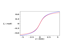
Figure 1: Biphoton Gouy phase as a function of $z$. The curve in blue corresponds to $\Omega=5\sigma$, and the curve in red corresponds to $\Omega=10\sigma$.

As we can observe, the maximum variation of the Gouy phase is $\pi/2$, characterizing one-dimensional free propagation from $z=-\infty$ to $z=+\infty$ with the beam waist located at the origin $z=0$ at the position of the crystal. Also, the smaller correlation produces a larger Gouy phase variation as we can see by comparing the curves in blue and red.

3 Entanglement and Gouy phase

Here we show how the two-photon entanglement is related with the parameters $\sigma$ and $\Omega$ and therefore with the Rayleigh length $z_{0\pm}$. In fact, the Rayleigh-length-dependence establishes a connection between the Gouy phase and two-photon entanglement. A good measure of entanglement for Gaussian states is the logarithmic negativity which is calculated through the covariance matrix. In the symplectic form the covariance matrix can be written as [38, 41]

$$M=\left[\begin{array}[]{cccc}g&0&c&0\\ 0&g&0&c^{\prime}\\ c&0&h&0\\ 0&c^{\prime}&0&h\end{array}\right]$$ (13)

which is related to

$G=\begin{bmatrix}\frac{\langle x_{1}^{2}\rangle}{L^{2}}&\frac{\langle x_{1}p_{1}+p_{1}x_{1}\rangle}{2\hbar}\\ \frac{\langle x_{1}p_{1}+p_{1}x_{1}\rangle}{2\hbar}&\frac{L^{2}\langle p_{1}^{2}\rangle}{\hbar^{2}}\end{bmatrix},H=\begin{bmatrix}\frac{\langle x_{2}^{2}\rangle}{L^{2}}&\frac{\langle x_{2}p_{2}+p_{2}x_{2}\rangle}{2\hbar}\\ \frac{\langle x_{2}p_{2}+p_{2}x_{2}\rangle}{2\hbar}&\frac{L^{2}\langle p_{2}^{2}\rangle}{\hbar^{2}}\end{bmatrix},\;C=\begin{bmatrix}\frac{\langle x_{1}x_{2}\rangle}{L^{2}}&\frac{\langle x_{1}p_{2}\rangle}{\hbar}\\ \frac{\langle x_{2}p_{1}\rangle}{\hbar}&\frac{L^{2}\langle p_{1}p_{2}\rangle}{\hbar^{2}}\end{bmatrix}$,

through the simple relations $\det G=g^{2}$, $\det H=h^{2}$ and $\det C=cc^{\prime}$. The constants $\hbar$ and $L$, which appear in the above matrices, are inserted to make the matrix $M$ dimensionless. For the next calculations $L$ can be disregarded (see [38] for further discussion on these constants). We obtain the quantities of $M$ in Eq. (13) as follows

$$\langle x_{1}^{2}\rangle=\langle x_{2}^{2}\rangle=(\sigma^{2}+\Omega^{2})\bigg{[}\bigg{(}\frac{z}{z_{0+}}\bigg{)}\bigg{(}\frac{z}{z_{0-}}\bigg{)}+1\bigg{]},$$ (14)

$$\langle x_{1}x_{2}\rangle=\langle x_{2}^{2}\rangle=(\sigma^{2}-\Omega^{2})\bigg{[}\bigg{(}\frac{z}{z_{0+}}\bigg{)}\bigg{(}\frac{z}{z_{0-}}\bigg{)}-1\bigg{]},$$ (15)

$$\langle p_{1}^{2}\rangle=\langle p_{2}^{2}\rangle=\frac{1}{4}\bigg{[}\frac{1}{\Omega^{2}}+\frac{1}{\sigma^{2}}\bigg{]},\hskip 14.22636pt\langle p_{1}p_{2}\rangle=\frac{1}{4}\bigg{[}\frac{1}{\Omega^{2}}-\frac{1}{\sigma^{2}}\bigg{]},$$ (16)

$$\langle x_{1}p_{2}\rangle=\langle x_{2}p_{1}\rangle=\frac{\pi\hbar}{2}\bigg{(}\frac{z}{z_{0+}}-\frac{z}{z_{0-}}\bigg{)},$$ (17)

and

$$\sigma_{xp} = \frac{\langle x_{1}p_{1}+p_{1}x_{1}\rangle}{2}=\frac{\langle x_{2}p_{2}+p_{2}x_{2}\rangle}{2}$$ (18)

$$= \frac{\pi\hbar}{2}\bigg{(}\frac{z}{z_{0+}}+\frac{z}{z_{0-}}\bigg{)}=\frac{\pi\hbar}{2}[\tan(\zeta_{+})+\tan(\zeta_{-})],$$

where $\zeta_{+}$ and $\zeta_{-}$ are parts of the biphoton Gouy phase from Eq. (8). A relation between these two quantities was obtained previously in the context of a single particle [26]. Here, we are showing that the biphoton Gouy phase is part of the logarithmic negativity (entanglement) through the position momentum covariance.

A strong necessary condition for an entanglement quantifier is that it has to be zero if the state is separable. The Peres-Horodecki criterion says that if a state is separable, the transpose partial matrix of the state has a non-negative spectrum. In that context, the Gaussian state is separable if and only if the minimum value of the symplectic spectrum of $M^{T_{2}}$ is greater than $1/2$ (the lowest value allowed by the uncertainty principle). Thus, a good measure of entanglement for all Gaussian states is the logarithmic negativity [38, 41]

$$E_{N}=max\{0,-\log(2\nu_{min})\},$$ (19)

where, $\nu_{min}$ is the lowest symplectic eigenvalue of $M^{T_{2}}$. The equation determining the symplectic eigenvalues is $\nu^{4}+(g^{2}+c^{2}-2cc^{\prime})\nu^{2}+det(M)=0$, with solutions $\pm i\nu_{\alpha}$, $\alpha=1,2$ where $\nu_{\alpha}$ is the symplectic spectrum. Therefore, $\nu_{1}=(\Omega/2\sigma)$ and $\nu_{2}=(\sigma/2\Omega)$. Due the uncertainty principle, $\nu_{min}<1/2$, so that the logarithmic negativity is given by

$$E_{N}=\begin{cases}\log\bigg{(}\sqrt{\frac{z_{0-}}{z_{0+}}}\bigg{)},&\mbox{if }z_{0+}\leq z_{0-}\mbox{;}\\ \\ \log\bigg{(}\sqrt{\frac{z_{0+}}{z_{0-}}}\bigg{)},&\mbox{otherwise.}\par\end{cases}$$ (20)

which is propagation-distance-independent. We observe in Eq. (20) that the entanglement measured by the logarithmic negativity can be modified by changing the Rayleigh length $z_{0+}$ since $z_{0-}$ is fixed by the laser pump properties. On the other hand, the double Gaussian biphoton wavefunction approximation shows no entanglement for $z_{0+}=z_{0-}$. In the analysis of Ref. [37], which uses the Schmidt number, the entanglement is Rayleigh-length-dependent and the case $z_{0+}=z_{0-}$ implies no entanglement within the spatial phase of entangled photon pairs. In [37] the authors compute the Schmidt number through their Eq. (6) for the double Gaussian wave function, which, using our wave function Eq. (5), can be written as

$$\begin{split}K_{dG}=&\bigg{(}\frac{w_{+}}{w_{-}}+\frac{w_{-}}{w_{+}}\bigg{)}^{2}+k_{0}^{2}w^{2}_{+}w^{2}_{-}\bigg{(}\frac{1}{r_{-}}-\frac{1}{r_{+}}\bigg{)}^{2}\\ =&\bigg{(}\sqrt{\frac{z_{0-}}{z_{0+}}}+\sqrt{\frac{z_{0+}}{z_{0-}}}\bigg{)}^{2},\end{split}$$ (21)

where $w_{\pm}$ and $r_{\pm}$ are given by Eq. (6). From Eqs. (20) and (21) we obtain $E_{N}=\log(\sqrt{K_{dG}})$ for $z_{0+}/z_{0-}\ll 1$ and $z_{0+}/z_{0-}\gg 1$. In Fig. 2 we compare the logarithmic negativity with the logarithm of the root square of the Schmidt number. In Fig. 2a we plot the logarithmic negativity and the logarithm of the root square of the Schmidt number as a function of $z_{0+}/z_{0-}\leq 1$ and in Fig. 2b we plot these quantities for $z_{0+}/z_{0-}\geq 1$. We observe an agreement of these quantities in the limits $z_{0+}/z_{0-}\ll 1$ and $z_{0+}/z_{0-}\gg 1$.

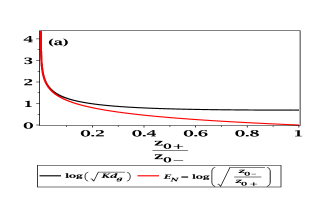
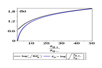
Figure 2: (a) Logarithmic negativity and the logarithm of the root square of the Schmidt number as a function of $z_{0+}/z_{0-}\leq 1$ and (b) the same quantities for $z_{0+}/z_{0-}\geq 1$. These quantities agree in the limits $z_{0+}/z_{0-}\ll 1$ and $z_{0+}/z_{0-}\gg 1$.

As the Gouy phase is a function of the Rayleigh length $z_{0+}$ and $z_{0-}$, one can measure this longitudinal phase as a function of the entanglement by changing the Rayleigh length $z_{0+}$ and fixing the parameters $z$ and $z_{0-}$ – see Eq. (8). To observe the behavior of logarithmic negativity and the Gouy phase as a function of $z_{0+}$, we plot these quantities in Fig. 3. We consider $z_{0-}=1.2\;\mathrm{mm}$ and the longitudinal position $z=20\;\mathrm{mm}$. In Fig. 3a we plot the logarithmic negativity and in Fig. 3b the Gouy phase as a function of $z_{0+}/z_{0-}\leq 1$. In Fig. 3c we plot the logarithmic negativity and in Fig. 3d the Gouy phase as a function of $z_{0+}/z_{0-}\geq 1$.

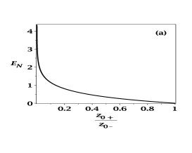
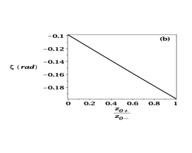
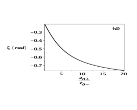
Figure 3: (a) Logarithmic negativity and (b) Biphoton Gouy phase for the Rayleigh range $z_{0+}/z_{0-}\leq 1$, (c) Logarithmic negativity and (d) Biphoton Gouy phase for the Rayleigh range $z_{0+}/z_{0-}\geq 1$, with $z_{0-}=1.2\;\mathrm{mm}$ and $z=20\;\mathrm{mm}$. The logarithmic negativity varies appreciably in both intervals whereas the Gouy phase variation is appreciable only for the interval $z_{0+}/z_{0-}\geq 1$ in which $z_{0+}$ tends to $z$.

We observe that the logarithmic negativity suffers a large variation for $z_{0+}/z_{0-}\leq 1$ whereas the Gouy phase does not vary significantly. However, for $z_{0+}/z_{0-}\geq 1$ the Gouy phase changes appreciably. It is known that the Gouy phase varies the most within the Rayleigh length. Therefore, the Gouy phase variation as a function of $z_{0+}$ in the position $z=20\;\mathrm{mm}$ will be small if $z\gg z_{0+}$ (which occurs for $z_{0+}\leq 1.2\;\mathrm{mm}$, i.e., for $z_{0+}/z_{0-}\leq 1$) and appreciable if $z_{0+}$ is of the order of $z$ (which occurs for $z_{0+}\geq 1.2\;\mathrm{mm}$, i.e., for $z_{0+}/z_{0-}\geq 1$). In the next section we will consider the two-dimensional propagation through a thin lens which enables us to adjust existing experimental data for the biphoton Gouy phase as a function of the shifted Rayleigh length.

4 Agreement with existing experimental data

In Ref. [1] the authors showed for the first time the relation between the Gouy phase and the quantum correlations of the twin photons generated by parametric down conversion. Then, they measured the coincidence count rates to experimentally obtain the Gouy phase as a function of the position of the beam waist. In this section we compare the biphoton Gouy phase with the experimental data obtained in Ref. [1]. In that experiment they considered as the pump a continuous wave (CW) argon-ion laser of wavelength $\lambda_{p}=351\;\mathrm{mm}$ and power $P=60\;\mathrm{mW}$, which was focused by a lens of focal distance $f=900\;\mathrm{mm}$ to the beam radius $w_{p}=178\;\mathrm{\mu m}$ in a BBO crystal of type I, which produces signal and idler photon beams with the same wavelength $\lambda=702\;\mathrm{nm}$. Also, they used lenses of focal distance $f=200\;\mathrm{mm}$ in the paths of the signal and idler beams. Therefore, by changing the position of the lens in the signal path (which corresponds to changing the position of its beam waist) while scanning with a two-dimensional hologram the idler path they were able to measure the coincidence counting rates in different positions of the signal beam waist. Then, by observing that the position of the maximum and minimum coincidences becomes rotated by a phase that includes the Gouy phase difference of the modes $LG_{00}$ and $LG_{0-1}$, they could relate the quantum correlation with the Gouy phase.

In order to analyze the experimental data of Ref. [1] we need to focus the biphoton wavefunction. Then, by considering a thin lens approximation, and focal length $f$, the focused biphoton wavefunction is given by

$$\begin{split}\Psi(r,q,z,z^{\prime})=&\int_{r^{\prime},q^{\prime}}K_{r}(r,r^{\prime};z+z^{\prime},z)K_{q}(q,q^{\prime};z+z^{\prime},z)f(r^{\prime},q^{\prime})\psi(r^{\prime},q^{\prime},z),\end{split}$$ (22)

where the propagators $K_{r}$ and $K_{q}$ are given by Eq. (4), the state $\psi(r^{\prime},q^{\prime},z)$ is written as Eq. (5) and the transmittance of a thin lens is given by [44, 45]

$$f(r^{\prime},q^{\prime})=\exp\bigg{[}-\frac{ik}{2f}(r^{\prime 2}+q^{\prime 2})\bigg{]}.$$ (23)

After some manipulations, we can write

$$\Psi(r,q,z,z^{\prime})=\sqrt{\frac{2}{\pi B_{+}B_{-}}}\exp\left(-\frac{r^{2}}{B^{2}}\right)\exp\left(-\frac{q^{2}}{B_{-}^{2}}\right)\exp\left[\frac{ik_{0}}{cR_{+}}r^{2}+\frac{ik_{0}}{cR_{-}}q^{2}-i\zeta(z,z^{\prime})\right],$$ (24)

where

$$B_{+}^{2}(z,z^{\prime})=\frac{\left(\frac{1}{w_{+}^{2}}\right)^{2}+k_{0}^{2}\left(\frac{1}{z^{\prime}}+\frac{1}{cr_{+}}-\frac{1}{2f}\right)^{2}}{\left(\frac{2\pi}{\lambda z^{\prime}}\right)^{2}\left(\frac{1}{w_{+}^{2}}\right)},$$ (25)

$$B_{-}^{2}(z,z^{\prime})=\frac{\left(\frac{1}{w_{-}^{2}}\right)^{2}+k_{0}^{2}\left(\frac{1}{z^{\prime}}+\frac{1}{cr_{-}}-\frac{1}{2f}\right)^{2}}{\left(\frac{2\pi}{\lambda z^{\prime}}\right)^{2}\left(\frac{1}{w_{-}^{2}}\right)},$$ (26)

$$R_{+}(z,z^{\prime})=\frac{\left(\frac{1}{w_{+}^{2}}\right)^{2}+k_{0}^{2}\left(\frac{1}{z^{\prime}}+\frac{1}{cr_{+}}-\frac{1}{2f}\right)^{2}}{\frac{c}{z^{\prime}w_{+}^{2}}\left(1+\frac{1}{\Omega^{2}}\left(\frac{z}{z^{\prime}}+\frac{z}{cr_{+}}\right)\right)-\frac{\pi}{\lambda f}},$$ (27)

$$R_{-}(z,z^{\prime})=\frac{\left(\frac{1}{w_{-}^{2}}\right)^{2}+k_{0}^{2}\left(\frac{1}{z^{\prime}}+\frac{1}{cr_{-}}-\frac{1}{2f}\right)^{2}}{\frac{c}{z^{\prime}w_{-}^{2}}\left(1+\frac{1}{\sigma^{2}}\left(\frac{z}{z^{\prime}}+\frac{z}{cr_{-}}\right)\right)-\frac{\pi}{\lambda f}},$$ (28)

and

$$\zeta(z,z^{\prime})=\frac{1}{2}\arctan\Bigg{\{}\frac{\big{(}\frac{z}{1-z^{\prime}/2f}+z^{\prime}\big{)}\big{(}\frac{1}{z_{0+}}+\frac{1}{z_{0-}}\big{)}}{1-\frac{1}{z_{0+}z_{0-}}\big{(}\frac{z}{1-z^{\prime}/2f}+z^{\prime}\big{)}^{2}}\Bigg{\}}.$$ (29)

Now, the parameters of the wavefunction are dependent on the focal distance $f$. By the analogy with the focused classical Gaussian beam, $B_{\pm}(z,z^{\prime})$ is the corresponding beam width, $R_{\pm}(z,z^{\prime})$ is the corresponding radius of curvature of the wavefronts and $\zeta(z,z^{\prime})$ is the corresponding Gouy phase. In the limit $f\rightarrow\infty$ we recover the parameters of the biphoton wavefunction in Eq. (5) for the propagation $z+z^{\prime}$. In Fig. 4 we plot the Gouy phase for the focused biphoton wavefunction Eq. (29) as a function of the position after the lens $z^{\prime}$. We consider the following parameters $z_{0+}=z_{0-}=1.2\;\mathrm{mm}$, $f=3.0\;\mathrm{mm}$ and $z=7.0\;\mathrm{mm}$. As we can observe the phase is null for $z^{\prime}=2f=6.0\;\mathrm{mm}$. Again the maximum Gouy phase variation is $\pi/2$ as we have considered the one-dimensional focalization.

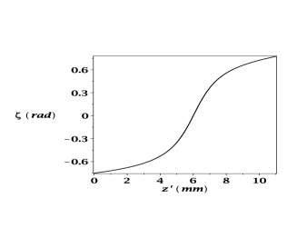
Figure 4: Gouy phase for the focused biphoton wavefunction Eq. (29) as a function of the position after the lens $z^{\prime}$.

Now, in order to use the biphoton Gouy phase to fit the experimental data of Ref. [1] we need to rewrite Eq. (29) to include the two-dimensional propagation through a thin lens which transforms it to

$$\zeta(z_{0+})=\zeta_{0}+\arctan\Bigg{\{}\frac{\big{(}\frac{z}{1-z^{\prime}/2f}+z^{\prime}\big{)}\big{(}\frac{1}{(z^{\prime}_{0+}-z_{f})}+\frac{1}{z_{0-}}\big{)}}{1-\frac{1}{(z^{\prime}_{0+}-z_{f})z_{0-}}\big{(}\frac{z}{1-z^{\prime}/2f}+z^{\prime}\big{)}^{2}}\Bigg{\}},$$ (30)

where $\zeta_{0}$ is a reference angle and $z_{f}$ an adjust parameter. In Fig. 5 we show the Gouy phase as a function of the Rayleigh range $z_{0+}$ shifted by an offset distance $z_{offset}$. The negative values appearing for $z_{0+}$ in the horizontal axis is a consequence of the shift by $z_{offset}$. The squares represent the experimental data from [1] and the solid line represents the fitting result by Eq. (30). As discussed before the two-photon entanglement is included in $z_{0+}$.

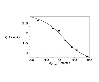
Figure 5: Gouy phase as a function of $z_{0+}$. The squares represents the experimental data from [1] and the solid line represents the fitting result Eq. (30).

In order to adjust the experimental data of Fig. 4 of Ref. [1] with Eq. (30) we used the Maple software which produces the following values of parameters: biphoton wavelength $\lambda=702\;\mathrm{nm}$, laser pump wavelength $\lambda_{p}=351.1\;\mathrm{nm}$ and the crystal length $L_{p}=7.0\;\mathrm{mm}$. This enables us to obtain $\sigma=\sqrt{\frac{L_{p}\lambda_{p}}{6\pi}}=11.4\;\mathrm{\mu m}$, $z_{0-}=k_{0}\sigma^{2}=1.2\;\mathrm{mm}$, $f=200\;\mathrm{mm}$, $z=500\;\mathrm{mm}$, $z^{\prime}=1465.3\;\mathrm{mm}$, $\zeta_{0}=1.68\;\mathrm{rad}$ and $z_{f}=7.15\;\mathrm{mm}$. Because of some effect of the experimental arrangement, such as that produced by the hologram, we need to include a parameter $z_{f}$ in Eq. (30) in order to adjust the experimental data. The reasonable agreement between theory and experimental data on the Gouy phase indicates the double Gaussian wavefunction is a valid approximate description of two correlated photons generated by type-I SPDC.

In Ref. [1] the Gouy phase was obtained by changing the position of the beam width $z_{0s}$. Here, we adjust the Gouy phase by changing the Rayleigh length $z_{0+}$ instead of $z_{0s}$. Now, we will show that these two quantities are related. The beam waist position $z^{+}_{0s}$ after a thin lens can be obtained from Eq. (25) and written as

$$z^{+}_{0s}=\frac{2ck_{0}^{2}w_{+}^{4}r_{+}(cr_{+}-2f)f}{k_{0}^{2}w_{+}^{4}(cr_{+}-2f)^{2}+4f^{2}c^{2}r_{+}^{2}},$$ (31)

where $w_{+}$ and $r_{+}$ are given by Eq. (6), $k_{0}$ is the wavenumber Eq. (7), $c$ is the speed of light and $f$ is the focal length. This quantity is $z_{0+}$-dependent trough the parameters $w_{+}$ and $r_{+}$. In order to observe the behavior of the beam waist position $z^{+}_{0s}$ as a function of the Rayleigh length $z_{0+}$, we plot it in Fig. 6. This plot shows that the beam waist position varies with the Rayleigh length. We consider the same parameters of Fig. 5.

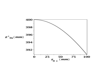
Figure 6: Beam waist position $z^{+}_{0s}$ as function of the Rayleigh range $z_{0+}$.

Therefore, this relation is the reason why one can also plot the experimental data of Ref. [1] as a function of the Rayleigh length. In addition, although the authors used a superposition of LG modes to observe the Gouy phase instead of a Gaussian mode, they observed that the superposition is converted into a Gaussian mode when the hologram is shifted and scanned to change the phase between LG modes. As we can see the expression found in Eq. (8) of Ref. [1] is characteristic of Gouy phase for Gaussian beams.

5 Concluding remarks

We considered the time (or longitudinal distance) propagation of the approximated double Gaussian wavefunction describing correlated photons generated in a nonlinear crystal. We considered photons generated in a type I-SPDC process, in which the twin photons have the same wavelength. We found that the evolved wavefunction is characterized by parameters similar to that of a classical Gaussian beam, specially by a Gouy phase term. Next, we studied the twin photon entanglement by calculating the covariance matrix and the logarithmic negativity for the double Gaussian wavefunction at the propagation distance. We observed that the Gouy is part of the elements of the covariance matrix through the position momentum covariance that develop with the propagation distance. Then, we showed that the logarithmic negativity is a function of the Rayleigh length and the biphoton Gouy phase can be obtained by changing the entanglement through the Rayleigh length. We also compare the logarithmic negativity with the Schmidt number and found that both entanglement quantifiers are Rayleigh-length-dependent such that for specific limits the first entanglement quantifier is the logarithm of the root square of the second quantifier. Furthermore, we considered an experiment performed with entangled photons generated in a type-I SPDC process, in which the Gouy phase was measured as a function of the signal beam waist position. By knowing that the beam waist position and the Rayleigh range are related when a beam is focused by a lens, we focused the double Gaussian biphoton wavefunction by a thin lens and adjusted the experimental data as a function of the Rayleigh range. We obtained a reasonable agreement between the biphoton Gouy phase and the experimental data. This agreement between theory and experiment indicates that the Gouy phase of the approximated double Gaussian biphoton wavefunction can be used as good approximation in exploring quantum correlations of twin photons.

Our results show that the biphoton Gouy phase and the entanglement are Rayleigh length dependents enabling us to connect these two quantities. The Rayleigh length is focal spot dependent allowing to interpret both quantities in the same physical origin, i.e., the transverse spatial confinement. Also, it is known that these quantities have geometrical features which is the reason why they are spatial confinement dependent [46]. Therefore, based in the spatial confinement by slits, we are going to propose in a future paper a way to measure the biphoton Gouy phase to obtain the corresponding portion of entanglement correlations.

References

- [1] D. Kawase, Y. Miyamoto, M. Takeda, K. Sasaki, S. Takeuchi, Phys. Rev. Lett. 101 (2008) 050501.
- [2] L. G. Gouy, C. R. Acad. Sci. Paris 110 (1890) 1251.
- [3] L. G. Gouy, Ann. Chim. Phys. Ser. 6 24 (1891) 145.
- [4] T. D. Visser E. Wolf, Opt. Comm. 283 (2010) 3371.
- [5] R. Simon, N. Mukunda, Phys. Rev. Lett. 70 (1993) 880.
- [6] S. Feng, H. G. Winful, Opt. Lett. 26 (2001) 485.
- [7] J. Yang, H. G. Winful, Opt. Lett. 31 (2006) 104.
- [8] R. W. Boyd, J. Opt. Soc. Am. 70 (1980) 877.
- [9] P. Hariharan, P. A. Robinson, J. Mod. Opt. 43 (1996) 219.
- [10] S. Feng, H. G. Winful, R. W. Hellwarth, Opt. Lett. 23 (1998) 385.
-
[11]
X. Pang, T. D. Visser, E. Wolf, Opt. Comm. 284 (2011) 5517;
X. Pang, G. Gbur, T. D. Visser, Opt. Lett. (2011) 36 2492;
X. Pang, T. D. Visser, Opt. Exp. 21 (2013) 8331;
X. Pang, D. G. Fischer, T. D. Visser, Opt. Lett. 39 (2014) 88. - [12] C. J. S. Ferreira, L. S. Marinho, T. B. Brasil, L. A. Cabral, J. G. G. de Oliveira Jr, M. D. R. Sampaio, I. G. da Paz, Ann. of Phys. 362, (2015) 473.
- [13] D. Chauvat, O. Emile, M. Brunel, A. Le Floch, Am. J. Phys. 71 (2003) 1196.
- [14] N. C. R. Holme, B. C. Daly, M. T. Myaing, T. B. Norris, Appl. Phys. Lett. 83 (2003) 392.
- [15] W. Zhu, A. Agrawal, A. Nahata, Opt. Exp. 15 (2007) 9995.
- [16] T. Feurer, N. S. Stoyanov, D. W. Ward, K. A. Nelson, Phys. Rev. Lett. 88 (2002) 257402.
-
[17]
A. Hansen, J. T. Schultz, N. P. Bigelow, Conference on Coherence and Quantum Optics Rochester, New York, United States, June 17-20, 2013;
J. T. Schultz, A. Hansen, N. P. Bigelow, Opt. Lett. 39 (2014) 4271. -
[18]
G. Guzzinati, P. Schattschneider, K. Y. Bliokh, F. Nori, J.
Verbeeck, Phys. Rev. Lett. 110 (2013) 093601;
P. Schattschneider, T. Schachinger, M. Stöger-Pollach, S. Löffler, A. Steiger-Thirsfeld, K. Y. Bliokh, F. Nori, Nature Comm. 5 (2014) 4586. - [19] T. C. Petersen, D. M. Paganin, M. Weyland, T. P. Simula, S. A. Eastwood, M. J. Morgan, Phys. Rev. A 88 (2013) 043803.
- [20] A. E. Siegman, Lasers, University Science Books, Sausalito, 1986, pp. 585.
-
[21]
Ph. Balcou, A. L. Huillier, Phys. Rev. A 47 (1993) 1447;
M. Lewenstein, P. Salieres, A. L. Huillier, Phys. Rev. A 52 (1995) 4747;
F. Lindner et al., Phys. Rev. A 68 (2003) 013814. - [22] F. Lindner, G. Paulus, H. Walther, A. Baltuska, E. Goulielmakis, M. Lezius, F. Krausz, Phys. Rev. Lett. 92, (2004) 113001.
-
[23]
L. Allen, M. W. Beijersbergen, R. J. C. Spreeuw, J.P. Woerdman, Phys. Rev. A 45 (1992) 8185;
L. Allen, M. Padgett, M. Babiker, Prog. Opt. 39 (1999) 291. - [24] Y. Guo, V. D. Vaidya, R. M. Kroeze, R. A. Lunney, B. L. Lev, and J. Keeling, Phys. Rev. A 99 (2019) 053818.
- [25] B. P. da Silva, V. A. Pinillos, D. S. Tasca, L. E. Oxman, A. Z. Khoury, Phys. Rev. Lett. 124 (2020) 033902.
- [26] I. G. da Paz, M. C. Nemes, S. Pádua, C. H. Monken, and J. J. Peixoto de Faria, Phys. Lett. A 374 (2010) 1660.
- [27] I. G. da Paz, P. L. Saldanha, M. C. Nemes, J. G. Peixoto de Faria, New Journal of Phys. 13 (2011) 125005.
- [28] R. Ducharme, I. G. da Paz, Phys. Rev. A 92 (2015) 023853.
- [29] I. G. da Paz, C. H. S. Vieira, R. Ducharme, L. A. Cabral, H. Alexander, M. D. R. Sampaio, Phys. Rev. A 93 (2016) 033621.
- [30] M. Rambach, Narrowband Single Photons for Light-Matter interfaces, Springer Nature Switzerland AG, Cham, 2018.
- [31] Y. Shih, An Introduction to Quantum Optics: Photon and Biphoton Physics, CRC Press, Taylor and Francis Group, Baltimore, 2011, pp. 286.
- [32] G. Milione, S. Evans, D.A. Nolan, R. R. Alfano, Phys. Rev. Lett. 108 (2012) 190401; F. Cardano et al., Appl. Opt. 51 (2012) C1; A. Vaziri, G. Weihs, A. Zeilinger, Phys. Rev. Lett. 89 (2002) 240401.
- [33] J. B. Araújo, I. G. da Paz, H. A. S. Costa, C. H. S. Vieira, M. Sampaio Phys. Rev. A 101 (2020) 042103.
- [34] R. Menzel Photonics: Linear and Nonlinear Interactions of Laser Light and Matter, Springer-Verlag, Berlin, 2007, pp. 196.
- [35] E. J. Fonseca, C. H. Monken, and S. Pádua, Phys. Rev. Lett. 82, 2868 (1999); C. H. Monken, P. H. S. Ribeiro, S. Pádua, Phys. Rev. A 57 (1998) 3123.
- [36] De-Jian Zhang, Shuang Wu, Hong-Guo Li, Hai-Bo Wang, Jun Xiong, and Kaige Wang, Scientific Reports 7 (2017) 17372.
- [37] M. Reichert, X. Sun, J. W. Fleischer. Quality of spatial entanglement propagation. Physical Review A 95 (2017) 063836.
- [38] G. W. Ford, Y. Gao, R. F. O’Connell, Opt. Commun. 283 (2010) 831.
- [39] A Ghesquière T. Dorlas, Phys. Lett. A 283 (2013) 2831.
- [40] A. Paul, T. Qureshi, Quanta, 7 (2018) 1.
- [41] G. Vidal, R. F. Werner, Phys. Rev. A 65 (2002) 032314.
- [42] G. Brida, E. Cagliero, G. Falzetta, M. Genovese, M. Gramegna, and E. Predazzi, Phys. Rev. A 68 (2003) 033803.
- [43] J. Schneeloch, J. C. Howell, J. Opt. 18 (2016) 053501.
- [44] B. E. A. Saleh, M. Teich, Fundamentals of Photonics, John Wiley Sons, New York, 1991, pp. 95.
- [45] D. Stoler, J. Opt. Soc. Am. 71 (1981) 334.
- [46] R. Simon and N. Mukunda, Phys. Rev. Lett. 70 (1993) 880; S. Feng and H. G. Winful, Opt. Lett. 26 (2001) 485; P. Deb and P. Bej, Quantum Information Processing 18 (2019) 72.