How do I introduce Schrödinger equation during the quantum mechanics course?

Abstract

In this paper I explain how I usually introduce the Schrödinger equation during the quantum mechanics course. My preferred method is the chronological one. Since the Schrödinger equation belongs to a special case of wave equations I start the course with introducing the wave equation. The Schrödinger equation is derived with the help of the two quantum concepts introduced by Max Planck, Einstein, and de Broglie, i.e., the energy of a photon $E=\hbar\omega$ and the wavelength of the de Broglie wave $\lambda=h/p$. Finally, the difference between the classical wave equation and the quantum Schrödinger one is explained in order to help the students to grasp the meaning of quantum wavefunction $\Psi({\bf r},t)$. A comparison of the present method to the approaches given by the authors of quantum mechanics textbooks as well as that of the original Nuffield A level is presented. It is found that the present approach is different from those given by these authors, except by Weinberg or Dicke and Wittke. However, the approach is in line with the original Nuffield A level one.

Keywords: quantum mechanics, wave equation, Schrödinger equation, de Broglie wave, neutron diffraction

1 Introduction

Quantum mechanics is a notoriously difficult and abstract topic. I remember that when I started my first year of my undergraduate study more than 30 years ago, my friend told me that in the following years we were going to hear about Schrödinger equation which is elegant but complicated and difficult. I was very excited at that time and felt that I could not wait any longer to attend the quantum mechanics course. However, before I could acquaint this Schrödinger masterpiece, I accidentally entered the Introduction to Solid State Physics course, where I had to calculate the probability of an electron transition represented by the Dirac bracket that sandwiches a potential operator between two wavefunctions. Immediately, I got the opinion that quantum mechanics was very difficult, not interesting, and I had even no idea why should people write such a bracket.

It is not an exaggeration if Feynman once said in his well known quote: ”I think I can safely say that nobody understands quantum mechanics [1].” Of course what Feynman really means is written a few paragraphs before the quote, i.e., the quantum-mechanical objects behave in a way that we have never seen or heard before. The objects are governed by different law, different from what we experience everyday.

However, things changed dramatically after I took quantum mechanics courses at different levels and started to really use it in my Ph.D. research. Now, after more than 20 years teaching quantum mechanics in my university I notice a number of explanations that were missing during the quantum mechanics courses I attended before. One of them is the clear and efficient method to introduce the Schrödinger equation. It is sometimes forgotten that the introduction of Schrödinger equation during the quantum mechanics course is actually a critical step, since it is the time to change the students’ classical-mechanics thinking to the quantum-mechanics one.

The following discussion is not only relevant to the course of quantum mechanics, but also important in the modern physics course, where the matter wave concept is introduced. Indeed, nowadays, introducing the quantum mechanics concept is already important at the high school level [2, 3].

2 Introducing the classical wave equation

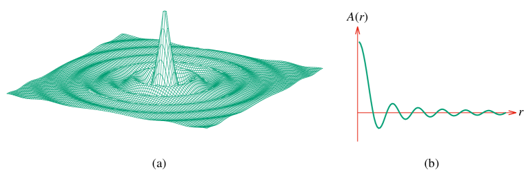
Figure 1: (a) Example of a very intuitive wave phenomenon, but mathematically a slightly complicated one. (b) The one-dimensional cut of this wave shows that the oscillation of this wave is damped.

Since the Schrödinger equation is a differential wave equation, it is essential to remind the students about the wave equation in the classical mechanics. However, it should be remembered that during that time not all students can quickly understand the wave equation in terms of sinusoidal function or differential equation. Therefore, I usually start with the very intuitive wave phenomenon depicted in Fig. 1(a). This phenomenon can be observed if we, e.g., drop a stone in the water. Since the propagation of the wave is radial and the amplitude decreases as the radius increases, the simplest stationary wavefunction reads

$$A(r)=A_{0}\,\frac{\sin r}{r}~{},$$ (1)

where $A(r)$ is the displacement of the water at the position $r$ and $A_{0}$ indicates the amplitude at $r=0$. Note that the wavefunction of the water ripples is actually not stationary, it is a function of time and although we only consider the stationary case given by Eq. (1) it is still not simple. It has a dependence on $r$ in the denominator which is indeed important to suppress the amplitude in the location far from the wave center, as clearly shown by Fig. 1(b).

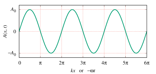
Figure 2: A mathematically simple wave phenomenon, but less intuitive one, i.e., $A(x,t)=A_{0}\,\sin(kx-\omega t)$.

A mathematically much simpler wave equation is the sine wave displayed in Fig. 2. Example of the sine wave is the standing wave observed in the string of a guitar. However, since everybody can easily drop a stone in the water, whereas not everybody has an access to a guitar, the second example is less intuitive. Nevertheless, all students have learned standing wave in high school and since the wave is very simple, we will start our calculation with the sine wave.

The wavefunction displayed in Fig. 2 can be written as

$$A(x,t)=A_{0}\,\sin(kx-\omega t)~{},$$ (2)

where $k$ is the wave number and $\omega$ is the angular frequency. A computer software like Mathematica or Matlab can help the lecturer to simulate this wave during the course. Note that the two parameters define the phase velocity of the wave, i.e.,

$$v=\omega/k~{}.$$ (3)

By taking the second derivatives of Eq. (2) with respect to $x$ and $t$ and using Eq. (3) it is easy to show that

$$\frac{\partial^{2}A(x,t)}{\partial t^{2}}=v^{2}\,\frac{\partial^{2}A(x,t)}{\partial x^{2}}~{}.$$ (4)

Equation (4) is the wave differential equation in classical mechanics. All parameters and variables given in Eq. (4) are real and physical. For instance, the displacement $A(x,t)$ is real and can be observed. For the three dimensional problem this equation is given in the form of the Laplacian operator $\nabla^{2}$, i.e.,

$$\frac{\partial^{2}A({\bf r},t)}{\partial t^{2}}=v^{2}\,\nabla^{2}\,A({\bf r},t)~{}.$$ (5)

Note that, since the cosine function can also describe this wave, it is also possible to generalize the function by using the complex exponential one. It is assumed that students have been acquainted with the imaginary number $i=\sqrt{-1}$ during the calculus course. The general form of Eq. (2) reads

$$A(x,t)=A_{0}\,e^{i(kx-\omega t)}~{}.$$ (6)

The displacement $A(x,t)$ is still observable and real by keeping in mind that the observed quantities are represented by the real and imaginary parts of $A(x,t)$. Here, the imaginary number $i$ works as a unit vector pointing to completely different direction from the real one. Thus, the $i$ number completely separates the sine and cosine waves.

3 Introducing quantum concepts to obtain the Schrödinger equation

Before introducing the Schrödinger equation it is important to explain to students why Schrödinger needed this equation at that time. Therefore, a brief chronological history of this equation is strongly advocated.

We begin with the finding of Max Planck in 1900 which was then proven by Einstein in 1905 that the energy of electromagnetic wave is carried out by the quanta (packets) called photons. Each quantum carries energy of

$$E=h\,\nu~{}=~{}\hbar\,\omega~{},$$ (7)

where $h$ and $\nu$ are the Planck constant and the frequency of the electromagnetic wave, respectively, whereas $\hbar=h/2\pi$. Equation (7) indicates the matter property of a wave, since by using the Einstein energy momentum relation $E^{2}=p^{2}c^{2}+m_{0}^{2}c^{4}$ and remembering that the mass of rest photon is zero, we obtain from Eq. (7) that $pc=hc/\lambda$ or the (matter) momentum of the photon reads

$$p=\frac{h}{\lambda}~{},$$ (8)

where we have used the fact that the speed of electromagnetic wave $c=\lambda\nu$.

In 1924 Louis de Broglie had an idea that in addition to the photon theory of Max Planck and Einstein all particles with momentum $p$, including the massive electrons, have also a wave property with the wavelength of

$$\lambda=\frac{h}{p}~{}.$$ (9)

At first glance Eq. (9) is nothing but Eq. (8). Nevertheless, de Broglie wrote a 73 pages thesis to defense this idea [4]. Even the thesis committee did not know what to to with the thesis, so they sent it to Einstein. Fortunately Einstein saw the point and recommended the approval. Einstein sent the thesis to his colleagues he knew would be interested in the de Broglie’s idea [5].

On November 1925 Erwin Schrödinger attended a colloquium held by his colleague Peter Debye at the E. T. H. Zurich. As noticed by Felix Bloch in his talk given at the 1976 American Physical Society meeting [6] he heard that during the colloquium Debye asked Schrödinger to seriously consider the thesis of de Broglie. What Debye was looking for is actually the wave equation which can properly describe the de Broglie’s wave. As a Sommerfeld student Debye had learned that without wave equation one cannot deal with waves properly. Thus, de Broglie’s thesis was lacked of this equation and Debye challenged Schrödinger to find it. Schrödinger took this challenge during his Christmas vacation and amazingly he was able to submit the result to Annalen der Physik on 27th January 1926 [7].

Let us pretend to be Schrödinger and we accept the Debye’s challenge to find the wave equation. By using Eq. (9) and the relation between wave number and wavelength $k=2\pi/\lambda$, we obtain

$$k=2\pi\,\frac{p}{h}~{}=~{}\frac{p}{\hbar}~{}.$$ (10)

Thus, with the help of Eq. (8) we can recast Eq. (6) into the form

$$\Psi(x,t)=\Psi_{0}\,e^{i(px-Et)/\hbar}~{},$$ (11)

where we have replaced the displacement $A(x,t)$ with $\Psi(x,t)$, along with the amplitude, to indicate that we have included the quantum concept introduced by Max Planck, Einstein, and de Broglie, given by Eqs. (7) and (9), in the wavefunction. In fact, Schrödinger introduced the $\Psi$ function in his equation and called it “a new unknown function” in his 1926 paper [7].

Now, since we are talking about a non-relativistic free particle described by a plane wave, the total energy of the particle is only kinetic energy, i.e., $E=p^{2}/2m$. By using this fact and taking the first derivative of the wavefunction given in Eq. (11) with respect to $t$, as well as the second derivative with respect to $x$, we obtain

$$i\hbar\,\frac{\partial\Psi(x,t)}{\partial t}=-\frac{\hbar^{2}}{2m}\,\frac{\partial^{2}\Psi(x,t)}{\partial x^{2}}~{},$$ (12)

which is the wave equation for a free particle with mass $m$ we are looking for. Since the right hand side of Eq. (12) corresponds to the kinetic energy $T$, we may generalize this equation to describe a particle moving under the influence of a potential energy $V$ and in three dimensional coordinate system as

$$i\hbar\,\frac{\partial\Psi({\bf r},t)}{\partial t}=-\frac{\hbar^{2}}{2m}\,\nabla^{2}\Psi({\bf r},t)+V({\bf r})\,\Psi({\bf r},t)~{},$$ (13)

where we have used the fact that the total energy $E=T+V$. Equation (13) is the Schrödinger equation in general form. We note that similar derivations can be also found in the literature, e.g., Refs. [8, 9, 10, 11].

4 Comparing classical mechanics to quantum mechanics

By introducing the Schrödinger equation in Section 3 we have jumped to the quantum world which is very different from the classical one. At this stage it is important to explain to the students the difference between the classical wave equation given by Eq. (5) and its quantum counterpart given by Eq. (13).

The first and very important difference is the ”displacement” in the two cases. In the classical case the displacement $A({\bf r},t)$ is physical and observable. It is easy to imagine that the water ripples shown in Fig. 1, or the string oscillation displayed in Fig. 2, can be represented by the variation of $A({\bf r},t)$ due to the variations of r and $t$. On the contrary, $\Psi({\bf r},t)$ given in Eq. (13) is not a displacement. It is just a wavefunction describing the de Broglie wave given by Eq. (9).

Is the de Broglie wave physical? Obviously, the answer is no. The massive particles exhibit the wave phenomenon, but the wave itself is not physical. To comprehend this we have to go back to the experimental verification of Eq. (9). The first experiment was performed by Davisson and Germer in 1927 by using electron scattering on a single nickel crystal [12]. A more modern experiment using cold neutrons diffraction on single and double slits was performed by Zeilinger and his collaborators in Grenoble [13]. In principle, it is similar to the conventional diffraction experiment. However, instead of using real photons (visible light) here one uses neutron beams and the general diffraction pattern can be reproduced. Therefore, we may conclude that after passing the slits the neutrons exhibit one of the wave phenomena, i.e., diffraction. This clarifies that we do not detect the de Broglie wave, but we merely observe its phenomenon.

As a consequence, the displacement $A({\bf r},t)$ is real, whereas its counterpart $\Psi({\bf r},t)$ is allowed to be complex function. The latter was actually problematic, even for Schrödinger himself, because he did not expect it. In 1926 Max Born came up with the idea that $\Psi({\bf r},t)$ is a probability amplitude and its modulus squared is the probability density [15], which was considered by Schrödinger with great doubt [6].

The second difference is, unlike the Schrödinger equation, the wave equation is symmetric in the order of derivatives. This explains why the Schrödinger equation is non-relativistic, since it cannot be formulated in a covariant form as in the case of the wave equation for the photons. We know that the covariant formulation requires that both space and time terms should be in the same order.

5 Comparison with other approaches

To the best of my knowledge, there has been no explicit discussion in the literature on the most effective method to introduce the Schrödinger equation during the course of quantum mechanics. However, since most of quantum mechanics textbooks are written based on the teaching experience of the authors, we can compare my approach explained here with the steps used by these authors before they write the Schrödinger equation. Furthermore, the Schrödinger equation is usually introduced in the first or second chapter of quantum mechanics textbooks. Thus, their approaches should be easily identified.

Let us start with the book of Gasiorowicz [14] which has been considered as one of the standard quantum mechanics textbooks used in most universities for relatively long time, i.e., since its first edition in 1974 up to now. In the Sakurai’s book of Modern Quantum Mechanics the editor San Fu Tuan wrote that Gasiorowicz is well known as an effective teacher, who can make difficult concepts simple and clear even in advanced research areas of particle theory [16]. In spite of this great testimony, however, Gasiorowicz introduces the Schrödinger equation abruptly in Chapter 2 in the form of differential equation, without an explanation why we need it. Fortunately, in Chapter 1 Gasiorowicz explains a number of phenomena that indicate the limits of classical physics or the need of quantum mechanics in the beginning of 1900s. Included in these phenomena are the particle behaviour of waves found by Planck and Einstein, and the wave behaviour of particle found by de-Broglie. Nevertheless, since the historical background of quantum mechanics is given in a separate chapter, Gasiorowicz’s step is different from my approach.

The books written by Griffiths are also very popular. Griffiths is well known through his clear and explicit derivations of the used formulas in all of his books. This can be also found in his quantum mechanics book [17]. However, in the case of the Schrödinger equation he also introduced it suddenly on page one and indeed without any historical background. Presumably, Griffiths emphasizes more mathematical formalism than chronological or historical approach. Thus, his approach is also different from mine.

Interestingly, a much older book written by Dicke and Wittke [8] has a much closer approach to the one that I explained in Section 3. Dicke and Wittke open the discussion in Chapter 1 with the evidence of the inadequacy of classical mechanics by explaining Max Planck theory of black-body radiation, theory of specific heats of solids according to Debye, Compton scattering, and their quantum-squirrel-cage gedanken experiment. In Chapter 2 they introduce the de Broglie wave under the name of wave mechanics. In Chapter 3 these authors introduce the Schrödinger equation with a similar step as I explained in Section 3, i.e., they start with Eq. (7) and finish with Eq. (13). After introducing the Schrödinger equation Dicke and Wittke proceed to discuss its solutions for a number of one-dimensional potentials.

More recent and modern quantum mechanics textbooks [18, 19, 20, 21, 22, 23, 24] also introduce the Schrödinger equation abruptly and, in fact, it is mostly in the form of eigenvalue equation $H\Psi=E\Psi$, with $H$ the Hamiltonian of the system. Although most of the books start with historical background of quantum mechanics, it is given in a separate chapter before the one where the Schrödinger equation is introduced. There seems to be an unwritten consensus among these authors that students should have already known the Schrödinger equation as in the case of classical mechanics, in which students have been already very familiar with the Newton laws.

Among the recent quantum mechanics books, only the one written by Steven Weinberg is different [11]. Weinberg opens the book with the first chapter discussing the historical introduction, which is constructed in a chronological order. Indeed, in the beginning of the first chapter Weinberg wrote: ”The principles of quantum mechanics are so contrary to ordinary intuition that they can best be motivated by taking a look at their prehistory.” Thus, in the Weinberg’s book the Schrödinger equation is derived directly in Chapter 1, in a similar manner as the approach given in the present paper.

Another approach which can be contrasted with the one explained in this paper is the original Nuffield A level. We understand that the Nuffield A level is not intended for a rigorous explanation of quantum mechanics. As a consequence, the derivation of Schrödinger equation is most probably beyond the topic of discussion in the Nuffield A level. However, the modern physics part of this approach has been extensively verified. Furthermore, as written by Fuller and Malvern [25] the original Nuffield A Level Physics contains a unit that discusses the quantum mechanics explanation of the wave particle duality phenomenon seriously, i.e., in Unit 10: Waves, Particles and Atoms, which consists of [25]

• photons, wave-particle duality,

• electrons, electrons as a wave,

• waves in boxes, Schödinger’s equation,

• the scope of wave mechanics.

From the ordering of the four items above we may conclude that, in principle, the discussion of Schödinger equation in the original Nuffield A level is in line with my approach explained in this paper.

6 Further consideration

I agree with Steven Weinberg that the best way to introduce quantum mechanics is by considering its chronological history [11]. This include the Schrödinger equation, which is the main equation in non-relativistic quantum mechanics. Nevertheless, to obtain a more objective result a more quantitative investigation should be performed in the class. This can be carried out in two parallel student groups, where two different approaches can be applied. Such an investigation is possible in my physics department, since each semester it runs two or three parallel classes for the Introductory Quantum Mechanics course. Therefore, it is my plan to study the effectiveness of the present approach in the near future.

Having introduced the Schrödinger equation, the next step is presenting the applications of this equation, i.e., variations of the potential $V$ in Eq. (13). Of course, the best example is the application for the Hydrogen atom as described in the Schrödinger paper [7]. However, since simpler is better, I like to start with the traditional approach, i.e., one-dimensional potential. My favorite case here is the simple potential barrier and potential well, which have a wide range of applications, i.e., from scanning tunneling microscope to the nuclear reactions in stars [14]. Such applications have naturally strong impact on the student motivation to attend the course.

7 Summary and Conclusion

I have discussed that introducing the Schrödinger equation during the quantum mechanics course is a critical step, since it constitutes a transition from classical mechanics to the quantum one. Therefore, a smooth but clear transition is required. For this purpose, I used a chronological step in the development of quantum mechanics. I introduced the classical wave equation prior to the quantum one. By using the quantum concepts of the photon energy and the de Broglie wavelength of a moving massive particle I derived the Schrödinger equation following the step to derive the classical wave equation. There are a number of fundamental differences between the two equations, which must be highlighted in order to understand the Schrödinger one and the meaning of the wavefunction $\Psi$. Although the approach explained in this paper is different from those given by most of the authors of quantum mechanics textbooks, it is similar to the approach adopted by Dicke and Wittke, as well as by Steven Weinberg.

References

References

- [1] Feynman R 1965 The Character of Physical Law (Cambridge: The MIT Press) p 129
- [2] Henriksen E K et al2014 Phys. Educ. 49 678
- [3] Michelini M et al2000 Phys. Educ. 35 406
- [4] de Broglie L 1925 Ann. Phys., Paris10 22–128
- [5] Smolin L 2019 Einstein’s unfinished revolution: the search for what lies beyond the quantum (New York: Penguin Press) p 78
- [6] Bloch F 1976 Phys. Today 29 23–7
- [7] Schrödinger E 1926 Ann. Phys., Lpz.384 361–76
- [8] Dicke R H and Wittke J P 1960 Introduction to Quantum Mechanics (Reading, Massachusetts: Addison-Wesley) pp 23–37
- [9] Gorard J 2016 Phys. Educ. 51 063003
- [10] LibreTexts Chemistry Library, available online through https://chem.libretexts.org
- [11] Weinberg S 2015 Lectures on Quantum Mechanics 2nd ed (Cambridge: Cambridge University Press) pp 1–15
- [12] Davisson C and Germer L H 1927 Nature 119, 558–60
- [13] Zeilinger A, Gähler R, Shull C G, Treimer W and Mampe W 1988 Rev. Mod. Phys. 60 1067–73
- [14] Gasiorowicz S 2003 Quantum Physics (New York: John Wiley & Sons) pp 78–89
- [15] Born M 1926 Z. Phys.37 863–7
- [16] Sakurai J J 1985 Modern Quantum Mechanics Tuan S F ed (New York: Addison Wesley Longman) p 489
- [17] Griffiths D J 2005 Introduction to Quantum Mechanics 2nd ed (Upper Saddle River, NJ: Pearson Prentice Hall) p 1
- [18] Auletta G, Fortunato M, and Parisi G 2009 Quantum Mechanics (Cambridge: Cambridge University Press)
- [19] Banks T 2019 Quantum Mechanics: An Introduction (Boca Raton: Taylor & Francis Group)
- [20] Binney J and Skinner D 2014 The Physics of Quantum Mechanics (Oxford: Oxford University Press)
- [21] Commins E D 2014 Quantum Mechanics: an Experimentalist’s Approach (New York: Cambridge University Press)
- [22] McIntyre D H 2012 Quantum Mechanics: a Paradigm Approach (San Francisco: Pearson Education)
- [23] Basdevant J-L and Dalibard J 2002 Quantum Mechanics (Berlin: Springer-Verlag)
- [24] Townsend J S 2012 A Modern Approach to Quantum Mechanics (Mill Valley: University Science Books)
- [25] Fuller K D and Malvern D D 2010 Challenge and Change: a History of the Nuffield A-Level Physics Project (Reading: Institute of Education, University of Reading) available at http://centaur.reading.ac.uk/7534/1/Malvern and Fuller.pdf