Quantum-like modeling in biology with open quantum systems and instruments

Abstract

We present the novel approach to mathematical modeling of information processes in biosystems. It explores the mathematical formalism and methodology of quantum theory, especially quantum measurement theory. This approach is known as quantum-like and it should be distinguished from study of genuine quantum physical processes in biosystems (quantum biophysics, quantum cognition). It is based on quantum information representation of biosystem’s state and modeling its dynamics in the framework of theory of open quantum systems. This paper starts with the non-physicist friendly presentation of quantum measurement theory, from the original von Neumann formulation to modern theory of quantum instruments. Then, latter is applied to model combinations of cognitive effects and gene regulation of glucose/lactose metabolism in Escherichia coli bacterium. The most general construction of quantum instruments is based on the scheme of indirect measurement, in that measurement apparatus plays the role of the environment for a biosystem. The biological essence of this scheme is illustrated by quantum formalization of Helmholtz sensation-perception theory. Then we move to open systems dynamics and consider quantum master equation, with concentrating on quantum Markov processes. In this framework, we model functioning of biological functions such as psychological functions and epigenetic mutation.

keywords: mathematical formalism of quantum mechanics; open quantum systems; quantum instruments; quantum Markov dynamics; gene regulation; psychological effects; cognition; epigenetic mutation; biological functions

1 Introduction

The standard mathematical methods were originally developed to serve classical physics. The real analysis served as the mathematical basis of Newtonian mechanics [1] (and later Hamiltonian formalism); classical statistical mechanics stimulated the measure-theoretic approach to probability theory, formalized in Kolmogorov’s axiomatics [2]. However, behavior of biological systems differ essentially from behavior of mechanical systems, say rigid bodies, gas molecules, or fluids. Therefore, although the “classical mathematics” still plays the crucial role in biological modeling, it seems that it cannot fully describe the rich complexity of biosystems and peculiarities of their behavior – as compared with mechanical systems. New mathematical methods for modeling biosystems are on demand.

In this paper, we present the applications of the mathematical formalism of quantum mechanics and its methodology to modeling biosystems’ behavior. The recent years were characterized by explosion of interest to applications of quantum theory outside of physics, especially in cognitive psychology, decision making, information processing in the brain, molecular biology, genetics and epigenetics, and evolution theory.. We call the corresponding models quantum-like. They are not directed to micro-level modeling of real quantum physical processes in biosystems, say in cells or brains (cf. with with biological applications of genuine quantum physical theory [45]-[52]). Quantum-like modeling works from the viewpoint to quantum theory as a measurement theory. This is the original Bohr’s viewpoint that led to the Copenhagen interpretation of quantum mechanics (see Plotnitsky [53] for detailed and clear presentation of Bohr’s views). One of the main bio-specialties is consideration of self-measurements that biosystems perform on themselves. In our modeling, the ability to perform self-measurements is considered as the basic feature of biological functions (see section 8.2 and paper [54]).

Quantum-like models [17] reflect the features of biological processes that naturally match the quantum formalism. In such modeling, it is useful to explore quantum information theory, which can be applied not just to the micro-world of quantum systems. Generally, systems processing information in the quantum-like manner need not be quantum physical systems; in particular, they can be macroscopic biosystems. Surprisingly, the same mathematical theory can be applied at all biological scales: from proteins, cells and brains to humans and ecosystems; we can speak about quantum information biology [55].

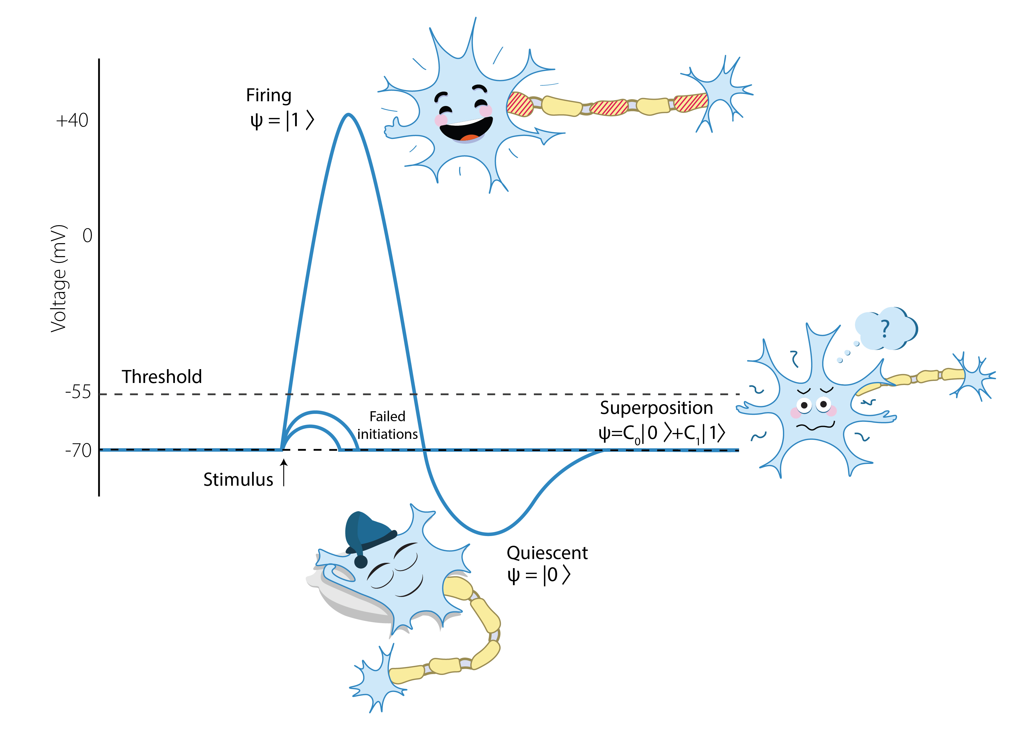
Figure 1: Illustration for quantum-like representation of uncertainty generated by neuron’s action potential (originally published in [54]).

In quantum-like modeling, quantum theory is considered as calculus for prediction and transformation of probabilities. Quantum probability (QP) calculus (section 2) differs essentially from classical probability (CP) calculus based on Kolmogorov’s axiomatics [2]. In CP, states of random systems are represented by probability measures and observables by random variables; in QP, states of random systems are represented by normalized vectors in a complex Hilbert space (pure states) or generally by density operators (mixed states). Superpositions represented by pure states are used to model uncertainty which is yet unresolved by a measurement. The use of superpositions in biology is illustrated by Fig. 1 (see section 10 and paper [54] for the corresponding model). The QP-update resulting from an observation is based on the projection postulate or more general transformations of quantum states - in the framework of theory of quantum instruments [6]-[12] (section 3).

We stress that quantum-like modeling elevates the role of convenience and simplicity of quantum representation of states and observables. (We pragmatically ignore the problem of interrelation of CP and QP.) In particular, the quantum state space has the linear structure and linear models are simpler. Transition from classical nonlinear dynamics of electrochemical processes in biosystems to quantum linear dynamics essentially speeds up the state-evolution (section 8.4). However, in this framework “state” is the quantum information state of a biosystem used for processing of special quantum uncertainty (section 8.2).

In textbooks on quantum mechanics, it is commonly poited out that the main distinguishing feature of quantum theory is the presence of incompatible observables. We recall that two observables, $A$ and $B$ are incompatible if it is impossible to assign values to them jointly. In the probabilistic model, this leads to impossibility to determine their joint probability distribution (JPD). The basic examples of incompatible observables are position and momentum of a quantum system, or spin (or polarization) projections onto different axes. In the mathematical formalism, incompatibility is described as noncommutativity of Hermitian operators $\hat{A}$ and $\hat{B}$ representing observables, i.e., $[\hat{A},\hat{B}]\not=0.$ Here we refer to the original and still basic and widely used model of quantum observables, von Neumann [13] (section 3.2).

Incompatibility-noncommutativity is widely used in quantum physics and the basic physical observables, as say position and momentum, spin and polarization projections, are traditionally represented in this paradigm, by Hermitian operators. Still, it may be not general enough for our purpose - to quantum-like modeling in biology, not any kind of non-classical bio-statistics can be easily delegated to von Neumann model of observations. For example, even very basic cognitive effects cannot be described in a way consistent with the standard observation model [57, 58].

We shall explore more general theory of observations based on quantum instruments [6]-[12] and find useful tools for applications to modeling of cognitive effects [59, 60]. We shall discuss this question in section 3 and illustrate it with examples from cognition and molecular biology in sections 6, 7. In the framework of the quantum instrument theory, the crucial point is not commutativity vs. noncommutativity of operators symbolically representing observables, but the mathematical form of state’s transformation resulting from the back action of (self-)observation. In the standard approach, this transformation is given by an orthogonal projection on the subspace of eigenvectors corresponding to observation’s output. This is the projection postulate. In quantum instrument theory, state transformations are more general.

Calculus of quantum instruments is closely coupled with theory of open quantum systems [14], quantum systems interacting with environments. We remark that in some situations, quantum physical systems can be considered as (at least approximately) isolated. However, biosystems are fundamentally open. As was stressed by Schrödinger [61], a completely isolated biosystem is dead. The latter explains why the theory of open quantum systems and, in particular, the quantum instruments calculus play the basic role in applications to biology, as the mathematical apparatus of quantum information biology [55].

Within theory of open quantum systems, we model epigenetic evolution [epigenetic, 21] (sections 9, 11.2) and performance of psychological (cognitive) functions realized by the brain [63, 21, 54] (sections 10, 11.3).

For mathematically sufficiently well educated biologists, but without knowledge in physics, we can recommend book [56] combining the presentations of CP and QP with a brief introduction to the quantum formalism, including the theory of quantum instruments and conditional probabilities.

2 Classical versus quantum probability

CP was mathematically formalized by Kolmogorov (1933) [2]. This is the calculus of probability measures, where a non-negative weight $p(A)$ is assigned to any event $A.$ The main property of CP is its additivity: if two events $O_{1},O_{2}$ are disjoint, then the probability of disjunction of these events equals to the sum of probabilities:

$$P(O_{1}\vee O_{2})=P(O_{1})+P(O_{2}).$$

QP is the calculus of complex amplitudes or in the abstract formalism complex vectors. Thus, instead of operations on probability measures one operates with vectors. We can say that QP is a vector model of probabilistic reasoning. Each complex amplitude $\psi$ gives the probability by the Born’s rule: Probability is obtained as the square of the absolute value of the complex amplitude.

$$p=|\psi|^{2}$$

(for the Hilbert space formalization, see section 3.2, formula (7)). By operating with complex probability amplitudes, instead of the direct operation with probabilities, one can violate the basic laws of CP.

In CP, the formula of total probability (FTP) is derived by using additivity of probability and the Bayes formula, the definition of conditional probability, $P(O_{2}|O_{1})=\frac{P(O_{2}\cap O_{1})}{P(O_{1})},\;P(O_{1})>0.$ Consider the pair, $A$ and $B,$ of discrete classical random variables. Then

$$P(B=\beta)=\sum_{\alpha}P(A=\alpha)P(B=\beta|A=\alpha).$$

Thus, in CP the $B$-probability distribution can be calculated from the $A$-probability and the conditional probabilities $P(B=\beta|A=\alpha).$

In QP, classical FTP is perturbed by the interference term [19]; for dichotomous quantum observables $A$ and $B$ of the von Neumann-type, i.e., given by Hermitian operators $\hat{A}$ and $\hat{B},$ the quantum version of FTP has the form:

$$P(B=\beta)=\sum_{\alpha}P(A=\alpha)P(B=\beta|a=\alpha)$$ (1)

$$+2\sum_{\alpha_{1}<\alpha_{2}}\cos\theta_{\alpha_{1}\alpha_{2}}\sqrt{P(A=\alpha_{1})P(B=\beta|A=\alpha_{1})P(A=\alpha_{2})P(B=\beta|a=\alpha_{2})}$$ (2)

If the interference term is positive, then the QP-calculus would generate a probability that is larger than its CP-counterpart given by the classical FTP (2). In particular, this probability amplification is the basis of the quantum computing supremacy.

There is a plenty of statistical data from cognitive psychology, decision making, molecular biology, genetics and epigenetics demonstrating that biosystems, from proteins and cells [21] to humans [19, 20] use this amplification and operate with non-CP updates. We continue our presentation with such examples.

3 Quantum instruments

3.1 A few words about the quantum formalism

Denote by ${\cal H}$ a complex Hilbert space. For simplicity, we assume that it is finite dimensional. Pure states of a system $S$ are given by normalized vectors of ${\cal H}$ and mixed states by density operators (positive semi-definite operators with unit trace). The space of density operators is denoted by $\mathbf{S}({\mathcal{H}}).$ The space of all linear operators in ${\cal H}$ is denoted by the symbol ${\cal L}({\cal H}).$ In turn, this is a linear space.Moreover, ${\cal L}({\mathcal{H}})$ is the complex Hilbert space with the scalar product, $\langle A|B\rangle=\rm{Tr}A^{\ast}B.$ We consider linear operators acting in ${\cal L}({\mathcal{H}}).$ They are called superoperators.

The dynamics of the pure state of an isolated quantum system is described by the Schrödinger equation:

$$i\frac{d}{dt}\psi(t)=\hat{H}\psi(t)(t),\;\psi(0)=\psi_{0},$$ (3)

where $\hat{H}$ is system’s Hamiltonian. This equation implies that the pure state $\psi(t)$ evolves unitarily: $\psi(t)=\hat{U}(t)\psi_{0},$ where $\hat{U}(t)=e^{-it\hat{H}}$ is one parametric group of unitary operators, $\hat{U}(t):{\cal H}\to{\cal H}.$ In quantum physics, Hamiltonian $\hat{H}$ is associated with the energy-observable. The same interpretation is used in quantum biophysics [50]. However, in our quantum-like modeling describing information processing in biosystems, the operator $\hat{H}$ has no direct coupling with physical energy. This is the evolution-generator describing information interactions.

Schrödinger’s dynamics for a pure state implies that the dynamics of a mixed state (represented by a density operator) is described by the von Neumann equation:

$$\frac{d\hat{\rho}}{dt}(t)=-i[\hat{H},\hat{\rho}(t)],\;\hat{\rho}(0)=\hat{\rho}_{0}.$$ (4)

3.2 Von Neumann formalism for quantum observables

In the original quantum formalism [13], physical observable $A$ is represented by a Hermitian operator $\hat{A}.$ We consider only operators with discrete spectra: $\hat{A}=\sum_{x}x\;\hat{E}^{A}(x),$ where $\hat{E}^{A}(x)$ is the projector onto the subspace of $H$ corresponding to the eigenvalue $x.$ Suppose that system’s state is mathematically represented by a density operator $\rho.$ Then the probability to get the answer $x$ is given by the Born rule

$$\Pr\{A=x\|\rho\}=\mbox{\rm Tr}[\hat{E}^{A}(x)\rho]=\mbox{\rm Tr}[\hat{E}^{A}(x)\rho\hat{E}^{A}(x)]$$ (5)

and according to the projection postulate the post-measurement state is obtained via the state-transformation:

$$\rho\to\rho_{x}=\frac{\hat{E}^{A}(x)\rho\hat{E}^{A}(x)}{Tr\hat{E}^{A}(x)\rho\hat{E}^{A}(x)}.$$ (6)

For reader’s convenience, we present these formulas for a pure initial state $\psi\in{\cal H}.$ The Born’s rule has the form:

$$\Pr\{A=x\|\rho\}=\|\hat{E}^{A}(x)\psi\|^{2}=\langle\psi|\hat{E}^{A}(x)\psi\rangle.$$ (7)

The state transformation is given by the projection postulate:

$$\psi\to\psi_{x}=\hat{E}^{A}(x)\psi/\|\hat{E}^{A}(x)\psi\|.$$ (8)

Here the observable-operator $\hat{A}$ (its spectral decomposition) uniquely determines the feedback state transformations ${\mathcal{I}}_{A}(x)$ for outcomes $x$

$$\rho\to{\mathcal{I}}_{A}(x)\rho=\hat{E}^{A}(x)\rho\hat{E}^{A}(x).$$ (9)

The map $x\to{\mathcal{I}}_{A}(x)$ given by (9) is the simplest (but very important) example of quantum instrument.

3.3 Non-projective state update: atomic instruments

In general, the statistical properties of any measurement are characterized by

• the output probability distribution $\Pr\{\mathbf{x}=x\|\rho\}$, the probability distribution of the output $\mathbf{x}$ of the measurement in the input state $\rho$;

• the quantum state reduction $\rho\mapsto\rho_{\{\mathbf{x}=x\}}$, the state change from the input state $\rho$ to the output state $\rho_{\{\mathbf{x}=x\}}$ conditional upon the outcome $\mathbf{x}=x$ of the measurement.

In von Neumann’s formulation, the statistical properties of any measurement of an observable $A$ is uniquely determined by Born’s rule (5) and the projection postulate (6), and they are represented by the map (9), an instrument of von Neumann type. However, von Neumann’s formulation does not reflect the fact that the same observable $A$ represented by the Hermitian operator $\hat{A}$ in ${\mathcal{H}}$ can be measured in many ways. Formally, such measurement-schemes are represented by quantum instruments.

Now, we consider the simplest quantum instruments of non von Neumann type, known as atomic instruments. We start with recollection of the notion of POVM (probability operator valued measure); we restrict considerations to POVMs with a discrete domain of definition $X=\{x_{1},...,x_{N},...\}$. POVM is a map $x\to\hat{D}(x)$ such that for each $x\in X,$ $\hat{D}(x)$ is a positive contractive Hermitian operator (called effect) (i.e., $\hat{D}(x)^{\ast}=\hat{D}(x)$, $0\leq\langle\psi|\hat{D}(x)\psi\rangle\leq 1$ for any $\psi\in{\cal H}$), and the normalization condition

$$\sum_{x}\hat{D}(x)=I$$

holds, where $I$ is the unit operator. It is assumed that for any measurement, the output probability distribution $\Pr\{\mathbf{x}=x\|\rho\}$ is given by

$$\Pr\{\mathbf{x}=x\|\rho\}=\mbox{\rm Tr}[\hat{D}(x)\rho],$$ (10)

where $\{\hat{D}(x)\}$ is a POVM. For atomic instruments, it is assumed that effects are represented concretely in the form

$$\hat{D}(x)=\hat{V}(x)^{\ast}\hat{V}(x),$$ (11)

where $V(x)$ is a linear operator in $H.$ Hence, the normalization condition has the form $\sum_{x}V(x)^{\ast}V(x)=I.$ The Born rule can be written similarly to (5):

$$\Pr\{\mathbf{x}=x\|\rho\}=\mbox{\rm Tr}[V(x)\rho V^{\ast}(x)]$$ (12)

It is assumed that the post-measurement state transformation is based on the map:

$$\rho\to{\mathcal{I}}_{A}(x)\rho=V(x)\rho V^{\ast}(x),$$ (13)

so the quantum state reduction is given by

$$\rho\to\rho_{\{\mathbf{x}=x\}}=\frac{{\mathcal{I}}_{A}(x)\rho}{\mbox{\rm Tr}[{\mathcal{I}}_{A}(x)\rho]}.$$ (14)

The map $x\to{\mathcal{I}}_{A}(x)$ given by (13) is an atomic quantum instrument. We remark that the Born rule (12) can be written in the form

$$\Pr\{\mathbf{x}=x\|\rho\}=\mbox{\rm Tr}\;[{\mathcal{I}}_{A}(x)\rho].$$ (15)

Let $\hat{A}$ be a Hermitian operator in ${\mathcal{H}}.$ Consider a POVM $\hat{D}=(\hat{D}^{A}(x))$ with the domain of definition given by the spectrum of $\hat{A}.$ This POVM represents a measurement of observable $A$ if Born’s rule holds:

$$\Pr\{A=x\|\rho\}=\mbox{\rm Tr}[\hat{D}^{A}(x)\rho]=\mbox{\rm Tr}[\hat{E}^{A}(x)\rho].$$ (16)

Thus, in principle, probabilities of outcomes are still encoded in the spectral decomposition of operator $\hat{A}$ or in other words operators $\hat{D}^{A}(x)$ should be selected in such a way that they generate the probabilities corresponding to the spectral decomposition of the symbolic representation $\hat{A}$ of observables $A$, i.e., $\hat{D}^{A}(x)$ is uniquely determined by $\hat{A}$ as $\hat{D}^{A}(x)=\hat{E}^{A}(x)$. We can say that this operator carries only information about the probabilities of outcomes, in contrast to the von Neumann scheme, operator $\hat{A}$ does not encode the rule of the state update. For an atomic instrument, measurements of the observable $A$ has the unique output probability distribution by the Born’s rule (16), but has many different quantum state reductions depending of the decomposition of the effect $\hat{D}(x)=\hat{E}^{A}(x)=V(x)^{*}V(x)$ in such a way that

$$\rho\to\rho_{\{A=x\}}=\frac{V(x)\rho V(x)^{*}}{\mbox{\rm Tr}[V(x)\rho V(x)^{*}]}.$$ (17)

3.4 General theory (Davies–Lewis-Ozawa)

Finally, we formulate the general notion of quantum instrument. A superoperator acting in ${\cal L}({\cal H})$ is called positive if it maps the set of positive semi-definite operators into itself. We remark that, for each $x,$ ${\mathcal{I}}_{A}(x)$ given by (13) can be considered as linear positive map.

Generally any map $x\to{\mathcal{I}}_{A}(x),$ where for each $x,$ the map ${\mathcal{I}}_{A}(x)$ is a positive superoperator is called Davies–Lewis [6] quantum instrument. Here index $A$ denotes the observable coupled to this instrument. The probabilities of $A$-outcomes are given by Born’s rule in form (15) and the state-update by transformation (14). However, Yuen [9] pointed out that the class of Davies–Lewis instruments is too general to exclude physically non-realizable instruments. Ozawa [8] introduced the important additional condition to ensure that every quantum instrument is physically realizable. This is the condition of complete positivity. A superoperator is called completely positive if its natural extension ${\cal T}\otimes I$ to the tensor product ${\cal L}({\mathcal{H}})\otimes{\cal L}({\mathcal{H}})={\cal L}({\mathcal{H}}\otimes{\mathcal{H}})$ is again a positive superoperator on ${\cal L}({\mathcal{H}})\otimes{\cal L}({\mathcal{H}}).$ A map $x\to{\mathcal{I}}_{A}(x),$ where for each $x,$ the map ${\mathcal{I}}_{A}(x)$ is a completely positive superoperator is called Davies-Lewis-Ozawa [6, 8] quantum instrument or simply quantum instrument. As we shall see in section 4, complete positivity is a sufficient condition for an instrument to be physically realizable. On the other hand, necessity is derived as follows [11]. Every observable $A$ of a system $S$ is identified with the observable $A\otimes I$ of a system $S+S^{\prime}$ with any system $S^{\prime}$ external to $S.$ Then, every physically realizable instrument ${\cal I}_{A}$ measuring $A$ should be identified with the instrument ${\cal I}_{A\otimes I}$ measuring $A\otimes I$ such that ${\cal I}_{A\otimes I}(x)={\cal I}_{A}(x)\otimes I$. This implies that ${\cal I}_{A}(x)\otimes I$ is agin a positive superoperator, so that ${\cal I}_{A}(x)$ is completely positive. Similarly, any physically realizable instrument ${\mathcal{I}}_{A}(x)$ measuring system $S$ should have its extended instrument ${\mathcal{I}}_{A}(x)\otimes I$ measuring system $S+S^{\prime}$ for any external system $S^{\prime}$. This is fulfilled only if ${\mathcal{I}}_{A}(x)$ is completely positive. Thus, complete positivity is a necessary condition for ${\cal I}_{A}$ to describe a physically realizable instrument.

4 Quantum instruments from the scheme of indirect measurements

The basic model for construction of quantum instruments is based on the scheme of indirect measurements. This scheme formalizes the following situation: measurement’s outputs are generated via interaction of a system $S$ with a measurement apparatus $M.$ This apparatus consists of a complex physical device interacting with $S$ and a pointer that shows the result of measurement, say spin up or spin down. An observer can see only outputs of the pointer and he associates these outputs with the values of the observable $A$ for the system $S.$ S Thus, the indirect measurement scheme involves:

• the states of the systems $S$ and the apparatus $M;$

• the operator $U$ representing the interaction-dynamics for the system $S+M;$

• the meter observable $M_{A}$ giving outputs of the pointer of the apparatus $M.$

An indirect measurement model, introduced in [8] as a “(general) measuring process”, is a quadruple

$$({\mathcal{K}},\sigma,U,M_{A})$$

consisting of a Hilbert space ${\mathcal{K}},$ a density operator $\sigma\in{\bf S}({\mathcal{K}}),$ a unitary operator $U$ on the tensor product of the state spaces of $S$ and $M,$ $U:{\mathcal{H}}\otimes{\mathcal{K}}\to{\mathcal{H}}\otimes{\mathcal{K}},$ and a Hermitian operator $M_{A}$ on ${\mathcal{K}}$. By this measurement model, the Hilbert space ${\mathcal{K}}$ describes the states of the apparatus $M$, the unitary operator $U$ describes the time-evolution of the composite system $S+M$, the density operator $\sigma$ describes the initial state of the apparatus $M$, and the Hermitian operator $M_{A}$ describes the meter observable of the apparatus $M.$ Then, the output probability distribution $\Pr\{A=x\|\rho\}$ in the system state $\rho\in\bf{S}({\mathcal{H}})$ is given by

$$\Pr\{A=x\|\rho\}=\mbox{\rm Tr}[(I\otimes E^{M_{A}}(x))U(\rho\otimes\sigma)U^{\ast}],$$ (18)

where $E^{M_{A}}(x)$ is the spectral projection of $M_{A}$ for the eigenvalue $x.$

The change of the state $\rho$ of the system $S$ caused by the measurement for the outcome $A=x$ is represented with the aid of the map ${\mathcal{I}}_{A}(x)$ in the space of density operators defined as

$${\mathcal{I}}_{A}(x)\rho=\mbox{\rm Tr}_{{\mathcal{K}}}[(I\otimes E^{M_{A}}(x))U(\rho\otimes\sigma)U^{\ast}],$$ (19)

where $\mbox{\rm Tr}_{{\mathcal{K}}}$ is the partial trace over ${\mathcal{K}}.$ Then, the map $x\mapsto{\mathcal{I}}_{A}(x)$ turn out to be a quantum instrument. Thus, the statistical properties of the measurement realized by any indirect measurement model $({\mathcal{K}},\sigma,U,M_{A})$ is described by a quantum measurement. We remark that conversely any quantum instrument can be represented via the indirect measurement model [8]. Thus, quantum instruments mathematically characterize the statistical properties of all the physically realizable quantum measurements.

5 Modeling of the process of sensation-perception within indirect measurement scheme

Foundations of theory of unconscious inference for the formation of visual impressions were set in 19th century by H. von Helmholtz. Although von Helmholtz studied mainly visual sensation-perception, he also applied his theory for other senses up to culmination in theory of social unconscious inference. By von Helmholtz here are two stages of the cognitive process, and they discriminate between sensation and perception as follows:

• Sensation is a signal which the brain interprets as a sound or visual image, etc.

• Perception is something to be interpreted as a preference or selective attention, etc.

In the scheme of indirect measurement, sensations represent the states of the sensation system $S$ of human and the perception system plays the role of the measurement apparatus $M.$ The unitary operator $U$ describes the process of interaction between the sensation and perception states. This quantum modeling of the process of sensation-perception was presented in paper [65] with application to bistable perception and experimental data from article [66].

6 Modeling of cognitive effects

In cognitive and social science, the following opinion pool is known as the basic example of the order effect. This is the Clinton-Gore opinion pool [67]. In this experiment, American citizens were asked one question at a time, e.g.,

• $A$ = “Is Bill Clinton honest and trustworthy?”

• $B$ = “Is Al Gore honest and trustworthy?”

Two sequential probability distributions were calculated on the basis of the experimental statistical data, $p_{AB}$ and $p_{BA}$ (first question $A$ and then question $B$ and vice verse).

6.1 Order effect for sequential questioning

The statistical data from this experiment demonstrated the question order effect QOE, dependence of sequential joint probability distribution for answers to the questions on their order: $p_{AB}\not=p_{BA}.$ We remark that in the CP-model these probability distributions coincide: $p_{AB}(\alpha,\beta)=P(\omega\in\Omega:A(\omega)=\alpha,B(\omega)=\beta)=p_{BA}(\beta,\alpha),$ where $\Omega$ is a sample space and $P$ is a probability measure. QOE stimulates application of the QP-calculus to cognition, see paper [29]. The authors of this paper stressed that noncommutative feature of joint probabilities can be modeled by using noncommutativity of incompatible quantum observables $A,B$ represented by Hermitian operators $\hat{A},\hat{B}.$ Observable $A$ represents the Clinton-question and observable $B$ represents Gore-question. In this model, QOE is identical incompatibility-noncommutativity of observables: $[\hat{A},\hat{B}]\not=0.$

6.2 Response replicability effect for sequential questioning

The approach based on identification of the order effect with noncommutative representation of questions [29] was criticized in paper [57]. To discuss this paper, we recall the notion of response replicability. Suppose that a person, say John, is asked some question $A$ and suppose that he replies, e,g, “yes”. If immediately after this, he is asked the same question again, then he replies “yes” with probability one. We call this property $A-A$ response replicability. In quantum physics, $A-A$ response replicability is expressed by the projection postulate. The Clinton-Gore opinion poll as well as typical decision making experiments satisfy $A-A$ response replicability. Decision making has also another feature - $A-B-A$ response replicability. Suppose that after answering the $A$-question with say the “yes”-answer, John is asked another question $B.$ He replied to it with some answer. And then he is asked $A$ again. In the aforementioned social opinion pool, John repeats her original answer to $A,$ “yes” (with probability one). This behavioral phenomenon we call $A-B-A$ response replicability. Combination of $A-A$ with $A-B-A$ and $B-A-B$ response replicability is called the response replicability effect RRE.

6.3 “QOE+RRE”: described by quantum instruments of non-projective type

In paper [57], it was shown that by using the von Neumann calculus it is impossible to combine RRE with QOE. To generate QOE, Hermitian operators $\hat{A},\hat{B}$ should be noncommutative, but the latter destroys$A-B-A$ response replicability of $A.$ This was a rather unexpected result. It made even impression that, although the basic cognitive effects can be quantum-likely modeled separately, their combinations cannot be described by the quantum formalism.

However, recently it was shown that theory of quantum instruments provides a simple solution of the combination of QOE and RRE effects, see [59] for construction of such instruments. These instruments are of non-projective type. Thus, the essence of QOE is not in the structure of observables, but in the structure of the state transformation generated by measurements’ feedback. QOE is not about the joint measurement and incompatibility (noncommutativity) of observables, but about sequential measurement of observables and sequential (mental-)state update. Quantum instruments which are used in [59] to combine QOE and RRE correspond to measurement of observables represented by commuting operators $\hat{A},\hat{B}.$ Moreover, it is possible to prove that (under natural mathematical restriction) QOE and RRE can be jointly modeled only with the aid of quantum instruments for commuting observables.

6.4 Mental realism

Since very beginning of quantum mechanics, noncommutativity of operators $\hat{A},\hat{B}$ representing observables $A,B$ was considered as the mathematical representation of their incompatibility. In philosophic terms, this situation is treated as impossibility of the realistic description. In cognitive science, this means that there exist mental states such that an individual cannot assign the definite values to both observables (e.g., questions). The mathematical description of QOE with observables represented by noncommutative operators (in the von Neumann’s scheme) in [29, 30] made impression that this effect implies rejection of mental realism. The result of [59] demonstrates that, in spite of experimentally well documented QOE, the mental realism need not be rejected. QOE can be modeled within the realistic picture mathematically given by the joint probability distribution of observables $A$ and $B,$ but with the noncommutative action of quantum instruments updating the mental state:

$$[{\mathcal{I}}_{A}(x),{\mathcal{I}}_{B}(x)]={\mathcal{I}}_{A}(x){\mathcal{I}}_{B}(x)-{\mathcal{I}}_{B}(x){\mathcal{I}}_{A}(x)\not=0.$$ (20)

This is the good place to remark that if, for some state $\rho,[{\mathcal{I}}_{A}(x),{\mathcal{I}}_{B}(x)]\rho=0,$ then QOE disappears, even if $[{\mathcal{I}}_{A}(x),{\mathcal{I}}_{B}(x)]\not=0.$ This can be considered as the right formulation of Wang-Bussemeyer statement on connection of QOE with noncommutativity. Instead of noncommutativity of operators $\hat{A}$ and $\hat{B}$ symbolically representing quantum obseravbles, one has to speak about noncommutativity of corresponding quantum instruments.

7 Genetics: interference in glucose/lactose metabolism

In paper [64], there was developed a quantum-like model describing the gene regulation of glucose/lactose metabolism in Escherichia coli bacterium. There are several types of E. coli characterized by the metabolic system. It was demonstrated that the concrete type of E. coli can be described by the well determined linear operators; we find the invariant operator quantities characterizing each type. Such invariant operator quantities can be calculated from the obtained statistical data. So, the quantum-like representation was reconstructed from experimental data.

Let us consider an event system $\{Q_{+},Q_{-}\}:Q_{+}$ means the event that E. coli activates its lactose operon, that is, the event that $\beta$-galactosidase is produced through the transcription of mRNA from a gene in lactose operon; $Q_{-}$ means the event that E. coli does not activates its lactose operon. This system of events corresponds to activation observable $Q$ that is mathematically represented by a quantum instrument ${\cal T}_{Q}.$ Consider now another system of events $\{D_{L},D_{G}\}$ where $D_{L}$ means the event that an E. coli bacterium detects a lactose molecular in cell’s surrounding environment, $D_{G}$ means detection of a glucose molecular. This system of events corresponds to detection observable $D$ that is represented by a quantum instrument ${\cal T}_{D}.$ In this model, bacterium’s interaction-reaction with glucose/lactose environment is described as sequential action of two quantum instruments, first detection and then activation. As was shown in [64], for each concrete type of E. coli bacterium, these quantum instruments can be reconstructed from the experimental data; in [64], reconstruction was performed for W3110-type of E. coli bacterium. The classical FTP with observables $A=D$ and $B=Q$ is violated, the interference term, see (2), was calculated [64].

8 Open quantum systems: interaction of a biosystem with its environment

As was already emphasized, any biosystem $S$ is fundamentally open. Hence, dynamics of its state has to be modeled via an interaction with surrounding environment ${\cal E}.$ The states of $S$ and ${\cal E}$ are represented in the Hilbert spaces ${\mathcal{H}}$ and ${\mathcal{K}}.$ The compound system $S+{\cal E}$ is represented in the tensor product Hilbert spaces ${\mathcal{H}}\otimes{\mathcal{K}}.$ This system is treated as an isolated system and in accordance with quantum theory, dynamics of its pure state can be described by the Schrödinger equation:

$$i\frac{d}{dt}\Psi(t)=\hat{H}\Psi(t)(t),\;\Psi(0)=\Psi_{0},$$ (21)

where $\Psi(t)$ is the pure state of the system $S+{\cal E}$ and $\hat{H}$ is its Hamiltonian. This equation implies that the pure state $\psi(t)$ evolves unitarily : $\Psi(t)=\hat{U}(t)\Psi_{0},$ where $\hat{U}(t)=e^{-it\hat{H}}.$ Hamiltonian, the evolution-generator, describing information interactions has the form $\hat{H}=\hat{H}_{S}+\hat{H}_{{\cal E}}+\hat{H}_{S,{\cal E}},$ where $\hat{H}_{S},\hat{H}_{{\cal E}}$ are Hamiltonians of the systems and $\hat{H}_{S,{\cal E}}$ is the interaction Hamiltonian. This equation implies that evolution of the density operator $\hat{R}(t)$ of the system $S+{\cal E}$ is described by von Neumann equation:

$$\frac{d\hat{R}}{dt}(t)=-i[\hat{H},\hat{R}(t)],\;\hat{R}(0)=\hat{R}_{0},$$ (22)

However, the state $\hat{R}(t)$ is too complex for any mathematical analysis: the environment includes too many degrees of freedom. Therefore, we are interested only the state of $S;$ its dynamics is obtained via tracing of the state of $S+{\cal E}$ w.r.t. the degrees of freedom of ${\cal E}:$

$$\hat{\rho}(t)=\rm{Tr}_{{\mathcal{K}}}\hat{R}(t).$$ (23)

Generally this equation, the quantum master equation, is mathematically very complicated. A variety of approximations is used in applications.

8.1 Quantum Markov model: Gorini-Kossakowski-Sudarshan-Lindblad equation

The simplest approximation of quantum master equation (23) is the quantum Markov dynamics given by the Gorini-Kossakowski-Sudarshan-Lindblad (GKSL) equation [14] (in physics, it is commonly called simply the Lindblad equation; this is the simplest quantum master equation):

$$\frac{d\hat{\rho}}{dt}(t)=-i[\hat{H},\hat{\rho}(t)]+\hat{L}[\hat{\rho}(t)],\;\hat{\rho}(0)=\hat{\rho}_{0},$$ (24)

where Hermitian operator (Hamiltonian) $\hat{H}$ describes the internal dynamics of $S$ and the superoperator $\hat{L},$ acting in the space of density operators, describes an interaction with environment ${\cal E}.$ This superoperator is often called Lindbladian. The GKSL-equation is a quantum master equation for Markovian dynamics. In this paper, we have no possibility to explain the notion of quantum Markovianity in more detail. Quantum master equation (23) describes generally non-Markovean dynamics.

8.2 Biological functions in the quantum Markov framework

We turn to the open system dynamics with the GKSL-equation. In our modeling, Hamiltonian $\hat{H}$ and Lindbladian $\hat{L}$ represent some special biological function $F$ (see [54]) for details. Its functioning results from interaction of internal and external information flows. In sections 10, 11.3, $F$ is some psychological function; in the simplest case $F$ represents a question asked to $S$ (say $S$ is a human being). In section 7, $F$ is the gene regulation of glucose/lactose metabolism in Escherichia coli bacterium. In sections 9, 11.2, $F$ represents the process of epigenetic mutation. Symbolically biological function $F$ is represented as a quantum observable: Hermitian operator $\hat{F}$ with the spectral decomposition $\hat{F}=\sum_{x}x\hat{E}^{F}(x),$ where $x$ labels outputs of $F.$ Theory of quantum Markov state-dynamics describes the process of generation of these outputs.

In the mathematical model [21, AS3, 41, 55, epigenetic, 63, 64], the outputs of biological function $F$ are generated via approaching a steady state of the GKSL-dynamics:

$$\lim_{t\to\infty}\hat{\rho}(t)=\hat{\rho}_{\rm{steady}}$$ (25)

such that it matches the spectral decomposition of $\hat{F},$ i.e.,

$$\hat{\rho}_{\rm{steady}}=\sum_{x}p_{x}\hat{E}^{F}(x),\;\mbox{where}\;p_{x}\geq 0,\sum_{x}p_{x}=1.$$ (26)

This means that $\hat{\rho}_{\rm{steady}}$ is diagonal in an orthonormal basis consisting of eigenvectors of $\hat{F}.$ This state, or more precisely, this decomposition of density operator $\hat{\rho}_{\rm{steady}}$, is the classical statistical mixture of the basic information states determining this biological function. The probabilities in state’s decomposition (26) are interpreted statistically.

Consider a large ensemble of biosystems with the state $\hat{\rho}_{0}$ interacting with environment ${\cal E}.$ (We recall that mathematically the interaction is encoded in the Lindbladian $\hat{L}.)$ Resulting from this interaction, biological function $F$ produces output $x$ with probability $p_{x}.$ We remark that in the operator terms the probability is expressed as $p_{x}=\rm{Tr}\hat{\rho}_{\rm{steady}}\hat{E}^{F}(x).$ This interpretation can be applied even to a single biosystem that meets the same environment many times.

It should be noted that limiting state $\hat{\rho}_{\rm{steady}}$ expresses the stability with respect to the influence of concrete environment ${\cal E}.$ Of course, in the real world the limit-state would be never approached. The mathematical formula (25) describes the process of stabilization, damping of fluctuations. But, they would be never disappear completely with time.

We note that a steady state satisfies the stationary GKSL-equation:

$$i[\hat{H},\hat{\rho}_{\rm{steady}}]=\hat{L}[\hat{\rho}_{\rm{steady}}].$$ (27)

It is also important to point that generally a steady state of the quantum master equation is not unique, it depends on the class of initial conditions.

8.3 Operation of biological functions through decoherence

To make the previous considerations concrete, let us consider a pure quantum state as the initial state. Suppose that a biological function $F$ is dichotomous, $F=0,1,$ and it is symbolically represented by the Hermitian operator that is diagonal in orthonormal basis $|0\rangle,|1\rangle.$ (We consider the two dimensional state space - the qubit space.) Let the initial state has the form of superposition

$$|\psi\rangle=c_{0}|0\rangle+c_{1}|1\rangle,$$ (28)

where $c_{j}\in\mathbf{C},|c_{0}|^{2}+|c_{1}|^{2}=1.$ The quantum master dynamics is not a pure state dynamics: sooner or later (in fact, very soon), this superposition representing a pure state will be transferred into a density matrix representing a mixed state. Therefore, from the very beginning it is useful to represent superposition (28) in terms of a density matrix:

$$\hat{\rho}_{0}=\begin{vmatrix}|c_{0}|^{2}&c_{0}\bar{c}_{1}\\ \bar{c}_{0}c_{1}&|c_{1}|^{2}\\ \end{vmatrix}$$ (29)

State’s purity, superposition, is characterized by the presence of nonzero off-diagonal terms.

Superposition encodes uncertainty with respect to the concrete state basis, in our case $|0\rangle,|1\rangle.$ Initially biological function $F$ was in the state of uncertainty between two choices $x=0,1.$ This is genuine quantum(-like) uncertainty. Uncertainty, about possible actions in future. For example, for psychological function (section 10) $F$ representing answering to some question, say “to buy property” ($F=1)$ and its negation ($F=0),$ a person whose state is described by superposition (28) is uncertain to act with $F=1$ or with $F=0.$ Thus, a superposition-type state describes individual uncertainty, i.e., uncertainty associated with the individual biosystem and not with an ensemble of biosystems; with the single act of functioning of $F$ and not with a large series of such acts.

Resolution of uncertainty with respect to $\hat{F}$-basis is characterized by washing off the off-diagonal terms in (29) The quantum dynamics (24) suppresses the off-diagonal terms and, finally, a diagonal density matrix representing a steady state of this dynamical systems is generated:

$$\hat{\rho}_{\rm{steady}}=\begin{vmatrix}p_{0}&0\\ 0&p_{1}\\ \end{vmatrix}$$ (30)

This is a classical statistical mixture. It describes an ensemble of biosystems; statistically they generate outputs $F=\alpha$ with probabilities $p_{\alpha}.$ In the same way, the statistical interpretation can be used for a single system that performs $F$-functioning at different instances of time (for a long time series).

In quantum physics, the process of washing off the off-diagonal elements in a density matrix is known as the process of decoherence. Thus, the described model of can be called operation of biological function through decoherence.

8.4 Linearity of quantum representation: exponential speed up for biological functioning

The quantum-like modeling does not claim that biosystems are fundamentally quantum. A more natural picture is that they are a complex classical biophysical systems and the quantum-like model provides the information representation of classical biophysical processes, in genes, proteins, cells, brains. One of the advantages of this representation is its linearity. The quantum state space is a complex Hilbert space and dynamical equations are linear differential equations. For finite dimensional state spaces, these are just ordinary differential equations with complex coefficients (so, the reader should not be afraid of such pathetic names as Schrödinger, von Neumann, or Gorini-Kossakowski-Sudarshan-Lindblad equations). The classical biophysical dynamics beyond the quantum information representation is typically nonlinear and very complicated. The use of the linear space representation simplifies the processing structure. There are two viewpoints on this simplification, external and internal. The first one is simplification of mathematical modeling, i.e., simplification of study of bioprocesses (by us, external observers). The second one is more delicate and interesting. We have already pointed to one important specialty of applications of the quantum theory to biology. Here, systems can perform self-observations. So, in the process of evolution say a cell can “learn” via such self-observations that it is computationally profitable to use the linear quantum-like representation. And now, we come to the main advantage of linearity. The linear dynamics exponentially speeds up information processing. Solutions of the GKSL-equation can be represented in the form $\hat{\rho}(t)=e^{t\hat{\Gamma}}\hat{\rho}_{0},$ where $\hat{\Gamma}$ is the superoperator given by the right-hand side of the GKSL-equation. In the finite dimensional case, decoherence dynamics is expressed via factors of the form $e^{t(ia-b)},$ where $b>0.$ Such factors are exponentially decreasing. Quantum-like linear realization of biological functions is exponentially rapid comparing with nonlinear classical dynamics.

The use of the quantum information representation means that generally large clusters of classical biophysical states are encoded by a few quantum states. It means huge information compressing. It also implies increasing of stability in state-processing. Noisy nonlinear classical dynamics is mapped to dynamics driven by linear quantum(-like) equation of say GKSL-type. The latter has essentially simpler structure and via selection of the operator coefficients encoding symbolically interaction within the system $S$ and with its surrounding environment ${\cal E},$ $S$ can establish dynamics with stabilization regimes leading to steady states.

9 Epigenetic evolution within theory of open quantum systems

In paper [epigenetic], a general model of the epigenetic evolution unifying neo-Darwinian with neo-Lamarckian approaches was created in the framework of theory of open quantum systems. The process of evolution is represented in the form of adaptive dynamics given by the quantum(-like) master equation describing the dynamics of the information state of epigenome in the process of interaction with surrounding environment. This model of the epigenetic evolution expresses the probabilities for observations which can be done on epigenomes of cells; this (quantum-like) model does not give a detailed description of cellular processes. The quantum operational approach provides a possibility to describe by one model all known types of cellular epigenetic inheritance.

To give some hint about the model, we consider one gene, say $g.$ This is the system $S$ in section 8.1. It interacts with the surrounding environment ${\cal E}:$ a cell containing this gene and other cells that send signals to this concrete cell and through it to the gene $g.$ As a consequence of this interaction some epigenetic mutation $\mu$ in the gene $g$ can happen. It would change the level of the $g$-expression. For the moment, we ignore that there are other genes. In this oversimplified model, the mutation can be described within the two dimensional state space, complex Hilbert space ${\cal H}_{\rm{epi}}$ (qubit space). States of $g$ without and with mutation are represented by the orthogonal basis $|0\rangle,|1\rangle;$ these vectors express possible epigenetic changes of the fixed type $\mu.$ A pure quantum information state has the form of superposition $|\psi_{\rm{epi}}\rangle=c_{0}|0\rangle+c_{1}|1\rangle.$ Now, we turn to the general scheme of section 8.2 with the biological function $F$ expressing $\mu$-epimutation in one fixed gene. The quantum Markov dynamics (24) resolves uncertainty encoded in superposition $|\psi_{\rm{epi}}\rangle$ (“modeling epimutations as decoherence”). The classical statistical mixture $\rho_{\rm{steady}},$ see (30), is approached. Its diagonal elements $p_{0},p_{1}$ give the probabilities of the events: “no $\mu$-epimutation” and “$\mu$-epimutation”. These probabilities are interpreted statistically: in a large population of cells, $M$ cells, $M\gg 1,$, the number of cells with $\mu$-epimutation is $N_{m}\approx p_{1}M.$ This $\mu$-epimutation in a cell population would stabilize completely to the steady state only in the infinite time. Therefore in reality there are fluctuations (of decreasing amplitude) in any finite interval of time.

Finally, we point to the advantage of the quantum-like dynamics of interaction of genes with environment - dynamics’ linearity implying exponential speed up of the process of epigenetic evolution (section 8.4).

10 Connecting electrochemical processes in neural networks with quantum informational processing

As was emphasized in introduction, quantum-like models are formal operational models describing information processing in biosystems. (in contrast to studies in quantum biology - the science about the genuine quantum physical processes in biosystems). Nevertheless, it is interesting to connect the structure quantum information processing in a biosystem with physical and chemical processes in it. This is a problem of high complexity. Papers [54] present the attempt to proceed in this direction for the human brain - the most complicated biosystem (and at the same time the most interesting for scientists). In the framework of quantum information theory, there was modeled information processing by brain’s neural networks. The quantum information formalization of the states of neural networks is coupled with the electrochemical processes in the brain. The key-point is representation of uncertainty generated by the action potential of a neuron as quantum(-like) superposition of the basic mental states corresponding to a neural code, see Fig. 1 for illustration.

Consider information processing by a single neuron; this is the system $S$ (see section 8.2). Its quantum information state corresponding to the neural code quiescent and firing, 0/1, can be represented in the two dimensional complex Hilbert space ${\cal H}_{\rm{neuron}}$ (qubit space). At a concrete instant of time neuron’s state can be mathematically described by superposition of two states, labeled by $|0\rangle,|1\rangle:$ $|\psi_{\rm{neuron}}\rangle=c_{0}|0\rangle+c_{1}|1\rangle.$ It is assumed that these states are orthogonal and normalized, i.e., $\langle 0|1\rangle=0$ and $\langle\alpha|\alpha\rangle=1,\alpha=0,1.$ The coordinates $c_{0}$ and $c_{1}$ with respect to the quiescent-firing basis are complex amplitudes representing potentialities for the neuron $S$ to be quiescent or firing. Superposition represents uncertainty in action potential, “to fire” or “not to fire”. This superposition is quantum information representation of physical, electrochemical uncertainty.

Let $F$ be some psychological (cognitive) function realized by this neuron. (Of course, this is oversimplification, considered, e.g., in the paradigm “grandmother neuron”; see section 11.3 for modeling of $F$ based on a neural network). We assume that $F=0,1$ is dichotomous. Say $F$ represents some instinct, e.g., aggression: “attack”=1, “not attack”=0. A psychological function can represent answering to some question (or class of questions), solving problems, performing tasks. Mathematically $F$ is represented by the Hermitian operator $\hat{F}$ that is diagonal in the basis $|0\rangle,|1\rangle.$ The neuron $S$ interacts with the surrounding electrochemical environment ${\cal E}.$ This interaction generates the evolution of neuron’s state and realization of the psychological function $F.$ We model dynamics with the quantum master equation (24). Decoherence transforms the pure state $|\psi_{\rm{neuron}}\rangle$ into the classical statistical mixture (30), a steady state of this dynamics. This is resolution of the original electrochemical uncertainty in neuron’s action potential.

The diagonal elements of $\hat{\rho}_{\rm{steady}}$ give the probabilities with the statistical interpretation: in a large ensemble of neurons (individually) interacting with the same environment ${\cal E},$ say $M$ neurons, $M>>1,$ the number of neurons which take the decision $F=1$ equals to the diagonal element $p_{1}.$

We also point to the advantage of the quantum-like dynamics of the interaction of a neuron with its environment - dynamics’ linearity implying exponential speed up of the process of neuron’s state evolution towards a “decision-matrix” given by a steady state (section 8.4).

11 Compound biosystems

11.1 Entanglement of information states of biosystems

The state space ${\cal H}$ of the biosystem $S$ consisting of the subsystems $S_{j},j=1,2,..,n,$ is the tensor product of of subsystems’ state spaces ${\cal H}_{j},$ so

$${\cal H}={\cal H}_{1}\otimes...\otimes{\cal H}_{n}.$$ (31)

The easiest way to imagine this state space is to consider its coordinate representation with respect to some basis constructed with bases in ${\cal H}_{j}.$ For simplicity, consider the case of qubit state spaces ${\cal H}_{j};$ let $|\alpha\rangle,\alpha=0,1,$ be some orthonormal basis in ${\cal H}_{j},$ i.e., elements of this space are linear combinations of the form $|\psi_{j}\rangle=c_{0}|0\rangle+c_{1}|1\rangle.$ (To be completely formal, we have to label basis vectors with the index $j,$ i.e., $|\alpha\rangle\equiv|\alpha\rangle_{j}.$ But we shall omit this it.) Then vectors $|\alpha_{1}...\alpha_{n}\rangle\equiv|\alpha_{1}\rangle\otimes...\otimes|\alpha_{n}\rangle$ form the orthonormal basis in ${\cal H},$ i.e., any state $|\Psi\rangle\in{\cal H}$ can be represented in the form

$$|\Psi\rangle=\sum_{\alpha_{j}=0,1}C_{\alpha_{1}...\alpha_{n}}|\alpha_{1}...\alpha_{n}\rangle,$$ (32)

and the complex coordinates $C_{\alpha_{1}...\alpha_{n}}$ are normalized: $\sum|C_{\alpha_{1}...\alpha_{n}}|^{2}=1.$ For example, if $n=2,$ we can consider the state

$$|\Psi\rangle=(|00\rangle+|11\rangle)/\sqrt{2}.$$ (33)

This is an example of an entangled state, i.e., a state that cannot be factorized in the tensor product of the states of the subsystems. An example of a non-entangled state (up to normalization) is given by

$$|00\rangle+|01\rangle+|10\rangle+|11\rangle=(|0\rangle+|1\rangle)\otimes(|1\rangle+|0\rangle).$$

Entangled states are basic states for quantum computing that explores state’s inseparability. Acting to one concrete qubit modifies the whole state. For a separable state, by transforming say the first qubit, we change only the state of system $S_{1}.$ This possibility to change the very complex state of a compound system via change of the local state of a subsystem is considered as the root of superiority of quantum computation over classical one. We remark that the dimension of the tensor product state space is very big, it equals $2^{n}$ for $n$ qubit subsystems. In quantum physics, this possibility to manipulate with the compound state (that can have the big dimension) is typically associated with “quantum nonlocality” and spooky action at a distance. But, even in quantum physics this nonlocal interpretation is the source for permanent debates . In particular, in the recent series of papers it was shown that it is possible to proceed without referring to quantum nonlocality and that quantum mechanics can be interpreted as the local physical theory. The local viewpoint on the quantum theory is more natural for biological application. For biosystems, spooky action at a distance is really mysterious; for humans, it corresponds to acceptance of parapsychological phenomena.

How can one explain generation of state-transformation of the compound system $S$ by “local transformation” of say the state of its subsystem $S_{1}?$ Here the key-role is played by correlations that are symbolically encoded in entangled states. For example, consider the compound system $S=(S_{1},S_{2})$ in the state $|\Psi\rangle$ given by (33). Consider the projection-type observables $A_{j}$ on $S_{j}$ represented by Hermitian operators $\hat{A}_{j}$ with eigen-vectors $|0\rangle,|1\rangle$ (in quibit spaces ${\cal H}_{j}).$ Measurement of say $A_{1}$ with the output $A_{1}=\alpha$ induces the state projection onto the vector $|\alpha\alpha\rangle.$ Hence, measurement of $A_{2}$ will automatically produce the output $A_{2}=\alpha.$ Thus, the state $|\Psi\rangle$ encodes the exact correlations for these two observables. In the same way, the state

$$|\Psi\rangle=(|10\rangle+|01\rangle)/\sqrt{2}$$ (34)

encodes correlations $A_{1}=\alpha,A_{2}=1-\alpha(\mod\;2).$ So, an entangled state provides the symbolic representation of correlations between states of the subsystems of a compound biosystem.

Theory of open quantum systems operates with mixed states described by density operators. And before to turn to modeling of biological functions for compound systems, we define entanglement for mixed states. Consider the case of tensor product of two Hilbert spaces, i.e., the system $S$ is compound of two subsystems $S_{1}$ and $S_{2}.$ A mixed state of $S$ given by $\hat{\rho}$ is called separable if it can be represented as a convex combination of product states $\hat{\rho}=\sum_{k}p_{k}\hat{\rho}_{1k}\otimes\hat{\rho}_{2k},$ where $\hat{\rho}{ik},i=1,2,$ are the density operator of the subsystem $S_{i}$ of $S.$ Non-separable states are called entangled. They symbolically represent correlations between subsystems.

Quantum dynamics describes the evolution of these correlations. In the framework of open system dynamics, a biological function approaches the steady state via the process of decoherence. As was discussed in section 8.3, this dynamics resolves uncertainty that was initially present in the state of a biosystem; at the same time, it also washes out the correlations: the steady state which is diagonal in the basis $\{|\alpha_{1}...\alpha_{n}\rangle\}$ is separable (disentagled). However, in the process of the state-evolution correlations between subsystems (entanglement) play the crucial role. Their presence leads to transformations of the state of the compound system $S$ via “local transformations” of the states of its subsystems. Such correlated dynamics of the global information state reflects consistency of the transformations of the states of subsystems.

Since the quantum-like approach is based on the quantum information representation of systems’ states, we can forget about the physical space location of biosystems and work in the information space given by complex Hilbert space ${\cal H}.$ In this space, we can introduce the notion of locality based on the fixed tensor product decomposition (31). Operations in its components ${\cal H}_{j}$ we can call local (in information space). But, they induce “informationally nonlocal” evolution of the state of the compound system.

11.2 Entanglement of genes’ epimutations

Now, we come back to the model presented in section 9 and consider the information state of cell’s epigenome expressing potential epimutations of the chromatin-marking type. Let cell’s genome consists of $m$ genes $g_{1},...,g_{m}.$ For each gene $g,$ consider all its possible epimutations and enumerate them: $j_{g}=1,...,k_{g}.$ The state of all potential epimutations in the gene $g$ is represented as superposition

$$|\psi_{g}\rangle=\sum_{j_{g}}c_{j_{g}}|j_{g}\rangle.$$ (35)

In the ideal situation - epimutations of the genes are independent - the state of cell’s epigenome is mathematically described by the tensor product of the states $|\psi_{g}\rangle$:

$$|\psi_{\rm{epi}}\rangle=|\psi_{g_{1}}\rangle\otimes...\otimes|\psi_{g_{m}}\rangle.$$ (36)

However, in a living biosystem, the most of the genes and proteins are correlated forming a big network system. Therefore, one epimutation affects other genes. In the quantum information framework, this situation is described by entangled states:

$$|\psi_{\rm{epi}}\rangle=\sum_{j_{g_{1}}...j_{g_{m}}}C_{j_{g_{1}}...j_{g_{m}}}|j_{g_{1}}...j_{g_{m}}\rangle.$$ (37)

This form of representation of potential epimutations in the genome of a cell implies that epimutation in one gene is consistent with epimutations in other genes. If the state is entangled (not factorized), then by acting, i.e., through change in the environment, to one gene, say $g_{1},$ and inducing some epimutation in it, the cell “can induce” consistent epimutations in other genes.

Linearity of the quantum information representation of the biophysical processes in a cell induces the linear state dynamics. This makes the epigenetic evolution very rapid; the off-diagonal elements of the density matrix decrease exponentially quickly. Thus, our quantum-like model justifies the high speed of the epigenetic evolution. If it were based solely on the biopysical representation with nonlinear state dynamics, it would be essentially slower.

Modeling based on theory of open systems leads to reconsideration of interrelation between the Darwinian with Lamarckian viewpoint on evolution. Here we concentrated on epimutations, but in the same way we can model mutations [21].

11.3 Psychological functions

Now, we turn to the model presented in section 10. A neural network is modeled as a compound quantum system; its state is presented in tensor product of single-neuron state spaces. Brain’s functions perform self-measurements modeled within theory of open quantum systems. (There is no need to consider state’s collapse.) State’s dynamics of some brain’s function (psychological function) $F$ is described by the quantum master equation. Its steady states represent classical statistical mixtures of possible outputs of $F$ (decisions). Thus through interaction with electrochemical environment, $F$ (considered as an open system) resolves uncertainty that was originally encoded in entangled state representing uncertainties in action potentials of neurons and correlations between them.

Entanglement plays the crucial role in generating consistency in neurons’ dynamics. As in section 11.1, suppose that the quantum information representation is based on 0-1 code. Consider a network of $n$ neurons interacting with the surrounding electrochemical environment ${\cal E},$ including signaling from other neural networks. The information state is given by (32). Entanglement encodes correlations between firing of individual neurons. For example, the state (33) is associated with two neurons firing synchronically and the state (34) with two neurons firing asynchronically.

Outputs of the psychological function $F$ based biophysically on a neural network are resulted from consistent state dynamics of individual neurons belonging to this network. As was already emphasized, state’s evolution towards a steady state is very rapid, as a consequence of linearity of the open system dynamics; the off-diagonal elements of the density matrix decrease exponentially quickly.

12 Concluding remarks

Since 1990th [15], quantum-like modeling outside of physics, especially modeling of cognition and decision making, flowered worldwide. Quantum information theory (coupled to measurement and open quantum systems theories) is fertile ground for quantum-like flowers. The basic hypothesis presented in this paper is that functioning of biosystems is based on the quantum information representation of their states. This representation is the output of the biological evolution. The latter is considered as the evolution in the information space. So, biosystems react not only to material or energy constraints imposed by the environment, but also to the information constraints. In this paper, biological functions are considered as open information systems interacting with information environment.

The quantum-like representation of information provides the possibility to process superpositions. This way of information processing is advantageous as saving computational resources: a biological function $F$ need not to resolve uncertainties encoded in superpositions and to calculate JPDs of all compatible variables involved in the performance of $F.$

Another advantageous feature of quantum-like information processing is its linearity. Transition from nonlinear dynamics of electrochemical states to linear quantum-like dynamics tremendously speeds up state-processing (for gene-expression, epimutations, and generally decision making). In this framework, decision makers are genes, proteins, cells, brains, ecological systems.

Biological functions developed the ability to perfrom self-measurements, to generate outputs of their functioning. We model this ability in the framework of open quantum systems, as decision making through decoherence. We emphasize that this model is free from the ambiguous notion of collapse of the wave function.

Correlations inside a biological function as well as between different biological functions and environment are represented linearly by entangled quantum states.

We hope that this paper would be useful for biologists (especially working on mathematical modeling) as an introduction to the quantum-like approach to model functioning of biosystems. We also hope that it can attract attention of experts in quantum information theory to the possibility to use its formalism and methodology in biological studies.

References

- [1] I. Newton, Philosophiae Naturalis Principia Mathematica. 1687.
- [2] Kolmogorov, A. N. (1933). Grundbegriffe der Wahrscheinlichkeitsrechnung, (Springer-Verlag, Berlin).
- [3] E. Wigner, The unreasonable effectiveness of mathematics in the natural sciences, Comm. Pure Appl. Math. 13, 1–14 (1960).
- [4] V. I. Arnol’d, On teaching mathematics. Russian Mathematical Surveys, 53(1), 229-248 (1998).
- [5] B. Dragovich, A. Yu. Khrennikov, S. V. Kozyrev, N. Z. Mišić, -Adic mathematics and theoretical biology.
- [6] Davies, E. B. & Lewis, J. T. (1970). An operational approach to quantum probability. Commun. Math. Phys., 17, 239-260.
- [7] Davies, E. B. (1976) Quantum theory of open systems. London: Academic Press.
- [8] Ozawa, M. (1984). Quantum measuring processes for continuous observables. J. Math. Phys., 25, 79-87.
- [9] Yuen, H. P. (1987). Characterization and realization of general quantum measurements. M. Namiki et al. (ed.) Proc. 2nd Int. Symp. Foundations of Quantum Mechanics, 360–363.
- [10] Ozawa, M. (1997). An operational approach to quantum state reduction. Ann. Phys. (N.Y.), 259, 121-137.
- [11] Ozawa, M. (2004). Uncertainty relations for noise and disturbance in generalized quantum measurements. Ann. Phys. (N.Y.), 311, 350–416.
- [12] Okamura, K. & Ozawa, M. (2016). Measurement theory in local quantum physics. J. Math. Phys., 57, 015209.
- [13] Von Neumann, J. Mathematical Foundations of Quantum Mechanics; Princeton Univ. Press: Princeton, NJ, USA, 1955.
- [14] Ingarden, R. S., Kossakowski, A. & Ohya, M. (!997). Information dynamics and open systems: Classical and quantum approach. Dordrecht: Kluwer.
- [15] Khrennikov, A. (1999). Classical and quantum mechanics on information spaces with applications to cognitive, psychological, social and anomalous phenomena, Found. Physics 29, 1065–1098.
- [16] Khrennikov, A. (2003). Quantum-like formalism for cognitive measurements, Biosystems 70, 211–233.
- [17] Khrennikov, A. (2004). On quantum-like probabilistic structure of mental information, Open Systems and Information Dynamics 11 (3), 267–275.
- [18] Khrennikov, A. (2004). Information dynamics in cognitive, psychological, social, and anomalous phenomena, Ser.: Fundamental Theories of Physics, Kluwer, Dordreht.
- [19] Khrennikov, A. (2010). Ubiquitous quantum structure: from psychology to finances. Berlin-Heidelberg-New York: Springer.
- [20] Busemeyer, J. & Bruza, P.(2012). Quantum models of cognition and decision. Cambridge: Cambridge Univ. Press.
- [21] Asano, M., Khrennikov, A., Ohya, M., Tanaka, Y., Yamato, I. Quantum adaptivity in biology: from genetics to cognition, (Springer, Heidelberg-Berlin-New York, 2015).
- [22] F. Bagarello, Quantum Concepts in the Social, Ecological and Biological Sciences. Cambridge University Press, Cambridge, 2019
- [23] Haven, E. (2005). Pilot-wave theory and financial option pricing, Int. J. Theor. Phys. 44 (11), 1957–1962.
- [24] Khrennikov, A. (2006). Quantum-like brain: Interference of minds, BioSystems 84, 225–241.
- [25] Busemeyer, J. R., Wang, Z. and Townsend, J. T., (2006). Quantum dynamics of human decision making, J. Math. Psych., 50, 220–241.
- [26] Pothos, E. and Busemeyer J. R. (2009). A quantum probability explanation for violations of ’rational’ decision theory, Proceedings of Royal Society B, 276, 2171–2178.
- [27] Dzhafarov, E. N. and Kujala, J. V. (2012). Selectivity in probabilistic causality: Where psychology runs into quantum physics, J. Math. Psych., 56, 54–63.
- [28] Bagarello, F. and Oliveri, F. (2013). A phenomenological operator description of interactions between populations with applications to migration, Mathematical Models and Methods in Applied Sciences, 23 (03), 471–492.
- [29] Wang, Z. & Busemeyer, J. R. (2013). A quantum question order model supported by empirical tests of an a priori and precise prediction. Topics in Cognitive Science, 5, 689–710.
- [30] Wang, Z., Solloway, T., Shiffrin, R. M. & Busemeyer, J. R. (2014). Context effects produced by question orders reveal quantum nature of human judgments. PNAS, 111, 9431–9436.
- [31] Khrennikov, A. and Basieva, I. (2014). Quantum Model for Psychological Measurements: From the Projection Postulate to Interference of Mental Observables Represented As Positive Operator Valued Measures, NeuroQuantology, 12, 324–336.
- [32] White, L. C., Pothos, E. M. and Busemeyer, J. R. (2014). Sometimes it does hurt to ask: The constructive role of articulating impressions. Cognition, 133(1), 48-64.
- [33] Khrennikov, A. and Basieva, I. (2014). Possibility to agree on disagree from quantum information and decision making, J. Math. Psychology, 62(3), 1–5.
- [34] Khrennikova, P. (2014). A quantum framework for ‘Sour Grapes’ in cognitive dissonance. In: Atmanspacher H., Haven E., Kitto K., Raine D. (eds) Quantum Interaction. QI 2013. Lecture Notes in Computer Science, 8369. Springer, Berlin, Heidelberg
- [35] Busemeyer, J. R., Wang, Z., Khrennikov, A. & Basieva, I. (2014). Applying quantum principles to psychology Physica Scripta, T163, 014007.
- [36] Boyer-Kassem, T., Duchene, S. and Guerci, E. (2015). Quantum-like models cannot account for the conjunction fallacy, Theor. Decis., 10, 1–32.
- [37] Dzhafarov, E. N., Zhang, R. and Kujala, J. V. (2015). Is there contextuality in behavioral and social systems? Phil. Trans. Royal Soc. A, 374, 20150099.
- [38] Khrennikov, A. (2016). Quantum Bayesianism as the basis of general theory of decision-making, Phil. Trans. R. Soc. A, 374, 20150245.
- [39] Khrennikova, P. (2016). Quantum dynamical modeling of competition and cooperation between political parties: the coalition and non-coalition equilibrium model, J. Math. Psych., to be published.
- [40] Asano, M., Basieva, I., Khrennikov, A., Yamato, I. A model of differentiation in quantum bioinformatics. Progress in Biophysics and Molecular Biology 130, Part A, 88-98 (2017).
- [41] Asano, M., Basieva, I., Khrennikov, A., Ohya, M., and Tanaka, Y., 2017. A quantum-like model of selection behavior. J. Math. Psych. 78 2-12 (2017).
- [42] P. Khrennikova, (2017). Modeling behavior of decision makers with the aid of algebra of qubit creation-annihilation operators, J. Math. Psych., Vol. 78, pp. 76–85.
- [43] Basieva, I., Pothos, E., Trueblood, J., Khrennikov, A. and Busemeyer, J. (2017). Quantum probability updating from zero prior (by-passing Cromwell’s rule), J. Math. Psych., 77, 58–69.
- [44] I. A. Surov, S. V. Pilkevich, A. P. Alodjants, and S. V. Khmelevsky, Quantum phase stability in human cognition. Front. Psychol. 10, 929 (2019); doi: 10.3389/fpsyg.2019.00929
- [45] Penrose, R. (1989). The Emperor’s new mind, Oxford Univ. Press: New-York.
- [46] Umezawa, H. (1993). Advanced field theory: micro, macro and thermal concepts, AIP: New York.
- [47] Hameroff, S. (1994). Quantum coherence in microtubules. A neural basis for emergent consciousness? J. Cons. Stud., 1, 91–118.
- [48] Vitiello, G. (1995). Dissipation and memory capacity in the quantum brain model, Int. J. Mod. Phys., B9, 973.
- [49] Vitiello, G. (2001). My double unveiled: The dissipative quantum model of brain, Advances in Consciousness Research, John Benjamins Publishing Company.
- [50] M. Arndt, T. Juffmann, and V. Vedral, Quantum physics meets biology. HFSP J. 2009, 3(6), 386–400; doi: 10.2976/1.3244985.
- [51] Bernroider, G. and Summhammer, J. (2012). Can quantum entanglement between ion transition states effect action potential initiation? Cogn. Comput., 4, 29–37.
- [52] Bernroider, G. (2017). Neuroecology: Modeling neural systems and environments, from the quantum to the classical level and the question of consciousness, J. Adv. Neurosc. Research, 4, 1–9.
- [53] Plotnitsky, A. Epistemology and Probability: Bohr, Heisenberg, Schrödinger and the Nature of Quantum-Theoretical Thinking; Springer: Berlin, Germany; New York, NY, USA, 2009.
- [54] Khrennikov, A., Basieva, I., Pothos, E. M. and Yamato, I. (2018). Quantum probability in decision making from quantum information representation of neuronal states, Scientific Reports 8, Article number: 16225.
- [55] M. Asano, I. Basieva, A. Khrennikov, M. Ohya, Y. Tanaka, I. Yamato Quantum Information Biology: from information interpretation of quantum mechanics to applications in molecular biology and cognitive psychology. Found. Phys. 45, N 10, 1362-1378 (2015).
- [56] Khrennikov, A. (2016). Probability and Randomness: Quantum Versus Classical, Imperial College Press.
- [57] Khrennikov, A., Basieva, I., Dzhafarov, E.N., Busemeyer, J. R. (2014). Quantum models for psychological measurements: An unsolved problem. PLOS ONE, 9, Art. e110909.
- [58] Basieva, I. & Khrennikov, A. (2015). On the possibility to combine the order effect with sequential reproducibility for quantum measurements. Found. Physics, 45(10), 1379-1393.
- [59] Ozawa, M. & Khrennikov, A. (2020). Application of theory of quantum instruments to psychology: Combination of question order effect with response replicability effect. Entropy, 22(1), 37. 1-9436.
- [60] Ozawa, M. & Khrennikov, A. (2020). Modeling combination of question order effect, response replicability effect, and QQ-equality with quantum instruments, arXiv:2010.10444.
- [61] E. Schrödinger, What is life? Cambridge university press: Cambridge, 1944.
- [62] M. Asano, I. Basieva, A. Khrennikov, M. Ohya, Y. Tanaka, I. Yamato Towards modeling of epigenetic evolution with the aid of theory of open quantum Systems. AIP Conference Proceedings 1508, 75 (2012); https://aip.scitation.org/doi/abs/10.1063/1.4773118 .
- [63] M. Asano, M. Ohya, Y. Tanaka, I. Basieva, and A. Khrennikov, Quantum-like model of brain’s functioning: decision making from decoherence. J. Theor. Biology, 281(1), 56-64 (2011).
- [64] M. Asano, I. Basieva, A. Khrennikov, M. Ohya, Y. Tanaka, I. Yamato Quantum-like model for the adaptive dynamics of the genetic regulation of E. coli’s metabolism of glucose/lactose. Syst Synth Biol (2012) 6, 1–7.
- [65] Khrennikov, A. Quantum-like model of unconscious-conscious dynamics; Frontiers in Psychology 2015, 6, Art. N 997.
- [66] Asano, M.; Khrennikov, A.; Ohya, M.; Tanaka, Y.; Yamato, I. Violation of contextual generalization of the Leggett-Garg inequality for recognition of ambiguous figures. Physica Scripta 2014, T163, 014006.
- [67] Moore, D. W. (2002). Measuring new types of question-order effects. Public Opinion Quarterly, 60, 80-91.