Quantitative experimental observation of weak inertial-wave turbulence

Abstract

We report the quantitative experimental observation of the weak inertial-wave turbulence regime of rotating turbulence. We produce a statistically steady homogeneous turbulent flow that consists of nonlinearly interacting inertial waves, using rough top and bottom boundaries to prevent the emergence of a geostrophic flow. As the forcing amplitude increases, the temporal spectrum evolves from a discrete set of peaks to a continuous spectrum. Maps of the bicoherence of the velocity field confirm such a gradual transition between discrete wave interactions at weak forcing amplitude, and the regime described by weak turbulence theory (WTT) for stronger forcing. In the former regime, the bicoherence maps display a near-zero background level, together with sharp localized peaks associated with discrete resonances. By contrast, in the latter regime the bicoherence is a smooth function that takes values of the order of the Rossby number, in line with the infinite-domain and random-phase assumptions of WTT. The spatial spectra then display a power-law behavior, both the spectral exponent and the spectral level being accurately predicted by WTT at high Reynolds number and low Rossby number.

Introduction.— Wave turbulence theory (WTT) addresses the statistical properties of weakly nonlinear ensembles of waves in large domains Zakharov1992 ; Newell2011 ; Nazarenko2011 . The theory provides a rigorous analytical framework to derive quantitative predictions for the kinetic energy spectrum, a task that remains extremely challenging for standard hydrodynamic turbulence. WTT appears of utmost interest for 3D fluid systems in which bulk waves can propagate, such as rotating or stratified fluids Pedlosky1987 ; Davidson2013 where such quantitative predictions could pave the way for better turbulence parameterizations in coarse atmospheric and oceanic models Gregg . WTT has already proven a valuable conceptual tool to understand energy transfers in 2D wave systems, such as surface gravity or capillary waves Falcon2007 ; Clark2014 ; Aubourg2016 ; Berhanu2019 and bending waves in thin elastic plates Cobelli2009 ; Humbert2013 ; Miquel2013 . Comparatively, 3D fluid systems present additional complications that have hindered progress at the experimental and numerical level. For instance, rapidly rotating fluids support inertial waves associated with the restoring action of the Coriolis force Greenspan1968 , but these waves represent only a subset of the possible fluid motions. The emerging slow geostrophic flows (wandering vortices invariant along the rotation axis, denoted as the vertical axis in the following) are not included in WTT Galtier2003 ; Nazarenko2011b ; Galtier2020 , and yet they represent a significant fraction of the kinetic energy in most rotating turbulence experiments Hopfinger1982 ; Yarom2013 ; Campagne2015 and numerical simulations Sen2014 ; Clark2014b ; Deusebio2014 . Geostrophic turbulence then interacts with wave turbulence, advecting and distorting the wave field Clark2014b ; Campagne2015 . Part of the reason for the emergence of strong geostrophic flows is that most experiments were driven using standard forcing mechanisms of hydrodynamic turbulence – grids Jacquin1990 ; Staplehurst2008 ; Lamriben2011 , propellers Campagne2016 , jets Baroud2003 ; Yarom2013 – which project poorly onto the spatio-temporal structure of inertial waves. However, even when the flow is driven in such a way as to induce inertial waves only, it was recently shown that geostrophic flows arise spontaneously through instability processes LeReun2019 ; Brunet2020 .

Because of these difficulties, recent advances on inertial wave turbulence have consisted in detecting waves coexisting with 2D geostrophic flows Yarom2014 ; Clark2014b ; Campagne2015 ; Yarom2017 , isolating regimes of wave dynamics in the absence of 2D flows LeReun2017 ; Brunet2020 , and providing evidence of the triadic resonance instability (TRI) LeReun2017 ; LeReun2019 ; Brunet2020 . Building on these previous works, we report on an experimental study of a spatially homogeneous weakly nonlinear inertial-wave-driven flow in which we can test the quantitative predictions of WTT. We focus on the prediction for the spatial spectrum in statistically steady state, the central object of WTT. According to Refs. Galtier2003 ; Nazarenko2011b , weak inertial-wave turbulence consists of energy transfers towards low frequencies and small horizontal scales, while the vertical scale remains comparable to the vertical injection scale $L_{\parallel}$. The flow is described as a set of inertial waves that interact nonlinearly through triadic interaction coefficients (see e.g. Eq. (4) from the Supplemental Material SM ). In the asymptotic limit $k_{\perp}L_{\parallel}\gg 1$ the triadic interaction coefficients admit an $L_{\parallel}$-independent limit, so that $\Omega$ and $L_{\parallel}$ enter the equations only through oscillatory factors involving the wave frequencies. Because the wave frequencies are proportional to $\Omega/L_{\parallel}$, we conclude that only $\Omega/L_{\parallel}$ should enter dimensional analysis in that limit, instead of $\Omega$ and $L_{\parallel}$ independently. Furthermore, inertial-wave turbulence proceeds through three-wave interactions, for which WTT predicts that the energy spectrum $E(k_{\perp})$ is proportional to the square root of the energy flux $\epsilon$ Connaughton ; Nazarenko2011 . Dimensional analysis using $E(k_{\perp})\epsilon^{-1/2}$, $\Omega/L_{\parallel}$, and $k_{\perp}$ then yields:

$$E(k_{\perp})={\cal C}\,\sqrt{\frac{\epsilon\Omega}{L_{\parallel}}}k_{\perp}^{-5/2}\,,$$ (1)

where ${\cal C}$ is a dimensionless constant. This dimensional argument can be made rigorous within the WTT framework Galtier2003 , which in principle provides the value of the constant ${\cal C}$. WTT thus predicts the exponent of the velocity spectrum in the self-similar regime associated with a forward energy cascade, together with the dependence of the spectral level on the global rotation rate $\Omega$ and the cascading energy flux $\epsilon$.

In the following, we introduce the experimental setup, before assessing the validity of the assumptions of WTT in the present experiments. We then confront the prediction (1) to the experimental data. The two appear to be in excellent agreement, both in terms of spectral exponent and spectral level.

Experimental setup.— The experimental setup is sketched in Fig. 1. It is an evolution of the setup described in Brunet et al. Brunet2020 , and we only recall its salient features. $32$ horizontal cylinders of diameter $d=4$ cm and length between $12$ and $18$ cm oscillate vertically inside a parallelepipedic tank of $105\times 105$ cm² base filled with $63$ cm of water. The cylinders are arranged regularly around an 80-cm-diameter virtual sphere horizontally centered in the water tank. The virtual sphere is truncated by the bottom of the tank, allowing us (i) to consider a sphere diameter that is greater than the water depth, and (ii) to take advantage of turbulent friction on the bottom boundary (as described below). Each cylinder follows a vertical sinusoidal oscillatory motion of amplitude $A$ and angular frequency $\omega_{0}$, with independent random initial phases for the $32$ cylinders.

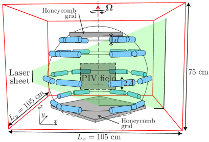
Figure 1: Experimental setup. 32 horizontal cylinders are tangent to an 80-cm-diameter virtual sphere horizontally centered in a water tank mounted on a rotating platform. The flow is bounded by two honeycomb grids at top and bottom (grey plates). The cylinders oscillate vertically at angular frequency $\omega_{0}$.

The entire apparatus is mounted on a 2-m-diameter platform rotating at a rate $\Omega$ ranging from $4.5$ to $18$ rpm around the vertical axis $z$. The cylinders oscillate at angular frequency $\omega_{0}=0.84\times 2\Omega$, generating self-similar inertial-wave beams Cortet2010 ; Machicoane2015 that spread as they propagate. The precise value $\omega_{0}/2\Omega=0.84$ is arbitrary and not crucial to our results. Nevertheless, it conveniently leads to most of the wave beams propagating toward the central region of the tank. The amplitude $A$ of oscillation of the cylinders ranges from a few millimeters to $25$ mm, leading to a forcing Reynolds number $270\leq Re=A\omega_{0}d/\nu\leq 3080$ for $\Omega=18$ rpm. The forcing Rossby number $A\omega_{0}/2\Omega d$ varies in the range $0.05\leq A\omega_{0}/2\Omega d\leq 0.52$ for $\Omega=18$ rpm (for $\Omega=4.5$ rpm, $250\leq Re\leq 710$ and $0.17\leq A\omega_{0}/2\Omega d\leq 0.48$). As the forcing amplitude increases, the overlapping wave beams generated by the 32 wavemakers produce a nearly statistically homogeneous flow in the central region (see movies of the velocity field in the Supplemental Material SM ).

A crucial modification to the previous version of the apparatus is the addition of two horizontal honeycomb grids (2.5 cm in height, 2.7 cm in mesh), one at the bottom of the tank and one at $59$ cm from the bottom (see Fig. 1). As shown in Ref. Brunet2020 , a single honeycomb grid efficiently damps geostrophic motion through enhanced turbulent drag on the rough grid topography, with little impact on wave dynamics. In the present study, we have included a second such grid to fully suppress spontaneous energy transfers to geostrophic modes, in a similar fashion to the numerical study of Le Reun et al. LeReun2017 . We have also upgraded the wave-driving mechanism to increase the maximum $Re$ by a factor of three.

Two components $(u_{x},u_{z})$ of the velocity field are measured in a vertical plane containing the center of the virtual sphere using a double-frame particle image velocimetry (PIV) system mounted on the rotating platform. The velocity fields have a spatial resolution of $1.93$ mm over an area of $\Delta x\times\Delta z=285\times 214$ mm² at the center of the virtual sphere (Fig. 1). For each experimental run, PIV acquisition covers $1250$ periods of the forcing in the statistically steady flow regime.

Temporal dynamics.— In the inset of Fig. 2, we show the temporal power spectral density $E(\omega^{*}=\omega/2\Omega)$ of the measured velocity field for $\Omega=18$ rpm and three values of $Re$. For the lowest forcing amplitude $Re=270$, the spectrum is dominated by a peak at normalized frequency $\omega_{0}^{*}=\omega_{0}/2\Omega=0.84$ corresponding to the waves forced by the wavemakers. The spectrum at $Re=310$ displays two additional subharmonic peaks, for two frequencies $\omega_{1}^{*}\simeq 0.29$ and $\omega_{2}^{*}\simeq 0.55$ in triadic resonance with the forcing frequency: $\omega_{1}^{*}+\omega_{2}^{*}=\omega_{0}^{*}$. These secondary peaks result from the TRI of the wave beams generated by the forcing Bordes2012 , i.e., the very first stage of nonlinear energy transfers between the base flow and other frequencies and spatial scales (TRI criteria for wave beams are discussed in Refs. Bourget2014 ; Fan2020 ). Finally, the spectrum at $Re=3080$ illustrates the regime of developed turbulence, where the flow has populated a continuous range of frequencies.

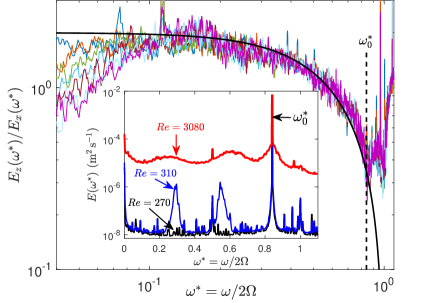
Figure 2: Ratio of the power spectral densities of the vertical and horizontal components of the velocity, for the experiments at $\Omega=18$ rpm and $Re=560,700,1060,1540,2020,2540$ and $3080$. The solid line $E_{z}/E_{x}=2(1-{\omega^{*}}^{2})/(1+{\omega^{*}}^{2})$ shows the behavior expected for an axisymmetric distribution of inertial waves. Inset: Power spectral density $E(\omega^{*})$ of the measured velocity field, for $\Omega=18$ rpm and three $Re$.

In the context of rotating turbulence, a natural question to ask is whether this energy is carried by inertial waves or geostrophic eddies. Indeed, in Brunet et al. Brunet2020 , we showed that the waves could spontaneously transfer energy to low-frequency geostrophic vortex modes. The absence of an energetic peak at $\omega=0$ in the spectra already indicates that such energy condensation into a geostrophic mode is suppressed by the honeycomb grids. An efficient way to test whether the spectral content corresponds to inertial waves consists in computing the ratio $E_{z}/E_{x}$ of the power spectral densities $E_{z}(\omega^{*})$ and $E_{x}(\omega^{*})$ of the horizontal and vertical velocity components, respectively. Indeed, for a single inertial wave, the ratio of the amplitudes of oscillation of the vertical and horizontal velocity components is directly set by the wave frequency $\omega^{*}$ Greenspan1968 . For an axisymmetric distribution of waves, this squared ratio becomes $E_{z}/E_{x}=2(1-{\omega^{*}}^{2})/(1+{\omega^{*}}^{2})$ Campagne2015 . In Fig. 2, we report the componential anisotropy factor $E_{z}/E_{x}$ for seven experiments at $\Omega=18$ rpm and $Re\geq 560$. The ratio $E_{z}/E_{x}$ closely follows the prediction for an axisymmetric distribution of inertial waves over a large range of frequencies $0.10<\omega^{*}<\omega_{0}^{*}=0.84$, which corresponds to typically $95\%$ of the total kinetic energy of the flow. This confirms that most of the energy is carried by inertial waves for rapid global rotation and high Reynolds number.

Generating such an ensemble of inertial waves is the number one pre-requisite to achieve weak turbulence in the laboratory. However, it is desirable to also investigate the validity of the more subtle assumptions of WTT: the large domain limit – to avoid purely discrete wave interactions – and the weak nonlinearity limit. To wit, we build on previous studies by Hasselmann et al. Hasselmann and Aubourg & Mordant Aubourg2016 and turn to the bicoherence spectrum $B(\omega_{1},\omega_{2})$ of the horizontal velocity component

$$B=\frac{|\langle\tilde{u}_{x}(x,z,\omega_{1})\tilde{u}_{x}(x,z,\omega_{2})\tilde{u}_{x}^{*}(x,z,\omega_{1}+\omega_{2})\rangle_{\bf x}|}{\sqrt{e(\omega_{1})e(\omega_{2})e(\omega_{1}+\omega_{2})}}\,,$$ (2)

where ^∗ denotes the complex conjugate, $\tilde{u}_{x}(x,z,\omega)$ is the temporal Fourier transform of the horizontal velocity, $\langle\,\rangle_{\bf x}$ is a spatial average over the measurement field and $e(\omega)=\langle|\tilde{u}_{x}(x,z,\omega)|^{2}\rangle_{\bf x}$. The bicoherence spectrum ranges from $B(\omega_{1},\omega_{2})=0$, when waves at frequencies $\omega_{1}$, $\omega_{2}$ and $\omega_{1}+\omega_{2}$ are uncorrelated, to $B(\omega_{1},\omega_{2})={\cal O}(1)$ when they are perfectly phase-correlated Aubourg2016 . For instance, in the canonical setup of the TRI, a base wave at frequency $\omega_{0}=\omega_{1}+\omega_{2}$ transfers energy to waves at frequencies $\omega_{1}$ and $\omega_{2}$, with a fixed relation between the phases of the three waves Bordes2012 . We thus expect the bicoherence to be ${\cal O}(1)$ for these values of $\omega_{1}$ and $\omega_{2}$. Such discrete resonances are also the signature of the so-called ‘discrete wave turbulence’ regime Kartashova2009 ; Lvov2010 ; Nazarenko2011 ; Brouzet2016 ; LeReun2017 ; LeReun2019 ; Davis2020 , where the temporal and/or spatial spectrum remains discrete. The framework of WTT departs from such discrete wave turbulence in two aspects: first, the large-domain limit, together with the nonlinear broadening of the resonances, leads to continuous spectra. Second, wave dispersion spontaneously induces a regime where the random-phase approximation holds Zakharov1992 ; Newell2011 ; Nazarenko2011 . More precisely, the derivation of the WTT stationary spectrum (1) proceeds through an expansion in the limit of low Rossby number $Ro$ (based on the injection scale and the rms velocity), recalled in the Supplemental Material (SM) SM . The dominant flow consists of inertial waves, described in terms of helical basis vectors Cambon89 ; Smith99 multiplied by slowly varying complex amplitudes $b_{s_{\bf i}}^{(0)}$, where ${\bf i}$ denotes the wave vector, the polarity $s_{\bf i}=\pm 1$ encodes the sign of the wave helicity, and the superscript $(0)$ denotes the lowest-order solution. The latter amplitudes have dimension of a velocity, and the phases of the various waves are uncorrelated. To lowest order, the numerator of $B$ consists of ensemble averages of triple products of the form $\langle b_{s_{\bf i}}^{(0)}b_{s_{\bf j}}^{(0)}b_{s_{\bf k}}^{(0)\,*}\rangle$, which vanish in the random-phase approximation according to Wick’s contraction rule Nazarenko2011 . One needs to consider the next order in the expansion, where smaller contributions $b_{s_{\bf i}}^{(1)}$ are forced by quadratic terms in $b_{s_{\bf i}}^{(0)}$. The expression of $b_{s_{\bf i}}^{(1)}$ is given in the SM SM , the simple order of magnitude estimate $b_{s_{\bf k}}^{(1)}\sim k\Omega^{-1}b_{s_{\bf i}}^{(0)\,*}b_{s_{\bf j}}^{(0)\,*}$ being sufficient for the present purpose (where the right-hand side really is a sum over many such terms for various wavenumbers ${\bf i}$ and ${\bf j}$ such that ${\bf i}+{\bf j}+{\bf k}={\bf 0}$). A nonzero contribution to the numerator of $B$ arises from terms of the form $\langle b_{s_{\bf i}}^{(0)}b_{s_{\bf j}}^{(0)}b_{s_{\bf k}}^{(1)\,*}\rangle\sim\langle b_{s_{\bf i}}^{(0)}b_{s_{\bf j}}^{(0)}b_{s_{\bf l}}^{(0)}b_{s_{\bf m}}^{(0)}\rangle k/\Omega\sim\langle|b_{s_{\bf i}}^{(0)}|^{2}\rangle\langle|b_{s_{\bf j}}^{(0)}|^{2}\rangle k/\Omega$, where we have used Wick’s contraction rule to transform the quartic term in wave amplitudes into a quadratic term in wave intensities. Denoting the generic wave intensity as $\langle|b_{s_{\bf i}}^{(0)}|^{2}\rangle$, we obtain an estimate for the bicoherence $B\sim\langle|b_{s_{\bf i}}^{(0)}|^{2}\rangle^{2}k/(\Omega\,\langle|b_{s_{\bf i}}^{(0)}|^{2}\rangle^{3/2})\sim\langle|b_{s_{\bf i}}^{(0)}|^{2}\rangle^{1/2}k/\Omega\sim Ro$. Instead of sharp isolated resonance peaks that stand out from a near-zero background, the bicoherence $B(\omega_{1},\omega_{2})$ is now a smooth function that takes low ${\cal O}(Ro)$ values.

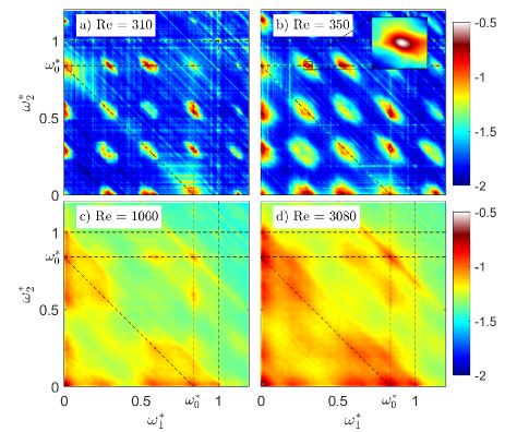
Figure 3: Logarithm of the bicoherence $B$ for $\Omega=18$ rpm and increasing values of $Re$.

In Fig. 3, we show the experimental bicoherence $B$ for four values of $Re$ at $\Omega=18$ rpm. For $Re=310$, slightly above the threshold of the TRI, the bicoherence map consists in an array of peaks localized at all coordinate values $(\omega_{1}^{*},\omega_{2}^{*})$ associated with two of the three energetic frequencies: $\omega^{*}\simeq 0.29$, $\omega^{*}\simeq 0.55$ and $\omega_{0}^{*}=0.84$. This is the signature of the TRI of the base waves, which induces a regime of discrete wave interactions, as described above. Further from the threshold of the first triadic instability, for $Re=350$, one notices the nonlinear broadening of the resonance peaks in the bicoherence map. At large distance from the TRI threshold, for $Re=3080$, the bicoherence has become a smooth function that takes low values ranging from $5\times 10^{-2}$ to $10^{-1}$, comparable to the Rossby number based on the rms velocity ($1.7$ cm/s) and the injection wavelength ($14$ cm inside the PIV plane), $Ro\simeq 3\times 10^{-2}$. The experimental bicoherence thus confirms the gradual transition from a discrete-wave-interaction regime to a proper weak turbulence regime as $Re$ increases. In the latter regime, the discreteness of the modes is smoothed out by the nonlinear broadening of the resonances, and both the temporal spectrum and the bicoherence become smooth functions. The bicoherence settles at a low value, of order $Ro$, compatible with a weakly nonlinear wave field that satisfies the random phase approximation.

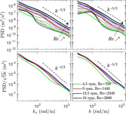
Figure 4: Spatial energy spectrum as a function of the horizontal wavenumber $k_{x}$ (left) and wavenumber $k=\sqrt{k_{x}^{2}+k_{z}^{2}}$ (right). Top panels: black thin lines correspond to $\Omega=18$ rpm and $Re$ increasing from $270$ to $3080$. Thick lines correspond to the highest Reynolds number for various rotation rates (see legend). Bottom panels: when rescaled by the spectral level predicted by WTT, the highest-$Re$ spectra at large $\Omega$ collapse onto a master curve. Dashed lines show the WTT power-law prediction.

Cascading states.— Having established that the turbulent flow is compatible with the assumptions of WTT at large $Re$, we turn to the spatial energy spectrum, with the goal of testing the predictions of WTT. We first compute the 2D spatial spectrum of the PIV velocity fields. In the left panels of Fig. 4, we integrate this 2D spectrum over the vertical wavenumber $k_{z}$ and show the resulting 1D spectrum as a function of $k_{x}$. In the right panels, we integrate the 2D spectrum over the angular direction instead, before plotting the resulting 1D spectrum as a function of the wavenumber $k=\sqrt{k_{x}^{2}+k_{z}^{2}}$. All the spectra in Fig. 4 are normalized in such a way that the integral of the spectrum over its variable ($\int{\rm PSD}(k_{x})\,dk_{x}$ or $\int{\rm PSD}(k)\,dk$) yields the space- and time-averaged kinetic energy inside the PIV domain. In the top panels, for weak driving amplitude, the spectra display a bump at a wavenumber corresponding to the injection wavelength. As the driving amplitude increases, the nonlinearities populate higher and higher wavenumbers in the spectrum, up to the point where a self-similar cascade develops: the high-$Re$ spectra then display a power-law behavior, with an exponent in close agreement with the prediction $-5/2$ of Eq. (1). This is clearly visible when the spectrum is shown as a function of $k_{x}$, for which the prediction is made, but also when the spectral content is shown as a function of $k$.

Beyond the prediction of the spectral exponent, WTT provides a prediction for the spectral level as a function of the rotation rate $\Omega$, the mean energy dissipation rate $\epsilon$, and the vertical wavelength $L_{\parallel}$ of the forced waves. In the highest-$Re$ experiments for the four values of $\Omega$ in Fig. 4, $L_{\parallel}$ is nearly constant and equal to $16$ cm. A direct measurement of $\epsilon$ is a notoriously difficult task, that requires well-resolved fully 3D velocity fields. The present PIV data are well-resolved but 2D. Assuming statistical axisymmetry, a proxy for $\epsilon$ can be obtained from the velocity gradients accessible in the measurement plane:

$$\epsilon\simeq\nu\langle 2\left(\partial_{x}u_{x}\right)^{2}+2\left(\partial_{x}u_{z}\right)^{2}+2\left(\partial_{z}u_{x}\right)^{2}+\left(\partial_{z}u_{z}\right)^{2}\rangle_{{\bf x},t},$$

where $\langle\,\rangle_{{\bf x},t}$ is a spatial and temporal average. Using this proxy, we plot in Fig. 4 the rescaled spectra ${\rm PSD}/\sqrt{\Omega\epsilon}$, for the highest Reynolds number achieved at each rotation rate. This representation leads to a collapse of the high-$\Omega$ spectra onto a master curve that follows the $k^{-5/2}$ power-law dependence. The experimental data thus validate the predictions of WTT, both for the spectral level and the spectral exponent, provided molecular dissipation is negligible (high $Re$) and the wave turbulence is weakly nonlinear (high $\Omega$, low $Ro$).

Discussion.— The present experimental apparatus allows us to generate a turbulent flow that consists of weakly interacting inertial waves in a large fluid domain. As the forcing increases, the system transitions from a regime of discrete wave interactions to a regime that displays continuous temporal spectra and bicoherence maps, in line with WTT. At high Reynolds number and low Rossby number, the resulting spatial spectrum exhibits the scaling properties predicted by WTT, both in terms of spectral slope and spectral level. Such a laboratory realization of weak turbulence in a 3D fluid system could open an experimental avenue for studies that gradually incorporate the additional complexities of natural flows. Among the many exciting directions for future research, one could add density stratification to characterize the turbulent mixing induced by inertia-gravity waves in the weak-turbulence regime Lvov2001 , and one could progressively relax the damping of the geostrophic flow to characterize its impact on the wave-turbulent dynamics. Following Scott Scott2014 , it may be that the large-scale geostrophic flow sweeps the wave phases and challenges a precise characterization of the wave dynamics, but that the small-scale cascading dynamics remains largely unaffected. The consequence would be that WTT remains a valuable tool to charaterize small-scale dissipation and to develop subgrid-scale parameterizations in that context.

- (1) V.E. Zakharov, V.S. L’vov, and G. Falkovich, Kolmogorov Spectra of Turbulence (Springer, Berlin, 1992).
- (2) A.C. Newell and B. Rumpf, Wave Turbulence, Annu. Rev. Fluid Mech. 43, 59 (2011).
- (3) S. Nazarenko, Wave Turbulence (Springer, Berlin, 2011).
- (4) J. Pedlosky, Geophysical Fluid Dynamics (Springer-Verlag, New York, 1987).
- (5) P.A. Davidson, Turbulence in Rotating, Stratified and Electrically Conducting Fluids (Cambridge University Press, Cambridge, 2013).
- (6) M.C. Gregg, E.A. D’Asaro, J.J Riley, and E. Kunze, Mixing Efficiency in the Ocean, Annu. Rev. Mar. Sci. 10, 443 (2018).
- (7) E. Falcon, C. Laroche, and S. Fauve, Observation of gravity-capillary wave turbulence, Phys. Rev. Lett. 98, 094503 (2007).
- (8) P. Clark di Leoni, P.J. Cobelli, and P.D. Mininni, Wave turbulence in shallow water models, Phys. Rev. E 89, 063025 (2014).
- (9) Q. Aubourg and N. Mordant, Investigation of resonances in gravity-capillary wave turbulence, Phys. Rev. Fluids 1, 023701 (2016).
- (10) M. Berhanu, E. Falcon, G. Michel, C. Gissinger, and S. Fauve, Capillary wave turbulence experiments in microgravity, Europhys. Lett. 128, 34001 (2019).
- (11) P. Cobelli, P. Petitjeans, A. Maurel, V. Pagneux, and N. Mordant, Space-Time Resolved Wave Turbulence in a Vibrating Plate, Phys. Rev. Lett. 103, 204301 (2009).
- (12) T. Humbert, O. Cadot, G. Düring, C. Josserand, S. Rica, and C. Touzé, Wave turbulence in vibrating plates: The effect of damping, Europhys. Lett. 102, 30002 (2013).
- (13) B. Miquel, A. Alexakis, C. Josserand, and N. Mordant, Transition from Wave Turbulence to Dynamical Crumpling in Vibrated Elastic Plates, Phys. Rev. Lett. 111, 054302 (2013).
- (14) H. Greenspan, The Theory of Rotating Fluids (Cambridge University Press, Cambridge, 1968).
- (15) S. Galtier, Weak inertial-wave turbulence theory, Phys. Rev. E 68, 015301 (2003).
- (16) S.V. Nazarenko and A.A. Schekochihin, Critical balance in magnetohydrodynamic, rotating and stratified turbulence: towards a universal scaling conjecture, J. Fluid Mech. 677, 134 (2011).
- (17) S. Galtier and V. David, Inertial/kinetic-Alfvén wave turbulence: A twin problem in the limit of local interactions, Phys. Rev. Fluids 5, 044603 (2020).
- (18) E.J. Hopfinger, F.K. Browand, and Y. Gagne, Turbulence and waves in a rotating tank, J. Fluid Mech. 125, 505 (1982).
- (19) E. Yarom, Y. Vardi, and E. Sharon, Experimental quantification of inverse energy cascade in deep rotating turbulence, Phys. Fluids 25, 085105 (2013).
- (20) A. Campagne, B. Gallet, F. Moisy, and P.-P. Cortet, Disentangling inertial waves from eddy turbulence in a forced rotating-turbulence experiment, Phys. Rev. E 91, 043016 (2015).
- (21) A. Sen, P.D. Mininni, D. Rosenberg, and A. Pouquet, Anisotropy and nonuniversality in scaling laws of the large-scale energy spectrum in rotating turbulence, Phys. Rev. E 86, 036319 (2012).
- (22) P. Clark di Leoni, P.J. Cobelli, P.D. Mininni, P. Dmitruk, and W.H. Matthaeus, Quantification of the strength of inertial waves in a rotating turbulent flow, Phys. Fluids 26, 035106 (2014).
- (23) E. Deusebio, G. Boffetta, E. Lindborg, and S. Musacchio, Dimensional transition in rotating turbulence, Phys. Rev. E 90, 023005 (2014).
- (24) L. Jacquin, O. Leuchter, C. Cambon, and J. Mathieu, Homogeneous turbulence in the presence of rotation, J. Fluid Mech. 220, 1 (1990).
- (25) P.J. Staplehurst, P.A. Davidson, and S.B. Dalziel, Structure formation in homogeneous freely decaying rotating turbulence, J. Fluid Mech. 598, 81 (2008).
- (26) C. Lamriben, P.-P. Cortet, and F. Moisy, Direct Measurements of Anisotropic Energy Transfers in a Rotating Turbulence Experiment, Phys. Rev. Lett. 107, 024503 (2011).
- (27) A. Campagne, N. Machicoane, B. Gallet, P.-P. Cortet, and F. Moisy, Turbulent drag in a rotating frame, J. Fluid Mech. 794, R5 (2016).
- (28) C.N. Baroud, B.B. Plapp, H.L. Swinney, and Z.S. She, Scaling in three-dimensional and quasi-two-dimensional rotating turbulent flows, Phys. Fluids 15, 2091 (2003).
- (29) T. Le Reun, B. Favier, and M. Le Bars, Experimental study of the nonlinear saturation of the elliptical instability: inertial wave turbulence versus geostrophic turbulence, J. Fluid Mech. 879, 296 (2019).
- (30) M. Brunet, B. Gallet and P.-P. Cortet, Shortcut to Geostrophy in Wave-Driven Rotating Turbulence: The Quartetic Instability, Phys. Rev. Lett. 124, 124501 (2020).
- (31) E. Yarom and E. Sharon, Experimental observation of steady inertial wave turbulence in deep rotating flows, Nature Physics 10, 510 (2014).
- (32) E. Yarom, A. Salhov, and E. Sharon, Experimental quantification of nonlinear time scales in inertial wave rotating turbulence, Phys. Rev. Fluids 2, 122601(R) (2017).
- (33) T. Le Reun, B. Favier, A.J. Barker, and M. Le Bars, Inertial Wave Turbulence Driven by Elliptical Instability, Phys. Rev. Lett. 119, 034502 (2017).
- (34) C. Connaughton, S. Nazarenko, A.C. Newell, Dimensional analysis, Weak turbulence approximation, Incomplete self-similarity, Physica D 184, 86 (2003).
- (35) P.-P. Cortet, C. Lamriben, and F. Moisy, Viscous spreading of an inertial wave beam in a rotating fluid, Phys. Fluids 22, 086603 (2010).
- (36) N. Machicoane, P.-P. Cortet, B. Voisin, and F. Moisy, Influence of the multipole order of the source on the decay of an inertial wave beam in a rotating fluid, Phys. Fluids 27, 066602 (2015).
- (37) See Supplemental Material at XXXX for movies of the velocity field and details about the decomposition onto the helical basis vectors.
- (38) G. Bordes, F. Moisy, T. Dauxois, and P.-P. Cortet, Experimental evidence of a triadic resonance of plane inertial waves in a rotating fluid, Phys. Fluids 24, 014105 (2012).
- (39) B. Bourget, H. Scolan, T. Dauxois, M. Le Bars, P. Odier, and S. Joubaud, Finite-size effects in parametric subharmonic instability, J. Fluid Mech. 759, 739 (2014).
- (40) Boyu Fan and T.R. Akylas, Finite-amplitude instabilities of thin internal wave beams: experiments and theory, J. Fluid Mech. 904, A16 (2020).
- (41) K. Hasselmann, W. Munk, and G. MacDonald, Bispectra of ocean waves, in Time Series Analysis, ed. M. Rosenblatt, 125-139, John Wiley (1963).
- (42) E. Kartashova, Discrete wave turbulence, Europhys. Lett. 87, 44001 (2009).
- (43) V.S. L’vov and S. Nazarenko, Discrete and mesoscopic regimes of finite-size wave turbulence, Phys. Rev. E 82, 056322 (2010).
- (44) C. Brouzet, E. V. Ermanyuk, S. Joubaud, I. Sibgatullin, and T. Dauxois, Energy cascade in internal-wave attractors, Europhys. Lett. 113, 4 (2016).
- (45) G. Davis, T. Jamin, J. Deleuze, S. Joubaud, and T. Dauxois, Succession of Resonances to Achieve Internal Wave Turbulence, Phys. Rev. Lett. 124, 204502 (2020).
- (46) C. Cambon and L. Jacquin, Spectral approach to non-isotropic turbulence subjected to rotation, J. Fluid Mech. 202, 295 (1989).
- (47) L.M. Smith and F. Waleffe, Transfer of energy to two-dimensional large scales in forced, rotating three-dimensional turbulence, Phys. Fluids 11, 1608 (1999).
- (48) J.F. Scott, Wave turbulence in a rotating channel, J. Fluid Mech. 741, 316 (2014).
- (49) Y.V. Lvov and E.G. Tabak, Hamiltonian Formalism and the Garrett-Munk Spectrum of Internal Waves in the Ocean, Phys. Rev. Lett. 87, 168501 (2001).