The ground state of polaron in an ultracold dipolar Fermi gas

Abstract

An impurity atom immersed in an ultracold atomic Fermi gas can form a quasiparticle, so-called Fermi polaron, due to impurity-fermion interaction. We consider a three-dimensional homogeneous dipolar Fermi gas as a medium, where the interatomic dipole-dipole interaction (DDI) makes the Fermi surface deformed into a spheroidal shape, and, using a Chevy-type variational method, investigate the ground-state properties of the Fermi polaron: the effective mass, the momentum distribution of a particle-hole (p-h) excitation, the drag parameter, and the medium density modification around the impurity. These quantities are shown to exhibit spatial anisotropies in such a way as to reflect the momentum anisotropy of the background dipolar Fermi gas. We have also given numerical results for the polaron properties at the unitarity limit of the impurity-fermion interaction in the case in which the impurity and fermion masses are equal. It has been found that the transverse effective mass and the transverse momentum drag parameter of the polaron both tend to decrease by $\sim 10\%$ when the DDI strength is raised from $0$ up to around its critical value, while the longitudinal ones exhibit a very weak dependence on the DDI.

I Introduction

The concept of a polaron was originally suggested by Landau and Pekar to describe the electron conduction in ionic crystal lattices Zh.Eksp.Teor.Fiz16.341(1946) ; Zh.Eksp.Teor.Fiz.18.419(1948) : When slowly moving electrons in a lattice polarize ions around them, the electron dressed in the local polarization of ions behaves as a quasiparticle, i.e., the polaron. Nowadays, the polaron concept is used in more general cases in which impurities in a degenerate medium are accompanied by medium excitations due to impurity-medium interactions.

In the past decade, ultracold atoms have offered new opportunities both in theoretical and experimental studies of the polaron problem. Typically, an impurity atom interacts with atoms in the medium of an ultracold Fermi/Bose gas and forms a quasiparticle called Fermi/Bose polaron. In fact, these kinds of polarons have been observed in experiments that utilize radio-frequency response techniques (see Refs. PhysRevLett.102.230402 ; 2012Natur.485..615K ; Scazza_2017 for Fermi polarons and Refs. 2012PhRvA..85b3623C ; 2013PhRvL.111g0401S ; 2016PhRvL.117e5301H ; 2016PhRvL.117e5302J for Bose polarons). One of the intriguing features of these ultracold atomic polarons is experimental controllability of the system characteristics, such as particle statistics, interaction strength, and dimensionality, which would help to verify various theoretical studies of the polaron problem. For instance, because of dominance of the low-energy scattering processes in ultracold dilute medium, not only are the atomic interactions characterized by a few scattering parameters, namely, the scattering lengths and the effective ranges, but also their strengths are tunable by external field RevModPhys.82.1225 . Another feature, which is more characteristic of polarons themselves, is the dependence of the polaron properties on the Fermi/Bose particle statistics of the medium. In the medium of a Bose gas, the excitations caused by the impurity atom are Bogoliubov phonons on top of the Bose-Einstein condensate (BEC) 2015PhRvA..92c3612A ; 2013PhRvA..88e3632R ; 2016PhRvL.117k3002S , while in the medium of a degenerate Fermi gas, various kinds of particle-hole-pair excitations near the Fermi surface behave as effective degrees of freedom and interact with the impurity PhysRevLett.97.200403 ; PhysRevLett.98.180402 ; 2012PhRvA..85c3631B ; Trefzger_2013 . Particularly in a strong coupling regime of the impurity-medium interaction, the impurity and the excitations can constitute few-body bound states, e.g., dimer molecules, Efimov-like states, tetramers, and so on PhysRevA.80.053605 ; 2015PhRvA..92c3612A ; 2015PhRvL.115l5302L ; 2016PhRvL.117k3002S ; 2014RPPh…77c4401M .

In the present study, instead of treating such possible few-body correlations beyond the polaron picture, we focus on the medium effect on quasiparticle properties of a single polaron by taking a dipolar Fermi gas as the surrounding medium, whose salient features are the anisotropic and long-range nature of the dipole-dipole interaction (DDI). In the preceding theoretical studies based on a variational method within the Hartree-Fock (HF) approximation, it has been shown that the DDI causes a Fermi surface deformation (FSD) in the ground state of a spin polarized dipolar Fermi gas PhysRevA.77.061603 ; Sogo_2009 . Such an exotic state, however, may not be robust for strong DDI strengths. In fact, it has been predicted from theoretical studies of density fluctuations in dipolar Fermi gases Chan_2010 ; Ronen_2010 ; Kestner_2010 that above a critical strength, the FSD becomes unstable with respect to growth of density waves with an infinitesimal wave vector in the direction perpendicular to the dipoles. Such instability of a dipolar Fermi gas has also been reported from a thermodynamic point of view based on the energy functional approach Sogo_2009 ; PhysRevA.84.053603 ; PhysRevA.91.023612 . In experiments, ultracold dipolar Fermi gases have been realized for highly magnetic atoms and for polar molecules having large magnetic or electric dipole moments Lu_2012 ; PhysRevLett.112.010404 ; Naylor_2015 ; DeMarco_2019 , and remarkably Aikawa et al. aikawa2014observation has observed the FSD in a degenerate dipolar Fermi gas of Er atoms.

Inspired by such theoretical and experimental progress, in this paper we consider a single nondipolar atomic impurity moving in a three-dimensional homogeneous dipolar Fermi gas at zero temperature and then examine how its quasiparticle properties such as the effective mass and the particle-hole excitations around the impurity depend on the direction and strength of the DDI via the resulting FSD. By observing the medium density distribution around the impurity, furthermore, we briefly discuss a possible instability of the system toward a density collapse, which can be triggered by impurities through the attraction with the dipolar gas that is already susceptible to density fluctuations in the presence of the DDI. In the present calculations, we take the unitarity limit in the impurity-medium interaction to compare our results for the spatially anisotropic medium with the existing numerical data obtained for the spatially isotropic medium at the unitarity limitPhysRevA.74.063628 ; PhysRevLett.103.170402 . It should be noted that the polaron problem in a dipolar Bose gas has been studied in Refs. PhysRevA.89.023612 ; 2019JPhB…52a5004A , in which effects of the Bogoliubov phonons in a dipolar BEC on the polaron dispersion relation and spectrum intensity have been clarified.

In Sec. II, we introduce the formalism to describe a single atomic impurity in a dipolar Fermi gas and then give an effective Hamiltonian of the system by using the single particle energy of the dipolar Fermi gas obtained from the HF calculation. To obtain the ground state wave function, we employ the variational method developed by Chevy PhysRevA.74.063628 in such a way as to include a single pair of particle-hole (p-h) excitations near the deformed Fermi surface. In Sec. III, we show the numerical results for the polaron energy, the transverse and longitudinal effective masses, the drag parameter that characterizes the momentum distribution of p-h excitations, and the medium density modification, together with discussions on these results. Section IV is devoted to summary and outlook. In this paper, we use units in which $\hbar=1$.

II Formalism

In this section, we start with the full Hamiltonian for the system of a single impurity in a uniform dipolar Fermi gas of single atomic species, and implement the Lee-low-Pines (LLP) transformation Phys.Rev.90.297 to obtain the Hamiltonian written in terms only of the dipolar fermions. We then apply the HF approximation to the dipolar Fermi gas, and obtain an effective Hamiltonian, from which we calculate various properties of the Fermi polaron.

II.1 Full Hamiltonian

First we consider a homogeneous gas of single-component dipolar fermions at zero temperature, whose Hamiltonian is given by

$$H_{d} =\int_{\bm{r}}\psi^{\dagger}(\bm{r})\frac{-\nabla^{2}}{2m}\psi(\bm{r})+\frac{1}{2}\int_{r,r^{\prime}}\psi^{\dagger}(\bm{r}^{\prime})\psi^{\dagger}(\bm{r})V_{dd}(\bm{r}-\bm{r}^{\prime})\psi(\bm{r})\psi(\bm{r}^{\prime}),$$ (1)

where the field operator $\psi(\bm{r})$ is for a fermion with the mass $m$, and $\int_{r}$ is the abbreviation of the integration over volume $V$, $\int_{V}d^{3}r$. With the strength of the dipole moment $d=|{\bm{d}}|$, the DDI $V_{dd}(\bm{r})$ is given by

$$V_{dd}(\bm{r}) =\frac{d^{2}}{r^{3}}\left(1-3\frac{z^{2}}{r^{2}}\right),$$ (2)

where the dipole moments are assumed to be polarized along the z-axis. The Fourier transform of $V_{dd}(\bm{r})$ becomes

$$\tilde{V}_{dd}(\bm{q})=\int_{r}V_{dd}(\bm{r})e^{-i{\bm{q}}\cdot{\bm{r}}}=\frac{4\pi}{3}d^{2}\left(3\cos^{2}\theta_{\bm{q}}-1\right),$$ (3)

where $\theta_{\bm{q}}$ is the angle between the momentum transfer ${\bm{q}}$ and the dipole moment ${\bm{d}}$. Note that in this Hamiltonian, there is no contact interaction between two fermions in the polarized (single component) medium. Even in the presence of such contact interaction, the Pauli exclusion principle would allow us to ignore the resultant low-energy scattering.

Now let us introduce a single non-dipolar impurity of the mass $M$, which interacts with the dipolar medium fermions with a coupling constant $g$. Then the full Hamiltonian of the impurity and the medium dipolar Fermi gas is given by

$$H(\bm{x}) =H_{d}-\frac{\nabla_{x}^{2}}{2M}+g\int_{r}\psi^{\dagger}(\bm{r})\psi(\bm{r})\delta(\bm{r}-\bm{x})$$

$$=\sum_{\bm{q}}\frac{q^{2}}{2m}a_{\bm{q}}^{\dagger}a_{\bm{q}}+\frac{1}{2}\sum_{\bm{q},\bm{q}^{\prime},\bm{s}}a_{\bm{q}^{\prime}-\bm{s}}^{\dagger}a_{\bm{q}+\bm{s}}^{\dagger}a_{\bm{q}}a_{\bm{q}^{\prime}}\tilde{V}_{dd}(\bm{s})$$

$$\qquad-\frac{\nabla_{x}^{2}}{2M}+g\sum_{\bm{q},\bm{q}^{\prime}}a_{\bm{q}}^{\dagger}a_{\bm{q}^{\prime}}e^{-i(\bm{q}-\bm{q}^{\prime})\cdot\bm{x}}.$$ (4)

Here we have used the first quantization for the impurity in the coordinate representation $\bm{x}$, and expanded the field operator of fermions as $\psi(\bm{r})=\frac{1}{\sqrt{V}}\sum_{\bm{q}}e^{i\bm{q}\cdot\bm{r}}a_{\bm{q}}$, where the creation and annihilation operators $a_{\bm{q}}^{\dagger}$ and $a_{\bm{q}}$ satisfy the canonical commutation relation:

$$\left\{a_{\bm{q}},a_{\bm{q}^{\prime}}^{\dagger}\right\}=\delta_{\bm{q},\bm{q}^{\prime}}.$$ (5)

It should be noted that the coupling constant $g$ is related to the $s$-wave scattering length $a$ via the Lippmann-Schwinger equation at the low energy limit:

$$g^{-1} =\frac{m_{r}}{2\pi a}-\sum_{\bm{q}}\frac{2m_{r}}{q^{2}},$$ (6)

where the reduced mass $m_{r}$ is defined in $m_{r}^{-1}=m^{-1}+M^{-1}$.

II.2 LLP transformation

Now we apply the Lee-Low-Pines theoryPhys.Rev.90.297 to the Hamiltonian defined in the previous subsection. We define the operator $S(\bm{x})$ with the momentum operator of medium fermions $\hat{\bm{P}}$:

$$S(\bm{x})=e^{i\bm{x}\cdot\hat{\bm{P}}}\qquad\mbox{where}\qquad\hat{\bm{P}}=\sum_{\bm{q}}\bm{q}a_{\bm{q}}^{\dagger}a_{\bm{q}}.$$ (7)

This operator generates the LLP transformation for the annihilation operator $a_{\bm{q}}$ as

$$S(\bm{x})a_{\bm{q}}S^{-1}(\bm{x})=a_{\bm{q}}e^{-i\bm{q}\cdot\bm{x}}.$$ (8)

It should be noted that it transforms fermions to the co-moving frame of the impurity in which the impurity keeps staying at the origin. The Hamiltonian is then transformed as

$$S(\bm{x})H(\bm{x})S(\bm{x})^{-1} =\sum_{\bm{q}}\frac{q^{2}}{2m}a_{\bm{q}}^{\dagger}a_{\bm{q}}+\frac{1}{2}\sum_{\bm{q},\bm{q}^{\prime},\bm{s}}a_{\bm{q}^{\prime}-\bm{s}}^{\dagger}a_{\bm{q}+\bm{s}}^{\dagger}a_{\bm{q}}a_{\bm{q}^{\prime}}\tilde{V}_{dd}(\bm{s})$$

$$\qquad+\frac{\left(-i\bm{\nabla}_{x}-\hat{\bm{P}}\right)^{2}}{2M}+g\sum_{\bm{q},\bm{q}^{\prime}}a_{\bm{q}}^{\dagger}a_{\bm{q}^{\prime}},$$ (9)

which in turn satisfies the commutation relation:

$$\left[S(\bm{x})H(\bm{x})S(\bm{x})^{-1},-i\bm{\nabla}_{x}\right]=0.$$ (10)

This relation implies that the derivative operator $-i\bm{\nabla}_{x}$ can be replaced with a $c$-number momentum, i.e., $-i\bm{\nabla}_{x}=\bm{P}$. This impurity momentum $\bm{P}$ corresponds to the total momentum of the transformed system (or a polaron) via $S(-i\bm{\nabla}_{x}+\hat{\bm{P}})S^{-1}=-i\bm{\nabla}_{x}$. It should be noted that $SHS^{-1}$ and $H$ are of unitary equivalence by the $S$ transformation, and hence the dependence of the impurity coordinate $\bm{x}$ in the original wave function can always be recovered by the inverse transformation.

II.3 Mean-field description of dipolar Fermi gas

It has been shown that a spin polarized dipolar Fermi gas takes on a deformed Fermi surface due to the exchange contribution of the DDI PhysRevA.77.061603 . In the mean-field approximation, the single-particle energy $\varepsilon_{\bm{q}}$ of fermions can be obtained from a self-consistent HF equation as

$$\varepsilon_{\bm{q}}=\frac{q^{2}}{2m}-\sum_{\bm{q}^{\prime}}\tilde{V}_{dd}(\bm{q}-\bm{q}^{\prime})n_{\bm{q}^{\prime}},$$ (11)

where the second term is the exchange contribution with the Fermi-Dirac distribution function given by $n_{\bm{q}}=\theta(\epsilon_{F}-\varepsilon_{\bm{q}})$ at zero temperature; $\epsilon_{F}$ is the Fermi energy. The direct contribution vanishes due to the symmetry in the momentum space. In Ref. Ronen_2010 , it is shown that the Fermi surface determined from numerical calculations of the self-consistent single-particle energy can be well described by a spheroidal form:

$$n_{\bm{q}}=\theta\left(k_{F}^{2}-\frac{1}{\beta}[q_{x}^{2}+q_{y}^{2}]-\beta^{2}q_{z}^{2}\right),$$ (12)

where $k_{F}$ is the Fermi momentum for non-interacting fermions. The deformation parameter $\beta$ is in general less than one ($\beta<1$) due to the attractive nature of the exchange energy, leading to a prolate shape of the Fermi surface. For weak DDI strengths, $\beta$ has been calculated in Ref. Ronen_2010 as

$$\beta=1-\frac{2md^{2}k_{F}}{9\pi}.$$ (13)

In this study, instead of solving the self-consistent HF equation (11) numerically, we use a model single-particle energy that reproduces the deformed Fermi surface:

$$\varepsilon_{\bm{q}}=\varepsilon_{0}+\frac{1}{2m_{t}(q)}(q_{x}^{2}+q_{y}^{2})+\frac{1}{2m_{z}(q)}q_{z}^{2},$$ (14)

where $\varepsilon_{0}$ is an energy shift. The momentum-dependent effective masses, $m_{z}(q)$ and $m_{t}(q)$, are given by

$$\frac{m_{z}(q)}{m} =\left(\frac{1}{\lambda^{2}\beta^{2}}-1\right)e^{-\frac{q^{2}}{k_{c}^{2}}}+1,$$ (15)

$$\frac{m_{t}(q)}{m} =\left(\frac{\beta}{\lambda^{2}}-1\right)e^{-\frac{q^{2}}{k_{c}^{2}}}+1,$$ (16)

where $q=|\bm{q}|$, and $\lambda$ denotes the curvature of the single particle energy. The parameters $\beta$, $\lambda$, and $k_{c}$ are determined from detailed calculations of the ground state properties based on such a variational method as given in Refs. Sogo_2009 ; Yamaguchi_2010 ; numerical values of these parameters depend on a dimensionless DDI coupling constant defined as

$$C_{dd}=md^{2}n_{f}^{1/3},$$ (17)

where

$$n_{f}=\frac{k_{F}^{3}}{6\pi^{2}}$$ (18)

is the density of the dipolar Fermi gas. See TABLE 1 for the values of $\beta$ and $\lambda^{2}$ at various $C_{dd}$’s, where the value of $k_{c}$ has been determined to be $2.5k_{F}$ independently of the value of $C_{dd}$ in such a way that the model single particle energy (14) is consistent with the HF calculations.

$C_{dd}$	$0$	$0.25$	$0.5$	$0.75$	$1.0$	$1.25$	$1.5$
$\beta$	$1.0000$	$0.9340$	$0.8747$	$0.8224$	$0.7769$	$0.7374$	$0.7032$
$\lambda^{2}$	$1.0000$	$1.0048$	$1.0188$	$1.0411$	$1.0702$	$1.1046$	$1.1429$

Table 1: The values of $\beta$ and $\lambda^{2}$

The model single-particle energy (14), together with the momentum-dependent effective masses (15) and (16), recovers the free-particle spectrum for large $q$; such asymptotic behavior is guaranteed in the self-consistent single particle energy (11). Fig. 1 depicts the behaviors of the model single-particle energies for $C_{dd}=1.0$, together with numerical results from the self-consistent HF equation; they are found to be almost on the top of each other. Details of how we obtain the model single-particle energy and momentum-dependent effective masses on the basis of the variational method are given in Appendix A.

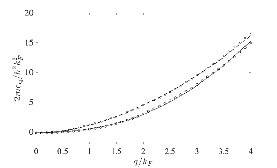
Figure 1: Model single-particle energies $\epsilon(0,0,q)$ (solid line) and $\epsilon(q,0,0)$ (dashed line) as plotted in the presence of the DDI ($C_{dd}=1.0$) as a function of $q$. In this calculation, the parameters are fixed as $\beta=0.7769$, $\lambda^{2}=1.0702$, and $k_{c}=2.5k_{F}$. The corresponding single-particle energies are also derived from numerical calculations in the HF approximation (circles and crosses).

II.4 Effective Hamiltonian

Introduction of the impurity in the medium Fermi gas brings about the particle-hole (p-h) excitations near the deformed Fermi surface. Now we assume that the medium modification can be calculated in perturbation theory, while basic properties of the medium dipolar Fermi gas are essentially unchanged. Then we can construct an effective Hamiltonian from Eq. (9) in terms only of medium fermions as

$$S(\bm{x})H(\bm{x})S(\bm{x})^{-1}\quad\rightarrow\quad H_{\mathrm{e}ff}(\bm{P})=\sum_{\bm{q}}\varepsilon_{\bm{q}}a_{\bm{q}}^{\dagger}a_{\bm{q}}+\frac{(\bm{P}-\hat{\bm{P}})^{2}}{2M}+g\sum_{\bm{q},\bm{q}^{\prime}}a_{\bm{q}}^{\dagger}a_{\bm{q}^{\prime}},$$ (19)

where we have replaced the impurity’s momentum operator $-i\bm{\nabla}_{x}$ by the total momentum of the system $\bm{P}$. In the above effective Hamiltonian, no dynamical degrees of freedom of the impurity exist PhysRevA.96.033627 . We can thus find the ground state of the system from the dipolar fermion Hamiltonian (19), which includes a deformed single-particle energy term (the first term) and the self-interaction terms (the second and the third terms).

III Polaron properties

In this section, using a variational method, we obtain the ground-state wave function for the polaron with the momentum $\bm{P}$, with which numerical results are shown for the rest energy (binding energy), the effective masses, the momentum drag parameters, and density fluctuations around the impurity. Discussions are finally given on these results.

III.1 Single particle-hole pair approximation

By following a useful approach to the spin imbalanced Fermi gas problem PhysRevA.74.063628 ; PhysRevLett.98.180402 , let us set up a variational state $|\Psi\rangle$ that includes excitations of a single p-h pair near the deformed Fermi surface:

$$|\Psi\rangle=F_{0}|fs\rangle+\sum_{k>,p<}F_{\bm{k},\bm{p}}a_{\bm{k}}^{\dagger}a_{\bm{p}}|fs\rangle,$$ (20)

where $|fs\rangle$ is the Fermi degenerate state that has fermions occupied up to the deformed Fermi surface, $k>$ ($p<$) denotes the summation over momenta above (below) the Fermi surface, and $F_{0}$ and $F_{\bm{k},\bm{p}}$ are variational parameters that satisfy the normalization condition:

$$|F_{0}|^{2}+\sum_{k>,p<}|F_{\bm{k},\bm{p}}|^{2}=1.$$ (21)

It should be noted that in the absence of the DDI, the above simple variational ansatz (20) works for the description of polaronic properties even in the strongly attractive regime close to the unitarity limit PhysRevB.77.020408 ; 2014RPPh…77c4401M ; 2018NJPh…20g3048T .

The expectation value of the effective Hamiltonian (20) is represented by

$$\langle H_{\mathrm{e}ff}(\bm{P})\rangle =\sum_{\bm{q}}\varepsilon_{\bm{q}}\langle a_{\bm{q}}^{\dagger}a_{\bm{q}}\rangle+\frac{\left\langle(\bm{P}-\hat{\bm{P}})^{2}\right\rangle}{2M}+g\sum_{\bm{q},\bm{q}^{\prime}}\langle a_{\bm{q}}^{\dagger}a_{\bm{q}^{\prime}}\rangle,$$ (22)

where $\langle O\rangle$ is the expectation value of the operator $O$ with respect to the state $|\Psi\rangle$: $\langle O\rangle=\langle\Psi|O|\Psi\rangle$. Substitution of the state (20) leads to the explicit representation of each term in the right side of Eq. (22) as

$$\sum_{\bm{q}}\varepsilon_{\bm{q}}\langle a_{\bm{q}}^{\dagger}a_{\bm{q}}\rangle =\sum_{q<}\varepsilon_{\bm{q}}\biggr{(}|F_{0}|^{2}+\sum_{k>,p<}|F_{\bm{k},\bm{p}}|^{2}\biggr{)}+\sum_{q>,p<}\varepsilon_{\bm{q}}|F_{\bm{q},\bm{p}}|^{2}-\sum_{k>,q<}\varepsilon_{\bm{q}}|F_{\bm{k},\bm{q}}|^{2},$$ (23)

$$\left\langle(\bm{P}-\hat{\bm{P}})^{2}\right\rangle =P^{2}|F_{0}|^{2}+\sum_{k>,p<}|F_{\bm{k},\bm{p}}|^{2}[P^{2}-2\bm{P}\cdot(\bm{k}-\bm{p})+(\bm{k}-\bm{p})^{2}],$$ (24)

$$\sum_{\bm{q},\bm{q}^{\prime}}\langle a_{\bm{q}}^{\dagger}a_{\bm{q}^{\prime}}\rangle =\sum_{q<}\left(|F_{0}|^{2}+\sum_{k>,p<}|F_{\bm{k},\bm{p}}|^{2}\right)$$

$$+\sum_{k>,p<}(F_{0}F_{\bm{k},\bm{p}}^{*}+F_{0}^{*}F_{\bm{k},\bm{p}})+\sum_{q>,q^{\prime}>,p<}F_{\bm{q},\bm{p}}^{*}F_{\bm{q}^{\prime},\bm{p}}-\sum_{k>,q<,q^{\prime}<}F_{\bm{k},\bm{q}}^{*}F_{\bm{k},\bm{q}^{\prime}}.$$ (25)

III.2 p-h momentum distribution and polaron energy

We impose the normalization condition (21) on the variational state by introducing a Lagrange multiplier $\mu$ that turns out to be the energy of the system with the momentum $\bm{P}$. Up to the contribution of the energy of the background dipolar fermions, $\mu$ reads

$$\mu=E(\bm{P})+\sum_{q<}\varepsilon_{\bm{q}},$$ (26)

where $E(\bm{P})$ is the energy dispersion relation of a polaron. From the stationary condition $\delta\langle H_{\mathrm{e}ff}-\mu\rangle=0$, we obtain a set of eigenvalue equations:

$$\frac{P^{2}}{2M}F_{0}+g\sum_{q<}\left(F_{0}+\sum_{k>}F_{\bm{k},\bm{q}}\right)=EF_{0},$$ (27)

$$\Omega_{\bm{k},\bm{p};\bm{P}}F_{\bm{k},\bm{p}}+g\left(F_{0}+\sum_{q^{\prime}>}F_{\bm{q}^{\prime},\bm{p}}-\sum_{q^{\prime}<}F_{\bm{k},\bm{q}^{\prime}}\right)=EF_{\bm{k},\bm{p}},$$ (28)

where

$$\Omega_{\bm{k},\bm{p};\bm{P}}=\varepsilon_{\bm{k}}-\varepsilon_{\bm{p}}+\frac{P^{2}-2\bm{P}\cdot(\bm{k}-\bm{p})+(\bm{k}-\bm{p})^{2}}{2M}+g\sum_{q<}1.$$ (29)

From the Lippmann-Schwinger equation (6), the bare coupling constant $g$ is found to be of the same order of magnitude as the inverse of the momentum cutoff for the summation term, so we can safely drop terms like $g\sum_{q^{\prime}<}F_{\bm{k},\bm{q}^{\prime}}$ in Eq. (28) and also $g\sum_{q<}$ in $\Omega_{\bm{k},\bm{p};\bm{P}}$ PhysRevA.74.063628 .

From the eigenvalue equations (27)–(28), we obtain the equation that determines the ground-state energy $E(\bm{P})$:

$$E(\bm{P})=\sum_{p<}\frac{1}{\frac{m_{r}}{2\pi a}-\sum_{k>}\left(\frac{1}{E(\bm{P})-\Omega_{\bm{k},\bm{p};\bm{P}}}+\frac{2m_{r}}{k^{2}}\right)-\sum_{q<}\frac{2m_{r}}{q^{2}}}+\frac{P^{2}}{2M}.$$ (30)

Once the energy $E(\bm{P})$ is determined, the corresponding wave functions in the momentum representation for the p-h-excitation part, the coefficients $F_{\bm{k},\bm{p}}$ in (20), are given by

$$F_{\bm{k},\bm{p}} =F_{0}\frac{g}{E-\Omega_{\bm{k},\bm{p};\bm{P}}}\left[1-\sum_{k>}\frac{g}{E(\bm{P})-\Omega_{\bm{k},\bm{p};\bm{P}}}\right]^{-1}$$

$$=F_{0}\frac{1}{E(\bm{P})-\Omega_{\bm{k},\bm{p};\bm{P}}}\;\frac{1}{\frac{m_{r}}{2\pi a}-\sum_{k>}\left(\frac{1}{E(\bm{P})-\Omega_{\bm{k},\bm{p};\bm{P}}}+\frac{2m_{r}}{k^{2}}\right)-\sum_{q<}\frac{2m_{r}}{q^{2}}}.$$ (31)

The derivation of the above formula is given in Appendix B. Physically, $F_{\bm{k},\bm{p}}$ represents the probability amplitude to create a particle with momentum $\bm{k}$ and a hole with momentum $\bm{p}$ simultaneously.

In Fig. 2, we show numerical results for $F_{\bm{k},\bm{p}}$ in density plots to compare the cases of the spherical and spheroidal Fermi surfaces, i.e., the absence and presence of the DDI, for a finite $\bm{P}$. We observe from the figures that the p-h excitations shift in general to the direction of $\bm{P}$ in a manner that is dependent on the deformation of the Fermi surface and that, comparing the contrasts in the density plots of panels (b) and (d), the p-h excitations seem easier to occur when $\bm{P}$ is parallel to $k_{y}$ axis (the panel (d)) than $k_{z}$ (the panel (b)) for the finite DDI. However, it does not immediately implies that the spatial anisotropy of the quasi-particle properties always gets more prominent in the transverse direction than the longitudinal one, because the longitudinal direction of the Fermi surface possesses the density of states larger than the transverse one, which also affects the momentum integrals for physical observables. These competitive effects result in small anisotropic effects in the quasi-particle properties of the polaron for finite $\bm{P}$ and DDI’s, as can be seen explicitly in numerical results below.

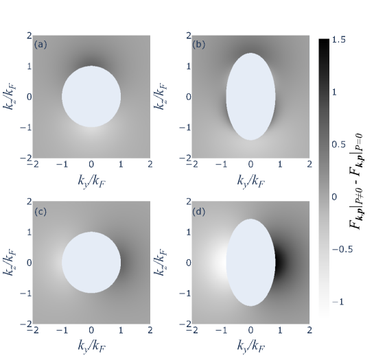
Figure 2: Numerical results for $\left.F_{\bm{k},\bm{p}}\right|_{P\neq 0}-\left.F_{\bm{k},\bm{p}}\right|_{P=0}$ in $k_{z}$-$k_{y}$ plane, where $\bm{p}\parallel\bm{P}$ and $F_{\bm{k},\bm{p}}$ is averaged over $\bm{p}$. (a) $C_{dd}=0,P_{z}=0.1k_{F}$, (b) $C_{dd}=1.5,P_{z}=0.1k_{F}$, (c) $C_{dd}=0,P_{y}=0.1k_{F}$, and (d) $C_{dd}=1.5,P_{y}=0.1k_{F}$.

In Fig. 3, we show the numerical results for the polaron energy calculated from Eq. (30) at the unitarity limit $a^{-1}=0$ for the DDI strength $C_{dd}=0-1.5$, and we also present the numerical values of the symbols in TABLE 2.

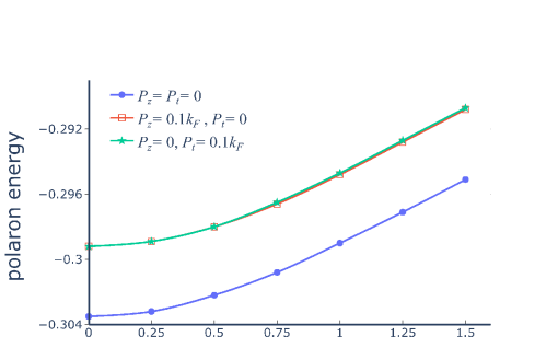
Figure 3: The DDI strength $C_{dd}$ dependence of the polaron energy $E(\bm{P})$ (in units of $k_{F}^{2}/M$) calculated for the total momenta $(P_{t},P_{z})=(0,0),(0,0.1),(0.1,0)$ (in units of $k_{F}$) at $M/m=1$ and the unitarity $a^{-1}=0$. The momentum cutoff used in numerical calculations is $\Lambda=100k_{F}$, with which enough convergence is found in the momentum integrals.

$C_{dd}$	$0$	$0.25$	$0.5$	$0.75$	$1.0$	$1.25$	$1.5$
$E(P_{t}=0,P_{z}=0)$	$-0.3035$	$-0.3032$	$-0.3022$	$-0.3008$	$-0.2990$	$-0.2971$	$-0.2951$
$E(P_{t}=0,P_{z}=0.1)$	$-0.2992$	$-0.2989$	$-0.2980$	$-0.2966$	$-0.2948$	$-0.2928$	$-0.2908$
$E(P_{t}=0.1,P_{z}=0)$	$-0.2992$	$-0.2989$	$-0.2980$	$-0.2965$	$-0.2947$	$-0.2927$	$-0.2907$

Table 2: The values of the polaron energy in Fig.3.

We note that the case of $C_{dd}=0$ reproduces the result of the spin imbalanced system obtained in the literature PhysRevA.74.063628 . These numerical results show that the binding energy of the polaron decreases with DDI strength by a small amount and that the polaron energy increases with increasing magnitude of the transverse and longitudinal momenta, $P_{t}$ and $P_{z}$, also by a small amount. We will examine the momentum-dependence of the polaron energy by evaluating the effective mass in the next subsection.

III.3 EFFECTIVE MASS

The effective mass, which characterizes the mobility of the polaron in the medium, has directional dependence because of the deformed shape of the Fermi surface by the DDI. In this paper, we adopt the definition of the effective mass based on the momentum expansion of the polaron energy:

$$E(\bm{P})=E(0)+\frac{P_{t}^{2}}{2M_{t}}+\frac{P_{z}^{2}}{2M_{z}}+{\mathcal{O}}(P^{4}),$$ (32)

where $M_{t}$ and $M_{z}$ are the transverse and longitudinal effective masses, respectively:

$$M_{t}^{-1}=\left.\frac{\partial^{2}E}{\partial P_{t}^{2}}\right|_{P=0},$$ (33)

$$M_{z}^{-1}=\left.\frac{\partial^{2}E}{\partial P_{z}^{2}}\right|_{P=0}.$$ (34)

In Fig. 4, we show the numerical results for the DDI dependence of the effective masses and present the numerical values of the symbols in TABLE 3. We have found from these results that the longitudinal mass is not so sensitive to the DDI, while the transverse one tends to decrease monotonically with the strength of the DDI. It is not straightforward to understand such directional dependence because whereas a polaronic cloud composed of excitations around the impurity generally acts to increase the polaron effective mass, additional effects due to the deformation of the Fermi surface produce anisotropy in the effective mass not only via change in the structure of the polaronic cloud as depicted in Fig. 2, but also via change in the density of states available for particles and holes in the medium. It should be noted that such an anisotropic effective mass has also been reported for Bose polarons in a dipolar BEC PhysRevA.89.023612 .

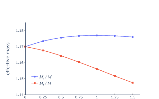
Figure 4: The DDI strength $C_{dd}$ dependence of the relative effective masses, $M_{z}/M$ and $M_{t}/M$. The parameters that characterize the polaronic state are set in the the same way as in Fig. 3.

$C_{dd}$	0	0.25	0.5	0.75	1.0	1.25	1.5
$M_{z}/M$	1.170	1.173	1.176	1.177	1.177	1.177	1.176
$M_{t}/M$	1.170	1.168	1.164	1.160	1.156	1.152	1.140
$M_{z}/M_{t}$	1.000	1.004	1.010	1.014	1.018	1.021	1.030

Table 3: The values of the effective masses in Fig.4 and the ratio $M_{z}/M_{t}$.

III.4 Momentum drag parameter

The change of the polaron effective masses from the impurity mass $M$ is attributable to the p-h excitations around the impurity, since they contribute to the kinetic term in (22) through the expectation value of the momentum of medium fermions:

$$\langle\hat{\bm{P}}\rangle =\sum_{\bm{q}}\bm{q}\langle a_{\bm{q}}^{\dagger}a_{\bm{q}}\rangle=\sum_{k>,p<}(\bm{k}-\bm{p})|F_{\bm{k},\bm{p}}|^{2}.$$ (35)

Then, let us define the drag parameter $\eta_{ij}$ via

$$\langle\hat{\bm{P}}\rangle_{i} =\eta(\bm{P})_{ij}P_{j}.$$ (36)

In this way, $\eta_{ij}$ measures the momentum-share of the p-h excitations accompanying the polaron via the wave function (31) that depends on $\bm{P}$ implicitly. On the basis of symmetry considerations, we may assume the diagonal form for the drag parameter:

$$\eta_{i}P_{i}=\langle\hat{\bm{P}}\rangle_{i}=\sum_{k>,p<}(k_{i}-p_{i})|F_{\bm{k},\bm{p}}|^{2},$$ (37)

where $\eta_{t}$ and $\eta_{z}$ are the transverse and longitudinal drag parameters.

TABLE 4 shows the DDI dependence of the drag parameters;

$C_{dd}$	$0$	$0.5$	$1.0$	$1.5$
$\eta_{z}(P_{t}=0,P_{z}=0.1)$	0.145	0.149	0.150	0.150
$\eta_{t}(P_{t}=0.1,P_{z}=0)$	0.145	0.142	0.135	0.129

Table 4: The DDI strength $C_{dd}$ dependence of the drag parameters calculated for the momentum $(P_{t},P_{z})=(0,0.1),(0.1,0)$ (in units of $k_{F}$). The parameters that characterize the polaronic state are set in the the same way as in Fig. 3.

the p-h excitations contribute to $13\%$–$15\%$ of the momentum of a slowly-moving polaron. Just like the case of the effective mass, the transverse drag parameter monotonically decreases with increasing $C_{dd}$ while the longitudinal one is less sensitive to $C_{dd}$ than the transverse one.

III.5 Medium density distribution

In the subsections above, we have studied the DDI-dependence of the polaron properties. As suggested in earlier investigations, however, the dipolar Fermi gas itself may be unstable toward a density collapse for sufficient strong DDI’s. The critical value of the DDI strength for the collapse is estimated to be $C_{dd}\simeq 2.4$ from the compressibility analysis in the variational method Sogo_2009 , as well as $C_{dd}\simeq 1.03$ from the analyses of collective modes Chan_2010 and zero sounds Ronen_2010 . In the present study, we cannot strictly discuss the possibility that such instability could be caused by a impurity injection into a marginally stable dipolar Fermi gas, since fermion-density fluctuations, which tend to develop in the presence of the DDI, are not incorporated in the calculation. Instead, we evaluate an enhancement of the medium density distribution around the impurity by treating the impurity as an external probe at position $\bm{x}$ and calculating the medium density distribution as a function of the relative distance from the impurity for $\bm{P}=0$ as 2016PhRvB..93t5144N ; PhysRevA.99.023601

$$n(\bm{r}-\bm{x}) =\langle S^{-1}\psi^{\dagger}(\bm{r})\psi(\bm{r})S\rangle$$

$$=\frac{1}{V}\sum_{\bm{q}_{1},\bm{q}_{2}}{\mathrm{e}}^{-i(\bm{q}_{2}-\bm{q}_{1})\cdot(\bm{r}-\bm{x})}\biggr{[}|F_{0}|^{2}\langle a^{\dagger}_{\bm{q}_{1}}a_{\bm{q}_{2}}\rangle+\left(F_{0}\sum_{k>,p<}F_{\bm{k},\bm{p}}^{*}\langle a^{\dagger}_{\bm{p}}a_{\bm{k}}a^{\dagger}_{\bm{q}_{1}}a_{\bm{q}_{2}}\rangle+\hbox{h.c.}\right)$$

$$\qquad\qquad\qquad\qquad\qquad\qquad\qquad\quad+\sum_{k>,p<}\sum_{k^{\prime}>,p^{\prime}<}F_{\bm{k},\bm{p}}^{*}F_{\bm{k}^{\prime},\bm{p}^{\prime}}\langle a^{\dagger}_{\bm{p}}a_{\bm{k}}a^{\dagger}_{\bm{q}_{1}}a_{\bm{q}_{2}}a^{\dagger}_{\bm{k}^{\prime}}a_{\bm{p}^{\prime}}\rangle\biggr{]}$$

$$=n_{f}+|F_{0}|^{2}\int_{k>,p<}\bar{F}_{\bm{k},\bm{p}}^{*}\biggr{[}2{\mathrm{e}}^{-i(\bm{p}-\bm{k})\cdot(\bm{r}-\bm{x})}+\int_{k_{2}>}\bar{F}_{\bm{k}_{2},\bm{p}}e^{-i(\bm{k}_{2}-\bm{k})\cdot(\bm{r}-\bm{x})}$$

$$\qquad\qquad\qquad\qquad\qquad\qquad\qquad\qquad\qquad-\int_{p_{2}<}\bar{F}_{\bm{k},\bm{p}_{2}}{\mathrm{e}}^{-i(\bm{p}-\bm{p}_{2})\cdot(\bm{r}-\bm{x})}\biggr{]},$$ (38)

where we have used the normalization condition (21), and introduced the scaled variables $\bar{F}_{\bm{k},\bm{p}}=VF_{\bm{k},\bm{p}}/F_{0}$ and the abbreviated notation for the integrals, $\int_{\bm{q}}\equiv\int{\rm d}^{3}q/(2\pi)^{3}$, etc. The distribution (38) is equivalent to the impurity-fermion density correlation function calculated, for instance, in residue ; imptrapfermion , which gives a Friedel oscillation in the spherically symmetric case. It should be noted that $F_{\bm{k},\bm{p}}$ is real and even for the transformation $k,p\rightarrow-k,-p$. Since the density distribution $n(\bm{r})$ diverges at $\bm{r}=0$ in the limit of the infinite momentum cutoff for $k>$ integrals, we have introduced a cutoff $\Lambda=2k_{F}$ in numerical integration, which is related to the effective range $r_{e}=\frac{4}{\pi\Lambda}$ in the impurity-medium interaction (see Appendix C for details).

Fig. 5 displays the medium density distribution along $z$-axis and $y$-axis.

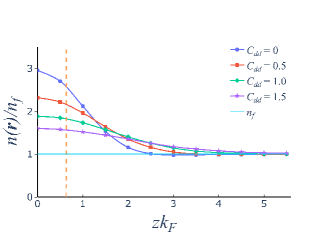
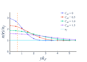
Figure 5: The medium density distribution for the longitudinal coordinate $z$ (left) and the vertical coordinate $y$ (right). The dashed line denotes the effective range. The parameters that characterize the polaronic state are $\Lambda=2k_{F}$, $M/m=1$, $a^{-1}=0$, and $\bm{x}=0$. Note that $n(\bm{r})$ approaches $n_{f}$ defined in Eq.(18), which corresponds to the density of a homogeneous system in the absence of the impurity, when $|\bm{r}|\to\infty$.

It is found from these figures that the medium density has a significant enhancement at the center of the Fermi polaron due to the attractive nature of the interaction, which is expected if the polaron is treated as a wave packet or a dilute gas cloud in reality, and that the enhanced area broadens as the Fermi surface deformation is enlarged for stronger DDI’s. It is interesting to note that the polaronic cloud is relatively narrow in the elongated direction of the Fermi surface, a feature that is consistent with the uncertainty principle.

Such a density enhancement implies that the increase in DDI strength $C_{dd}$ acts to expand the local area of the polaronic cloud and may eventually trigger a local instability of a dipolar Fermi gas, which is different from the instabilities predicted in Refs. Chan_2010 ; Ronen_2010 ; Kestner_2010 ; PhysRevA.84.053603 ; PhysRevA.91.023612 due to growth of density fluctuations in the long wavelength limit. Unlike droplet formation in a dipolar BEC Wenzel_2018 , however, such a local instability does not immediately lead to droplet formation in the dipolar Fermi gas. This is partly because in the present model Hamiltonian there is no genuine short-range repulsion among medium-fermions that can support the droplet.

IV Summary and outlook

We have studied the single polaron properties in a homogeneous dipolar Fermi gas using a Chevy-type variational method. The dipole-dipole interaction (DDI) in the Fermi gas medium causes a spheroidal deformation of the Fermi surface, which in turn leads to anisotropy in the polaron’s dispersion relation. We have investigated the DDI-dependence of various polaron properties at the unitarity limit of the impurity-medium interaction; the obtained results are summarized in Figs. 3–5 and in TABLES 2–4. We have found significant deviations from the case of no DDI: The effective mass and the momentum drag parameter for the transverse direction with respect to the polarization both decrease with increasing the strength of DDI, while those for the longitudinal direction are both less sensitive to the DDI strength than the transverse ones. All these behaviors are attributed to the influence of the deformation of the Fermi surface, which is elusive because such deformation affects not only the structure of the polaronic cloud as depicted in Fig. 2, but also the density of states available for particles and holes in the medium.

An interesting future direction related to the present work is the instability problem of a dipolar Fermi gas, which could be caused by the impurity injection. As shown in Sec. III.5, the impurity causes local enhancement of the medium density, which may eventually lead to a density collapse. Thus, if some repulsive forces exist to keep the system metastable against the collapse, a droplet formation might be expected PhysRevLett.89.050402 . Another possible direction of study is related to the correlation among impurities just mentioned above. Non-local effective interaction between two impurities, which can appear via, e.g., a long-range force mediated by fluctuations in the medium 2012PhRvA..85a3605G ; 2016PhRvB..93t5144N ; 2018JPSJ…87d3002N ; 2018PhRvL.121a3401C ; 2020PhRvL.124p3401E , is expected to provide a basis for further study of multi-impurity systems 2008PhRvL.100x0406B ; 2011PhRvA..84e1605G ; PhysRevA.102.051302 ; Mistakidis_2019 .

Appendix A Model single particle energy

In this appendix we examine the model single particle energy (14) that approximates the self-consistent single particle energy (11). We first summarize a variational method used in Sec. II.3 by writing down the number-conserving variational ansatz for the distribution function,

$$n_{\bm{q}}=\theta\left(k_{F}^{2}-\frac{1}{\beta}[q_{x}^{2}+q_{y}^{2}]-\beta^{2}q_{z}^{2}\right)$$

with $k_{F}=(6\pi^{2}n_{f})^{1/3}$, which is given by Eq. (12). Here, the parameter $\beta$ characterizes the deformation of the Fermi surface. Given the ansatz, the total energy can be derived as

$$\frac{E(\beta)}{V}=\frac{1}{m}n_{f}^{5/3}\left[C\left(\frac{2\beta}{3}+\frac{1}{3\beta^{2}}\right)-\frac{\pi}{3}C_{dd}I(\beta)\right]=\frac{1}{m}n_{f}^{5/3}{\mathcal{E}}(\beta),$$ (A.1 )

where $C=3(6\pi^{2})^{2/3}/10$ and the function $I(\beta)$ is given by

$$I(\beta)=\displaystyle\frac{6}{1-\beta^{3}}\left[1-\sqrt{\frac{\beta^{3}}{1-\beta^{3}}}\arctan{\left(\frac{1-\beta^{3}}{\beta^{3}}\right)}\right]-2.$$

In this variational method, the ground state energy and the optimal value of $\beta$ are determined by the stationary condition for the total energy, Eq. (A.1), with respect to $\beta$ at fixed $C_{dd}$. For non-interacting fermions ($C_{dd}=0$), $\beta$ equals unity, leading to a spherical Fermi surface. As the DDI strength increases, $\beta$ becomes less than one, leading to a prolate Fermi surface.

Let us turn to the model single particle energy consistent with the ansatz (12), which is written in terms of the optimal $\beta$ as

$$\epsilon_{\bm{q}}=\epsilon_{0}+\frac{\lambda^{2}}{2m}\left(\frac{1}{\beta}(q_{x}^{2}+q_{y}^{2})+\beta^{2}q_{z}^{2}\right),$$ (A.2 )

where

$$\epsilon_{0}=-\frac{(6\pi^{2})^{1/3}}{9\pi}\frac{k_{F}^{2}}{m}C_{dd}I(\beta)$$ (A.3 )

is the HF self-energy at ${\bm{q}}=0$ obtained by substituting the ansatz (12) into the right side of Eq. (11). Here, $\lambda$ is the curvature parameter of the single particle energy and is determined by the relationship

$$\epsilon_{F}=\epsilon_{0}+\frac{\lambda^{2}k_{F}^{2}}{2m},$$

where $\epsilon_{F}$ is given by $V^{-1}\partial E/\partial n_{f}|_{V}$ with $E$ given by Eq. (A.1). Thus the variational single particle energy in this procedure can be regarded as that of a quasiparticle with anisotropic effective masses $m_{z}/m=1/\beta^{2}\lambda^{2}$ and $m_{t}/m=\beta/\lambda^{2}$ because expression (A.2) can now be rewritten as

$$\epsilon_{\bm{q}}=\epsilon_{0}+\frac{1}{2m_{t}}(q_{x}^{2}+q_{y}^{2})+\frac{1}{2m_{z}}q_{z}^{2},$$ (A.4 )

where $\epsilon_{0}$ is still given by Eq. (A.3).

For $C_{dd}=1.0$, the deformation and curvature parameters can be obtained from the above procedure as $\beta=0.7769$ and $\lambda^{2}=1.0702$. The variational single particle energies, $\epsilon(0,0,q)$ and $\epsilon(q,0,0)$, calculated from Eq. (A.4) for such parameter values are plotted as dot-dashed line and dotted line in Fig. 6, respectively. Both of them agree with the self-consistent HF single particle energy below and around the Fermi energy, but clearly deviate from the HF result well above the Fermi energy. This deviation can be corrected in such a way as to reproduce the free-particle spectrum for large $q$, which is guaranteed by the self-consistent HF equation. Thus we employ the model single particle energy (14) with the momentum-dependent effective masses, which agrees well with the HF result even above the Fermi energy as shown in Fig. 6. We note that the value of $k_{c}$ has been determined to be $2.5k_{F}$ independently of the value of $C_{dd}$ in such a way that the model single particle energy (14) is consistent with the HF calculations.

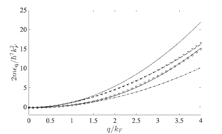
Figure 6: Same as Fig. 1 with additional plots of $\epsilon(0,0,q)$ (dot-dashed line) and $\epsilon(q,0,0)$ (dotted line) given by Eq. (A.4).

Appendix B Eigenvalue problem for polaron energy

From Eq. (28), one finds an equation for the auxiliary field $\chi_{\bm{p}}=F_{0}+\sum_{k>}F_{\bm{k},\bm{p}}$,

$$\chi_{\bm{p}}=F_{0}+\frac{1}{V}\sum_{k>}\frac{g\chi_{\bm{p}}}{E-\Omega_{\bm{k},\bm{p};\bm{P}}}.$$ (B.1 )

Plugging this into Eq. (27), one obtains

$$\frac{g}{V}\sum_{p}\frac{g^{-1}F_{0}}{g^{-1}-\frac{1}{V}\sum_{k>}\frac{1}{E-\Omega_{\bm{k},\bm{p};\bm{P}}}}=\biggr{(}E-\frac{P^{2}}{2M}\biggr{)}F_{0},$$ (B.2 )

which leads to Eq. (31).

Appendix C Effective range

We derive a relation between the momentum cutoff and the effective range. From the LS equation, the two-body $T$-matrix satisfies

$$T(\bm{k},\bm{k}^{\prime},\omega_{+})=g\gamma_{\bm{k}}\gamma_{\bm{k}^{\prime}}+\frac{g}{V}\sum_{\bm{p}}\frac{\gamma^{2}_{\bm{p}}}{\omega_{+}-\bm{p}^{2}/2m_{r}}T(\bm{p},\bm{k}^{\prime},\omega_{+}),$$ (C.1 )

where we take a cutoff $\Lambda$ via

$$\gamma_{\bm{k}}=\theta(\Lambda-|\bm{k}|).$$ (C.2 )

If we set

$$T(\bm{k},\bm{k}^{\prime},\omega_{+})=\gamma_{\bm{k}}t(\omega_{+})\gamma_{\bm{k}^{\prime}},$$ (C.3 )

then

$$t(\omega_{+})=g\biggr{[}1-\frac{g}{V}\sum_{\bm{p}}^{\Lambda}\frac{1}{\omega_{+}-p^{2}/2m_{r}}\biggr{]}^{-1}.$$ (C.4 )

Since the scattering amplitude $f(\bm{k})$ is related to the $T$-matrix as

$$f(\bm{k})=-\frac{m_{r}}{2\pi}T(\bm{k},\bm{k},k^{2}/2m_{r}+i\delta),$$ (C.5 )

we obtain from Eqs. (C.3) and (C.4)

$$f(\bm{k}) =-\frac{m_{r}}{2\pi}\gamma_{\bm{k}}g\biggr{[}1+\frac{g}{V}\sum_{\bm{p}}^{\Lambda}\frac{1}{p^{2}/2m_{r}-k^{2}/2m_{r}-i\delta}\biggr{]}^{-1}$$

$$=-\frac{m_{r}}{2\pi}\gamma_{\bm{k}}g\biggr{[}1+\frac{gm_{r}}{\pi^{2}}\biggr{(}\Lambda-k\tanh^{-1}\biggr{(}\frac{k}{\Lambda}\biggr{)}+\frac{i\pi k}{2}\biggr{)}\biggr{]}^{-1},$$ (C.6 )

where we have used

$$\frac{1}{V}\sum_{\bm{p}}^{\Lambda}\frac{1}{p^{2}/2m_{r}-k^{2}/2m_{r}-i\delta} =\frac{2m_{r}}{2\pi^{2}}\int_{0}^{\Lambda}dp\frac{p^{2}}{p^{2}-k^{2}-i\delta}$$

$$=\frac{m_{r}}{\pi^{2}}\biggr{(}\Lambda-k\tanh^{-1}\biggr{(}\frac{k}{\Lambda}\biggr{)}+\frac{i\pi k}{2}\biggr{)}.$$ (C.7 )

The scattering amplitude can be also written in terms of the $s$-wave scattering length $a$ and effective range $r_{e}$ as

$$f(\bm{k})=-\frac{1}{a^{-1}-r_{e}k^{2}/2+ik},$$ (C.8 )

so we obtain

$$-a^{-1}+\frac{1}{2}r_{e}k^{2}=-\theta(\Lambda-|\bm{k}|)\frac{2\pi}{m_{r}}\biggr{[}g^{-1}+\frac{m_{r}}{\pi^{2}}\biggr{(}\Lambda-k\tanh^{-1}\biggr{(}\frac{k}{\Lambda}\biggr{)}\biggr{)}\biggr{]}.$$ (C.9 )

Finally, comparison of the $O(k^{2})$ terms in the left and right sides of Eq. (C.9), which can be made by using $\tanh^{-1}(k/\Lambda)\approx k/\Lambda+O(k^{3})$, leads to the relation between the effective range and the cutoff,

$$r_{e}=\frac{4}{\pi\Lambda}.$$ (C.10 )