Investigating the Robustness of Artificial Intelligent Algorithms with Mixture Experiments

Abstract

Artificial intelligent (AI) algorithms, such as deep learning and XGboost, are used in numerous applications including computer vision, autonomous driving, and medical diagnostics. The robustness of these AI algorithms is of great interest as inaccurate prediction could result in safety concerns and limit the adoption of AI systems. In this paper, we propose a framework based on design of experiments to systematically investigate the robustness of AI classification algorithms. A robust classification algorithm is expected to have high accuracy and low variability under different application scenarios. The robustness can be affected by a wide range of factors such as the imbalance of class labels in the training dataset, the chosen prediction algorithm, the chosen dataset of the application, and a change of distribution in the training and test datasets. To investigate the robustness of AI classification algorithms, we conduct a comprehensive set of mixture experiments to collect prediction performance results. Then statistical analyses are conducted to understand how various factors affect the robustness of AI classification algorithms. We summarize our findings and provide suggestions to practitioners in AI applications.

Keywords: Convolutional Neural Network; Deep Learning; Design of Experiments; Imbalance Samples; Safety of AI Systems; XGBoost.

1 Introduction

1.1 Background

Machine learning (ML) and deep learning (DL) algorithms are widely used in many artificial intelligent (AI) applications such as computer vision (Hashimoto et al.,, 2019), autonomous driving (Tian et al.,, 2018), and medical diagnostics (Quer et al.,, 2017). There is a growing interest in investigating the robustness of AI algorithms (Dietterich,, 2017; Silva and Najafirad,, 2020; Hamon et al.,, 2020), as it is highly related to the safety of AI systems (Amodei et al.,, 2016). The robustness of AI algorithms often concerns how the performance of the algorithm may change when the training and test datasets are of certain differences (Xu et al.,, 2012). For example, adding noise into the training data can change the prediction performance of the AI algorithms to some extent. The robustness of the AI algorithms heavily relies on how the algorithm is trained and how the algorithm is evaluated on the test dataset of interest. In this work, we focus on investigating the robustness of classification algorithms as many artificial intelligent (AI) systems involve classification. The proposed framework, however, can be extended to study the robustness for AI algorithms beyond classification.

A robust classification algorithm is expected to have high accuracy and low variability under various scenarios. The robustness of the classification algorithm can be affected by a wide range of factors, such as the composition of training dataset, the change of distribution in the training and test datasets, the chosen prediction algorithm, and so on. In the training stage, AI algorithms often rely on a large number of data points. However, in many real-world applications, data for classification can be highly imbalanced in which data points from a particular class label overwhelmingly dominate data points from other class labels. It is crucial to understand how the performance of AI classification algorithms is affected by the class label imbalance in the training data. Moreover, when the distribution of test data deviates away from the distribution of the training data, such distribution changes can also largely affect the robustness of the classification algorithms (Kuleshov and Liang,, 2015). This lack of robustness has direct application to deployed algorithms used on data sets whose composition may differ from the original training data set.

In this paper, we use the idea of design of experiments (Wu and Hamada,, 2011) to systematically investigate the robustness of classification algorithms with respect to: (1) the class label imbalance in the training data; and (2) the distribution change between training and test data regarding the proportions of class labels. In particular, our key idea is to use the mixture experimental design (Cornell,, 2011) for the proportions of class labels in the training data, such that the robustness of the AI classification algorithms can be investigated in a systematic manner. Here the robustness of a classification algorithm is characterized by the mean and standard deviation of the areas under the receiver operating characteristic curves (AUC) for each class label (Yuan and Bar-Joseph,, 2019). We also study a wide range of other factors that can affect the robustness, including the distributional changes between the training data and the test data, different classification algorithms, and datasets from different applications. The convolutional neural network (CNN) (Kim,, 2014) and XGBoost (Chen et al.,, 2015) are adopted as two representative AI classification algorithms. Based on the classification performance results collected from the designed mixture experiments, statistical analyses are conducted to reveal some interesting findings on the robustness of AI classification algorithms. It is worth to remarking that the proposed framework can be extended to including more factors for investigating the robustness of the AI algorithms, and can also be used to study other characteristics of the AI algorithms, such as the transparency of the AI systems (Hamon et al.,, 2020).

1.2 Related Literature

In a typical mixture experiment (Cornell,, 2011), the design variables under study are the proportions of mixture components in a blend, with their summation equal to unity. A common objective is to investigate how the changes in the proportions of mixture components would affect the response outcomes (Piepel and Cornell,, 1994). The mixture experiments have been used in many agriculture and engineering applications (Kang et al.,, 2011, 2016; Shen et al.,, 2020). In our work, we adopt the idea of mixture experiments to study how the proportions of class labels would affect the performance of the AI classification algorithms. Among various AI classification algorithms, we consider the convolutional neural network (CNN) and the XGboost as the two representative algorithms. The CNN is a popular deep learning algorithm for classification, where the input variables are tensors (Goodfellow et al.,, 2016). Generally, the CNN uses convolution in place of general matrix multiplication in its perception layers. In contrast, XGboost is one efficient classification algorithm when the input contains numerical and categorical variables. The XGBoost stands for the Extreme Gradient Boosting, which is a parallel tree boosting method with efficient gradient-based optimization. Both CNN and XGboost are widely used in various application areas (Parsa et al.,, 2020). With the consideration of mixture experiments for the proportions of class labels, our approach is to provide a comprehensive understanding on the performance of these two classification algorithms.

The robustness of AI algorithms has attracted a large amount of attention in the machine learning community (Tsipras et al.,, 2018). There is a broad spectrum regarding the robustness of AI algorithms, including adversarial robustness, robust learning, robust models, robustness to distributional shift, etc. In the robust learning, a key interest is to redesign the learning procedure so that the algorithm is robust against malicious actions (Madry et al.,, 2017; Zantedeschi et al.,, 2017). Robust procedures include better training procedures against adversarial examples, as well as a better mathematical foundation of the algorithms by adopting techniques from statistics and optimization, such as robust statistic inference (Huber,, 2004; Lozano et al.,, 2013) and robust optimization (Ben-Tal et al.,, 2009). In the area of deep learning, some research work has focused on investigating the adversarial robustness (Dvijotham et al.,, 2018; Xiang et al.,, 2018; Gehr et al.,, 2018; Wong and Kolter,, 2018). It is known that neural network models are vulnerable to adversarial examples. That is, perturbing inputs that are very similar to some regular inputs could result in the output being dramatically different (Szegedy et al.,, 2013). For example, Tjeng et al., (2017) proposed a mixed integer programming method to examine the vulnerability of neural networks to such adversarial examples. A useful framework for certifying the robustness of CNNs against adversarial examples is discussed in Boopathy et al., (2019). The scope of our work is to use a framework of experimental design to investigate the robustness of AI algorithms against the class label imbalance in the training data and the distribution change on proportions of class labels between the training and test data.

1.3 Overview

The rest of the paper is organized as follows. Section 2 describes the proposed framework, including the response variables, the experimental factors, design runs, data collection and the modeling method. Section 3 reports the analysis results of experimental data. Section 4 contains some concluding remarks.

2 The Proposed Framework

2.1 Design Factors and Response Variables

Let us consider a multi-class classification with $m$ classes (labels). The accuracy of a classification algorithm can be measured by various performance measures, such as the misclassification error, false positive rate (FPR), $F_{1}$ score, etc. Note that the classification rule of a classification algorithm often depends on the setting of the classification threshold (Yuan and Bar-Joseph,, 2019). Among various performance measures, the area under the receiver operating characteristic curve (AUC) provides an aggregate measure of prediction accuracy for all possible thresholds. For a multi-class classification problem, one can obtain the AUC for each class label. To characterize the robustness of a classification algorithm, we consider two types of performance measures based on the AUC’s. The first one is the sample mean of the AUC values of $m$ classes, and the second one is the logarithm of the standard deviation of the AUC values from $m$ classes.

To investigate the robustness of the AI classification algorithms, we consider a mixture experiment on proportions of class label in the training dataset with several covariate variables such as different algorithms and different datasets of interest. Specifically, let $(x_{1},x_{2},\ldots,x_{m})$ be the proportions of class labels $\{1,\ldots,m\}$ in the training dataset. Note that $x_{1}+x_{2}+\cdots+x_{m}=1$ and $x_{j}\in[0,1]$ for $j=1,\ldots,m$. Suppose that there are $h$ covariate variables, $z_{1},\ldots,z_{h}$, for the mixture experiment. In our specific experimental setting, we consider two covariate variables $z_{1}$ and $z_{2}$, each with two levels. In particular, $z_{1}$ is a two-level factor that represents two different algorithms: the CNN algorithm and the XGboost algorithm. That is,

$$z_{1}=\begin{cases}1,&\text{if the XGboost algorithm is used},\\ 0,&\text{if the CNN algorithm is used}.\end{cases}$$

The $z_{2}$ variable is a two-level factor that represents two different dataset of interests: the KEGG dataset and the Bone Marrow dataset. That is,

$$z_{2}=\begin{cases}1,&\text{if the KEGG dataset is used},\\ 0,&\text{if the Bone Marrow dataset is used}.\end{cases}$$

The above two datasets are used in Yuan and Bar-Joseph, (2019) for the classification of the single cell RNA sequencing (scRNA-seq) expression. In Yuan and Bar-Joseph, (2019), the scRNA-seq data are converted into the normalized empirical probability distribution functions (NEPDF) between gene pairs as the input matrix and the CNN is applied for classification. The KEGG dataset is derived from the Kyoto Encyclopedia of Genes and Genomes (KEGG) as pathway datasets of study (Wixon and Kell,, 2000). The Bone Marrow dataset denotes the bone marrow derived macrophage scRNA-seq as the dataset of study (Orlic et al.,, 2001). The KEGG dataset contains $92{,}472$ observations and the Bone Marrow dataset has $80{,}253$ observations. Both datasets have $m=3$ classes with class proportions equally distributed, i.e., each class contains one third of observations. The details about the two datasets and their pre-processing can be found in (Yuan and Bar-Joseph,, 2019).

2.2 Design Construction and Runs

Because the datasets of interest have three class labels, we consider a modified simple centroid design for mixture experiment for $x_{1},x_{2},\ldots,x_{m}$ with $m=3$. A simple centroid design usually has $2^{m}-1$ points, including $m$ pure components (e.g., (0,0,1)), $\tbinom{m}{2}$ binary points (e.g., (0,1/2,1/2)) and $\tbinom{m}{3}$ ternary mixture (e.g., (1/3,1/3,1/3)). When $m=3$, there are seven different settings of proportions of class labels for the training dataset, as shown in Figure 1.

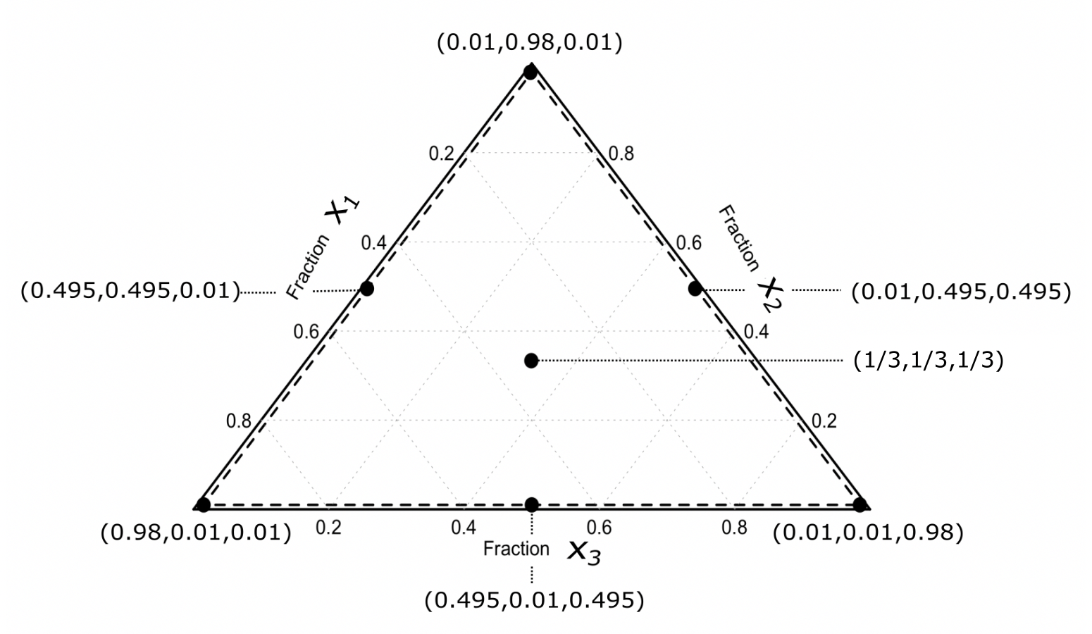
Figure 1: Illustration of seven settings of proportions of class labels in the training dataset. The dashed lines illustrate the restriction on the minimal value of a class proportion larger than 0.01, i.e., $x_{j}\geq 0.01$.

With the consideration of the covariate variables $z_{1}$ and $z_{2}$ with two-levels, we use the cross-array between the mixture design of $x_{1},x_{2},x_{3}$ and the full factorial design of $z_{1}$ and $z_{2}$. The design matrix of our proposed method is shown in Table 1.

Table 1: The 28-run mixture design with 2 covariate factors.

Run	$x_{1}$	$x_{2}$	$x_{3}$	$z_{1}$	$z_{2}$		Run	$x_{1}$	$x_{2}$	$x_{3}$	$z_{1}$	$z_{2}$
1	0.01	0.01	0.98	1	1		15	0.01	0.01	0.98	0	1
2	0.01	0.98	0.01	1	1		16	0.01	0.98	0.01	0	1
3	0.98	0.01	0.01	1	1		17	0.98	0.01	0.01	0	1
4	0.01	0.495	0.495	1	1		18	0.01	0.495	0.495	0	1
5	0.495	0.01	0.495	1	1		19	0.495	0.01	0.495	0	1
6	0.495	0.495	0.01	1	1		20	0.495	0.495	0.01	0	1
7	1/3	1/3	1/3	1	1		21	1/3	1/3	1/3	0	1
8	0.01	0.01	0.98	1	0		22	0.01	0.01	0.98	0	0
9	0.01	0.98	0.01	1	0		23	0.01	0.98	0.01	0	0
10	0.98	0.01	0.01	1	0		24	0.01	0.01	0.98	0	0
11	0.01	0.495	0.495	1	0		25	0.01	0.495	0.495	0	0
12	0.495	0.01	0.495	1	0		26	0.495	0.01	0.495	0	0
13	0.495	0.495	0.01	1	0		27	0.495	0.495	0.01	0	0
14	1/3	1/3	1/3	1	0		28	1/3	1/3	1/3	0	0

Note that our goal is to investigate the robustness of AI classification algorithms on their prediction performance. For the experimental setting of $x_{1},x_{2},x_{3}$, the proportions of class labels in the training dataset, it is not practical to set the proportion of a class label to be zero, i.e., $x_{j}=0$ for some $j$. Under this consideration, we modify the simple centroid design to restrict the minimum value of class proportion to be larger than 0.01, i.e., $x_{j}\geq 0.01$, which is illustrated by the dashed lines in Figure 1.

To calculate the classification accuracy, a test dataset is often needed. The proportions of class labels in the test dataset also can have an effect on the classification performance of the algorithms. Often time, we assume that the training and test datasets have the same distributions on the proportion of class labels. In practice, the distribution of proportions of class labels in the test dataset can be different from that in the training dataset. To comprehensively evaluate the robustness of the AI classification algorithm, we will alter the distribution of proportions of class labels in the test dataset to be possibly different from the distribution of class proportions in the training dataset. Specifically, three scenarios for the test dataset are considered, which are listed as follows.

• Balanced Scenario: The proportions of class labels in the test dataset are equal in each class, regardless of the proportions of class labels in the training dataset.

• Consistent Scenario: The proportions of class labels in the test dataset are the same as the proportions of class labels in the training dataset.

• Reverse Scenario: The proportion of class labels in the test dataset is in a reverse pattern as the proportion of class labels in the training dataset.

In the Reverse Scenario, if the proportion of a class label is high in the training dataset, then the proportion of this class label is set to be low in the test dataset. Table 2 shows the three scenarios of proportions of class labels between the training and test dataset.

Table 2: Three scenarios of proportions of class labels for forming the test dataset.

Balanced Scenario
Training	$x_{1}$	$x_{2}$	$x_{3}$		Test	$x_{1}$	$x_{2}$	$x_{3}$
	0.01	0.01	0.98			1/3	1/3	1/3
	0.01	0.98	0.01			1/3	1/3	1/3
	0.98	0.01	0.01			1/3	1/3	1/3
	0.01	0.495	0.495			1/3	1/3	1/3
	0.495	0.01	0.495			1/3	1/3	1/3
	0.495	0.495	0.01			1/3	1/3	1/3
	1/3	1/3	1/3			1/3	1/3	1/3
Consistent Scenario
Training	$x_{1}$	$x_{2}$	$x_{3}$		Test	$x_{1}$	$x_{2}$	$x_{3}$
	0.01	0.01	0.98			0.01	0.01	0.98
	0.01	0.98	0.01			0.01	0.98	0.01
	0.98	0.01	0.01			0.98	0.01	0.01
	0.01	0.495	0.495			0.01	0.495	0.495
	0.495	0.01	0.495			0.495	0.01	0.495
	0.495	0.495	0.01			0.495	0.495	0.01
	1/3	1/3	1/3			1/3	1/3	1/3
Reverse Scenario
Training	$x_{1}$	$x_{2}$	$x_{3}$		Test	$x_{1}$	$x_{2}$	$x_{3}$
	0.01	0.01	0.98			0.495	0.495	0.01
	0.01	0.98	0.01			0.495	0.01	0.495
	0.98	0.01	0.01			0.01	0.495	0.495
	0.01	0.495	0.495			0.98	0.01	0.01
	0.495	0.01	0.495			0.01	0.98	0.01
	0.495	0.495	0.01			0.01	0.01	0.98
						∗0.01	0.01	0.98
	1/3	1/3	1/3			∗0.01	0.98	0.01
						∗0.98	0.01	0.01
∗Randomly select one from the three proportion settings.

Note that for all experimental runs, we keep the size of the training dataset to the same with $n_{tr}=10\%\mbox{{ of the full dataset}}$, and keep the size of the test dataset to be the same with $n_{ts}=25\%\mbox{{ of the full dataset}}$. Here, we make the size of the test dataset larger than that of the training dataset for the following considerations. First, it allows the evaluation of classification performance at the test datasets being more valid, avoid the potential variation due to the small sample size. Second, a relatively smaller size of the training dataset could better serve the purpose of investigating the robustness of the algorithms. In the full datasets of the KEGG (of the size $92{,}472$ observations) and Bone Marrow (of the size $80{,}253$ observations), the class proportions are equally distributed, i.e., each label having one third of the full data. In each experimenting run, when forming the training dataset, we randomly sample with replacement from the full dataset in each class label based on the proportion setting $(x_{1},x_{2},x_{3})$ for training. The use of sampling with replacement for forming the training dataset is to simulate the possible duplicated data points in the real practice (Li et al.,, 2020). For forming the test dataset, we randomly sample without replacement from the remaining data in each class label based on the proportion setting $(x_{1},x_{2},x_{3})$ for test. We use the sampling without replacement to make each data point unique in the test dataset.

To illustrate how data points with its percentage for each label are composed in both training and test datasets, we show a toy example as follows. Suppose that there are $N=10000$ observations in the full dataset with three class proportions equally distributed. Then we set the size of training dataset to be fixed at $n_{tr}=10\%\cdot N=1000$, while the size of test dataset is set to be $n_{ts}=25\%\cdot N=2500$. Assume that in one experimental run, the proportions of class labels in the training dataset is designed to be $(x_{1},x_{2},x_{3})=(0.01,0.01,0.98)$, and the proportions of class labels in the test dataset is designed to be $(x_{1},x_{2},x_{3})=(0.01,0.01,0.98)$. Based on the full dataset, the training dataset is composed by randomly sampling $(10,10,980)$ observations from the three classes of data points, respectively. Then using the remaining data points, the test dataset is composed by randomly sampling $(25,25,2450)$ observations from the three classes of the remaining data points, respectively.

2.3 Data Collection and Modeling Method

As shown in Table 1, there are 28 treatments (i.e., runs) in the proposed design under each scenario of test data. For each treatment, we conduct three replications. All experiments were carried out on a DGX-2 machine which is a product of NVIDIA focusing on deep learning implementation. On average, each experiment takes around 30 minutes in computation. The outcome of an experiment is the AUC value of each class on the test dataset by a selected classification algorithm (CNN or XGboost), which is estimated based on the training data. Note that for the classification algorithms, the input of the CNN model is the matrix of the normalized empirical probability distribution functions (NEPDF) between gene pairs, which is an image-type input. We adopt the same implementation of the CNN as in Yuan and Bar-Joseph, (2019). While in the implementation of XGboost, the inputs contain the column sum, row sum, and the trace of the matrix of NEPDFs. In fact, column sums and row sums are the marginal empirical distribution of each gene in the pair, and the trace is also a summary of the matrix.

Based on the AUC value of each class, denoted as $\eta_{1},\ldots,\eta_{m}$, then the averaged AUC (mean AUC) can be obtained as

$$\bar{\eta}=\frac{1}{m}\sum_{j=1}^{m}\eta_{j}\ ,$$

and the logarithm of the standard deviation (Log SD) can be obtained as

$$\textrm{Log SD}=\log\left(\left[\frac{1}{m-1}\sum_{j=1}^{m}(\eta_{j}-\bar{\eta})^{2}\right]^{1/2}\right)\,.$$

When the outcomes of designed experiments (i.e., the collected data) are obtained, our key interest is to conduct proper statistical modeling to understand how the design factors (class label proportions $x_{1},\ldots,x_{m}$, the algorithms, and the datasets of interest) affect the response (the classification accuracy). Note that we have three test scenarios, the Consistent Scenario, the Balanced Scenario, and the Reverse Scenario. We will conduct the statistical analysis of experimental data separately for each scenario.

Given a given test scenario, we denote $(x_{i1},x_{i2},\ldots,x_{im})$ as the proportions of class labels of the training dataset for the $i$th run, and $z_{ik}$ to be the level of covariate variable $z_{k}$ for the $i$th run. Let $y_{i}$ be the corresponding response variable, which can be the mean AUC or the Log SD. Let $n$ be the sample size of the collected data under a given test scenario. To analyze the collected data $(y_{i},x_{i1},x_{i2},\ldots,x_{im},z_{i1},\ldots,z_{ih})$, we consider the following regression model,

$$y =\sum_{j=1}^{m}(\beta_{j}+\sum_{k=1}^{h}\gamma_{kj}z_{k})x_{j}+\sum_{j<j^{\prime}}\beta_{jj^{\prime}}x_{j}x_{j^{\prime}}+\sum_{k<k^{\prime}}\delta_{kk^{\prime}}z_{k}z_{k^{\prime}}+\epsilon$$

$$=\sum_{j=1}^{m}\beta_{j}x_{j}+\sum_{j<j^{\prime}}\beta_{jj^{\prime}}x_{j}x_{j^{\prime}}+\sum_{k=1}^{h}\sum_{j=1}^{m}\gamma_{kj}z_{k}x_{j}+\sum_{k<k^{\prime}}\delta_{kk^{\prime}}z_{k}z_{k^{\prime}}+\epsilon,$$ (1)

where $\beta_{j}$’s and $\beta_{jj^{\prime}}$’s are regression coefficients for the main and interaction terms of the label proportions, respectively. The $\gamma_{kj}$’s are the regression coefficients for the interaction between class label proportions and the covariate variables, and $\delta_{kk^{\prime}}$’s are the regression coefficients for the interactions of the covariate variables. The $\epsilon\sim\textrm{N}(0,\sigma^{2})$ is the error term. Here, the model does not include the high-order interaction terms to keep the model parsimonious.

Denote $\beta$ to be the vector of coefficients including $\beta_{0}$, $\beta_{j}$’s and $\beta_{jj^{\prime}}$’s. Similarly, we define $\gamma$ and $\delta$ to be the vectors of coefficients for $\gamma_{kj}$’s and $\delta_{kk^{\prime}}$’s, respectively. For the parameter estimation, we adopt the maximum likelihood estimation, which is equivalent to the least squares estimation in our problem. That is,

$$\footnotesize(\hat{\mbox{\boldmath$\beta$\unboldmath}},\hat{\mbox{\boldmath$\gamma$\unboldmath}},\hat{\mbox{\boldmath$\delta$\unboldmath}})=\arg\min_{\mbox{\boldmath$\beta$\unboldmath},\mbox{\boldmath$\gamma$\unboldmath},\mbox{\boldmath$\delta$\unboldmath}}\sum_{i=1}^{n}\left(y_{i}-\sum_{j=1}^{m}\beta_{j}x_{ij}-\sum_{j<j^{\prime}}\beta_{jj^{\prime}}x_{ij}x_{ij^{\prime}}-\sum_{k=1}^{h}\sum_{j=1}^{m}\gamma_{kj}z_{k}x_{ij}-\sum_{k<k^{\prime}}\delta_{kk^{\prime}}z_{ik}z_{ik^{\prime}}\right)^{2}.$$

Note that the model in (2.3) does not include an intercept term because the class label proportions sum up to one, i.e., $x_{1}+\cdots+x_{m}=1$. The model in (2.3) also does not include the quadratic term of label proportions since it can be linearly expressed by its main effect and its interactions with other class label proportions, i.e., $x_{j}^{2}=x_{j}-\sum_{j^{\prime}\neq j}x_{j}x_{j^{\prime}}$. Moreover, the model in (2.3) does not include the main effect of the covariate factor since it can be linearly expressed by the interactions between class label proportions and the covariate variables, i.e., $z_{k}=z_{k}x_{1}+\cdots+z_{k}x_{m}$. To make proper inference on the contribution of $z_{k}$ in the estimated model, one could include $z_{k}$ into the regression model in (2.3), which leads to the following terms in the model,

$$\gamma_{k1}z_{k}x_{1}+\gamma_{k2}z_{k}x_{2}+\cdots+\gamma_{km}z_{k}x_{m}+\gamma_{k}z_{k}$$

$$=(\gamma_{k1}+\gamma_{k})z_{k}x_{1}+(\gamma_{k2}+\gamma_{k})z_{k}x_{2}+\cdots+(\gamma_{km}+\gamma_{k})z_{k}x_{m}.$$ (2)

By imposing the sum-to-zero constraint (Wu and Hamada,, 2011) for model identifiability, we have

$$(\gamma_{k1}+\gamma_{k})+\cdots+(\gamma_{km}+\gamma_{k})=0\Rightarrow\gamma_{k}=-\frac{1}{m}(\gamma_{k1}+\gamma_{k2}+\cdots+\gamma_{km}).$$

In this sense, we make inference on $z_{k}$ based on the linear combination of $\hat{\gamma}_{kj}$’s through $\frac{1}{m}\sum_{j=1}^{m}\hat{\gamma}_{kj}$. It is worth to pointing out that one could also impose the baseline constraint, such as $\gamma_{k}=0$ in (2.3), then it becomes the original model in (2.3).

Moreover, based on the estimated model, it is useful to quantify the impact of the predictor variables to the response. Here we adopt the SHAP (SHapley Additive exPlanations) approach (Lundberg and Lee,, 2017) to quantitatively assess the impact of predictor variables to the response. The Shapley value, based on the cooperative game theory (Shapley,, 1953), can be applied in a wide variety of models and is not affected by the unit of measurement. The SHAP method assigns each predictor variable a Shapley value of importance for the predictive model. For the linear model in (2.3), the SHAP has an explicit form. The detailed explanations of the Shapely formula under the linear model can be found in the appendix. Denote $\phi_{i}^{(x_{j})}$ as the importance of the label proportion variable $x_{j}$ to the model output for individual observation $i$. Similarly, we can define $\phi_{i}^{(z_{k}x_{j})}$, $\phi_{i}^{(x_{j}x_{j^{\prime}})}$, $\phi_{i}^{(z_{k}z_{k^{\prime}})}$. For the $i$th observation in our proposed model, the importance of predictor variables $x_{j}$’s, $x_{j}x_{j^{\prime}}$’s, $z_{k}x_{j}$’s, and $z_{k}z_{k}^{\prime}s$ have the following forms:

$$\phi_{i}^{(x_{j})} =\beta_{j}\Big{(}x_{ij}-\frac{1}{n}\sum_{i=1}^{n}x_{ij}\Big{)},\quad j=1,\ldots,m;$$

$$\phi_{i}^{(x_{j}x_{j^{\prime}})} =\beta_{jj^{\prime}}\Big{(}x_{ij}x_{ij^{\prime}}-\frac{1}{n}\sum_{i=1}^{n}x_{ij}x_{ij^{\prime}}\Big{)},\quad j<j^{\prime},j=1,\ldots,m,j^{\prime}=1,\ldots,m;$$

$$\phi_{i}^{(z_{k}x_{j})} =\gamma_{kj}\Big{(}z_{ik}x_{ij^{\prime}}-\frac{1}{n}\sum_{i=1}^{n}z_{ik}x_{ij}\Big{)},\quad k=1,\ldots,h,j=1,\ldots,m;$$

$$\phi_{i}^{(z_{k}x_{j})} =\delta_{kk^{\prime}}\Big{(}z_{ik}z_{ik^{\prime}}-\frac{1}{n}\sum_{i=1}^{n}z_{ik}z_{ik}\Big{)},\quad k<k^{\prime},k=1,\ldots,h,j^{\prime}=1,\ldots,h.$$

The SHAP can also be used to quantify the overall impact of each predictor variable by using the average absolute impact on model output magnitude as the evaluation metric; i.e.,

$$\phi^{(x_{j})} =\frac{1}{n}\sum_{i=1}^{n}|\phi_{i}^{(x_{j})}|,\quad j=1,\ldots,m;$$ (3)

$$\phi^{(x_{j}x_{j^{\prime}})} =\frac{1}{n}\sum_{i=1}^{n}|\phi_{i}^{(x_{j}x_{j^{\prime}})}|,\quad j<j^{\prime},j=1,\ldots,m,j^{\prime}=1,\ldots,m;$$ (4)

$$\phi^{(z_{k}x_{j})} =\frac{1}{n}\sum_{i=1}^{n}|\phi_{i}^{(z_{k}x_{j})}|,\quad k=1,\ldots,h,j=1,\ldots,m;$$ (5)

$$\phi^{(z_{k}x_{j})} =\frac{1}{n}\sum_{i=1}^{n}|\phi_{i}^{(z_{k}x_{j})}|,\quad k<k^{\prime},k=1,\ldots,h,j^{\prime}=1,\ldots,h.$$ (6)

These metrics, $\phi^{(x_{j})}$’s, $\phi^{(x_{j}x_{j^{\prime}})}$’s,$\phi^{(z_{k}x_{j})}$’s, and $\phi^{(z_{k}x_{j})}$’s will be used to assess and compare these impacts to the response in the next section.

3 Data Analysis

In this section, we conduct the modeling and data analysis when the response variable is the mean AUC and the Log SD, respectively. In our analysis with $m=3$ class labels and $h=2$ covariate variables, the collected data of experiments are $(y_{i},x_{i1},x_{i2},x_{i3},z_{1i},z_{2i}),i=1,\ldots,n$. Then the model in (2.3) is expressed as,

$$y_{i}= \beta_{1}x_{i1}+\beta_{2}x_{i2}+\beta_{3}x_{i3}+\beta_{12}x_{i1}x_{i2}+\beta_{13}x_{i1}x_{i3}+\beta_{23}x_{i2}x_{i3}$$ (7)

$$+\gamma_{11}z_{i1}x_{i1}+\gamma_{12}z_{i1}x_{i2}+\gamma_{13}z_{i1}x_{i3}+\gamma_{21}z_{i2}x_{i1}+\gamma_{22}z_{i2}x_{i2}+\gamma_{23}z_{i2}x_{i3}+\delta_{12}z_{i1}z_{i2}+\epsilon_{i}.$$

3.1 Data Visualization

We first visualize the data from the experimental results for the mean AUC response and the Log SD response, respectively. Figure 2 displays the boxplots of the mean AUC response under different levels of covariate variables and different combinations of label proportions under the three test scenarios. It is seen that for covariate variable $z_{1}$, there is a clear difference between the CNN algorithm ($z_{1}=0$) and the XGboost algorithm ($z_{1}=1$). For the three test scenarios, it appears that the XGboost algorithm gives a higher value of mean AUC than the CNN algorithm. Such a pattern is more evident under the Consistent Scenario in comparison with other scenarios. But for covariate variable $z_{2}$, there is not a clear difference on the mean AUC between using the KEGG dataset ($z_{2}=0$) and using the Bone Marrow data ($z_{2}=1$), although using the KEGG dataset gives a slightly smaller Log SD than using the Bone Marrow dataset. A possible explanation is that the two datasets are of similar data characteristics with respect to the overall classification accuracy, as described in (Yuan and Bar-Joseph,, 2019).

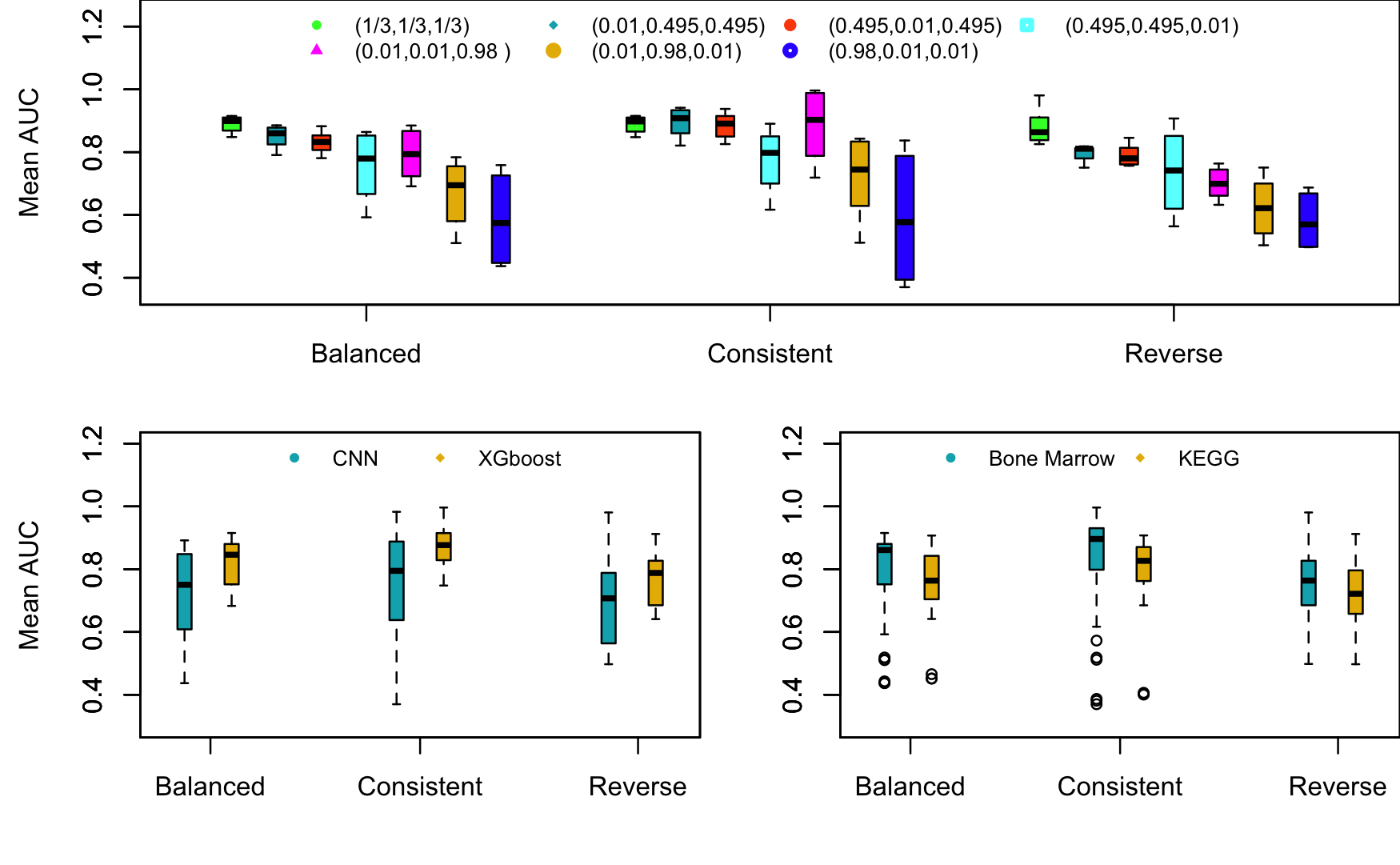
Figure 2: Boxplots of the mean AUC response under different levels of covariate variable and different combinations of label proportions for the three test scenarios.

For the boxplots of the mean AUC response under different combinations of label proportions, it is seen that under the label proportions are balanced (i.e., $(x_{1},x_{2},x_{3})=(1/3,1/3,1/3)$), the performance of mean AUC is usually better than those under other settings. It implies that the balance of class label proportions in the training dataset plays an important role for AI classification algorithms to achieve robustly good accuracy. When there are two classes dominating (e.g., $(x_{1},x_{2},x_{3})=(0.01,0.495,0.495)$), it is observed that the balance between class label 2 and label 3 ($x_{2}$ and $x_{3}$) gives better performance of mean AUC than the balance between class label 1 and label 2 ($x_{1}$ and $x_{2}$). When there is only one class dominating (e.g., $(x_{1},x_{2},x_{3})=(0.01,0.01,0.98)$), we observe that the performance under the class label 3 dominating is better than the performance under the class label 1 or label 2 dominating. This interesting pattern implies that the class label 3 plays a most substantial role among the three classes for the classification accuracy in terms of the mean AUC.

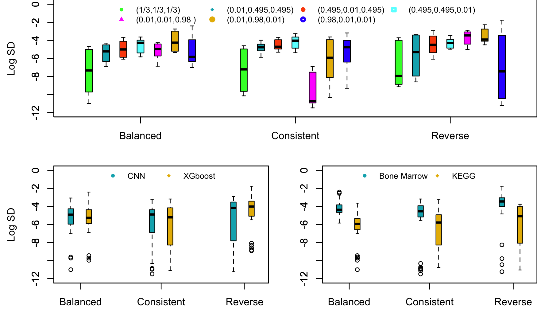
Figure 3: Boxplots of the Log SD response under different levels of covariate variable and different combinations of label proportions for the three test scenarios.

For the investigation of the Log SD as the response, note that a small value of Log SD means small variation of AUC values of three classes. That is, a smaller value of the Log SD is preferred. For covariate $z_{1}$, there is not a clear difference on Log SD between the CNN algorithm ($z_{1}=0$) and the XGboost algorithm ($z_{1}=1$). This implies that the two algorithms perform similarly with respect to the variation of AUC values from three classes. Under the Balanced Scenario of the test dataset, it is seen that the Log SD is more stable (i.e., narrow range on the boxplots) than those under the other two scenarios for covariate variable $z_{1}$. But for covariate variable $z_{2}$, the Log SD under the KEGG dataset ($z_{2}=0$) is generally smaller than the Log SD under the Bone Marrow dataset ($z_{2}=1$). In contrast to $z_{2}$ being not that significant for the mean AUC, the significance of $z_{2}$ for the Log SD implies that the KEGG dataset may provide more equally amount of information for three classes than the Bone Marrow dataset.

For the boxplots of the Log SD response under different combinations of label proportions, the general pattern is similar to the pattern for the boxplots of the mean AUC response. Specifically, the setting of balanced proportions of class label in the training dataset gives smaller Log SD than other settings. It indicates that the balance among class labels in the training dataset could help algorithms to obtain a small variation of the AUC values of three classes. When the proportions are dominated by two classes (e.g., $(x_{1},x_{2},x_{3})=(0.01,0.495,0.495)$), the setting gives slightly lower Log SD than the other two settings. The interesting patterns are observed when there is only one class prevailing. Under the Reverse Scenario, the range of Log SD for $(0.98,0.01,0.01)$ is the greatest, which may imply that such a setting could result in the most unstable classification performance. Under the Consistent Scenario, the Log SD for the setting $(0.01,0.01,0.98)$ is smallest even compared to the settings under the Balanced Scenario. One possible explanation is that when the class label 3 is dominating, the variation of AUC values for three classes becomes consistently low.

3.2 Modeling Results

In this section, we report analysis results of the regression model in Equation (2.3) for the mean AUC and the Log SD as the response, respectively. By fitting the regression model with the response of interest, we obtain estimated coefficients and their corresponding $t$-statistic and $p$-value. The prediction performance is also investigated for different class label proportions. The impact of predictor variables is assessed by the SHAP method.

Table 3: Parameter estimation and testing statistics under the Balanced Scenario.

Mean AUC Analysis					Log SD Analysis
Coef	Est	SE	$t$-value	$p$-value	Coef	Est	SE	$t$-value	$p$-value
$x_{1}$	0.4400	0.0173	25.440	$<$0.001	$x_{1}$	$-$4.631	0.565	$-$8.202	$<$0.001
$x_{2}$	0.5455	0.0173	31.546	$<$0.001	$x_{2}$	$-$2.714	0.565	$-$4.806	$<$0.001
$x_{3}$	0.8599	0.0173	49.764	$<$0.001	$x_{3}$	$-$3.937	0.565	$-$6.997	$<$0.001
$x_{1}x_{2}$	0.5989	0.0513	11.627	$<$0.001	$x_{1}x_{2}$	$-$3.228	1.677	$-$1.919	0.059
$x_{1}x_{3}$	0.6472	0.0513	12.604	$<$0.001	$x_{1}x_{3}$	$-$2.512	1.677	$-$1.498	0.139
$x_{2}x_{3}$	0.5512	0.0513	10.734	$<$0.001	$x_{2}x_{3}$	$-$6.725	1.677	$-$4.011	$<$0.001
$x_{1}z_{1}$	0.2532	0.0195	12.975	$<$0.001	$x_{1}z_{1}$	1.288	0.637	2.022	0.047
$x_{2}z_{1}$	0.1660	0.0195	8.506	$<$0.001	$x_{2}z_{1}$	$-$0.218	0.637	$-$0.343	0.733
$x_{3}z_{1}$	$-$0.0148	0.0195	$-$0.758	0.451	$x_{3}z_{1}$	0.179	0.637	0.281	0.779
$x_{1}z_{2}$	0.0241	0.0195	1.233	0.222	$x_{1}z_{2}$	$-$1.727	0.637	$-$2.711	0.008
$x_{2}z_{2}$	0.0744	0.0195	3.815	$<$0.001	$x_{2}z_{2}$	$-$1.721	0.637	$-$2.701	0.009
$x_{3}z_{2}$	$-$0.1186	0.0195	$-$6.088	$<$0.001	$x_{3}z_{2}$	$-$1.850	0.637	$-$2.909	0.005
$z_{1}z_{2}$	$-$0.0414	0.0160	$-$2.593	0.012	$z_{1}z_{2}$	$-$0.611	0.521	$-$1.172	0.245
Implied effect for $z_{1}$ and $z_{2}$
$z_{1}$	0.1348	0.0113	11.929	$<$0.001	$z_{1}$	0.416	0.369	1.127	0.263
$z_{2}$	$-$0.007	0.0113	$-$0.619	0.538	$z_{2}$	$-$1.766	0.369	$-$4.785	$<$0.001

Table 3 reports the analysis results for the Balanced Scenario. For the mean AUC, among significant factors with $p$-values less than $0.05$, the variable $x_{3}$ has the largest $t$ statistic. It confirms our observation from the data visualization that the class label 3 play a significant role in the classification accuracy. We also see that the estimated coefficients of interactions between two proportions (i.e. $x_{j}x_{j^{\prime}}$’s) are all positive. It implies that balance in the training dataset will increase the accuracy of the classification algorithms. For covariate variable $z_{1}$ concerning two algorithms, the estimated coefficient of $z_{1}$ is positive with a statistically significant effect. It confirms that the XGboost algorithm produces a higher mean AUC in comparison with the CNN algorithm. For covariate variable $z_{2}$ concerning the two datasets (i.e., the KEGG and the Bone Marrow datasets), the corresponding $p$-value is $0.538>0.05$, which confirms data visualization that $z_{2}$ does not provide significantly influence on the Mean AUC.

For the Log SD analysis, only the main effects of proportions and several interaction effects are statistically significant. It is seen that covariate $z_{1}$ does not have a significant effect for the Log SD, which is consistent with the data visualization. Note that $x_{2}x_{3}$ is significant with the largest $t$-statistic, which may imply that the proportions of $x_{2}$ and $x_{3}$ are essential to minimize the dispersion of the AUC values among three classes.

Table 4: Parameter estimation and testing statistics under the Consistent Scenario.

Mean AUC Analysis					Log SD Analysis
Coef	Est	SE	$t$-value	$p$-value	Coef	Est	SE	$t$-value	$p$-value
$x_{1}$	0.4122	0.0273	17.386	$<$0.001	$x_{1}$	$-$3.649	0.836	$-$4.367	$<$0.001
$x_{2}$	0.5833	0.0273	24.604	$<$0.001	$x_{2}$	$-$5.523	0.836	$-$6.608	$<$0.001
$x_{3}$	1.0009	0.0273	42.251	$<$0.001	$x_{3}$	$-$10.448	0.836	$-$12.511	$<$0.001
$x_{1}x_{2}$	0.5091	0.0704	7.210	$<$0.001	$x_{1}x_{2}$	1.514	2.481	0.608	0.545
$x_{1}x_{3}$	0.6150	0.0704	8.737	$<$0.001	$x_{1}x_{3}$	7.079	2.481	2.853	0.006
$x_{2}x_{3}$	0.3838	0.0704	5.453	$<$0.001	$x_{2}x_{3}$	7.823	2.481	3.153	0.002
$x_{1}z_{1}$	0.3068	0.0267	11.471	$<$0.001	$x_{1}z_{1}$	$-$0.102	0.943	$-$0.109	0.914
$x_{2}z_{1}$	0.1576	0.0267	5.894	$<$0.001	$x_{2}z_{1}$	1.185	0.943	1.257	0.213
$x_{3}z_{1}$	$-$0.0366	0.0267	$-$1.371	0.175	$x_{3}z_{1}$	0.428	0.943	0.455	0.651
$x_{1}z_{2}$	0.0290	0.0267	1.083	0.282	$x_{1}z_{2}$	$-$1.922	0.943	$-$2.038	0.045
$x_{2}z_{2}$	0.1085	0.0267	4.058	$<$0.001	$x_{2}z_{2}$	$-$1.283	0.943	$-1.361$	0.178
$x_{3}z_{2}$	$-$0.1943	0.0267	$-$7.273	$<$0.001	$x_{3}z_{2}$	2.498	0.943	2.653	0.010
$z_{1}z_{2}$	$-$0.0189	0.0219	$-$0.861	0.392	$z_{1}z_{2}$	$-$2.002	0.772	$-$2.594	0.012
Implied effect for $z_{1}$ and $z_{2}$
$z_{1}$	0.1426	0.0155	9.200	$<$0.001	$z_{1}$	0.504	0.546	0.923	0.359
$z_{2}$	$-$0.0189	0.0155	$-$1.219	0.227	$z_{2}$	$-$0.236	0.546	$-$0.432	0.667

Table 4 reports the analysis results for the Consistent Scenario. It is seen that almost all terms involving the class proportion $x_{3}$ are significant for both mean AUC and Log SD. This implies that the proportion of class label 3 is not only of most importance to maintain the classification accuracy, but also important for the variation of the AUC values of the three classes. The covariate variable $z_{1}$ is significant with a positive coefficient, indicating that the XGboost algorithm performs better than the CNN algorithm for the mean AUC in the Consistent Scenario. For the Log SD, the estimated coefficient for $x_{1}x_{3}$, which is not significant in the Balanced Scenario, becomes statistically significant. A possible explanation is that the proportion of label 1 becomes more important in the Consistent Scenario than that in the Balanced Scenario. Under the Consistent Scenario, the results in Table 4 show that both covariates $z_{1}$ and $z_{2}$ seem not having much influence on the Log SD.

Table 5: Parameter estimation and testing statistics under the Reverse Scenario.

Mean AUC Analysis					Log SD Analysis
Coef	Est	SE	$t$-value	$p$-value	Coef	Est	SE	$t$-value	$p$-value
$x_{1}$	0.4755	0.0205	23.245	$<$0.001	$x_{1}$	$-$8.713	0.716	$-$12.162	$<$0.001
$x_{2}$	0.5211	0.0205	25.472	$<$0.001	$x_{2}$	$-$2.181	0.716	$-$3.044	0.003
$x_{3}$	0.7350	0.0205	35.960	$<$0.001	$x_{3}$	$-$1.873	0.716	$-$2.617	0.011
$x_{1}x_{2}$	0.6454	0.0607	10.594	$<$0.001	$x_{1}x_{2}$	1.594	2.127	0.747	0.458
$x_{1}x_{3}$	0.6990	0.0607	11.509	$<$0.001	$x_{1}x_{3}$	1.303	2.127	0.613	0.542
$x_{2}x_{3}$	0.6472	0.0607	10.656	$<$0.001	$x_{2}x_{3}$	$-$11.262	2.127	$-$5.295	$<$0.001
$x_{1}z_{1}$	0.1807	0.0231	7.831	$<$0.001	$x_{1}z_{1}$	4.950	0.808	6.125	$<$0.001
$x_{2}z_{1}$	0.1737	0.0231	7.524	$<$0.001	$x_{2}z_{1}$	$-$0.463	0.808	$-$0.573	0.568
$x_{3}z_{1}$	$-$0.0208	0.0231	$-$0.901	0.371	$x_{3}z_{1}$	$-$0.233	0.808	$-$0.288	0.774
$x_{1}z_{2}$	0.0105	0.0231	0.456	0.650	$x_{1}z_{2}$	$-$1.132	0.808	$-$1.400	0.166
$x_{2}z_{2}$	0.0150	0.0231	0.650	0.517	$x_{2}z_{2}$	$-$1.449	0.808	$-$1.792	0.077
$x_{3}z_{2}$	$-$0.0576	0.0231	$-$2.500	0.015	$x_{3}z_{2}$	$-$2.635	0.808	$-$3.265	0.002
$z_{1}z_{2}$	$-$0.0319	0.0189	$-$1.688	0.096	$z_{1}z_{2}$	$-$0.695	0.661	$-$1.051	0.297
Implied effect for $z_{1}$ and $z_{2}$
$z_{1}$	0.1112	0.0114	9.754	$<$0.001	$z_{1}$	1.418	0.468	3.030	0.003
$z_{2}$	$-$0.012	0.0114	$-$1.053	0.296	$z_{2}$	$-$1.739	0.468	$-$3.716	$<$0.001

Table 5 reports the analysis results for the Reverse Scenario. The significance of $x_{3}$ (i.e., the proportion of class 3) has the similar pattern as what we observed in both the balanced scenario and the consistent scenario. The covariate $z_{1}$ is significant for the mean AUC, but it is not significant for the Log SD. In contrast, covariate $z_{2}$ is significant for the log SD, but it is not significant for the mean AUC. It is interesting to note that, under the Reverse Scenario, the $t$-statistic for $x_{1}$ is the largest in absolute value for the Log SD. It may indicate that the proportion of label 1 becomes crucial to affect the variation of AUC values among three classes in the Reverse Scenario.

Furthermore, we evaluate the performance of the estimated model at different proportions of class labels $(x_{1},x_{2},x_{3})$. Specifically, given a level combination of covariate variables $z_{1}$ and $z_{2}$, we provide the triangle contour plots of prediction at $(x_{1},x_{2},x_{3})$. Figure 4 shows the triangle contour plots of prediction for the Mean AUC under different level combinations of the covariate variables. Based those results in Figure 4, the prediction accuracy of the classification algorithms (i.e., the predicted mean AUC) generally achieves the best performance when the class proportions are balanced (i.e., $(x_{1},x_{2},x_{3}=(1/3,1/3,1/3)$). However, comparing the XGboost ($z_{1}=1$) and the CNN ($z_{1}=0$), the XGboost algorithm appears to be more symmetric with respect to three vertex $x_{1}$, $x_{2}$, and $x_{3}$. While the prediction accuracy of the CNN algorithm appears to be more affected by the proportion of the class 3. It is noted that, under the setting of the Consistent Scenario, both classification algorithms can achieve the perfect accuracy (i.e., prediction of the mean AUC being 1) under the setting of class proportion $x_{3}$ prevailing. One plausible explanation is that data points from class 3 are more important than the data points from the other two classes in terms of affecting the classification accuracy for the KEGG and the Bone Marrow datasets in this study.

Figure 4 shows the triangle contour plots of prediction for the Log SD under different level combinations of the covariate variables. The patterns of the contour plots are generally more heterogeneous across different level combinations of covariate variables $z_{1}$ and $z_{2}$. One interesting observation is that the prediction pattern in the contour plot is not symmetric with respect to three vertex $x_{1}$, $x_{2}$, and $x_{3}$. It may imply that the data points from the three classes do not equally contribute to the classification performance in terms of the variation of the AUC values from three classes.

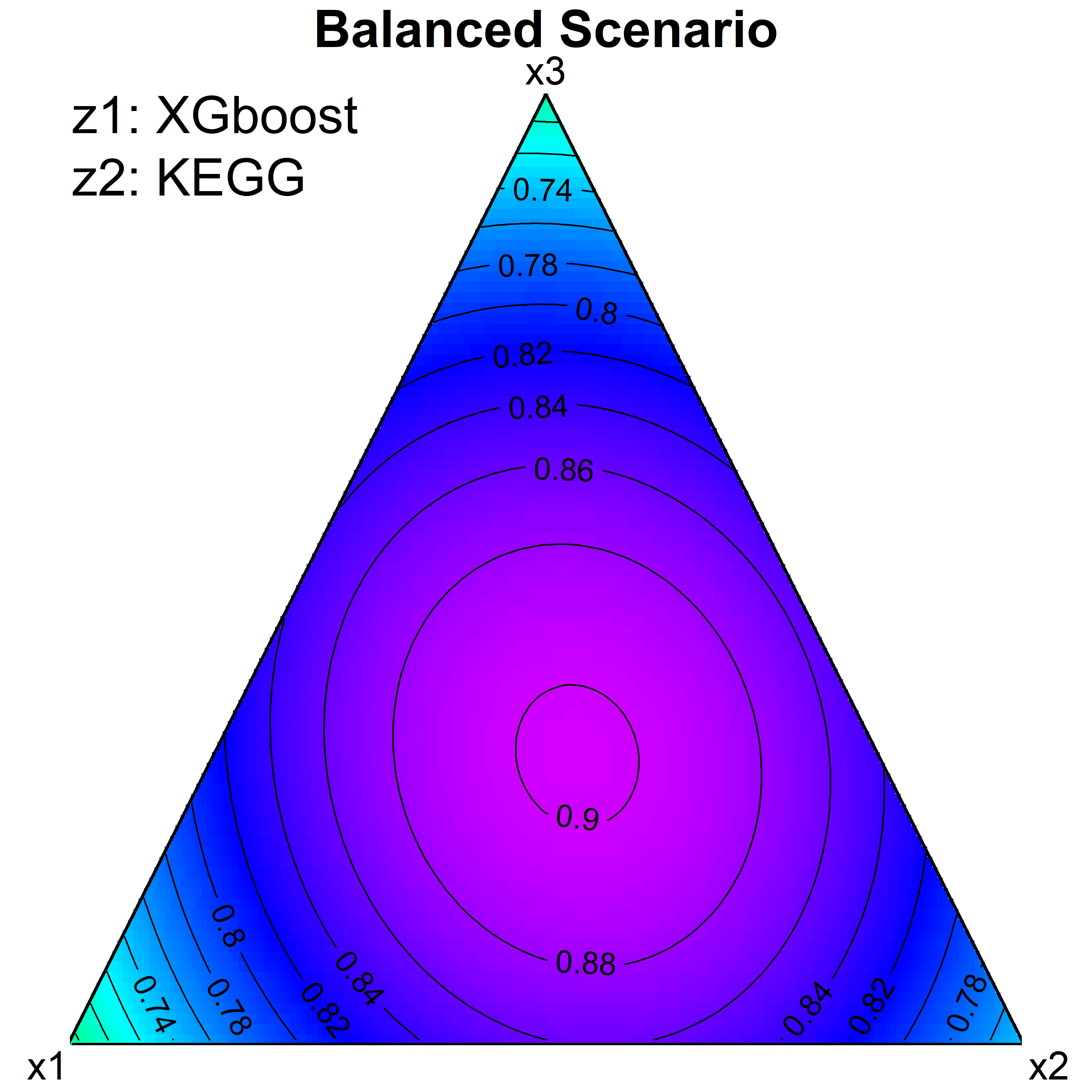
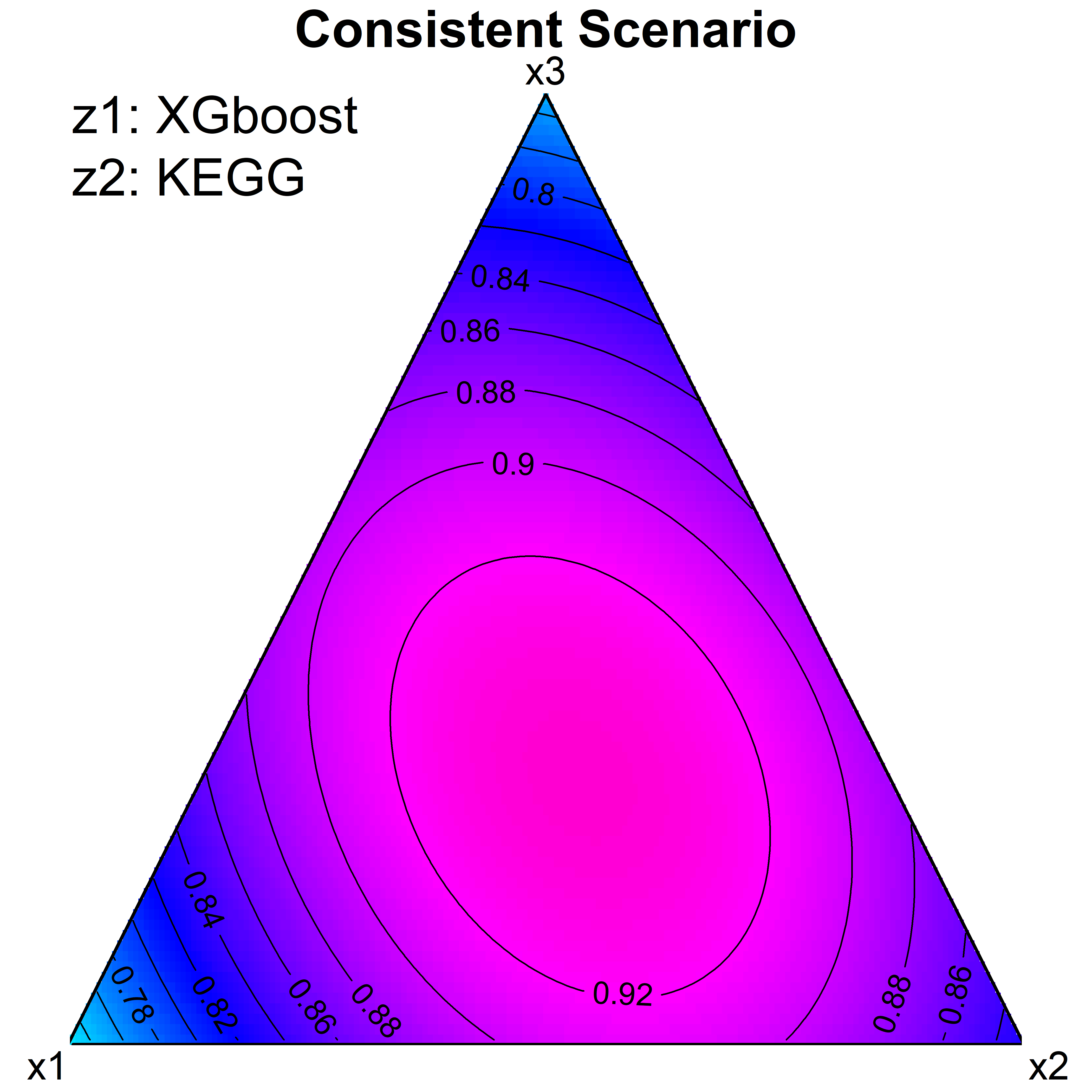
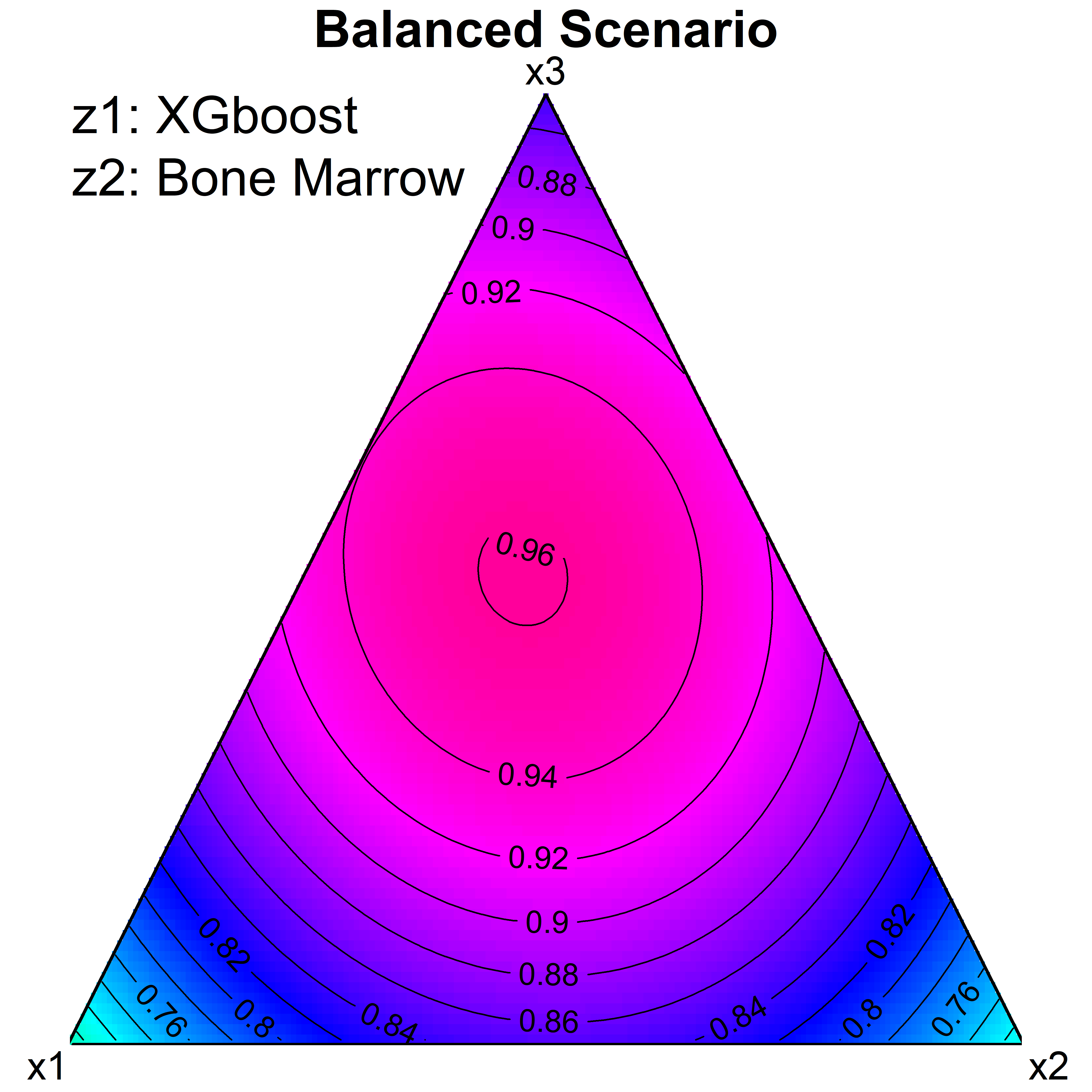
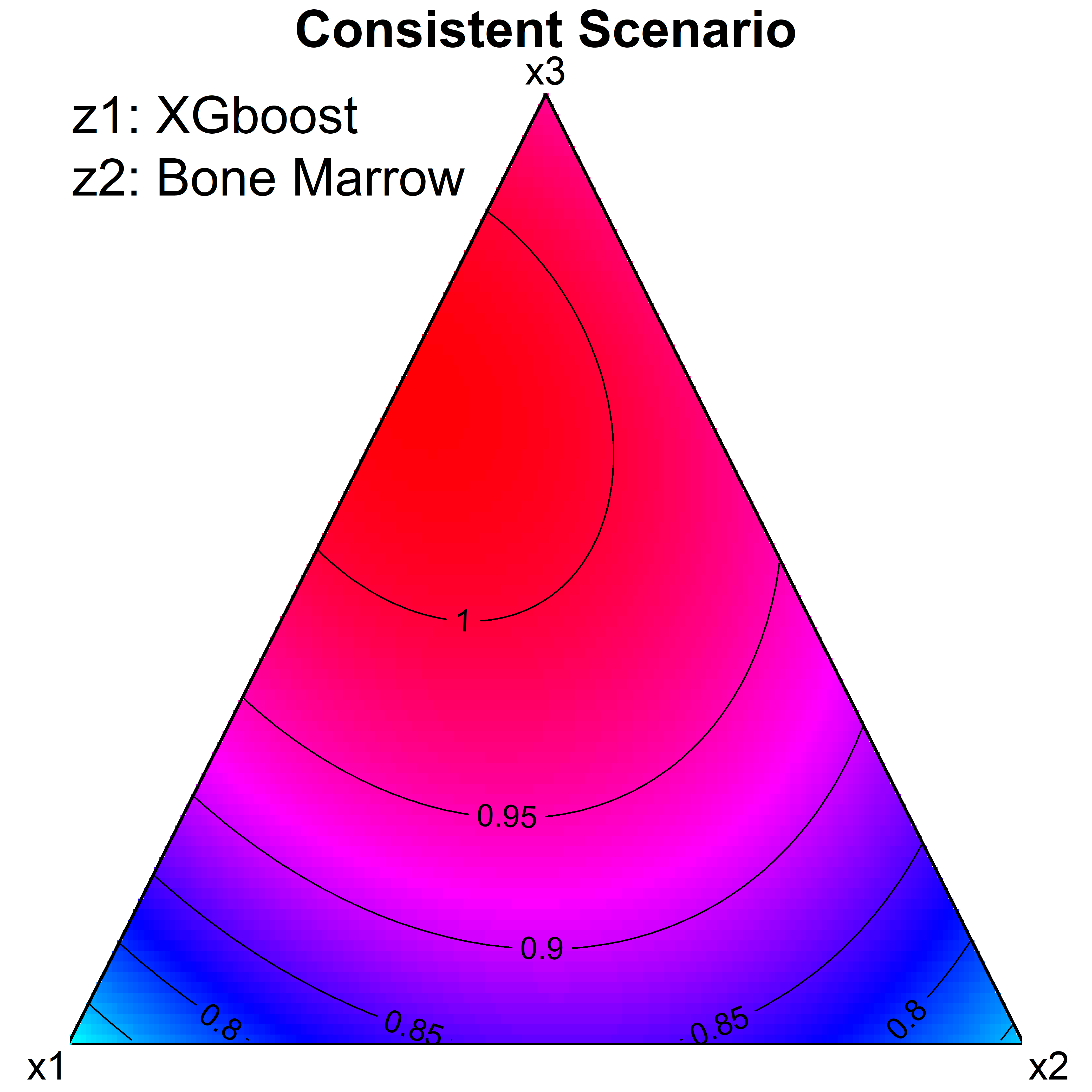
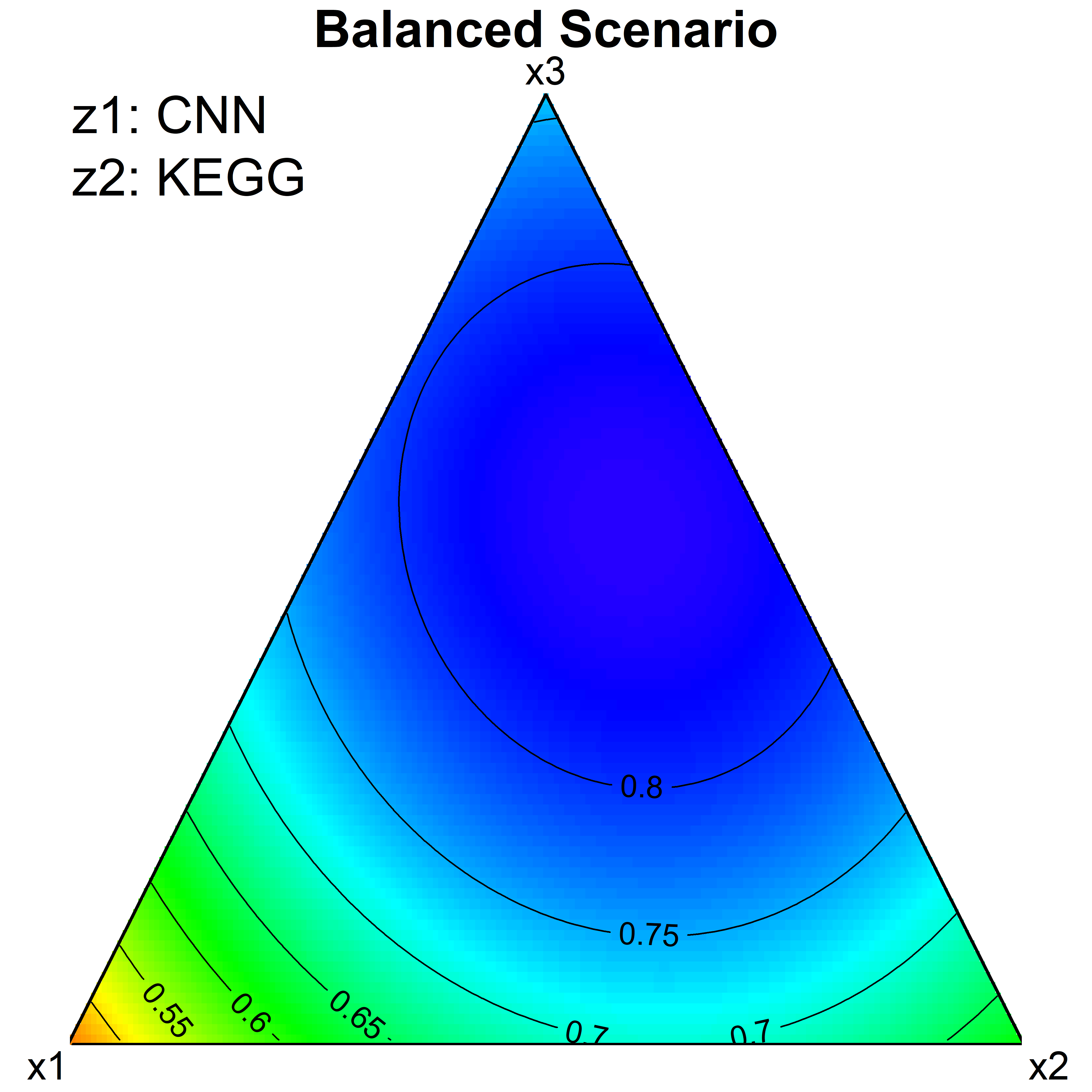
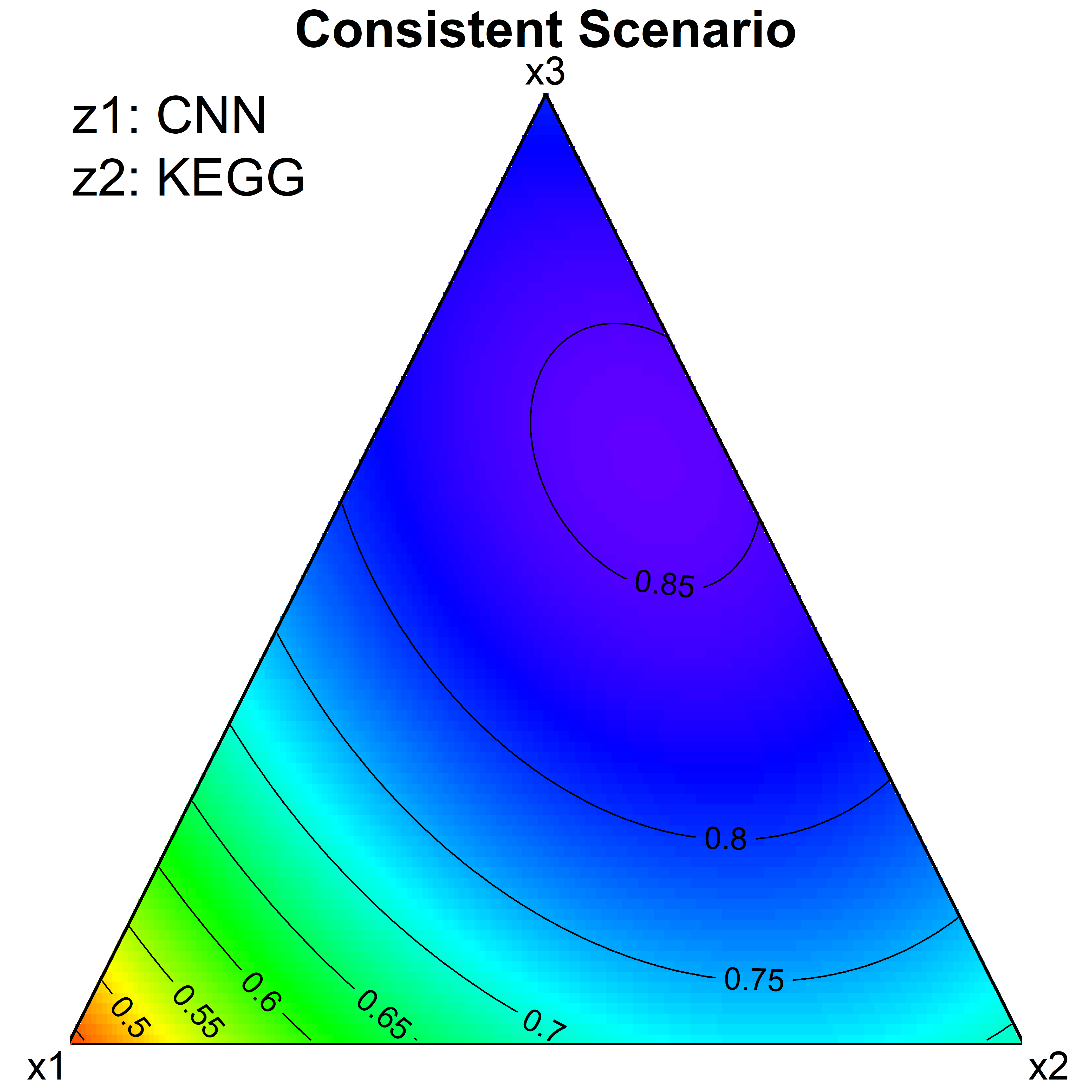
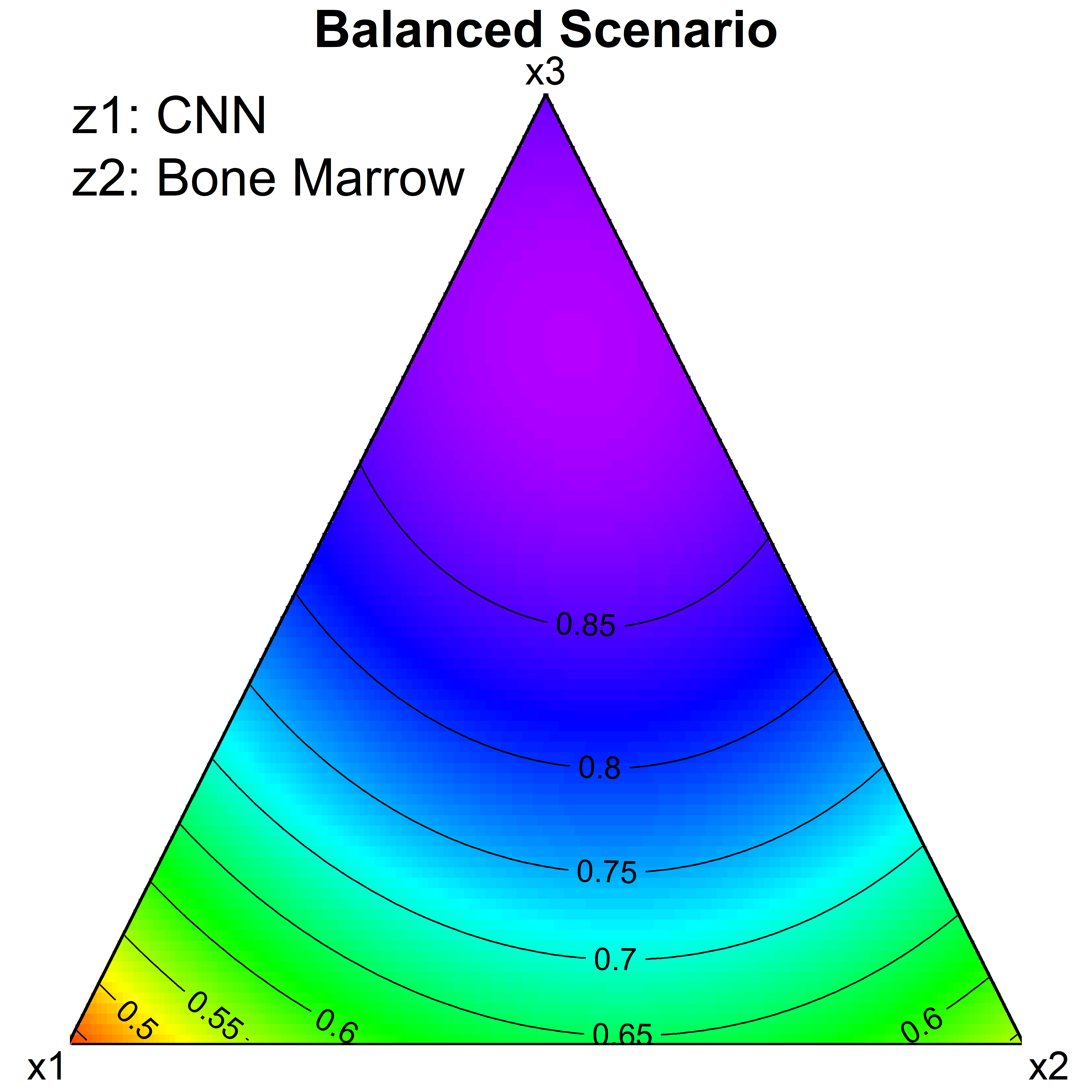
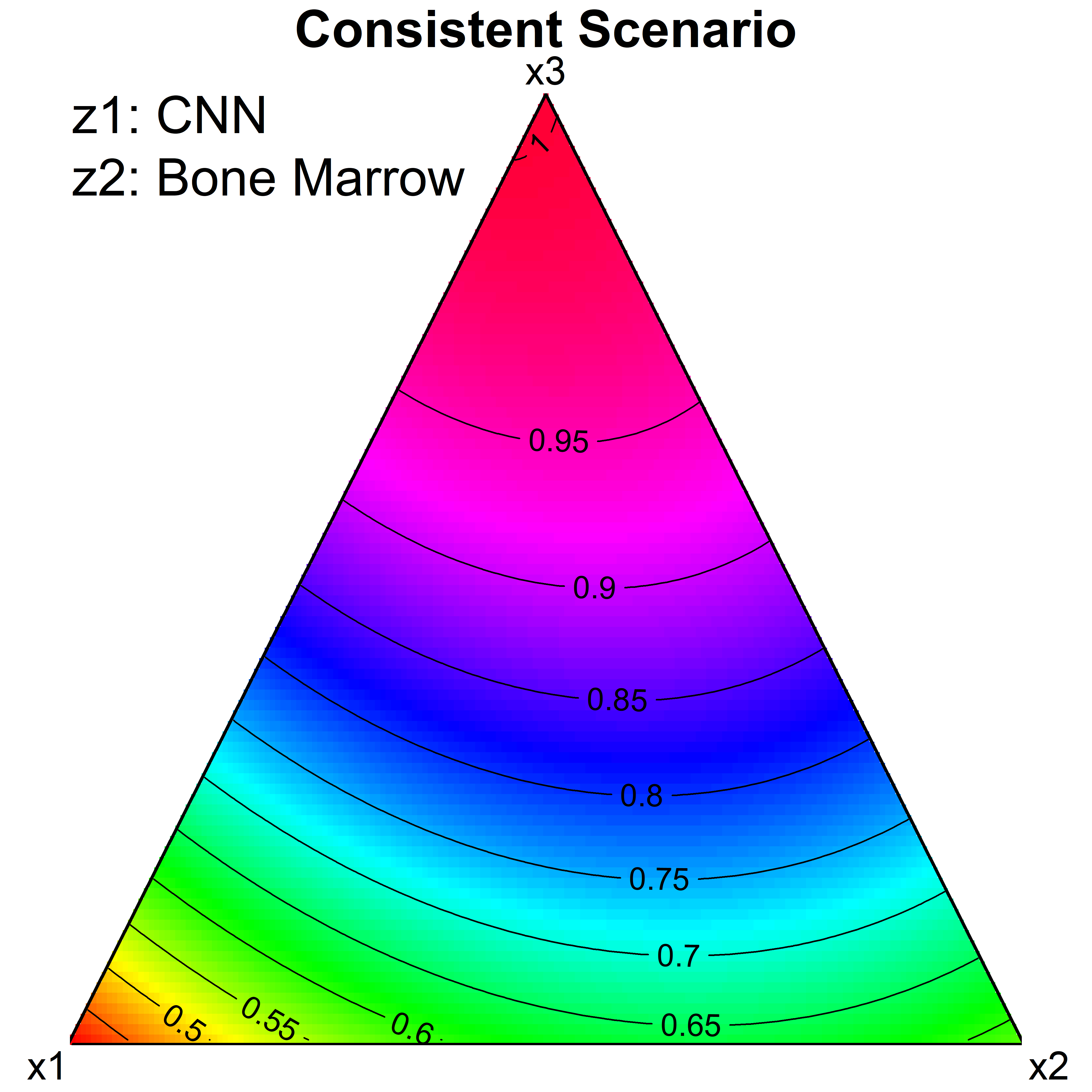
Figure 4: The triangle contour plots of prediction for the Mean AUC under three scenarios.

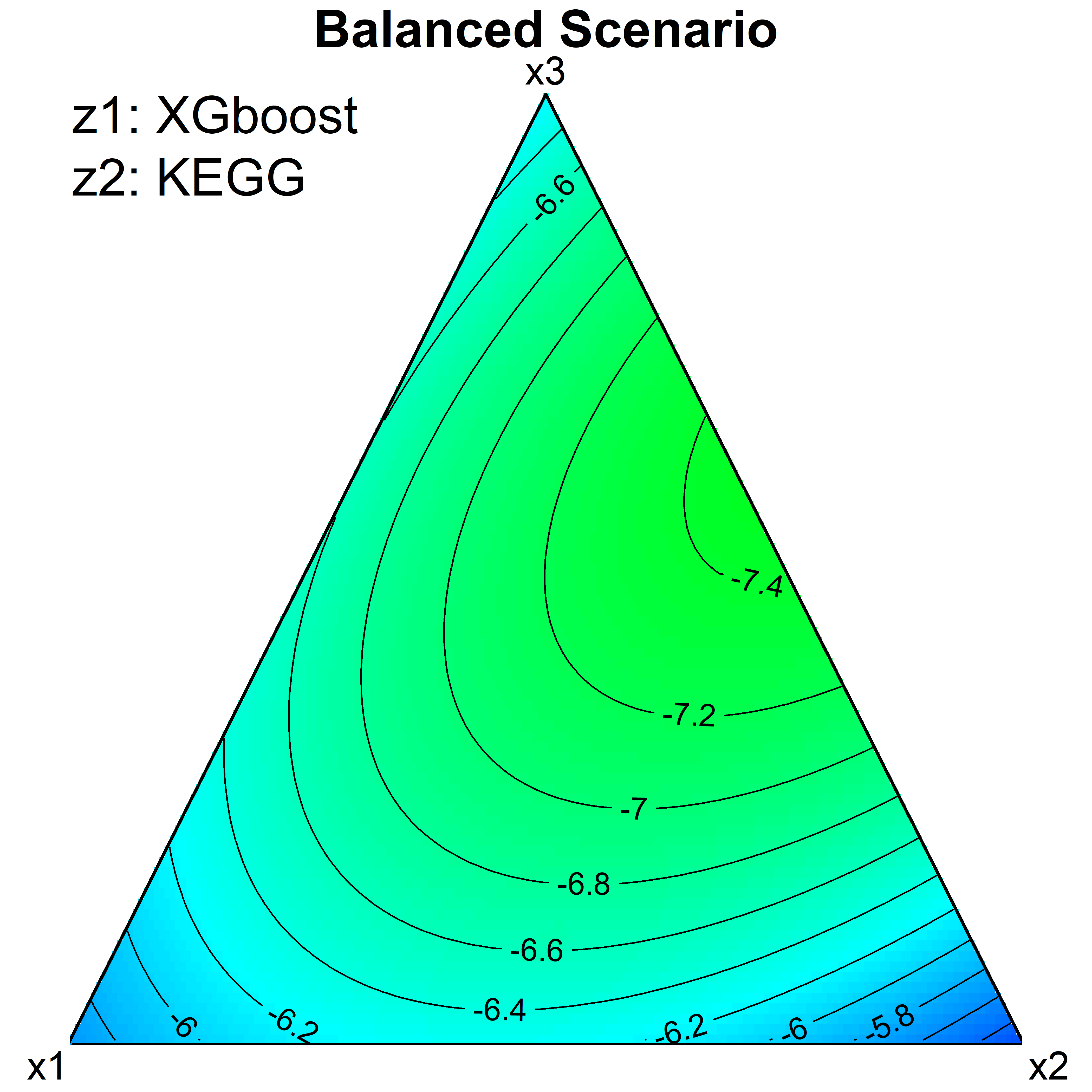
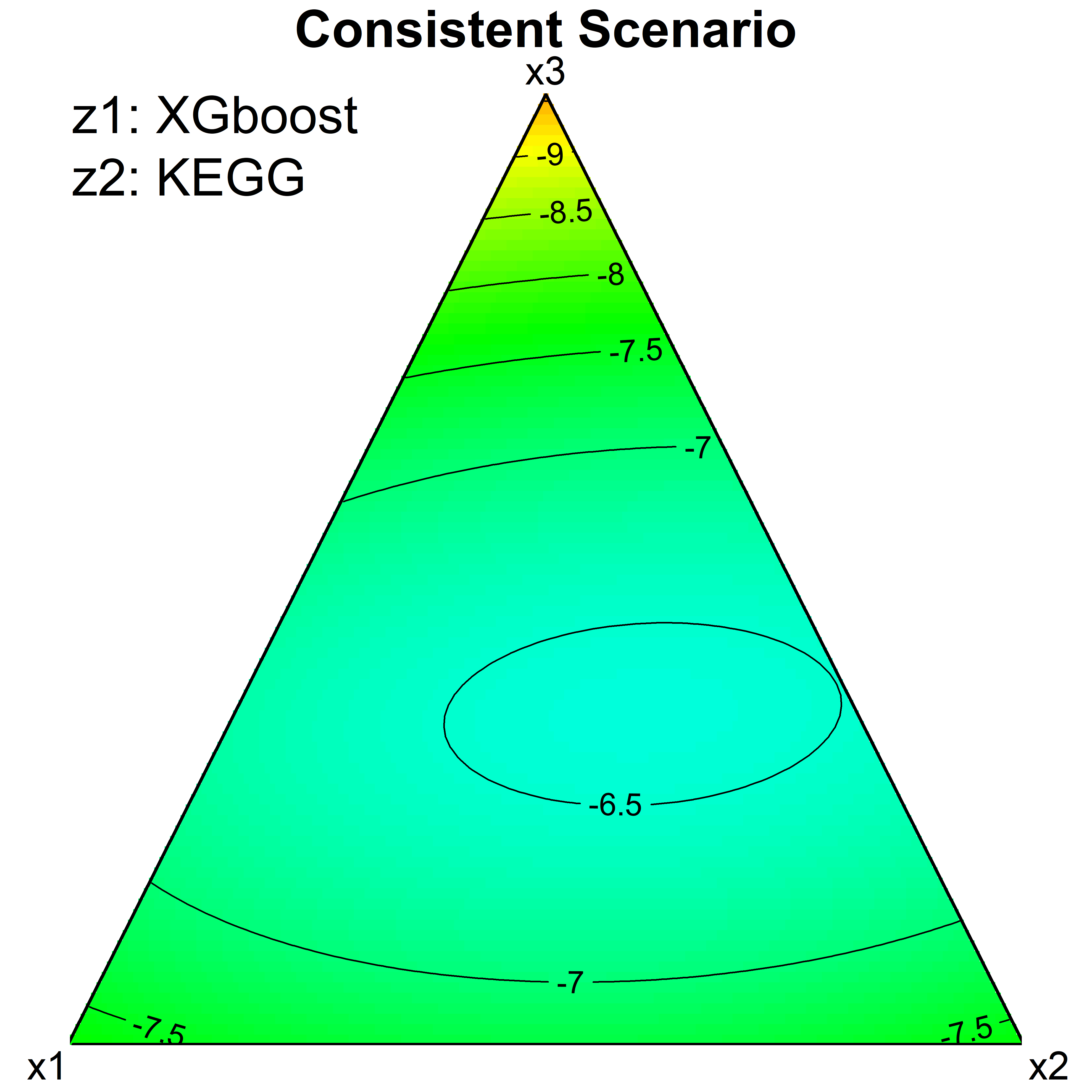
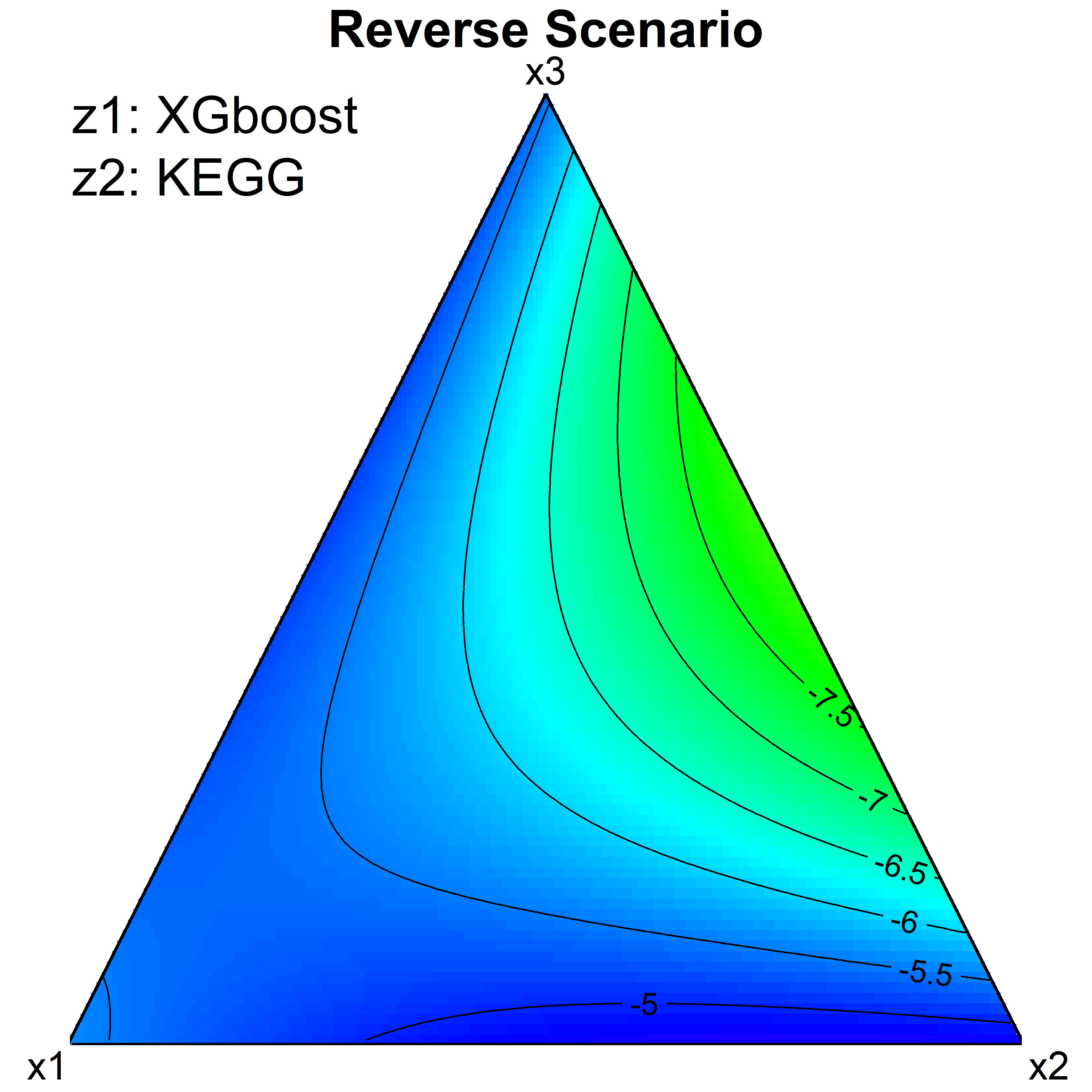
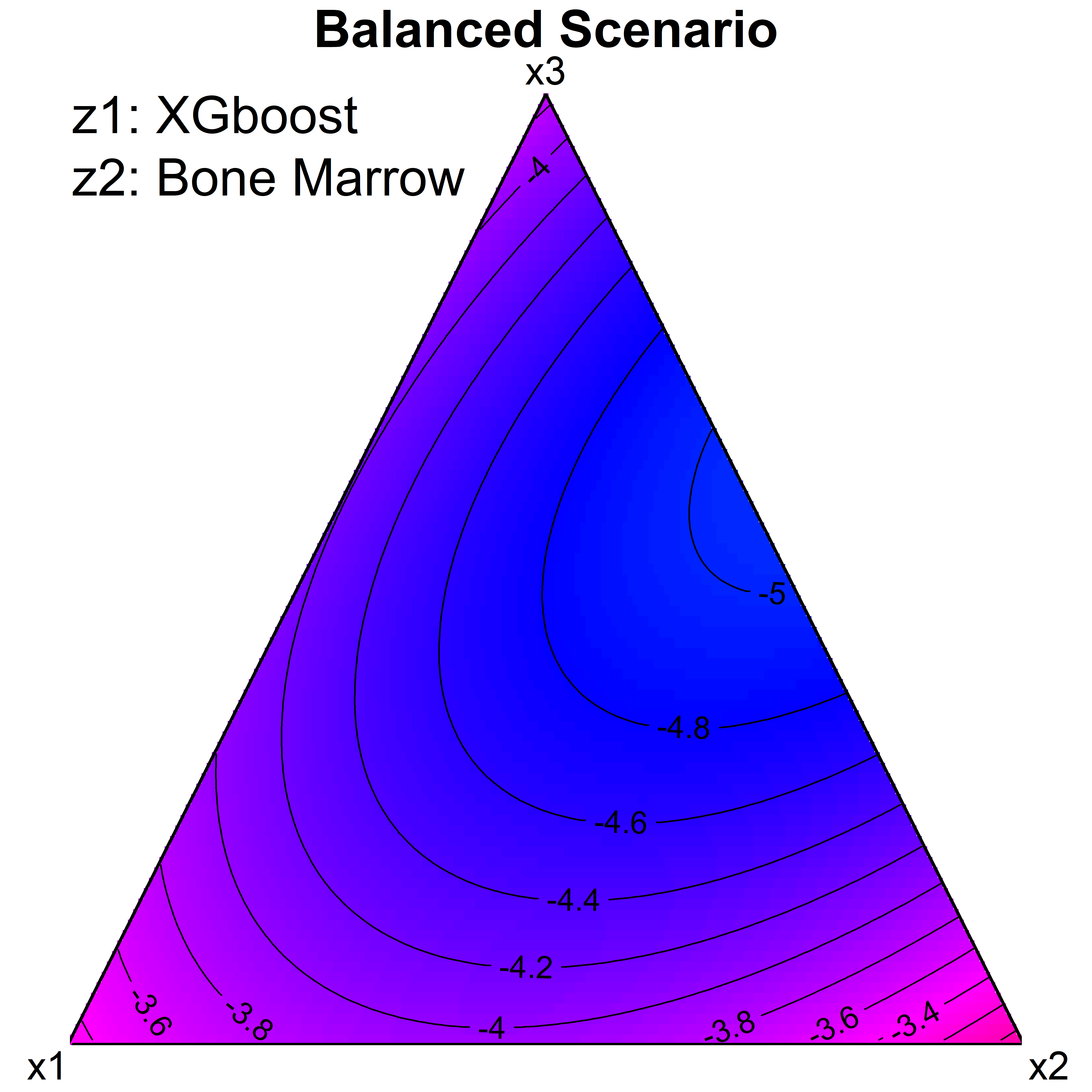
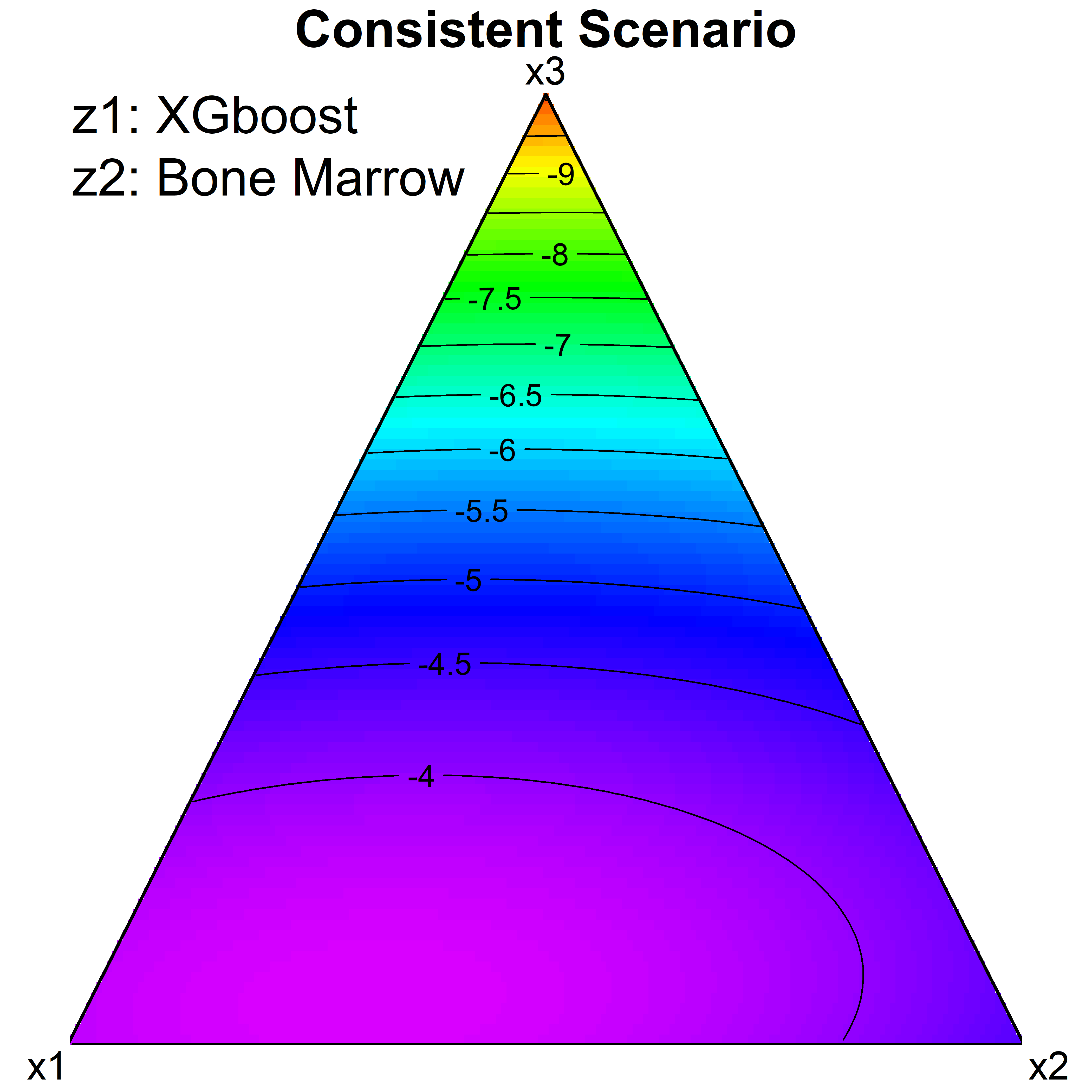
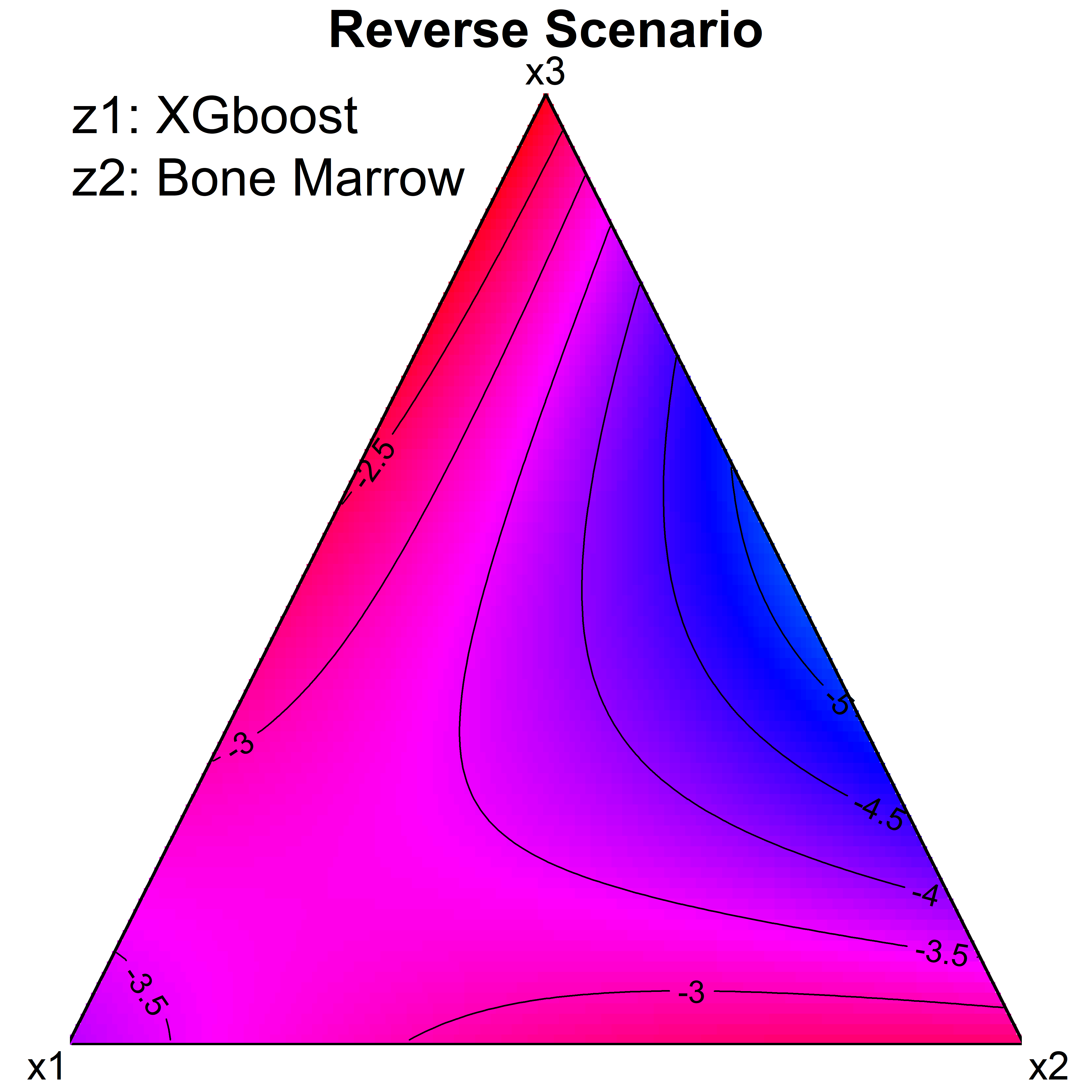
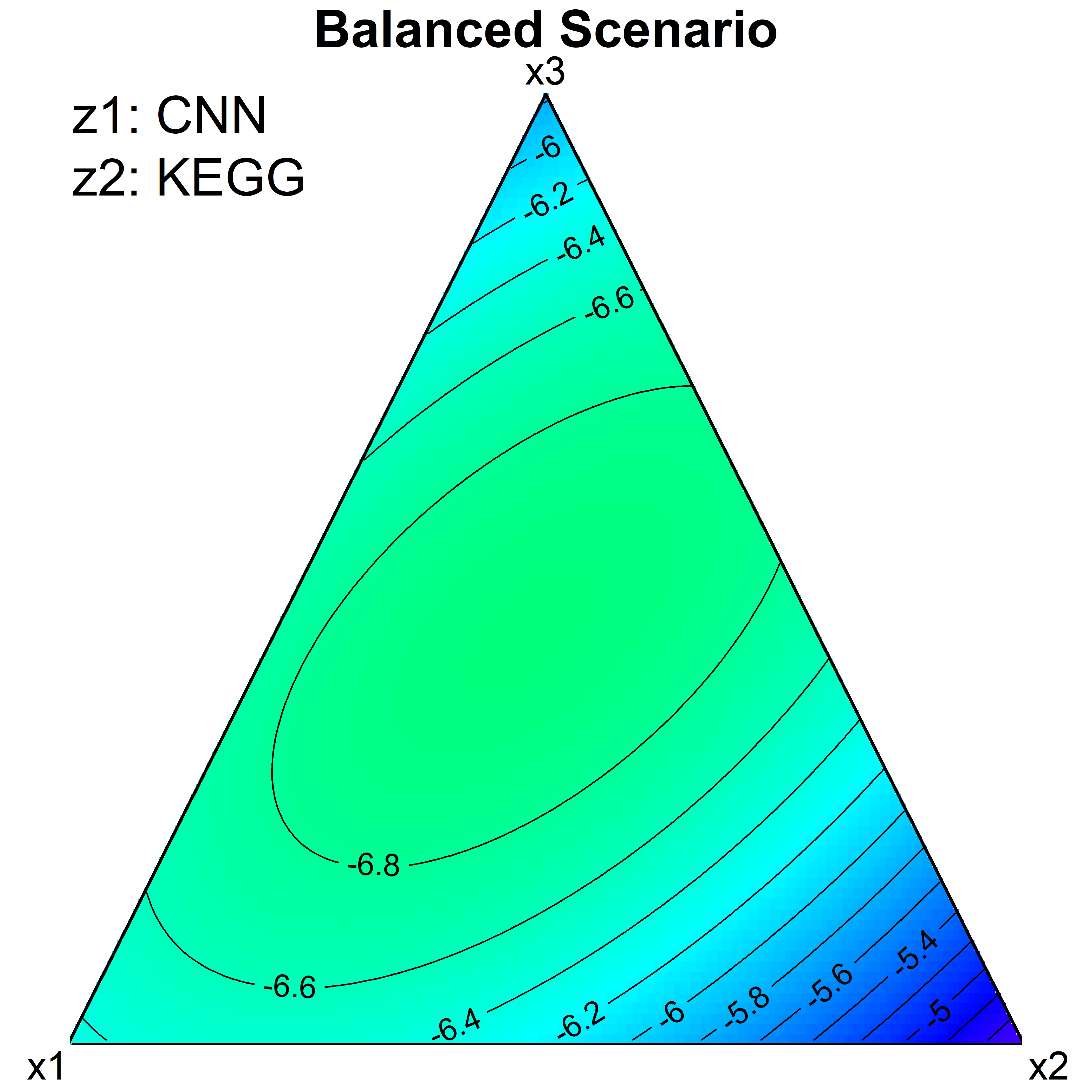
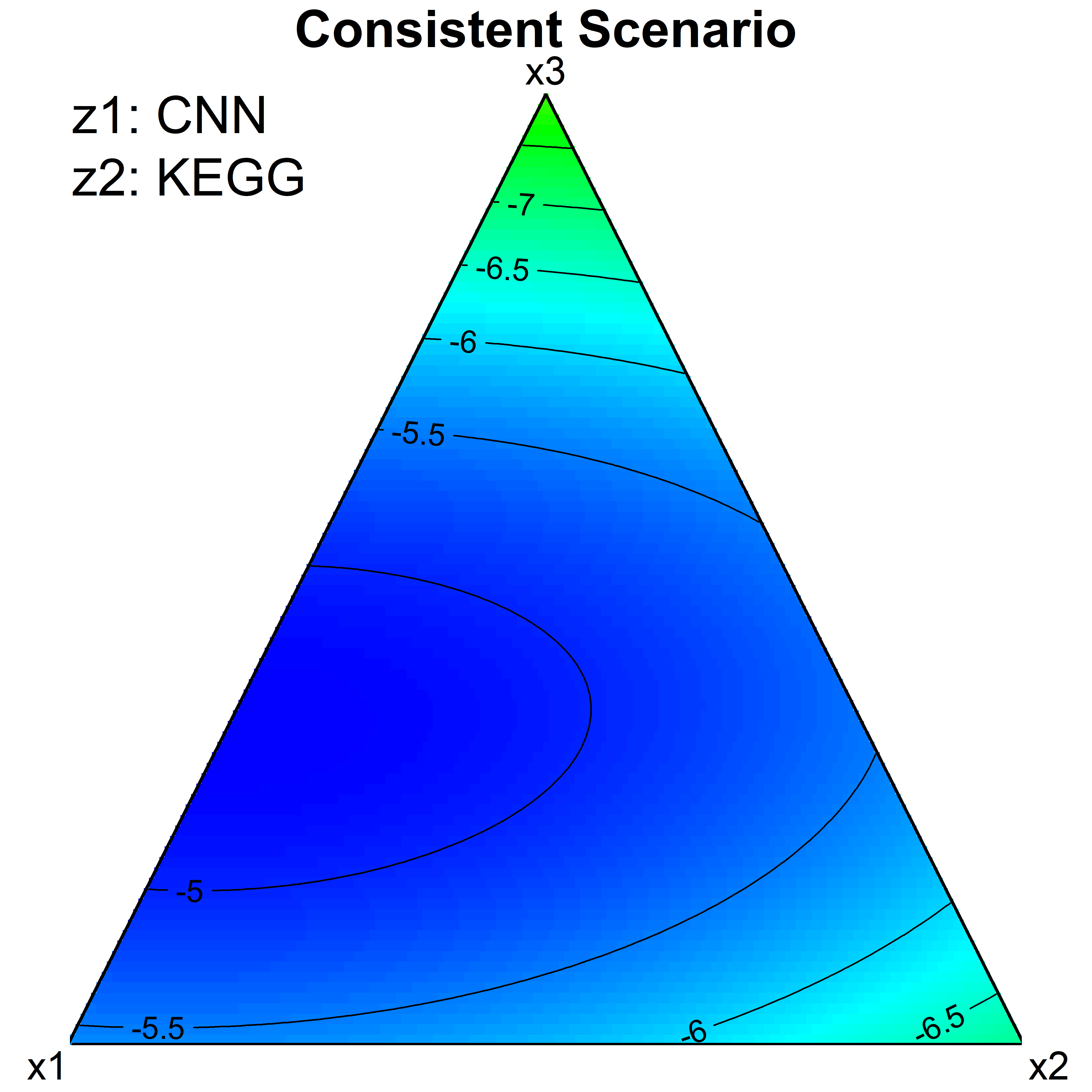
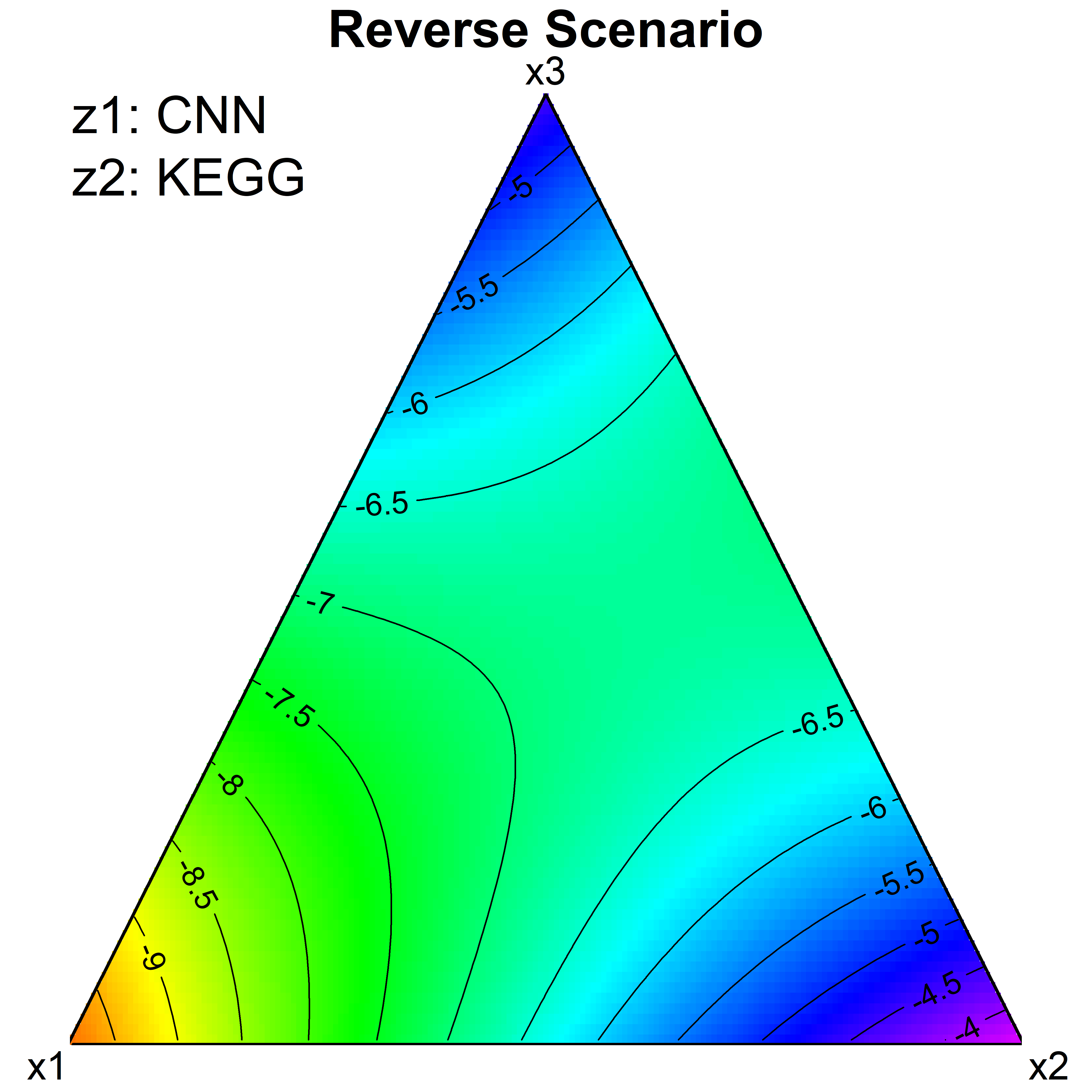
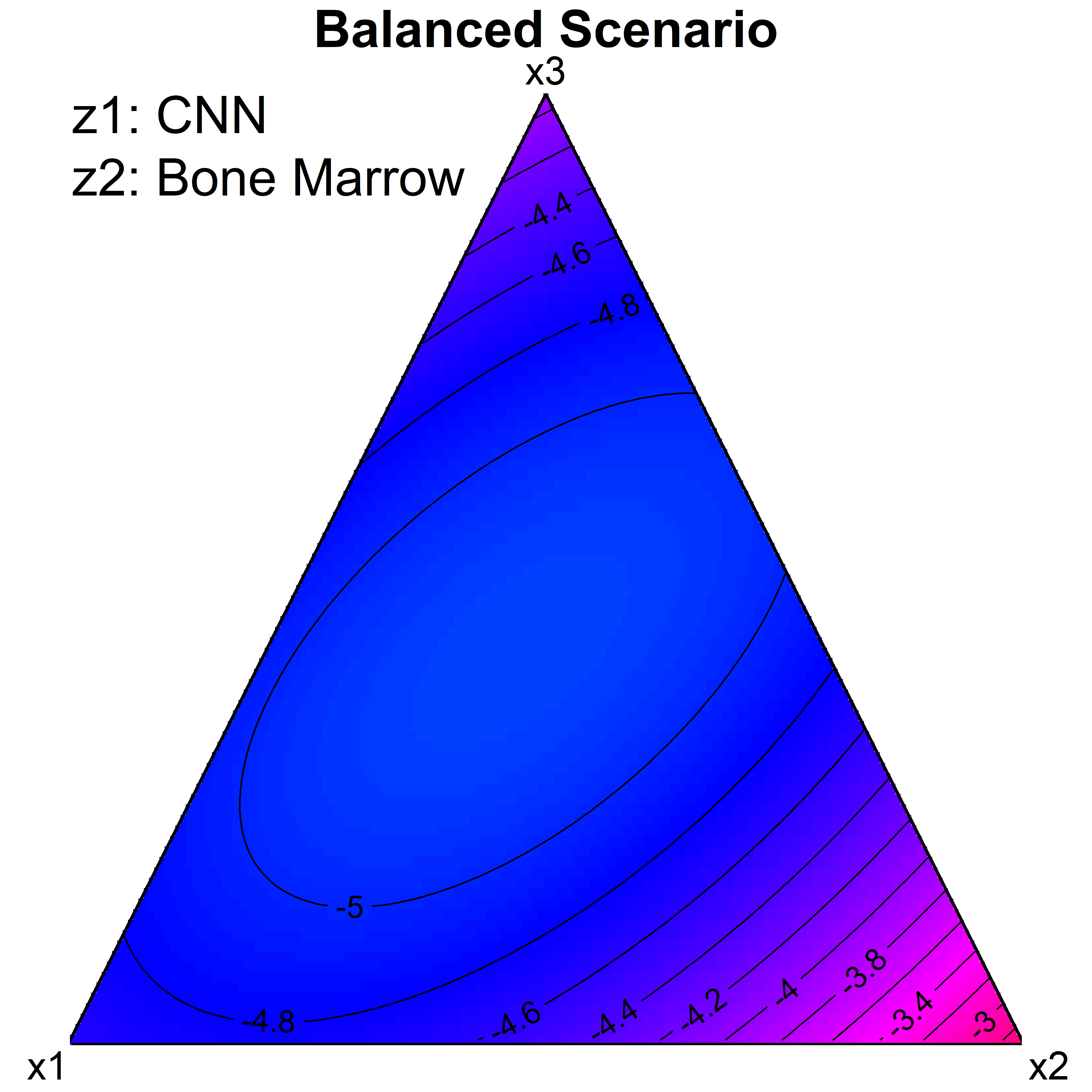
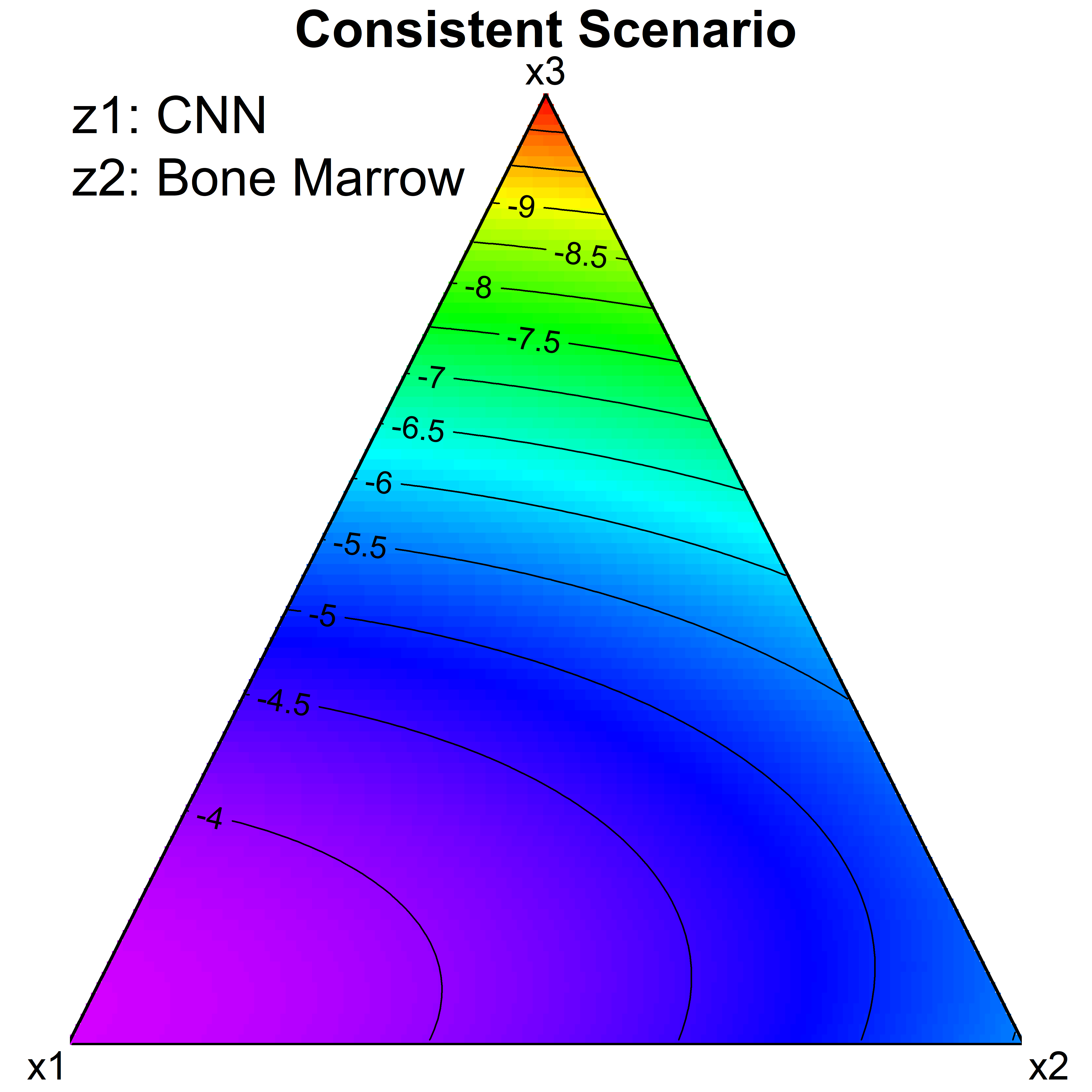
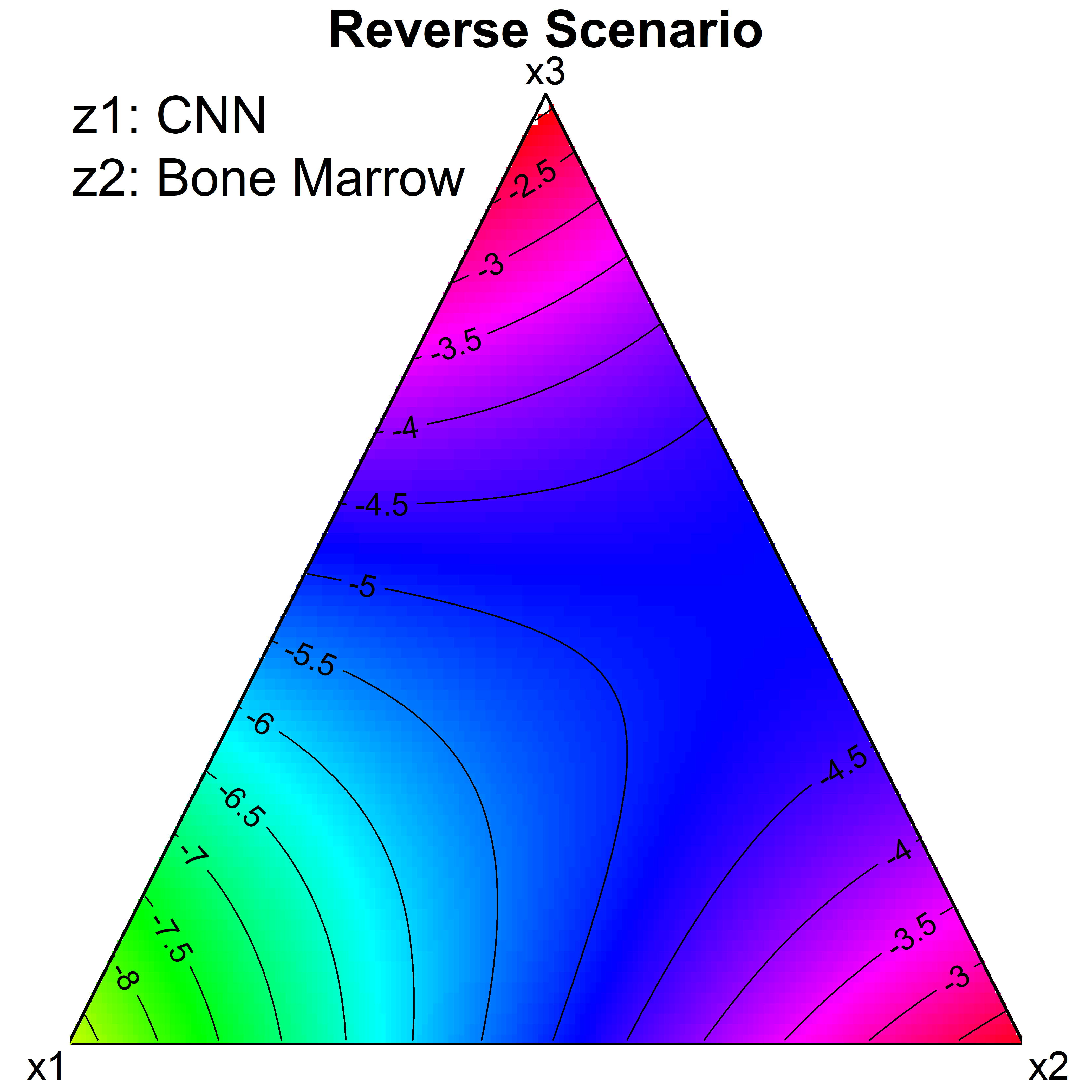
Figure 5: The triangle contour plots of prediction for the Log SD under the three scenarios.

Lastly, we examine the impact of predictor variables to the response through the Shapely values in (3)-(6). Table 6 reports the Shapley values of predictor variables in the estimated models for the mean AUC and the Log SD, respectively. From the results in the table, it is clear that the proportion of class label 3, $x_{3}$, has the largest impact on the mean AUC for all the three scenarios. While for the Log SD, the proportion of class label 1, $x_{1}$, has the largest impact to the response under the Reverse and Balanced Scenarios, and the proportion of class label 3, $x_{3}$, has the largest impact to the response under the Consistent Scenario.

Table 6: The Shapley values of predictor variables in the estimated model for the mean AUC and the Log SD under the three scenarios.

Mean AUC Analysis				Log SD Analysis
Coef	Balanced	Consistent	Reverse	Coef	Balanced	Consistent	Reverse
$x_{1}$	0.118	0.110	0.127	$x_{1}$	1.239	0.977	2.332
$x_{2}$	0.151	0.162	0.145	$x_{2}$	0.753	1.533	0.605
$x_{3}$	0.250	0.291	0.213	$x_{3}$	1.143	3.033	0.544
$x_{1}x_{2}$	0.042	0.036	0.045	$x_{1}x_{2}$	0.226	0.106	0.112
$x_{1}x_{3}$	0.046	0.043	0.049	$x_{1}x_{3}$	0.177	0.499	0.092
$x_{2}x_{3}$	0.039	0.027	0.045	$x_{2}x_{3}$	0.473	0.550	0.792
$x_{1}z_{1}$	0.059	0.072	0.042	$x_{1}z_{1}$	0.301	0.024	1.156
$x_{2}z_{1}$	0.039	0.037	0.041	$x_{2}z_{1}$	0.051	0.277	0.108
$x_{3}z_{1}$	0.003	0.009	0.005	$x_{3}z_{1}$	0.042	0.100	0.055
$x_{1}z_{2}$	0.006	0.007	0.002	$x_{1}z_{2}$	0.403	0.449	0.264
$x_{2}z_{2}$	0.017	0.025	0.004	$x_{2}z_{2}$	0.402	0.300	0.338
$x_{3}z_{2}$	0.028	0.046	0.014	$x_{3}z_{2}$	0.434	0.586	0.618
$z_{1}z_{2}$	0.016	0.007	0.012	$z_{1}z_{2}$	0.229	0.751	0.261

3.3 Summary of Findings

Based on the data visualization in Section 3.1 and the modeling results in Section 3.2, we provide a summary of the findings as follows.

• The balanced setting of the class label proportions generally gives the best classification accuracy in terms of the mean AUC for all the three test scenarios. This finding is applicable for both the CNN and XGboost algorithms. • The proportions of class labels may not be of equal importance for the robustness of the AI algorithms. For the KEGG and Bone Marrow datasets studied in this paper, the proportion of class label 3 in the training data appears to be more important than the other two class labels for classification accuracy in terms of the mean AUC. • The choice of classification algorithms (i.e., covariate variable $z_{1}$) appears to have a statistically significant effect on the response of the mean AUC, but may not be significant for the Log SD, which measures the variation of the AUC values of $m$ classes. • The interactions between the class label proportions and the chosen algorithm are often significant for the classification performance in terms of the mean AUC and the Log SD. • The predicted mean AUC based on the proposed model generally achieves the largest accuracy under the setting of class proportions being balanced in the training dataset. • For the response Log SD, the patterns of significant factors and predicted values are generally more heterogeneous across different level combinations of the covariate variables.

4 Concluding Remarks

In this work, we propose an experimental design framework to systematically investigate the robustness of the AI classification algorithms. In particular, we adopt the idea of mixture experiments to investigate how the proportion of class labels in the training dataset affect the classification performance of the AI classification algorithms. Our investigations have also accommodated the distribution changes on the proportion of class labels between the training dataset and test dataset. In general, more balance on the class label proportions in the training dataset could give higher classification accuracy for the algorithm. Although we choose two representative AI classification algorithms, the XGboost and the CNN, with the KEGG and Bone Marrow datasets of three classes in our current study, the proposed framework can be extended for multiple algorithms and multiple datasets with multiple classes. For example, this methodology could be extended to investigate the minimal size of a training dataset for various performance objectives given constraints in the balance in the available data. This research indicates that instead of random splits of training, validation, and test, one might achieve a more robust algorithm by selecting the training set to be balanced across the classes.

This research also shows the value of building a statistical regression model to determine not only the significant factors affecting algorithm performance, but also to provide an analytical tool for predicting the mean AUC and Log SD values for a future test sets with previously unseen proportions of class labels. Moreover, our proposed framework is also suitable to investigate other characteristics of AI algorithms, such as the AI fairness and the AI reliability (Freeman et al.,, 2019; Hong et al.,, 2018).

There are a few directions for the future work. First, it will be interesting to study an optimal design of mixture experiments for the investigation of AI classification algorithms, especially when the number of class is large. Note that the classical optimal design, such as the I-optimal design, is often based on certain statistical models (Goos et al.,, 2016; Li and Deng,, 2018). For the investigation of the AI classification algorithm, the design optimality will be associated with both the statistical model and AI algorithms. Second, when the dataset used in the AI classification algorithms involve many classes, it is also challenging to design a good mixture experiment with a small run size. One possible solution is to consider the batch sequential experiments and active learning (Deng et al.,, 2009) with the focus on the proportions of class labels dominated by a small number of class labels in each stage. Third, our current analysis of the experiment outcomes is based on linear models. While the experiment outcomes can also be categorical. It will be interesting to adopt other flexible modeling methods for the analysis such as the Gaussian process modeling (Deng et al.,, 2017).

Appendix A The Shapley Formula Under the Linear Model

Suppose that one considers a linear regression model with $p$ predictor variables $x_{1},\ldots,x_{p}$. Denote the $S_{\textrm{all}}=\{1,\ldots,p\}$ to a full index set of predictor variables in the model. That is, the regression model can be written as

$$y|\mbox{\boldmath$x$\unboldmath}=f(x_{1},\ldots,x_{p})+\epsilon=\sum_{j\in S_{\textrm{all}}}\beta_{j}x_{j}+\epsilon.$$

Denote the $M\subseteq\{1,\ldots,p\}$ to be an index subset of variables. Let $S_{-j}=\{1,\ldots,j-1,j+1,\ldots,p\}$ = $S_{\textrm{all}}\setminus\{j\}$, which is the full index set except the index $j$. The Shapley value is to examine the impact of the predictor variable $X_{k}$ based on the idea of the cooperative game theory (Shapley,, 1953). According to the Shapley value, the impact of variable $x_{k}$ is

$$\phi_{k}=\sum_{M\subseteq S_{-k}}w_{M}\left[\nu(M\cup\{k\})-\nu(M)\right],$$ (8)

where $\nu(\cdot)$ is a metric of information gain or utility function. The $w_{M}$ a weight is as $1/(p\binom{p-1}{q})$ with $q=\textrm{card}(M)$. In the context of regression, one popular choice is $\nu(M)=\mathbb{E}(y|\mbox{\boldmath$x$\unboldmath}_{M})$, which is the expected output of the predictive model, conditional on the predictor values $\mbox{\boldmath$x$\unboldmath}_{M}=\{x_{j}:j\in M\}$ of this subset. Note that the expectation here is with respect to both $y$ and $\mbox{\boldmath$x$\unboldmath}_{\bar{M}}$ where $\mbox{\boldmath$x$\unboldmath}_{\bar{M}}=\{x_{j}:j\notin M\}$. Specifically, we have

$$\nu(M)=\mathbb{E}(y|\mbox{\boldmath$x$\unboldmath}_{M}) =\mathbb{E}_{\mbox{\boldmath$x$\unboldmath}_{\bar{M}}}\left[\mathbb{E}_{y|\mbox{\boldmath$x$\unboldmath}}\left(\sum_{j\in M}\beta_{j}x_{j}+\sum_{j\in\bar{M}}\beta_{j}x_{j}+\epsilon\right)\right]$$

$$=\mathbb{E}_{\mbox{\boldmath$x$\unboldmath}_{\bar{M}}}\left(\sum_{j\in M}\beta_{j}x_{j}+\sum_{j\in\bar{M}}\beta_{j}x_{j}\right)=\sum_{j\in M}\beta_{j}x_{j}+\sum_{j\in\bar{M}}\beta_{j}\mathbb{E}(x_{j}).$$

Consequently, we have

$$\nu(M\cup\{k\})-\nu(M) =\sum_{j\in M\cup\{k\}}\beta_{j}x_{j}+\sum_{j\in\bar{M}\setminus\{k\}}\beta_{j}\mathbb{E}(x_{j})-\left[\sum_{j\in M}\beta_{j}x_{j}+\sum_{j\in\bar{M}}\beta_{j}\mathbb{E}(x_{j})\right]$$

$$=\beta_{k}x_{k}-\beta_{k}\mathbb{E}(x_{k}).$$

Noting that the sum of the weights is 1, we thus have $\phi_{k}=\beta_{k}[x_{k}-\mathbb{E}(x_{k})]$.

References

- Amodei et al., (2016) Amodei, D., Olah, C., Steinhardt, J., Christiano, P., Schulman, J., and Mane, D. (2016). Concrete problems in AI safety. arXiv: 1606.06565.
- Ben-Tal et al., (2009) Ben-Tal, A., El Ghaoui, L., and Nemirovski, A. (2009). Robust optimization, volume 28. Princeton University Press, Princeton, NJ.
- Boopathy et al., (2019) Boopathy, A., Weng, T.-W., Chen, P.-Y., Liu, S., and Daniel, L. (2019). Cnn-cert: An efficient framework for certifying robustness of convolutional neural networks. In Proceedings of the AAAI Conference on Artificial Intelligence, volume 33, pages 3240–3247.
- Chen et al., (2015) Chen, T., He, T., Benesty, M., Khotilovich, V., and Tang, Y. (2015). Xgboost: extreme gradient boosting. R package version 0.4-2, pages 1–4.
- Cornell, (2011) Cornell, J. A. (2011). Experiments with mixtures: designs, models, and the analysis of mixture data, volume 403. John Wiley & Sons, Hoboken, NJ.
- Deng et al., (2009) Deng, X., Joseph, V. R., Sudjianto, A., and Wu, C. J. (2009). Active learning through sequential design, with applications to detection of money laundering. Journal of the American Statistical Association, 104(487):969–981.
- Deng et al., (2017) Deng, X., Lin, C. D., Liu, K.-W., and Rowe, R. (2017). Additive gaussian process for computer models with qualitative and quantitative factors. Technometrics, 59(3):283–292.
- Dietterich, (2017) Dietterich, T. G. (2017). Steps toward robust artificial intelligence. AI Magazine, 38(3):3–24.
- Dvijotham et al., (2018) Dvijotham, K., Stanforth, R., Gowal, S., Mann, T. A., and Kohli, P. (2018). A dual approach to scalable verification of deep networks. In UAI, volume 1, page 2.
- Freeman et al., (2019) Freeman, L. J., Medlin, R. M., and Johnson, T. H. (2019). Challenges and new methods for designing reliability experiments. Quality Engineering, 31(1):108–121.
- Gehr et al., (2018) Gehr, T., Mirman, M., Drachsler-Cohen, D., Tsankov, P., Chaudhuri, S., and Vechev, M. (2018). Ai2: Safety and robustness certification of neural networks with abstract interpretation. In 2018 IEEE Symposium on Security and Privacy (SP), pages 3–18. IEEE.
- Goodfellow et al., (2016) Goodfellow, I., Bengio, Y., Courville, A., and Bengio, Y. (2016). Deep learning, volume 1. MIT press Cambridge, Cambridge, MA.
- Goos et al., (2016) Goos, P., Jones, B., and Syafitri, U. (2016). I-optimal design of mixture experiments. Journal of the American Statistical Association, 111(514):899–911.
- Hamon et al., (2020) Hamon, R., Junklewitz, H., and Sanchez, I. (2020). Robustness and explainability of artificial intelligence. Publications Office of the European Union.
- Hashimoto et al., (2019) Hashimoto, D. A., Rosman, G., Witkowski, E. R., Stafford, C., Navarette-Welton, A. J., Rattner, D. W., Lillemoe, K. D., Rus, D. L., and Meireles, O. R. (2019). Computer vision analysis of intraoperative video: automated recognition of operative steps in laparoscopic sleeve gastrectomy. Annals of surgery, 270(3):414–421.
- Hong et al., (2018) Hong, Y., Zhang, M., and Meeker, W. Q. (2018). Big data and reliability applications: The complexity dimension. Journal of Quality Technology, 50(2):135–149.
- Huber, (2004) Huber, P. J. (2004). Robust statistics, volume 523. John Wiley & Sons, Hoboken, NJ.
- Kang et al., (2011) Kang, L., Roshan Joseph, V., and Brenneman, W. A. (2011). Design and modeling strategies for mixture-of-mixtures experiments. Technometrics, 53(2):125–136.
- Kang et al., (2016) Kang, L., Salgado, J. C., and Brenneman, W. A. (2016). Comparing the slack-variable mixture model with other alternatives. Technometrics, 58(2):255–268.
- Kim, (2014) Kim, Y. (2014). Convolutional neural networks for sentence classification. arXiv preprint arXiv:1408.5882.
- Kuleshov and Liang, (2015) Kuleshov, V. and Liang, P. S. (2015). Calibrated structured prediction. In Advances in Neural Information Processing Systems, pages 3474–3482.
- Li and Deng, (2018) Li, Y. and Deng, X. (2018). EI-optimal design: An efficient algorithm for elastic I-optimal design of generalized linear models. arXiv preprint arXiv:1801.05861.
- Li et al., (2020) Li, Y., Deng, X., Ba, S., Myers, W. R., Brenneman, W. A., Lange, S. J., Zink, R., and Jin, R. (2020). Cluster-based data filtering for manufacturing big data systems. Journal of Quality Technology, submitted.
- Lozano et al., (2013) Lozano, A. C., Jiang, H., and Deng, X. (2013). Robust sparse estimation of multiresponse regression and inverse covariance matrix via the l2 distance. In Proceedings of the 19th ACM SIGKDD international conference on Knowledge discovery and data mining, pages 293–301.
- Lundberg and Lee, (2017) Lundberg, S. M. and Lee, S.-I. (2017). A unified approach to interpreting model predictions. In Advances in neural information processing systems, pages 4765–4774.
- Madry et al., (2017) Madry, A., Makelov, A., Schmidt, L., Tsipras, D., and Vladu, A. (2017). Towards deep learning models resistant to adversarial attacks. arXiv preprint arXiv:1706.06083.
- Orlic et al., (2001) Orlic, D., Kajstura, J., Chimenti, S., Jakoniuk, I., Anderson, S. M., Li, B., Pickel, J., McKay, R., Nadal-Ginard, B., Bodine, D. M., et al. (2001). Bone marrow cells regenerate infarcted myocardium. Nature, 410(6829):701–705.
- Parsa et al., (2020) Parsa, A. B., Movahedi, A., Taghipour, H., Derrible, S., and Mohammadian, A. K. (2020). Toward safer highways, application of xgboost and shap for real-time accident detection and feature analysis. Accident Analysis & Prevention, 136:105405.
- Piepel and Cornell, (1994) Piepel, G. F. and Cornell, J. A. (1994). Mixture experiment approaches: Examples, discussion, and recommendations. Journal of Quality Technology, 26:177–196.
- Quer et al., (2017) Quer, G., Muse, E. D., Nikzad, N., Topol, E. J., and Steinhubl, S. R. (2017). Augmenting diagnostic vision with AI. The Lancet, 390(10091):221.
- Shapley, (1953) Shapley, L. S. (1953). A value for n-person games. Contributions to the Theory of Games, 2(28):307–317.
- Shen et al., (2020) Shen, S., Kang, L., and Deng, X. (2020). Additive heredity model for the analysis of mixture-of-mixtures experiments. Technometrics, 62(2):265–276.
- Silva and Najafirad, (2020) Silva, S. H. and Najafirad, P. (2020). Opportunities and challenges in deep learning adversarial robustness: A survey. arXiv preprint arXiv:2007.00753.
- Szegedy et al., (2013) Szegedy, C., Zaremba, W., Sutskever, I., Bruna, J., Erhan, D., Goodfellow, I., and Fergus, R. (2013). Intriguing properties of neural networks. arXiv preprint arXiv:1312.6199.
- Tian et al., (2018) Tian, Y., Pei, K., Jana, S., and Ray, B. (2018). Deeptest: Automated testing of deep-neural-network-driven autonomous cars. In Proceedings of the 40th international conference on software engineering, pages 303–314.
- Tjeng et al., (2017) Tjeng, V., Xiao, K., and Tedrake, R. (2017). Evaluating robustness of neural networks with mixed integer programming. arXiv preprint arXiv:1711.07356.
- Tsipras et al., (2018) Tsipras, D., Santurkar, S., Engstrom, L., Turner, A., and Madry, A. (2018). Robustness may be at odds with accuracy. arXiv preprint arXiv:1805.12152.
- Wixon and Kell, (2000) Wixon, J. and Kell, D. (2000). The kyoto encyclopedia of genes and genomes–kegg. Yeast (Chichester, England), 17(1):48–55.
- Wong and Kolter, (2018) Wong, E. and Kolter, Z. (2018). Provable defenses against adversarial examples via the convex outer adversarial polytope. In International Conference on Machine Learning, pages 5286–5295. PMLR.
- Wu and Hamada, (2011) Wu, C. J. and Hamada, M. S. (2011). Experiments: planning, analysis, and optimization, volume 552. John Wiley & Sons, Hokoben, NJ.
- Xiang et al., (2018) Xiang, W., Tran, H.-D., and Johnson, T. T. (2018). Output reachable set estimation and verification for multilayer neural networks. IEEE transactions on neural networks and learning systems, 29(11):5777–5783.
- Xu et al., (2012) Xu, H., Caramanis, C., and Mannor, S. (2012). Sparse algorithms are not stable: A no-free-lunch theorem. IEEE transactions on pattern analysis and machine intelligence, 34(1):187–193.
- Yuan and Bar-Joseph, (2019) Yuan, Y. and Bar-Joseph, Z. (2019). Deep learning for inferring gene relationships from single-cell expression data. Proceedings of the National Academy of Sciences, 116:27151–27158.
- Zantedeschi et al., (2017) Zantedeschi, V., Nicolae, M.-I., and Rawat, A. (2017). Efficient defenses against adversarial attacks. In Proceedings of the 10th ACM Workshop on Artificial Intelligence and Security, pages 39–49.