Nuclear scattering configurations of onia in different frames

Abstract

In the scattering of a small onium off a large nucleus at high center-of-mass energies, when the parameters are set in such a way that the cross section at fixed impact parameter is small, events are triggered by rare partonic fluctuations of the onium, which are very deformed with respect to typical configurations. Using the color dipole picture of high-energy interactions in quantum chromodynamics, in which the quantum states of the onium are represented by sets of dipoles generated by a branching process, we describe the typical scattering configurations as seen from different reference frames, from the restframe of the nucleus to frames in which the rapidity is shared between the projectile onium and the nucleus. We show that taking advantage of the freedom to select a frame in the latter class makes possible to derive complete asymptotic expressions for some boost-invariant quantities, beyond the total cross section, from a procedure which leverages the limited available knowledge on the properties of the solutions to the Balitsky-Kovchegov equation that governs the rapidity-dependence of total cross sections. We obtain in this way an analytic expression for the rapidity-distribution of the first branching of the slowest parent dipole of the set of those which scatter. This distribution provides an estimator of the correlations of the interacting dipoles, and is also known to be related to the rapidity-gap distribution in diffractive dissociation, an observable measurable at a future electron-ion collider. Furthermore, our result may be formulated as a more general conjecture, that we expect to hold true for any one-dimensional branching random walk model, on the branching time of the most recent common ancestor of all the particles that end up to the right of a given position.

1 Introduction

Onium-nucleus scattering is an outstanding process to understand theoretically, first because it is the simplest interaction process between a (model) hadron and a nucleus, and second for its potential phenomenological applications. Indeed, if the center-of-mass energy is sufficiently large, this process can easily be factorized from deep-inelastic electron-nucleus scattering cross sections [1, 2]. The latter will be measured at the future electron-ion collider (EIC) [3] which will be built at the Brookhaven National Laboratory within the next decade, and at still higher-energy proposed DIS experiments, such as the Large Hadron-Electron Collider (LHeC) at CERN and the Future Circular Collider (FCC) in electron-hadron mode (FCC-eh) [4]. On the other hand, in proton-nucleus collisions, it turns out that an appropriate Fourier transform of the onium-nucleus total cross section is mathematically identical to the differential cross section for producing a semi-hard jet of given transverse momentum [5], at least at next-to-leading logarithmic accuracy [6]. An onium may also be a good starting point to model dilute systems, such as heavy mesons, or maybe even specific states of protons, in order to understand theoretically some of their universal properties.

The center-of-mass energy (or, equivalently, total rapidity) dependence of onium-nucleus forward elastic scattering amplitudes is encoded in the Balitsky-Kovchegov (BK) evolution equation [8, 9] established in the framework of quantum chromodynamics (QCD). When restricted to the relevant regime for the calculation of total scattering cross sections involving a small onium, the latter belongs to the wide universality class of non-linear diffusion equations, the main representant of which is the well-known Fisher [10] and Kolmogorov-Petrovsky-Piscounov [11] (FKPP) equation. (For background on the FKPP equation, see for example the reports [12, 13]; For a review on how the FKPP equation appears in QCD, see e.g. [14]). This fact can be understood quite simply from a physical point of view. On one hand, the forward scattering amplitude, the evolution of which is described by the BK equation, is tantamount to the probability that at least one gluon in the Fock state of the onium at the time of the interaction, produced by a cascade of gluon branchings, is absorbed by the nucleus. On the other hand, with an appropriate initial condition, the solution to the FKPP equation is the probability that there is at least one particle generated by a one-dimensional branching-diffusion process in space which has a position larger than some predefined number. At the level of the evolution equations, the asymptotic equivalence between the BK and the FKPP equations becomes manifest after the identification of the time variable in the latter with the rapidity variable in the former, of the space variable with (the logarithm of) the transverse dipole size, and after taking the appropriate limit of the BK equation [15]. At the level of the underlying stochastic processes, the QCD evolution towards very high energies is a gluon branching process which, when the large-number-of-color limit is taken, boils down to the iteration of independent one-to-two color dipole splittings [16]. This process results in realizations of a specific branching random walk.

Other observables, such as diffractive cross sections, can be formulated with the help of a system of BK equations, as was first shown by Kovchegov and Levin [17].

In this paper, we shall analyze the scattering cross section per impact parameter for onium-nucleus collisions in the region in which it is much smaller than unity, namely when the size of the onium is very small compared to the saturation radius, and more specifically in the so-called “scaling region”, which is a well-known parametric region in which the cross section does not depend on the rapidity and on the size of the onium independently, but through a scaling variable function of the latter two [18]. In particular, we shall study the interpretation of that cross section in the framework of the parton model, in terms of fluctuations of the partonic content of the onium, in different reference frames related to each other through longitudinal boosts.

Our motivation is twofold. First, boost invariance is a fundamental symmetry of scattering amplitudes, and it is interesting to understand theoretically how it is realized microscopically in this particular regime of QCD, in which the interacting objects may be thought of as sets of independent partons generated by a branching process. Second, it is already well-known that using boost-invariance of the scattering amplitudes helps to formulate the calculation of observables. For example, the simplest proof of the BK equation consists in writing down the change of the partonic content of the onium in an infinitesimal boost, starting from the restframe of the onium. Here, we will take advantage of boost invariance to select a specific class of frames in which we will be able to evaluate a particular probability distribution, which is a priori very difficult to calculate, with the help of the limited available knowledge of the solution to the BK equation.

The main outcome of our work is a partonic picture of the scattering in different frames, which turns out to enable the derivation of an expression of the asymptotics of the probability distribution of the rapidity at which the slowest ancestor of all dipoles that interact with the nucleus has branched. The latter quantity characterizes the correlations of the interacting dipoles. While it is not directly an observable, it was shown to be related to the rapidity gap distribution in diffractive dissociation events [20, 21]. Last but not least, it is a quantity of more general interest in the study of branching random walks.

We shall start (Sec. 2) by formulating the scattering amplitude as well as the distribution of the branching rapidity in two different ways: A formulation (in terms of evolution equations) that can be implemented numerically, and a formulation that will set the basis for an approximation scheme exposed in Sec. 3 and used to arrive at analytical asymptotic expressions. In Sec. 4, we compare our analytical predictions to numerical solutions to the complete equations, and we present our conclusions and some prospects in Sec. 5. Appendix A outlines the evaluation of a useful integral, and Appendix B presents an alternative numerical model.

2 Two formulations for the amplitudes

In this paper, we shall address the following quantities:

• The forward elastic scattering amplitude $T_{1}$ of the onium off the nucleus at a fixed impact parameter, or equivalently, the corresponding $S$-matrix element $S\equiv 1-T_{1}$;

• The probability $T_{2}$ that at least two dipoles present in the Fock state of the onium in the considered frame at the time of the interaction are involved in the scattering, as well as a particular differential $G$: The probability distribution of the rapidity relative to the nucleus at which the slowest common ancestor of all interacting dipoles has branched.

The most straightforward formulation of the calculation of $T_{1}$, $T_{2}$ and $G$ consists in writing down evolution equations with respect to the total rapidity (Sec. 2.1). We shall then introduce frame-dependent representations of the solutions to such equations (Sec. 2.2).

2.1 Exact evolution equations in the dipole model

2.1.1 Forward elastic amplitude and the Balitsky-Kovchegov equation

The $S$-matrix element for the forward elastic interaction of a color dipole of transverse (two-dimensional) size $\underline{r}$ with a nucleus at relative rapidity $Y$ obeys the Balitsky-Kovchegov (BK) equation [8, 9]

$$\partial_{Y}S(Y,r)=\bar{\alpha}\int\frac{d^{2}\underline{r}^{\prime}}{2\pi}\frac{r^{2}}{r^{\prime 2}(\underline{r}-\underline{r}^{\prime})^{2}}\left[S(Y,r^{\prime})S(Y,|\underline{r}-\underline{r}^{\prime}|)-S(Y,r)\right],$$ (1)

where we have assumed homogeneity and isotropy ($S$ only depends on the modulus $r$ of $\underline{r}$, not on its orientation nor on the absolute position of the dipole in the transverse plane): In practice, this holds for nearly central collisions of small dipoles with very extended nuclei. Furthermore, this very equation is the lowest-order approximation of the QCD evolution in the limit of large $Y$, large atomic number, large number of colors $N_{c}$. The constant $\bar{\alpha}$ that controls the pace of the evolution reads $\bar{\alpha}\equiv\alpha_{s}N_{c}/\pi$, $\alpha_{s}$ being the QCD coupling.

The simplest way to derive this evolution equation is to start from the restframe of the onium in which the nucleus is evolved at rapidity $Y$, and to interpret $S(Y,r)$ as the probability that an onium of size $r$, in its bare state, does not interact with the nucleus. Then, one increases the total scattering rapidity boosting the onium by $dY$, keeping the rapidity of the nucleus fixed. In the QCD dipole model [16], the scattering configuration of the initial onium may then either become a set of two color dipoles of sizes $\underline{r}^{\prime}$ and $\underline{r}-\underline{r}^{\prime}$ (up to $d^{2}\underline{r}^{\prime}$), with probability

$$\bar{\alpha}\,dY\,dp_{1\rightarrow 2}(\underline{r},\underline{r}^{\prime})\equiv\bar{\alpha}\,dY\frac{d^{2}\underline{r}^{\prime}}{2\pi}\frac{\underline{r}^{2}}{{r^{\prime}}^{2}(\underline{r}-\underline{r}^{\prime})^{2}},$$ (2)

or may stay a single dipole, with probability $1-\bar{\alpha}\,dY\int_{\underline{r}^{\prime}}dp_{1\rightarrow 2}(\underline{r},\underline{r}^{\prime})$. Hence

$$S(Y+dY,r)=\left(1-\bar{\alpha}\,dY\int_{\underline{r}^{\prime}}dp_{1\rightarrow 2}(\underline{r},\underline{r}^{\prime})\right)S(Y,r)+\bar{\alpha}\,dY\int_{\underline{r}^{\prime}}dp_{1\rightarrow 2}(\underline{r},\underline{r}^{\prime})S(Y,r^{\prime})S(Y,|\underline{r}-\underline{r}^{\prime}|),$$ (3)

from which Eq. (1) easily follows.

The constant $\bar{\alpha}$ always enters as a scaling factor of the rapidity: Therefore, it is convenient to absorb it into the rapidity variable, defining $y\equiv\bar{\alpha}Y$. From now on, we will exclusively use this rescaled rapidity, which we will nevertheless keep calling “rapidity”. With the help of these notations, the BK equation reads

$$\partial_{y}S(y,r)=\int_{\underline{r}^{\prime}}dp_{1\rightarrow 2}(\underline{r},\underline{r}^{\prime})\left[S(y,r^{\prime})S(y,|\underline{r}-\underline{r}^{\prime}|)-S(y,r)\right].$$ (4)

The initial condition at rapidity $y=0$ corresponds to the scattering amplitude of the dipole with an unevolved nucleus: It is usually assumed to have the McLerran-Venugopalan form [22]

$$S(y=0,r)=\exp\left[{-\frac{r^{2}Q_{A}^{2}}{4}\ln\left(e+\frac{1}{r^{2}\Lambda_{\text{QCD}}^{2}}\right)}\right],$$ (5)

where the momentum $Q_{A}$, called the “saturation momentum”, is characteristic of the nucleus. (Its value is of the order of 1 GeV for a large nucleus). In this model, the amplitude $T_{1}\equiv 1-S$ is steeply falling from 1 to 0 as $r$ becomes smaller, especially since the relevant scale for the dipole sizes is logarithmic: As a matter of fact, it is a Gaussian function of this variable. The typical value of $r$ at which the transition between $S=0$ and $S=1$ happens is $r\sim 1/Q_{A}$. The function $S$ is almost tantamount to a Heaviside distribution

$$S(y=0,r)\simeq\Theta(-\ln\,r^{2}Q_{A}^{2}).$$ (6)

The solution to the BK equation is known asymptotically [23, 15]:

$$T_{1}(y,r)=1-S(y,r)\simeq\text{const}\times\ln\frac{1}{r^{2}Q_{s}^{2}(y)}\left[rQ_{s}(y)\right]^{2\gamma_{0}}\exp\left(-\frac{\ln^{2}[r^{2}Q_{s}^{2}(y)]}{2\chi^{\prime\prime}(\gamma_{0})y}\right),$$ (7)

where $\chi(\gamma)\equiv 2\psi(1)-\psi(\gamma)-\psi(1-\gamma)$, $\gamma_{0}$ solves $\chi^{\prime}(\gamma_{0})=\chi(\gamma_{0})/\gamma_{0}$ and

$$\ln\frac{Q_{s}^{2}(y)}{Q_{A}^{2}}=\chi^{\prime}(\gamma_{0})y-\frac{3}{2\gamma_{0}}\ln y,$$ (8)

up to an additive constant of order unity, which, in the limits of interest here, may always be absorbed into a rescaling of the overall constant in $T_{1}$. This expression is correct for very large values of $y$. In particular, the logarithmic singularity for $y\rightarrow 0$ would be regularized after resummation of higher orders, in such a way that $\ln({Q_{s}^{2}(y)}/Q_{A}^{2})\underset{y\rightarrow 0}{\longrightarrow}0$. $Q_{s}(y)$ is the saturation momentum of the nucleus at rapidity $y$, namely $1/Q_{s}(y)$ is the typical value of the transverse size of a dipole that interacts with it at the rapidity above which the dipole gets absorbed with probability of order unity. Equation (7) is only valid for $1<\ln^{2}[r^{2}Q_{s}^{2}(y)]\lesssim\chi^{\prime\prime}(\gamma_{0})y$, which, up to strong inequalities, defines the scaling region. The numerical values of the parameters $\gamma_{0}$, $\chi^{\prime}(\gamma_{0})$, $\chi^{\prime\prime}(\gamma_{0})$ can be found e.g. in Ref. [23]. They are not relevant in our discussions: The only important point is that they are all of order 1.

Note that the BK equation is also the evolution equation for the probability that there is no dipole larger than $1/Q_{A}$ in the state of the onium evolved to the rapidity $y$, when the initial condition is taken to be exactly the Heaviside distribution (6).

2.1.2 Multiple scatterings

The set of dipoles which interact with the nucleus necessarily stem from the branchings of a single dipole: their “last common ancestor”. This is because we start the evolution with a single dipole (the onium), and because, as manifest in a Hamiltonian formulation of QCD, in the absence of recombination mechanism, partons evolve with rapidity through elementary $1\rightarrow 2$ splitting processes. We want to compute the distribution of the rapidity $y_{1}$, with respect to the nucleus, at which this ancestor has branched.

Let us call $G(y,r;y_{1})dy_{1}$ the joint probability that the onium of initial size $r$ interact with the nucleus and that the splitting rapidity of the last common ancestor be $y_{1}$ up to $dy_{1}$, the total rapidity of the interaction being $y$. An evolution equation may be obtained, using the same method as for $S$. One starts with the frame in which the nucleus is boosted to the rapidity $y\geq y_{1}$, while the onium of size $r$ is at rest. One then increases the total rapidity by $dy$, keeping $y_{1}$ fixed, through an infinitesimal boost of the onium. In this rapidity interval, the onium may split to two dipoles with probability $dp_{1\rightarrow 2}(\underline{r},\underline{r}^{\prime})dy$, or stay a single dipole with probability $1-\int dp_{1\rightarrow 2}(\underline{r},\underline{r}^{\prime})dy$.

For an ensemble of events restricted to those without branching, $G(y+dy,r;y_{1})$ is just $G(y,r;y_{1})$. For events in which, instead, the initial dipole branches, one and only one of the offspring dipoles may scatter. So in this case, $G(y,r;y_{1})$ is replaced by two terms each consisting in the product of a factor $G$ and a factor $S$, the arguments of which are either $r^{\prime}$ or $|\underline{r}-\underline{r}^{\prime}|$. Taking the sum over all possible events weighted by their probabilities, we get

$$G(y+dy,r;y_{1})=\left(1-dy\int_{\underline{r}^{\prime}}dp_{1\rightarrow 2}(\underline{r},\underline{r}^{\prime})\right)G(y,r;y_{1})\\ +dy\int_{\underline{r}^{\prime}}dp_{1\rightarrow 2}(\underline{r},\underline{r}^{\prime})\left[G(y,r^{\prime};y_{1})S(y,|\underline{r}-\underline{r}^{\prime}|)+G(y,|\underline{r}-\underline{r}^{\prime}|;y_{1})S(y,r^{\prime})\right].$$ (9)

Enforcing the limit $dy\rightarrow 0$, we obtain the evolution in the form of the following integro-differential equation:

$$\partial_{y}G(y,r;y_{1})=\int_{\underline{r}^{\prime}}dp_{1\rightarrow 2}(\underline{r},\underline{r}^{\prime})\left[G(y,r^{\prime};y_{1})S(y,|\underline{r}-\underline{r}^{\prime}|)+G(y,|\underline{r}-\underline{r}^{\prime}|;y_{1})S(y,r^{\prime})-G(y,r;y_{1})\right].$$ (10)

The initial condition has to be set when the total rapidity coincides with the splitting rapidity of the common ancestor: $y=y_{1}$. In this case, there is no choice: The onium has to branch at this very rapidity $y_{1}$, and each offspring must scatter. This translates into the following equation:

$$G(y_{1},r;y_{1})=\int_{\underline{r}^{\prime}}dp_{1\rightarrow 2}(\underline{r},\underline{r}^{\prime})\left[1-S(y_{1},r^{\prime})\right]\left[1-S(y_{1},|\underline{r}-\underline{r}^{\prime}|)\right].$$ (11)

The equations (10),(11) for $G$ were written for the first time in Ref. [26, 27]. They were compared to the Kovchegov-Levin equations for the rapidity-gap distribution in diffractive dissociation, and solved numerically.

Let us introduce the probability $T_{2}$ that there are at least two scatterings with the nucleus boosted to the rapidity $y_{0}$. This is just an integral of $G$ over $y_{1}$:

$$T_{2}(y,r;y_{0})=\int_{y_{0}}^{y}dy_{1}\,G(y,r;y_{1}).$$ (12)

A similar quantity has recently been identified as an estimator of the contribution of higher twists to total cross sections [28]. (Note that evidence for higher-twist effects was also found earlier in the DESY-HERA data for diffractive deep-inelastic scattering, see e.g. Ref. [29]).

$T_{2}$ actually obeys an evolution equation straightforward to deduce from the evolution equation for $G$, which we may write as

$$\partial_{y}T_{2}(y,r;y_{0})=\int_{\underline{r}^{\prime}}dp_{1\rightarrow 2}(\underline{r},\underline{r}^{\prime})\bigg{[}T_{2}(y,r^{\prime};y_{0})+T_{2}(y,|\underline{r}-\underline{r}^{\prime}|;y_{0})-T_{2}(y,r;y_{0})\\ -T_{2}(y,r^{\prime};y_{0})T_{1}(y,|\underline{r}-\underline{r}^{\prime}|)-T_{1}(y,r^{\prime})T_{2}(y,|\underline{r}-\underline{r}^{\prime}|;y_{0})+T_{1}(y,r^{\prime})T_{1}(y,|\underline{r}-\underline{r}^{\prime}|)\bigg{]},$$ (13)

with the initial condition at $y=y_{0}$ which reads $T_{2}(y_{0},r;y_{0})=0$.

The evolution equations (10) and (13) for $G$ and $T_{2}$ respectively may be solved numerically (with the help of a solution to the BK equation (7)), but no analytical expression is known. As we will see, we can however obtain exact asymptotic expressions for these quantities (actually for the ratios $G/T_{1}$ and $T_{2}/T_{1}$) in a model expected to capture the main features of the QCD dipole model and of more general branching random walks. The starting point will be a useful representation of $T_{2}$ in terms of dipole densities and of the dipole-nucleus scattering amplitude $T_{1}$, that we shall expose in the next section.

2.2 Frame-dependent representations

In this section, we discuss a representation of the solutions to these evolution equations which will prove useful to set up approximation schemes, from which we shall find asymptotic expressions.

Let us choose a frame in which the nucleus is boosted at rapidity $y_{0}$, and the onium at rapidity $\tilde{y}_{0}\equiv y-y_{0}$ in the opposite sense. We will consider frames defined by a large $y_{0}$, but $\tilde{y}_{0}$ will not be smaller than a non-negligible fraction of the total rapidity $y$.

Instead of using as variables the sizes $r$ of the dipoles or the saturation momentum at rapidity $y$, $Q_{s}(y)$, we shall express all functions with the help of the logarithms of these sizes and of the momentum, defining

$$x\equiv\ln\frac{1}{r^{2}Q_{A}^{2}}\quad\text{and}\quad X_{y}\equiv\ln\frac{Q_{s}^{2}(y)}{Q_{A}^{2}}.$$ (14)

2.2.1 $S$-matrix element

The following formula is an exact representation of the solution to Eq. (4):

$$S(y,x)=\left\langle\prod_{\{x_{i}\}}S(y_{0},x_{i})\right\rangle_{\tilde{y}_{0},x},$$ (15)

where the averaging is over all the dipole configurations of the onium at rapidity $\tilde{y}_{0}$ (with respect to the onium), represented by the set of log-sizes $\{x_{i}\}$. The functions $S$ that appear left and right are the same, but evaluated at two different rapidities. Because of boost invariance, $S$ in the lefthand side must be independent of $y_{0}$ chosen in the righthand side.

$S$ defined in Eq. (15) obeys the BK equation (4). To check this statement, it is enough to see that increasing $y$ by $dy$ amounts to increasing $\tilde{y}_{0}$ by the same $dy$, and to decomposing the averaging over the dipole configurations at $\tilde{y}_{0}+dy$ as

$$\left\langle\prod_{\{x_{i}\}}S(y_{0},x_{i})\right\rangle_{\tilde{y}_{0}+dy,x=\ln\frac{1}{r^{2}Q_{A}^{2}}}=\left(1-dy\int_{\underline{r}^{\prime}}dp_{1\rightarrow 2}(\underline{r},\underline{r}^{\prime})\right)\left\langle\prod_{\{x_{i}\}}S(y_{0},x_{i})\right\rangle_{\tilde{y}_{0},x=\ln\frac{1}{r^{2}Q_{A}^{2}}}\\ +dy\int_{\underline{r}^{\prime}}dp_{1\rightarrow 2}(\underline{r},\underline{r}^{\prime})\left\langle\prod_{\{x^{\prime}_{i}\}}S(y_{0},x^{\prime}_{i})\right\rangle_{\tilde{y}_{0},x^{\prime}\equiv\ln\frac{1}{r^{\prime 2}Q_{A}^{2}}}\left\langle\prod_{\{x^{\prime\prime}_{i}\}}S(y_{0},x^{\prime\prime}_{i})\right\rangle_{\tilde{y}_{0},x^{\prime\prime}\equiv\ln\frac{1}{(\underline{r}-\underline{r}^{\prime})^{2}Q_{A}^{2}}},$$ (16)

where the sets $\{x^{\prime}_{i}\}$ and $\{x^{\prime\prime}_{i}\}$ represent the dipole configurations at rapidity $\tilde{y}_{0}$ of initial dipoles of respective sizes $\underline{r}^{\prime}$ and $\underline{r}-\underline{r}^{\prime}$. Simple manipulations and replacements lead to Eq. (4), after the limit $dy\rightarrow 0$ has been taken.

We may rewrite Eq. (15) with the help of the number density $n(x)$ of dipoles of log-size $x$:

$$S(y,x)=\left\langle\prod_{x^{\prime}}\left[S(y_{0},x^{\prime})\right]^{n(x^{\prime})dx^{\prime}}\right\rangle_{\tilde{y}_{0},x},$$ (17)

where the product is now over all the bins in dipole size, of width $dx^{\prime}$. Note that $n(x^{\prime})$ is a random density, the distribution of which depends on the size of the initial dipole and on the evolution rapidity $\tilde{y}_{0}$. This equation can be expressed for $T_{1}$:

$$T_{1}(y,x)=\left\langle 1-\exp\left\{\int dx^{\prime}\,{n(x^{\prime})}\ln\left[1-T_{1}(y_{0},x^{\prime})\right]\right\}\right\rangle_{\tilde{y}_{0},x}.$$ (18)

Now, we assume that the dipoles that effectively contribute to the integral all have log-sizes $x^{\prime}$ such that $T_{1}(y_{0},x^{\prime})\ll 1$. This is verified if the onium configurations which contain individual dipoles larger than the inverse saturation scale of the nucleus only bring a negligible contribution to the overall amplitude. We will check a posteriori that it is a consistent assumption. In the framework of this approximation, we can expand the logarithm in Eq. (18), and deduce an elegant formula for the amplitude $T_{1}=1-S$:

$$T_{1}(y,x)=\left\langle 1-e^{-I(y_{0})}\right\rangle_{\tilde{y}_{0},x},$$ (19)

where we have introduced the notation

$$I(y_{0})=\int dx^{\prime}\,n(x^{\prime})\,T_{1}(y_{0},x^{\prime})$$ (20)

for the overlap of the dipole-nucleus scattering amplitude and the dipole density in the onium.

2.2.2 Contribution of multiple scatterings

Let us compute the amplitude for scattering with at least two exchanges between the configuration of the onium at rapidity $\tilde{y}_{0}$ and the nucleus evolved to the rapidity $y_{0}$. The exact formula reads

$$T_{2}(y,x;y_{0})=\left\langle 1-\left(1+\sum_{\{x_{i}\}}\frac{T_{1}(y_{0},x_{i})}{S(y_{0},x_{i})}\right)\prod_{\{x_{i}\}}S(y_{0},x_{i})\right\rangle_{\tilde{y}_{0},x}.$$ (21)

In the same way as in the case of the $S$-matrix element, we can show that the righthand side of Eq. (21) obeys the evolution equation (13).

$T_{2}$ obviously depends on $y_{0}$. $G$ instead, which is formally a rapidity derivative of $T_{2}$,

$$G(y,r;y_{1})=-\frac{\partial}{\partial y_{0}}\left.T_{2}(y,r;y_{0})\right|_{y_{0}=y_{1}},$$ (22)

will be independent of the choice of frame.

Assuming again that $S(y_{0},x_{i})\simeq 1$ for all dipoles in the relevant configurations, we get

$$T_{2}(y,x;y_{0})=\left\langle 1-\left[1+I(y_{0})\right]e^{-I(y_{0})}\right\rangle_{\tilde{y}_{0},x}.$$ (23)

We are now going to evaluate the right-hand sides of Eqs. (19) and (23). This cannot be done through a straightforward calculation, but a simple model for the realizations of branching random walks/dipole evolution can be used.

3 Asymptotic amplitudes from the phenomenological model for front fluctuations

In the following, we will stick to the large-rapidity limit, and pick the size of the initial onium in the so-called scaling region. This means that

$$1\ll\ln^{2}\frac{1}{r^{2}Q_{s}^{2}(y)}\ll y,\quad\text{namely}\quad 1\ll(x-X_{y})^{2}\ll y.$$ (24)

(A $\chi^{\prime\prime}(\gamma_{0})$ factor would multiply $y$, but it is of order 1, so it does not modify these strong inequalities.) We shall actually take a slightly stronger condition on the lower bound on $x-X_{y}$: We will always assume that it be much larger than the logarithms of the rapidities $y$ and $y_{0}$.

Setting $r$ much smaller than $1/Q_{s}(y)$, as encoded in the first strong inequality, implies that a typical realization of the dipole evolution would interact with very small probability. So we need fluctuations to create larger dipoles. We shall now introduce a model for these fluctuations and apply it to the evaluation of $T_{1}$, $T_{2}$, $G$.

3.1 Model for the dipole distribution

We present here a slightly modified formulation of the model for the evolution of branching random walks, and in particular for the QCD dipole evolution, that was initially developed in Ref. [30] and applied to particle physics in Ref. [31].

We assume that the evolution process develops essentially in a deterministic, “mean-field” way, such that the density of dipoles of log-size $x^{\prime}$ at rapidity $y_{i}$ with respect to the nucleus, namely after evolution over the rapidity range $\tilde{y}_{i}$, reads

$$\bar{n}(\tilde{y}_{i},x^{\prime}-x)=C_{1}(x^{\prime}-x-\tilde{X}_{{\tilde{y}}_{i}})e^{\gamma_{0}(x^{\prime}-x-\tilde{X}_{\tilde{y}_{i}})}\exp\left(-\frac{(x^{\prime}-x-\tilde{X}_{\tilde{y}_{i}})^{2}}{2\chi^{\prime\prime}(\gamma_{0}){\tilde{y}}_{i}}\right)\Theta(x^{\prime}-x-\tilde{X}_{\tilde{y}_{i}}),$$ (25)

where

$$\tilde{X}_{\tilde{y}_{i}}=-\chi^{\prime}(\gamma_{0}){\tilde{y}_{i}}+\frac{3}{2\gamma_{0}}\ln\tilde{y}_{i}.$$ (26)

There may be an additive constant of order 1 in $\tilde{X}_{\tilde{y}_{i}}$, but to the accuracy we are considering, it can be absorbed into the overall constant $C_{1}$. Again, if this formula is to be extrapolated to the non-asymptotic regime of $\tilde{y}_{i}$, the logarithm has to be regularized in such a way that $\tilde{X}_{0}=0$.

This formula represents the dipole density in a typical realization of the dipole evolution, in the absence of a large fluctuation, in a region of size of order $\sqrt{\tilde{y}_{i}}$ near the typical log-size of the largest dipole, which is such that $\ln\frac{1}{r_{\text{largest}}^{2}Q_{A}^{2}}=x+\tilde{X}_{\tilde{y}_{i}}$. In practice, it is obtained from the solution of a linearized BK (or FKPP) equation with a cutoff that simulates the effect on the evolution of the discreteness of the dipoles in realizations; see Ref. [30].

On top of this deterministic particle density, we assume that one single fluctuation occurs after some random evolution rapidity $\tilde{y}_{1}$, and that this fluctuation consists in a dipole of size larger than the largest dipole in typical configurations by a factor $e^{\delta/2}$. After this fluctuation has occurred, the large produced dipole builds up into a second front in a deterministic way upon further rapidity evolution.

We need the distribution of $\delta$. We guess that it coincides with the probability of observing the largest dipole with a log-size shifted by $(-\delta)$ with respect to the mean-field tip of the distribution. This probability solves the BK equation (see the remark at the end of Sec. 2.1.1), and thus, has the same form as Eq. (7): The rate at evolution rapidity $\tilde{y}_{1}$ reads, asymptotically for large $\tilde{y}_{1}$ and $\delta$,

$$p(\delta,\tilde{y}_{1})=C\,\delta\,e^{-\gamma_{0}\delta}\exp\left(-\frac{\delta^{2}}{2\chi^{\prime\prime}(\gamma_{0})\tilde{y}_{1}}\right)\Theta(\delta).$$ (27)

In the kinematical region we consider, the mean-field evolution of the initial onium would not alone trigger a scattering: Hence the onium always scatters exclusively through the smaller front that stems from the fluctuation. Each dipole in the state of the onium at the interaction rapidity scatters independently, with an amplitude $\bar{T}_{1}(y_{0},x^{\prime})$ that solves the BK equation (4) with $S$ substituted with $1-\bar{T}_{1}$. We shall denote by

$$X_{y_{0}}=\chi^{\prime}(\gamma_{0})y_{0}-\frac{3}{2\gamma_{0}}\ln y_{0}$$ (28)

the log-saturation scale of the nucleus front at rapidity $y_{0}$, see Eq. (8) with the notation (14).

Let us now express $T_{1}$ and $T_{2}$ in this model. The overlap of the amplitude $\bar{T}_{1}$ and of the dipole number density $\bar{n}$ that appear in Eq. (19) and (23) reads, in this model,

$$I(y_{0};\delta,y_{1})\equiv\int dx^{\prime}\,\bar{n}(\tilde{y}_{0}-\tilde{y}_{1},x^{\prime}-\Xi_{\delta,\tilde{y}_{1}})\,\bar{T}_{1}(y_{0},x^{\prime}),$$ (29)

where $\Xi_{\delta,\tilde{y}_{1}}\equiv x+\tilde{X}_{\tilde{y}_{1}}-\delta$ is the log-size of the lead dipole at rapidity $\tilde{y}_{1}$. Then

$$T_{1}(y,x)=\int_{y_{0}}^{y}dy_{1}\int_{0}^{\infty}d\delta\,p(\delta,\tilde{y}_{1})\left(1-e^{-I(y_{0};\delta,y_{1})}\right),$$ (30)

and

$$T_{2}(y,x;y_{0})=\int_{y_{0}}^{y}dy_{1}\int_{0}^{\infty}d\delta\,p(\delta,\tilde{y}_{1})\left\{1-\left[1+I(y_{0};\delta,y_{1})\right]e^{-I(y_{0};\delta,y_{1})}\right\}.$$ (31)

We can also obtain a formula for $G$ itself in the framework of the phenomenological model: It is enough to use Eq. (22), from which one sees that the analytical expressions of $T_{2}$ and $G$ only differ by the presence of the integration over $y_{1}$ in the expression of the former, a fact which is easy to understand. Indeed, the essence of the phenomenological model is to single out one dipole in the state of the onium evolved to the rapidity $\tilde{y}_{1}$ that will stand for the common ancestor of all dipoles which scatter after evolution to the rapidity $\tilde{y}_{0}$. When the $y_{1}$ integration in Eq. (31) is left undone, then $G$ reads

$$G(y,x;y_{1})=\int_{0}^{\infty}d\delta\,p(\delta,\tilde{y}_{1})\left\{1-\left[1+I(y_{0};\delta,y_{1})\right]e^{-I(y_{0};\delta,y_{1})}\right\}.$$ (32)

Let us introduce the distance, at the scattering rapidity, between the tip of the dipole distribution and the top of the nucleus front:

$$\Delta(y_{0};\delta,y_{1})\equiv\tilde{X}_{\tilde{y}_{0}-\tilde{y}_{1}}+\Xi_{\delta,\tilde{y}_{1}}-X_{y_{0}}.$$ (33)

In other words, $\Delta(y_{0};\delta,y_{1})$ is the logarithm of the squared ratio of the size of the smallest dipole which would scatter with probability of order unity with the nucleus in a scattering of relative rapidity $y_{0}$, and of the size of the largest dipole in the actual state of the onium at rapidity $\tilde{y}_{0}$. It may be rewritten as

$$\Delta(y_{0};\delta,y_{1})=x-X_{y}-\delta+\frac{3}{2\gamma_{0}}\ln\frac{(\tilde{y}_{0}-\tilde{y}_{1})y_{0}\tilde{y}_{1}}{y}.$$ (34)

As commented above (see e.g. after Eq. (25)), the logarithmic term must be regularized in the limits $y_{1}\rightarrow y_{0}$ and $y_{1}\rightarrow y$. Furthermore, with the considered choice of frame and parameters, this logarithmic term is always small compared to $x-X_{y}$.

We shall first show that we may restrict ourselves to fluctuations such that $\Delta\geq 0$. To this aim, we evaluate parametrically the contribution to $T_{1}(y,x)$ of the integration region $\Delta\leq 0$, namely $\delta\geq\delta_{0}\equiv x-X_{y}+\frac{3}{2\gamma_{0}}\ln\frac{(\tilde{y}_{0}-\tilde{y}_{1})y_{0}\tilde{y}_{1}}{y}$. Starting from Eq. (30), we see that we have the following upper bound on the contribution of this region to $T_{1}$:

$$\left.T_{1}(y,x)\right|_{\Delta\leq 0}\leq\int_{y_{0}}^{y}dy_{1}\int_{\delta_{0}}^{\infty}d\delta\,p(\delta,\tilde{y}_{1}).$$ (35)

The Gaussian factor in $p$ may be replaced by an effective upper cutoff on the integration over $\delta$, set at $\delta_{1}\equiv\sqrt{2\chi^{\prime\prime}(\gamma_{0})\tilde{y}_{1}}$, and the integration over $\delta$ can then be performed. The condition $\delta_{0}\leq\delta_{1}$ for this integral not to be null implies that $y_{1}\leq y-(x-X_{y})^{2}/[2\chi^{\prime\prime}(\gamma_{0})]$. All in all, we get a further bound on $T_{1}$:

$$\left.T_{1}(y,x)\right|_{\Delta\leq 0}\leq\frac{C}{\gamma_{0}}\frac{1}{y_{0}^{3/2}}(x-X_{y})e^{-\gamma_{0}(x-X_{y})}\\ \times\int_{y_{0}}^{y-(x-X_{y})^{2}/[2\chi^{\prime\prime}(\gamma_{0})]}dy_{1}\left.\left(\frac{y}{(y-y_{1})(y_{1}-y_{0})}\right)^{3/2}\right|_{\text{regularized}},$$ (36)

where we have reminded that the apparent singularity at the lower bound of the integral over $y_{1}$ needs to be regularized, in such a way that the integrand remains finite of order 1. The integral is now at most of order one. Hence, we see that $T_{1}$ is suppressed by at least a factor $y_{0}^{3/2}\gg 1$ with respect to the expected result, see Eq. (7). This proves that the region $\Delta\leq 0$ can be neglected. From now on, we will only consider the integration region in which $\Delta\geq 0$, i.e. $\delta\leq\delta_{0}$.

Actually, a closer look would show that only the region in which $\Delta\gtrsim\frac{3}{2\gamma_{0}}\ln y_{0}$ contributes significantly. This means physically that the scattering amplitude of all the individual dipoles in the fluctuation, at rapidity $\tilde{y}_{0}$, is very small, consistently with the assumption that led to Eqs. (30),(31).

We see that all the functions $T_{1}$, $T_{2}$ and $G$ are written in terms of $p$ and $I$. So let us express $I$ in the phenomenological model. The function $\bar{n}$ that appears in Eq. (29) is replaced by the expression given in Eq. (25). As for $\bar{T}_{1}$, since only the region $x^{\prime}>X_{y_{0}}$ will be probed, we can use the solution (7) of the BK equation re-expressed in appropriate variables, namely

$$\bar{T}_{1}(y_{0},x^{\prime})=C_{2}(x^{\prime}-X_{y_{0}})e^{-\gamma_{0}(x^{\prime}-X_{y_{0}})}\exp\left(-\frac{(x^{\prime}-X_{y_{0}})^{2}}{2\chi^{\prime\prime}(\gamma_{0})y_{0}}\right)\Theta(x^{\prime}-X_{y_{0}}).$$ (37)

We get

$$I(y_{0};\delta,y_{1})=C_{1}C_{2}\,e^{\gamma_{0}(X_{y_{0}}-\tilde{X}_{\tilde{y}_{0}-\tilde{y}_{1}}-\Xi_{\delta,\tilde{y}_{1}})}\int dx^{\prime}(x^{\prime}-\tilde{X}_{\tilde{y}_{0}-\tilde{y}_{1}}-\Xi_{\delta,\tilde{y}_{1}})(x^{\prime}-X_{y_{0}})\\ \times\exp\left[-\frac{(x^{\prime}-\tilde{X}_{\tilde{y}_{0}-\tilde{y}_{1}}-\Xi_{\delta,\tilde{y}_{1}})^{2}}{2\chi^{\prime\prime}(\gamma_{0})(\tilde{y}_{0}-\tilde{y}_{1})}-\frac{(x^{\prime}-X_{y_{0}})^{2}}{2\chi^{\prime\prime}(\gamma_{0})y_{0}}\right]\Theta(x^{\prime}-\tilde{X}_{\tilde{y}_{0}-\tilde{y}_{1}}-\Xi_{\delta,\tilde{y}_{1}})\Theta(x^{\prime}-X_{y_{0}}).$$ (38)

We shall now compute the different quantities in the framework of the phenomenological model. $T_{2}$ is explicitly frame-dependent, and although $T_{1}$ and $G$ are boost-invariant, their evaluation will depend upon the chosen frame.

3.2 Amplitudes in a frame in which the nucleus is highly boosted

In this section, we choose the frame in which the nucleus is boosted to rapidity $y_{0}$ such that

$$y_{0}\gg(x-X_{y})^{2}\gg 1.$$ (39)

We shift the integration variable $x$, defining $\bar{x}\equiv x^{\prime}-\tilde{X}_{\tilde{y}_{0}-\tilde{y}_{1}}-\Xi_{\delta,\tilde{y}_{1}}$ the log-size of the dipoles relative to the log-size of the largest dipole, at the tip of the particle distribution. The overlap integral then reads

$$I(y_{0};\delta,y_{1})=C_{1}C_{2}\,e^{-\gamma_{0}\Delta(y_{0};\delta,y_{1})}\exp\left(-\frac{\Delta^{2}(y_{0};\delta,y_{1})}{2\chi^{\prime\prime}(\gamma_{0})y_{1}}\right)\\ \times\int_{0}^{+\infty}d\bar{x}\,\bar{x}[\bar{x}+\Delta(y_{0};\delta,y_{1})]\,\exp\left[-\frac{y_{1}}{2\chi^{\prime\prime}(\gamma_{0})y_{0}(\tilde{y}_{0}-\tilde{y}_{1})}\left(\bar{x}+\frac{y_{1}-y_{0}}{y_{1}}\Delta(y_{0};\delta,y_{1})\right)^{2}\right].$$ (40)

We observe that the integral is determined by a large integration region, up to $\bar{x}\sim\sqrt{y_{0}}$. When $(x-\bar{X}_{y})^{2}\ll y_{0}$, we can neglect $\Delta(y_{0};\delta,y_{1})$ compared to $\bar{x}$, and the integral takes a simpler form, which can be integrated exactly. Moreover, we will check a posteriori that typically, $\tilde{y}_{1}\ll y$, hence $y_{1}\sim y$, and the Gaussian factor involving $\Delta(y_{0};\delta,y_{1})$ can be set to unity. Then we find

$$I(y_{0};\delta,y_{1})=C_{1}C_{2}\,e^{-\gamma_{0}\Delta(y_{0};\delta,y_{1})}\frac{\sqrt{\pi}}{4}\left(\frac{2\chi^{\prime\prime}(\gamma_{0})y_{0}(\tilde{y}_{0}-\tilde{y}_{1})}{y_{1}}\right)^{3/2}.$$ (41)

Replacing $\Delta(y_{0};\delta,y_{1})$ by its expression (34), we arrive at

$$I(y_{0};\delta,y_{1})={C_{1}C_{2}\sqrt{\frac{\pi}{2}}[{\chi^{\prime\prime}(\gamma_{0})}]^{3/2}e^{-\gamma_{0}(x-X_{y})}}\times\left(\frac{y}{y_{1}\tilde{y}_{1}}\right)^{3/2}e^{\gamma_{0}\delta}.$$ (42)

We see that $I$ turns out to be independent of $y_{0}$. Let us introduce the following notation:

$$p_{1}\equiv C_{1}C_{2}\sqrt{\frac{\pi}{2}}[{\chi^{\prime\prime}(\gamma_{0})}]^{3/2}e^{-\gamma_{0}(x-X_{y})}.$$ (43)

$p_{1}e^{\gamma_{0}\delta}$ is just the overlap of the front of the nucleus with that of an onium if the latter were evolved in a purely deterministic way and starting at a log-size $x-\delta$.

3.2.1 Forward elastic scattering amplitude $T_{1}$

The amplitude $T_{1}$ is obtained by substituting Eq. (42) into Eq. (30), with the restriction on $\delta$ imposed by the condition $\Delta\geq 0$:

$$T_{1}(y,x)=C\int_{y_{0}}^{y}dy_{1}\int_{0}^{\delta_{0}}d\delta\,\delta e^{-\gamma_{0}\delta}\exp\left(-\frac{\delta^{2}}{2\chi^{\prime\prime}(\gamma_{0})\tilde{y}_{1}}\right)\left\{1-\exp\left[-p_{1}\left(\frac{y}{y_{1}\tilde{y}_{1}}\right)^{3/2}e^{\gamma_{0}\delta}\right]\right\}.$$ (44)

We shift $\delta$, defining the new integration variable $\delta^{\prime}\equiv\delta+\frac{3}{2\gamma_{0}}\ln\frac{y}{y_{1}\tilde{y}_{1}}$. Due to the $e^{-\gamma_{0}(x-X_{y})}$ factor in $p_{1}$, the integration domain extends effectively to $\delta^{\prime}\lesssim x-X_{y}$, a region much larger than the logarithm of any rapidity appearing in this problem. Hence, the lower integration bound on $\delta^{\prime}$ may be kept to $0$, $\delta$ can just be identified to $\delta^{\prime}$ in the Gaussian factor, and the upper bound on $\delta$ can be released since the region $\delta>\delta_{0}\simeq x-X_{y}$ gets anyway cutoff by the factors in the integrand. We get

$$T_{1}(y,x)=C\int_{0}^{\infty}d\delta^{\prime}\,\delta^{\prime}e^{-\gamma_{0}\delta^{\prime}}\left[1-\exp\left(-p_{1}\,e^{\gamma_{0}\delta^{\prime}}\right)\right]\int_{0}^{\tilde{y}_{0}}d\tilde{y}_{1}\left(\frac{y}{y_{1}\tilde{y}_{1}}\right)^{3/2}\exp\left(-\frac{{\delta^{\prime}}^{2}}{2\chi^{\prime\prime}(\gamma_{0})\tilde{y}_{1}}\right).$$ (45)

The $\tilde{y}_{1}$ integration can be performed up to a correction of order $1/\sqrt{y}$, noticing that the integral is dominated by the region $\tilde{y}_{1}\ll y$, hence $y_{1}\simeq y$. One can in particular replace the upper bound by $\infty$:

$$\int_{0}^{\infty}\frac{d\tilde{y}_{1}}{\tilde{y}_{1}^{3/2}}\exp\left(-\frac{{\delta^{\prime}}^{2}}{2\chi^{\prime\prime}(\gamma_{0})\tilde{y}_{1}}\right)=\frac{\sqrt{2\pi\chi^{\prime\prime}(\gamma_{0})}}{\delta^{\prime}}.$$ (46)

What remains is an integration over $\delta^{\prime}$:

$$T_{1}(y,x)={C}\sqrt{2\pi\chi^{\prime\prime}(\gamma_{0})}\int_{0}^{\infty}d\delta^{\prime}\,e^{-\gamma_{0}\delta^{\prime}}\left[1-\exp\left(-p_{1}\,e^{\gamma_{0}\delta^{\prime}}\right)\right].$$ (47)

This expression can be interpreted as the scattering amplitude of an onium the state of which was determined by a front fluctuation in the terminology of Ref. [30, 31], which is meant to be a fluctuation in the beginning of the evolution that essentially shifts the whole dipole distribution towards larger sizes. The size of this class of fluctuations was assigned an exponential distribution $\propto e^{-\gamma_{0}\delta^{\prime}}$ for large $\delta^{\prime}$: This is precisely the weight of $\delta^{\prime}$ that appears in the remaining integration.

Equation (47) may be rewritten with the help of the integral $I_{1}$ defined and evaluated in Appendix A:

$$T_{1}(y,x)=\frac{C}{\gamma_{0}}\sqrt{2\pi\chi^{\prime\prime}(\gamma_{0})}\times I_{1}(p_{1}).$$ (48)

Using Eq. (85) and replacing $p_{1}$ by its definition in Eq. (42), the final result reads

$$T_{1}(y,x)\simeq CC_{1}C_{2}\,\pi\left[\chi^{\prime\prime}(\gamma_{0})\right]^{2}(x-X_{y})\,e^{-\gamma_{0}(x-X_{y})}.$$ (49)

We have just recovered the scaling limit of the known solution to the BK equation, see Eq. (7). We have assumed throughout $(x-X_{y})^{2}\ll y$, so we cannot get consistently the finite-$y$ corrections that appear in the form of an exponential of the ratio of the first over the second scale multiplied by a negative constant factor. We have learned from this calculation that, in the considered frame, the realizations of the Fock states which trigger events look like typical realizations, as far as their shapes is concerned, but overall shifted towards larger dipole sizes by a multiplicative factor, through a fluctuation occurring at the very beginning of the evolution.

3.2.2 Multiple scatterings: $G$ and $T_{2}$

As for the calculation of $G$, we start with Eq. (32), and substitute $I$ by the expression obtained in Eq. (42):

$$G(y,x;y_{1})=C\int_{0}^{\delta_{0}}d\delta\,\delta\,e^{-\gamma_{0}\delta}\exp\left(-\frac{\delta^{2}}{2\chi^{\prime\prime}(\gamma_{0})\tilde{y}_{1}}\right)\\ \times\left\{1-\left[1+p_{1}\left(\frac{y}{y_{1}\tilde{y}_{1}}\right)^{3/2}e^{\gamma_{0}\delta}\right]\exp\left[-p_{1}\left(\frac{y}{y_{1}\tilde{y}_{1}}\right)^{3/2}e^{\gamma_{0}\delta}\right]\right\}.$$ (50)

Again, because of the form of the integrand, $\delta$ does not exceed $x-X_{y}$. This implies that the upper bound $\delta_{0}$ can be replaced by $+\infty$. Furthermore, $x-X_{y}$ is assumed, as a consequence of our choice of frame, to be much less than $\sqrt{y_{0}}$. Hence if one restricts oneself to values of $\tilde{y}_{1}\equiv y-y_{1}$ not smaller than $y_{0}$, the Gaussian factor can be set to 1. Then, performing the change of variable $t\equiv e^{\gamma_{0}\delta}$, $G$ boils down to an integral computed in Appendix A, up to an overall factor:

$$G(y,x;y_{1})=\frac{C}{\gamma_{0}^{2}}\times I^{\prime}_{2}\left[p_{1}\left(\frac{y}{y_{1}\tilde{y}_{1}}\right)^{3/2}\right].$$ (51)

It follows that

$$\begin{split}G(y,x;y_{1})&\simeq\frac{C}{\gamma_{0}^{2}}\times p_{1}\left(\frac{y}{y_{1}\tilde{y}_{1}}\right)^{3/2}\ln\left[\frac{1}{p_{1}}\left(\frac{y_{1}\tilde{y}_{1}}{y}\right)^{3/2}\right]\\ &\simeq\frac{CC_{1}C_{2}}{\gamma_{0}}\sqrt{\frac{\pi}{2}}\left[\chi^{\prime\prime}(\gamma_{0})\right]^{3/2}\left(\frac{y}{y_{1}\tilde{y}_{1}}\right)^{3/2}{(x-X_{y})\,e^{-\gamma_{0}(x-X_{y})}},\end{split}$$ (52)

where we neglected additive constants and slowly varying logarithms of the rapidities, which are small compared to $x-X_{y}$. Since $(x-X_{y})\,e^{-\gamma_{0}(x-X_{y})}\simeq{T_{1}(y,x)\times\left\{CC_{1}C_{2}\pi[\chi^{\prime\prime}(\gamma_{0})]^{2}\right\}^{-1}}$ (see Eq. (49)), we arrive at the following expression for the distribution of $y_{1}$ normalized to the amplitude $T_{1}$:

$${\frac{G(y,x;y_{1})}{T_{1}(y,x)}=\frac{1}{\gamma_{0}}\frac{1}{\sqrt{2\pi\chi^{\prime\prime}(\gamma_{0})}}\left(\frac{y}{y_{1}(y-y_{1})}\right)^{3/2}.}$$ (53)

We see that the small-$\tilde{y}_{1}$ region is highly singular, but the singularity has to be cut off by a factor that is subleading when $\tilde{y}_{1}$ is taken on the order of $y$. This region would correspond to the production of a large dipole in the very beginning of the evolution of the onium, but this is suppressed: Indeed, the mechanism leading to a particle away from the mean position of the lead particle is diffusive, and the diffusion radius grows like $\sqrt{\tilde{y}_{1}}$. Consequently, one may expect the expression (53) to be supplemented by a multiplicative factor ${\cal D}(x-X_{y},y-y_{1})$, where

$${\cal D}(\Delta X,\Delta y)\equiv\exp\left(-\frac{\Delta X^{2}}{2\chi^{\prime\prime}(\gamma_{0})\Delta y}\right).$$ (54)

The scattering amplitude conditioned to having at least two scatterings between the state of the onium evolved to rapidity $\tilde{y}_{0}$ and the nucleus, $T_{2}$, is an integral of $G$ over $y_{1}$. Starting with Eq. (50), its evaluation goes along the same lines as that of $T_{1}$ above. The $y_{1}$-integration can be performed in the first place. We are then left with an integral over $\delta$, which takes the form

$$T_{2}(y,x;y_{0})=\frac{C}{\gamma_{0}}\sqrt{2\pi\chi^{\prime\prime}(\gamma_{0})}\times I_{2}(p_{1}).$$ (55)

Using the evaluation of $I_{2}$ in Appendix A, Eq. (86), and replacing $p_{1}$ by its expression (43), we find a very simple relation between $T_{1}$ and $T_{2}$ in this frame:

$${\frac{T_{2}(y,x;y_{0})}{T_{1}(y,x)}\underset{y_{0}\gg(x-X_{y})^{2}}{=}\frac{1}{\gamma_{0}(x-X_{y})}.}$$ (56)

It turns out that we would have got the same result by integrating Eq. (53) supplemented with the diffusive factor ${\cal D}(x-X_{y},\tilde{y}_{1})$ defined in Eq. (54) which cuts off the very small $y_{1}$ region.

We note that the overall constant in front of the ratios $T_{2}/T_{1}$ and $G/T_{1}$ is sensitive to the detailed form of the interaction between the dipoles and the nucleus, which was not the case for $T_{1}$. Within the assumptions of the phenomenological model, this form is unambiguous: The number of scatterings at the time of the interaction obeys a Poisson law of parameter $I$. Whether the overall constant found in this model is the correct one for branching random walks and for the QCD dipole model depends on the ability of the phenomenological model to capture accurately enough the features of the latter models: We will need numerical calculations to check it (see Sec. 4 below).

Finally, for the same arguments as the ones presented in Sec. 3.1, the assumption that no single dipole has a significant probability to scatter also proves correct a posteriori.

3.3 What happens in a frame in which the nucleus is less boosted?

The choice of the reference frame was very important in the calculation above: We chose a frame in which the nucleus is highly boosted, such that $y_{0}\gg(x-X_{y})^{2}$. Such a choice implies that the scattering configurations are dominated by fluctuations which occur very early in the rapidity evolution. This is a perfectly valid choice, as long as we pick $x$ in the scaling region, i.e. $(x-X_{y})^{2}\ll y$. However, any other frame should be allowed. We shall investigate the scattering picture in frames in which the nucleus is at rest or close to rest.

3.3.1 Nucleus restframe

The amplitude $T_{1}$ was analyzed in the restframe of the nucleus ($y_{0}=0$) in Ref. [31]. In that frame, the nucleus has not developed a universal front: The scattering amplitude of a dipole becomes very small as soon as the size of this dipole gets smaller than the inverse saturation scale $1/Q_{A}$; see Eq. (5). Therefore, in all events, the fluctuations of the partonic content of the onium must produce at least one dipole which will be completely absorbed by the nucleus, namely, which has a size larger than $1/Q_{A}$. The formulation of $T_{1}$ simply reads

$$\left.T_{1}(y,x)\right|_{y_{0}=0}=\int dx^{\prime}p(x-x^{\prime},y)T_{1}(0,x^{\prime}),$$ (57)

where $T_{1}(0,x^{\prime})=1-S(0,x^{\prime})$ is the McLerran-Venugopalan amplitude given in Eq. (5) that we may approximate by a Heaviside distribution with support the set of negative real numbers.

The leading term in the integral over $x^{\prime}$ can then be obtained quite easily. The integration over $x^{\prime}$ is dominated by a region of log-size of order 1 around $x^{\prime}=0$. The result is proportional to

$$\left.T_{1}(y,x)\right|_{y_{0}=0}\propto c(x-X_{y})e^{-\gamma_{0}(x-X_{y})},$$ (58)

which is of course what is expected at the parametric level. However, the overall constant $c$ cannot be easily related to $C$, $C_{1}$ and $C_{2}$ of the phenomenological model. This is because the latter are unambiguously defined for an evolved front, once a convention for the definition of the front position/saturation scale has been chosen, but the transition between the initial condition and the well-developed front is not controled analytically in the initial stages of the evolution.

$T_{2}$ and $G$ cannot be calculated in this frame. Indeed, their evaluation requires the precise understanding of the particle distribution in fluctuations happening near the boundary of the BRW, which is still an unsolved problem.

3.3.2 Slightly boosted nucleus

We now investigate the case of the frame in which the nucleus is boosted only slightly. We shall choose a frame in which the rapidity of the nucleus satisfies, parametrically,

$$1\ll y_{0}\ll(x-X_{y})^{2}.$$ (59)

While for the opposite ordering between $y_{0}$ and $(x-X_{y})^{2}$ one could perform a relatively straightforward calculation, this case is much trickier. We shall show how the calculations of $T_{1}$ and $T_{2}$ go, which will enable us to understand what the typical state of the onium looks like when viewed from this particular frame.

Calculation of $T_{1}$.

Anticipating that the main contribution will come from the configurations which do not overlap with the saturation region of the nucleus, we expand the exponential in Eq. (30):

$$\left.T_{1}(y,x)\right.=\int_{y_{0}}^{y}dy_{1}\int_{0}^{\delta_{0}}d\delta\,p(\delta,\tilde{y}_{1})\,I(y_{0};\delta,y_{1})\Theta(x-X_{y}-\delta).$$ (60)

Substituting $I$, we get

$$\left.T_{1}(y,x)\right.=\frac{CC_{1}C_{2}}{y_{0}^{3/2}}e^{-\gamma_{0}(x-X_{y})}\int_{0}^{x-X_{y}}d\delta\,\delta\int_{y_{0}}^{y}dy_{1}\int_{\tilde{X}_{\tilde{y}_{0}-\tilde{y}_{1}}+\Xi_{\delta,\tilde{y}_{1}}}^{\infty}dx^{\prime}\,(x^{\prime}-X_{y_{0}})\,\underbrace{\exp\left(-\frac{(x^{\prime}-X_{y_{0}})^{2}}{2\chi^{\prime\prime}(\gamma_{0})y_{0}}\right)}_{\text{(I)}}\\ \times\left(\frac{y}{\tilde{y}_{1}(\tilde{y}_{0}-\tilde{y}_{1})}\right)^{3/2}(x^{\prime}-\tilde{X}_{\tilde{y}_{0}-\tilde{y}_{1}}-\Xi_{\delta,\tilde{y}_{1}})\,\underbrace{\exp\left(-\frac{(x^{\prime}-\tilde{X}_{\tilde{y}_{0}-\tilde{y}_{1}}-\Xi_{\delta,\tilde{y}_{1}})^{2}}{2\chi^{\prime\prime}(\gamma_{0})(\tilde{y}_{0}-\tilde{y}_{1})}\right)}_{\text{(II)}}\underbrace{\exp\left(-\frac{\delta^{2}}{2\chi^{\prime\prime}(\gamma_{0})\tilde{y}_{1}}\right)}_{\text{(III)}}.$$ (61)

It is not possible to perform these nested integrals exactly, but we can extract the asymptotic expression of $T_{1}$ in a definite limit.

The Gaussian factors (I),(II),(III) set effective cutoffs: Their analysis enables us to assess which subdomains of the integration region will give the dominant contribution, and thus to judge which approximations we may afford without altering the value of the integral in the asymptotic limits of interest here.

The presence of the factor (I) implies that $x^{\prime}-X_{y_{0}}$ must be at most of order $\sqrt{y_{0}}$. Since $x^{\prime}$ is larger than the position of the leftmost tip of the dipole distribution, $\Delta(y_{0};\delta,y_{1})$ defined in Eq. (33) is also at most of order $\sqrt{y_{0}}$. This in turn implies that the size of the fluctuation be $\delta\sim x-X_{y}$, up to ${\cal O}(\sqrt{y_{0}})$. The factor (II) forces $\tilde{y}_{0}-\tilde{y}_{1}\lesssim y_{0}$, i.e. $\tilde{y}_{1}\simeq y$ up to corrections of order $y_{0}$. So whenever a factor $\tilde{y}_{1}$ appears one can safely replace it by $y$. The last factor (III) is always of order unity since $\delta$ is of order $x-X_{y}$, and since we have chosen to stick to the scaling region, defined by $x-X_{y}\ll\sqrt{y}\sim\sqrt{\tilde{y}_{1}}$. We further observe that the $\tilde{y}_{1}$-dependence of $\tilde{X}_{\tilde{y}_{0}-\tilde{y}_{1}}+\Xi_{\delta,\tilde{y}_{1}}$ is only logarithmic, hence it can be neglected here, given that these terms do not appear in exponential factors which would have enhanced their contribution. In other words, one can afford the approximation

$$\Delta(y_{0};\delta,y_{1})\simeq x-X_{y}-\delta.$$ (62)

Once this approximation is implemented, one can perform the integral over $y_{1}$. Taking into account that the dominant region is such that $y_{1}$ is close to $y_{0}$, we set the upper boundary to $+\infty$, and replace $y/\tilde{y}_{1}$ by 1. It just gives a number:

$$\int_{y_{0}}^{+\infty}\frac{dy_{1}}{(\tilde{y}_{0}-\tilde{y}_{1})^{3/2}}(x^{\prime}-\tilde{X}_{\tilde{y}_{0}-\tilde{y}_{1}}-\Xi_{\delta,\tilde{y}_{1}})\exp\left(-\frac{(x^{\prime}-\tilde{X}_{\tilde{y}_{0}-\tilde{y}_{1}}-\Xi_{\delta,\tilde{y}_{1}})^{2}}{2\chi^{\prime\prime}(\gamma_{0})(\tilde{y}_{0}-\tilde{y}_{1})}\right)\simeq\sqrt{2\pi\chi^{\prime\prime}(\gamma_{0})}.$$ (63)

Further, the integral over $x^{\prime}$ boils down to the integral of an exponential. After the change of integration variable $\bar{x}\equiv x-X_{y_{0}}$, it reads

$$\int_{x-X_{y}-\delta}^{+\infty}d\bar{x}\,\bar{x}\exp\left(-\frac{\bar{x}^{2}}{2\chi^{\prime\prime}(\gamma_{0})y_{0}}\right)=\chi^{\prime\prime}(\gamma_{0})y_{0}\times\exp\left(-\frac{(x-X_{y}-\delta)^{2}}{2\chi^{\prime\prime}(\gamma_{0})y_{0}}\right).$$ (64)

Finally, the integration over $\delta$ is dominated by a region of size $\sqrt{y_{0}}$ close to $x-X_{y}$, namely

$$\int_{0}^{x-X_{y}}d\delta\,\delta\,\exp\left(-\frac{(x-X_{y}-\delta)^{2}}{2\chi^{\prime\prime}(\gamma_{0})y_{0}}\right)\simeq\sqrt{\frac{\pi}{2}}\sqrt{\chi^{\prime\prime}(\gamma_{0})y_{0}}\times(x-X_{y}).$$ (65)

Putting all factors together, we get Eq. (49), the overall multiplicative constants being identical:

$$\left.T_{1}(y,x)\right|_{y_{0}\gg(x-X_{y})^{2}}=\left.T_{1}(y,x)\right|_{1\ll y_{0}\ll(x-X_{y})^{2}}.$$ (66)

Hence we have checked explicitly that boost invariance holds.

Interestingly enough, the physical pictures in both frames are very different. Indeed, from the analysis of the integration domain, we see that in the frame in which ${y_{0}}\ll(x-X_{y})^{2}$, the fluctuation occurs typically late in the onium evolution, at rapidity $\tilde{y}_{1}$ close to the scattering rapidity $\tilde{y}_{0}$. It takes place in a window of size of order $y_{0}$ in such a way that the overlap with the front of the nucleus, of size $\sqrt{y_{0}}$, may be significant. This is necessary since the fluctuation needs to extend far out of the “mean field” region, and thus requires a large rapidity range to develop. The particle front that interacts with the nucleus, which results from the evolution of the fluctuation, is of size $\sqrt{y_{0}}$, that is, it has just the right size to have an optimal overlap with the front of the nucleus.

Calculation of $T_{2}$.

This quantity is significantly more difficult to compute. First, unlike in the case of $T_{1}$, expanding the exponential in Eq. (31) is not licit, and leads to a loss of control of the constant factors multiplying the leading term.

What happens physically is that requiring at least two scatterings pushes $\delta$ to take a value for which $I(\delta,y_{1})\sim 1$ in each event, which limits the possible values of $\delta$ to a narrow interval. Hence the integral over $\delta$ does not bring a factor $\sqrt{y_{0}}$ reflecting the size of the integration region. This is essentially the difference between the calculation of $T_{1}$ and that of $T_{2}$ in this regime. This reasoning leads to the following estimate of its parametric form:

$$\left.T_{2}(y,x;y_{0})\right|_{1\ll y_{0}\ll(x-X_{y})^{2}}\sim\frac{T_{1}(y,x)}{\sqrt{y_{0}}}.$$ (67)

In order to get a more complete expression, we may recognize that $G/T_{1}$ is boost-invariant, and integrate its expression obtained in Eq. (53), supplemented with the Gaussian factor (54), over $y_{1}$. In this case, the integral is dominated by the region close to $y_{1}\sim y_{0}$, i.e. $\tilde{y}_{1}\simeq y$. The result has the same parametric form as the one just guessed, but the overall constant is completely determined:

$${\frac{T_{2}(y,x;y_{0})}{T_{1}(y,x)}\underset{1\ll y_{0}\ll(x-X_{y})^{2}}{=}\frac{1}{\gamma_{0}}\sqrt{\frac{2}{\pi\chi^{\prime\prime}(\gamma_{0})}}\frac{1}{\sqrt{y_{0}}}.}$$ (68)

4 Comparing the model predictions with the solutions to the exact equations

We shall now check the results we have obtained using the phenomenological model by solving numerically the exact equations. In order to compare more easily different values of $y$, it is useful to introduce the overlap $q\equiv\tilde{y}_{1}/y$, representing the fraction of the total rapidity over which there is a unique common ancestor of the dipoles that eventually interact. Its distribution is just given by $G/T_{1}$, up to the change of variable and the corresponding Jacobian:

$${\pi}_{\infty}(q)=\frac{1}{\sqrt{y}}\frac{1}{\gamma_{0}\sqrt{2\pi\chi^{\prime\prime}(\gamma_{0})}}\frac{1}{q^{3/2}(1-q)^{3/2}}.$$ (69)

The $y$-dependence of this asymptotic result is very simple, consisting only in the multiplicative factor $1/\sqrt{y}$: Therefore, we shall keep it implicit in the definition of the asymptotic distribution. The “$\infty$” subscript reminds that this expression is valid for asymptotic values of $y$.

We shall not use the QCD dipole model, but the simpler branching random walk introduced in Ref. [32] and further investigated in Ref. [33]. Indeed, it is know that the form of the asymptotics is the same for all models in the universality class of branching diffusion. Only the parameters $\gamma_{0}$, $\chi^{\prime}(\gamma_{0})$, and $\chi^{\prime\prime}(\gamma_{0})$, which depend on the detailed elementary processes, need to be substituted.

4.1 Definition of the implemented model

We consider a branching random walk in discrete space and time, defined by the following processes: Between the rapidities $y$ and $y+\delta y$, a particle on site $x$ may jump to the site on the left (i.e. at position $x-\delta x$) or on the right ($x+\delta x$) with respective probabilities $\frac{1}{2}(1-\delta y)$, or may branch into two particles on the same site $x$ with probability $\delta y$.

The main differences with respect to the QCD dipole model is that in the latter, the diffusion and the branching actually happen at the same time through a single process, and that QCD is a theory in the continuum. But these differences should not affect the asymptotics of the observables we are considering.

The fundamental quantity for us is the probability that there is no particle to the right of the site at some position $X$. This is the equivalent of the $S$-matrix element in the QCD case. It evolves in rapidity according to the equivalent of the BK equation (4) for this model, which is the finite-difference equation

$$S(y+\delta y,x)=\frac{1}{2}(1-\delta y)\left[S(y,x-\delta x)+S(y,x+\delta x)\right]+\delta y\left[S(y,x)\right]^{2},$$ (70)

with the initial condition $S(y=0,x\leq 0)=0$ and $S(y=0,x>0)=1$. In the numerical calculation, we shall take the following values for the parameters:

$$\delta y=0.01,\quad\delta x=0.1.$$ (71)

The values of $\gamma_{0}$, $\chi^{\prime}(\gamma_{0})$, $\chi^{\prime\prime}(\gamma_{0})$ are obtained from the general solution to Eq. (70) linearized near $S\sim 1$. For this model, we find [33]

$$\gamma_{0}=1.4319525\cdots,\quad\chi^{\prime}(\gamma_{0})=1.3943622\cdots,\quad\chi^{\prime\prime}(\gamma_{0})=0.96095291\cdots.$$ (72)

4.2 Numerical calculation of the distribution of the splitting rapidity of the parent dipole

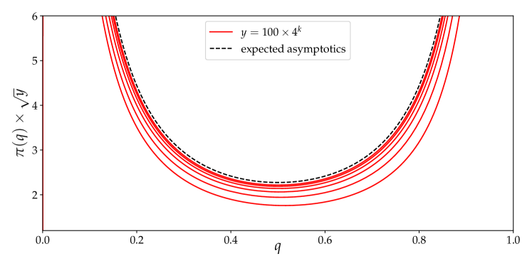
Figure 1: Distribution of the overlaps for different values of $y$ (set of full lines; $y=100\times 4^{k}$ with $k=1,\cdots,6$ increasing from bottom to top) and $X-X_{y}$ set to $\sqrt{2}\,y^{1/4}$, together with the expected asymptotics given in Eq. (69) (dashed line).

The equation to solve to get the equivalent of $G$ in the framework of this model is the following:

$$G(y+\delta y,x;y_{1})=\frac{1}{2}(1-\delta y)\left[G(y,x-\delta x;y_{1})+G(y,x+\delta x;y_{1})\right]+2\delta y\,G(y,x;y_{1})\,S(y,x),$$ (73)

with

$$G(y_{1},x;y_{1})=\left[1-S(y_{1},x)\right]^{2}.$$ (74)

(Compare to Eq. (10) and (11) respectively obtained in the dipole model).

In order to satisfy in some optimal way the double constraint in Eq. (24), we set $x$ to a value $X$ such that

$$X\simeq X_{y}+\sqrt{\kappa}\,y^{1/4},$$ (75)

where $\kappa$ is a constant that we shall pick in the set $\{1,2,4\}$. In general, we cannot achieve the equality because $X$ is the position of a lattice site, so it is discrete, while the r.h.s. is a real number: We have picked the closest site to the left of the position in the r.h.s. Up to a numerical factor, the r.h.s. is the geometric average of the two bounds on $X-X_{y}$ in Eq. (24). Varying this constant enables one to go more or less deep in the scaling region.

We have collected data for $y$ up to ${\cal O}(10^{6})$. We plot the distribution $\pi_{y}(q)$ at finite rapidity rescaled by $\sqrt{y}$ for different $y$ and $\kappa$ in Fig. 1, together with the expected infinite-$y$ asymptotic distribution $\pi_{\infty}(q)$.

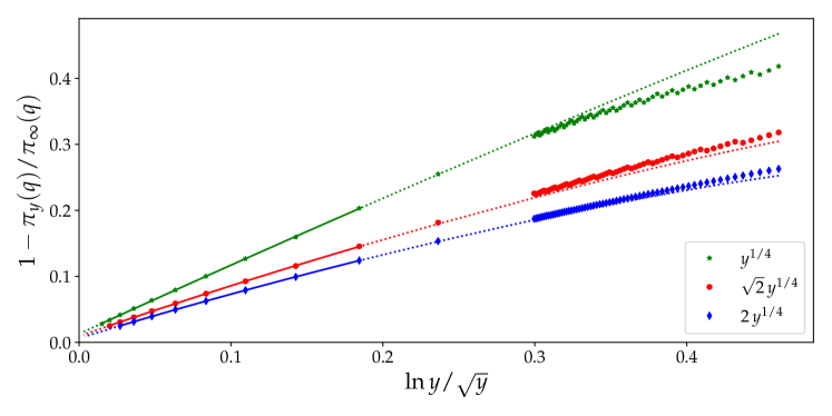
Figure 2: Complementary to 1 of the ratio between the probability of an overlap $q=0.5$ for different values of the total rapidity $y$ as a function of $\ln y/\sqrt{y}$. The points stem from the numerical integration of the evolution equations (70),(73),(74). The continuous lines, meant to guide the eye, represent the function (76) fitted to these points, and the dotted lines are extrapolations outside the domain in which the fit is performed.

In order to appreciate the convergence quantitatively, we pick a point of fixed $q$, and we compare the measured $\pi_{y}(q)$ at finite rapidity to the expected one $\pi_{\infty}(q)$ at $y=\infty$. In practice, we have chosen $q=0.5$, but we have also tried other values and got similar results for this ratio. We plot the complementary to one of this ratio against $\ln y/\sqrt{y}$ in Fig. 2. We expect a curve that goes through the origin: We see a quite good convergence of $1-\pi_{y}(q)/\pi_{\infty}(q)$ to 0 when $y\rightarrow\infty$.

Note that some non-smooth structures appear. They just reflect the discreteness of the model, which forces us to set $X$ to discrete values according to the procedure described above. The discretization step in $x$ is $\delta x=0.1$ in this model, which is not that small compared to $y^{1/4}$, even for very large $y$. So moving $X$ by $\delta x$ can lead to sizable differences in $\pi_{y}(q)$. Of course, these differences should get smaller and smaller as $y\rightarrow\infty$.

In order to guide the eye, we superimpose the following function to the data:

$$1-\frac{\pi_{y}(q=0.5)}{\pi_{\infty}(q=0.5)}\underset{\text{fit}}{=}a+\frac{b_{11}\ln y+b_{12}}{\sqrt{y}}.$$ (76)

We fit the parameters $a$, $b_{11}$, $b_{12}$, to the numerical calculations. We get reasonable values for all these parameters for the considered choices of $X$: $b_{11}$ and $b_{12}$ are of order 1, while $a$ is found close to zero; see Tab. 1. The constant $a$ is of the order of a percent, when we expect it to vanish. But we can hardly aim for better, because of the structures induced by the discreteness of the model, which makes the fitting procedure by a smooth function dependent on the choice of the points. Therefore, we conclude that our analytical formula (69) is well-supported by this numerical calculation.

However, these results show that the finite-$y$ corrections are definitely very large, and the convergence slow: Although we have computed $\pi_{y}$ for values of $y$ on the order of $10^{6}$, we have not managed to approach the asymptotics by better than about $3\%$. Figure 2 and the fitted formula (76) seem to indicate that the correction to $\pi_{\infty}(q)$ may take the form of a multiplicative factor $\left(1+\text{const}\times\ln y/\sqrt{y}\right)$. But we have no theory that may enable us neither to understand nor to guess the form of $\pi_{y}(q)$ beyond the leading term in the limit of large $y$.

We have also implemented independently another branching random walk model, and we have reached the same conclusion; see Appendix B for a presentation of the model and of the obtained results.

$X-X_{y}$	$a$ ($\times 10^{-2}$)	$b_{11}$	$b_{12}$
$y^{1/4}$	1.26	1.10	-0.519
$\sqrt{2}\,y^{1/4}$	0.909	0.896	-1.17
${2}\,y^{1/4}$	0.587	0.813	-1.28

Table 1: Values of the parameters in Eq. (76) obtained from a fit to the numerical data shown in Fig. 2.

5 Summary and outlook

In onium-nucleus scattering, in a frame in which the onium moves with a large rapidity $\tilde{y}_{0}$, the latter interacts through a typically dense quantum state made of gluons, that we represented by a set of color dipoles. Only a subset of these dipoles actually exchange energy with the nucleus. Having at least one dipole in this set is necessary to have a scattering event: This requirement defines the forward elastic scattering amplitude $T_{1}$. Calculating the joint probability $T_{2}$ to have a scattering and at least two dipoles in the set makes possible to get quantitative information on the correlations of the dipoles involved in the interaction.

In this paper, we have shown that the shape of the partonic configurations of an onium that interacts with a large nucleus depends qualitatively on the chosen reference frame. If the nucleus is highly boosted, namely if its rapidity $y_{0}$ is much larger than $\ln^{2}[r^{2}Q_{s}^{2}(y)]$, then the dipole distribution at the time of the interaction with the nucleus looks like a typical (“mean-field”) distribution just shifted (through a “front fluctuation” occurring in the very beginning of the evolution) towards larger sizes. If instead the nucleus is less boosted, $1\ll y_{0}\ll\ln^{2}[r^{2}Q_{s}^{2}(y)]$, then the dipoles which interact with it stem from a tip fluctuation occurring at much larger rapidities $\tilde{y}_{1}$ in the onium evolution, of order $y$ such that $y_{1}\sim y_{0}$.

Choosing a frame such that the tip fluctuation, the offspring of which scatter with the nucleus, be sufficiently developed, we were able to calculate the asymptotics of the distribution of the splitting rapidity of the slowest ancestor of the set of dipoles that effectively interact with the nucleus, including the overall constant. We have found that its ratio to the total rapidity of the scattering, a quantity that we denote by $q$, is distributed as

$${\pi}_{\infty}(q)=\frac{1}{\sqrt{y}}\frac{1}{\gamma_{0}\sqrt{2\pi\chi^{\prime\prime}(\gamma_{0})}}\frac{1}{q^{3/2}(1-q)^{3/2}}.$$ (77)

This expression holds when the size $r$ of the onium is chosen in the so-called scaling region, defined as

$$1\ll\ln^{2}\frac{1}{r^{2}Q_{s}^{2}(y)}\ll y,\quad\text{namely}\quad 1\ll(x-X_{y})^{2}\ll y,$$ (78)

where $x$ and $X_{y}$ just correspond to $1/r$ and $Q_{s}(y)$ respectively when measured on a logarithmic scale (see Eq. (14)), and $X_{y}=\chi^{\prime}(\gamma_{0})y-\frac{3}{2\gamma_{0}}\ln y$. Equation (77) is our main quantitative result. A particular realization of the model introduced in Sec. 4 and used to check numerically the calculations is shown in Fig. 3.

After identification of the rapidity with a time variable, we expect this expression to represent the distribution of the relative branching time of the most recent common ancestor of all particles that end up to the right of some predefined position $x$ for any branching random walk – provided that $x$ is chosen in the scaling region. (This $q$ is also called “overlap” in the statistical physics literature). The constants that appear in these expressions are easily calculated from the detailed form of the elementary processes which define the branching random walk.

We observe that our result coincides with a conjecture by Derrida and Mottishaw [34] for a slightly different genealogy problem in the context of general branching random walks: They computed the distribution of the branching time of the most recent common ancestor of two particles of predefined order number counted from the tip of the particle distribution at some given large time. To make contact between our equation (77) and the formula (6) they wrote down in Ref. [34], we just need to identify our $\pi(q)$ with their $p(q)$, $y$ with the total evolution time $t$, $\gamma_{0}$ with $\beta_{c}$, and $\chi^{\prime\prime}(\gamma_{0})$ with $\beta_{c}\,v^{\prime\prime}(\beta_{c})$. The constant $\chi^{\prime}(\gamma_{0})$, that enters the validity condition, is just to be identified with the critical FKPP front velocity $v(\beta_{c})$.

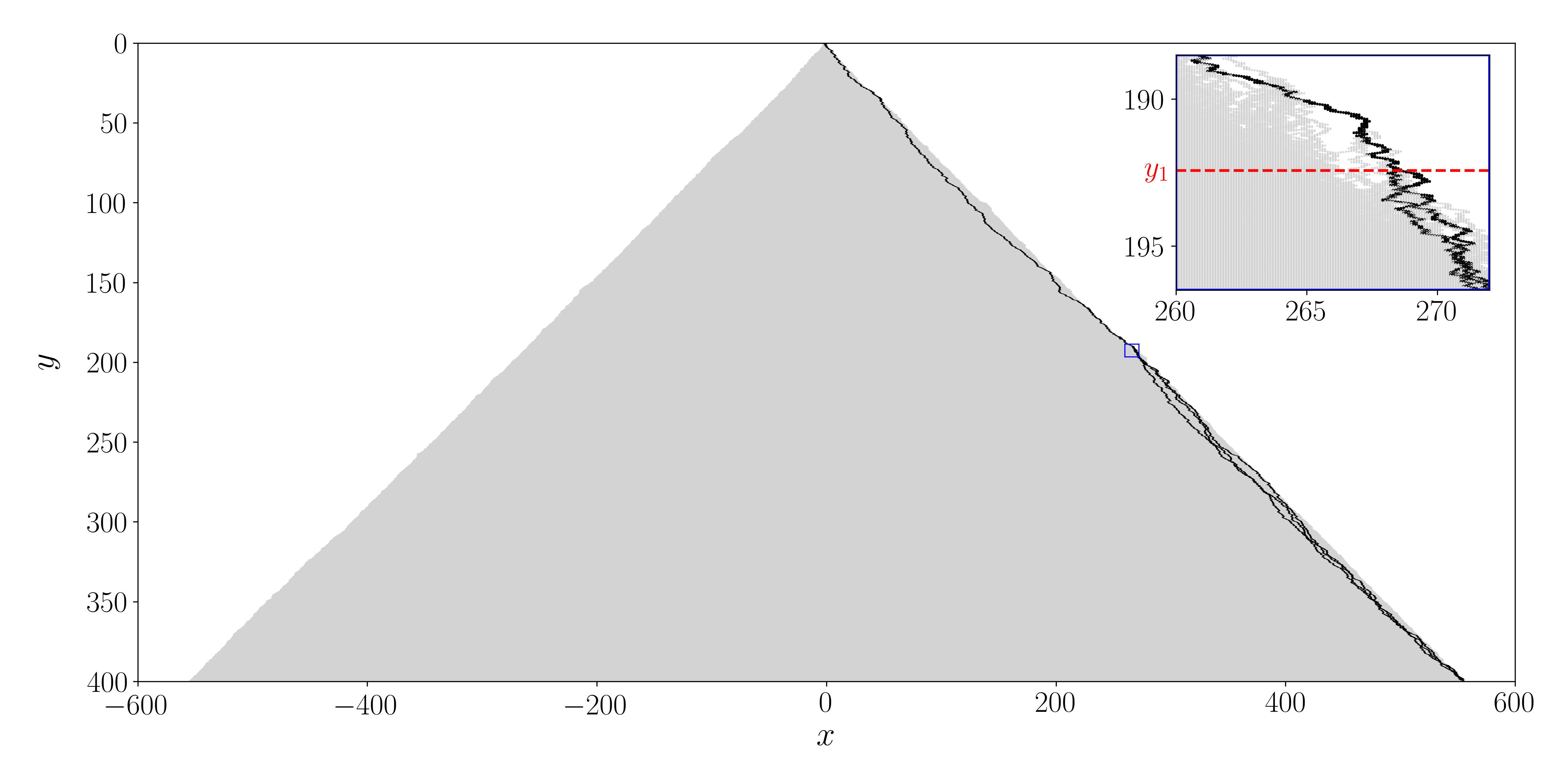
Figure 3: One particular realization of the toy model described in Sec. 4 evolved up to $y=400$, that turns out to possess several particles to the right of the position $X\simeq X_{y=400}+\sqrt{2}\times{400}^{1/4}$. The grey zone is the set of non-empty lattice sites for all values of the rapidity. The black lines represent the worldlines of all the particles that end up with a position not less than $X$ at the final rapidity $y=400$. The common ancestor of these particles splits at $y_{1}=192.43$. The inset is a zoom on the branching region around the branching rapidity $y_{1}$, illustrating that this common ancestor indeed stems from a large fluctuation occurring at a rapidity close to $y_{1}$, as assumed in the phenomenological model. This rare realization was generated using the algorithm proposed in Ref. [33].

While this expression was established in [34] through a calculation in the framework of the Generalized Random Energy Model [35], we have derived it in the context of the problem we were addressing from the phenomenological model for branching random walks, which just assumes that the time evolution is essentially deterministic, except for one single fluctuation. Proving our result for the genealogies rigorously, establishing a framework for the systematic calculation of corrections, crucial for applications since the approach to the asymptotics turns out to be very slow, are problems of general interest for branching processes, and exciting challenges for further investigations.

Also, our method would not apply to the specific genealogy problems Derrida-Mottishaw were addressing: While the $y$ (or $t$)-dependence would turn out correct, the overall constant could not be obtained. The reason for this is that we do not have a sufficient understanding of the particle distributions and of their correlations very close to the lead particle. Trying to build a good picture of the latter [36, 32, 33] is a long-term program that deserves more efforts.

As for the more specialized diffraction problem, which was the initial motivation for the present work, we also intend to try and extend our calculation to the rate of rapidity gaps in high-energy onium-nucleus scattering. The main crucial difference is that the latter being a quantum mechanical observable, it has no interpretation in purely classical probabilistic terms. However, preliminary investigations seem to indicate that the technical tools developed here can be applied also to that observable, which will be measurable at a future electron-ion collider. Of course, the finite-rapidity $y$ subasymptotics (presumably of relative order $\ln y/\sqrt{y}$) will also be significant for these observables in the kinematics of actual experiments. The systematic calculation of such corrections is presently not within reach, but it would be an exciting and useful interdisciplinary program.

Appendix A A few useful integrals

The calculations presented in the body of this paper require to perform a few integrals. Let us introduce the following notations:

$$I_{k}(A)\equiv\int_{1}^{\infty}\frac{dt}{t^{2}}\left[1-\sum_{i=0}^{k-1}\frac{(At)^{i}}{i!}e^{-At}\right]\quad\text{and}\quad I^{\prime}_{k}(A)\equiv\int_{1}^{\infty}\frac{dt}{t^{2}}\ln t\,\left[1-\sum_{i=0}^{k-1}\frac{(At)^{i}}{i!}e^{-At}\right].$$ (79)

We will study the following particular cases:

$$I_{1}(A) \equiv\int_{1}^{\infty}\frac{dt}{t^{2}}\left(1-e^{-At}\right) I_{1}^{\prime}(A) \equiv\int_{1}^{\infty}\frac{dt}{t^{2}}\ln t\left(1-e^{-At}\right)$$ (80)

$$I_{2}(A) \equiv\int_{1}^{\infty}\frac{dt}{t^{2}}\left[1-(1+At)e^{-At}\right] I_{2}^{\prime}(A) \equiv\int_{1}^{\infty}\frac{dt}{t^{2}}\ln t\,\left[1-(1+At)e^{-At}\right]$$ (81)

Although these integrals have exact expressions in terms of special functions, only the small-$A$ limits will be relevant for our purpose.

These integrals can be deduced from more general ones:

$$\begin{split}I_{1,\varepsilon}(A)&\equiv\int_{1}^{\infty}\frac{dt}{t^{2-\varepsilon}}\left(1-e^{-At}\right)=\frac{1}{1-\varepsilon}\left[1-e^{-A}+\Gamma(\varepsilon,A)A^{1-\varepsilon}\right],\\ I_{2,\varepsilon}(A)&\equiv\int_{1}^{\infty}\frac{dt}{t^{2-\varepsilon}}\left[1-(1+At)e^{-At}\right]=\frac{1}{1-\varepsilon}\left[1-e^{-A}+\varepsilon\Gamma(\varepsilon,A)A^{1-\varepsilon}\right],\end{split}$$ (82)

where $\Gamma$ is the incomplete Gamma function:

$$\Gamma(\varepsilon,A)\equiv\int_{A}^{\infty}d\bar{t}\,{\bar{t}}^{\varepsilon-1}e^{-\bar{t}}.$$ (83)

We want to calculate the leading term in the small-$A$ limit of the expansion of these integrals to order $\varepsilon$. To this aim, we write

$$\begin{split}\Gamma(\varepsilon,A)&=\frac{1}{\varepsilon}\left[\Gamma(1+\varepsilon)-A^{\varepsilon}+{\cal O}(A)\right]\\ &=\ln\frac{1}{A}-\gamma_{E}+{\cal O}(A)+\frac{\varepsilon}{2}\left[\psi^{\prime}(1)-\ln^{2}\frac{1}{A}+{\cal O}(A)\right]+\cdots\end{split}$$ (84)

Thus

$$I_{1}(A)=A\,\ln\frac{1}{A}+{\cal O}(A)\quad\text{and}\quad I_{1}^{\prime}(A)=\frac{A}{2}\ln\frac{1}{A}\left[\ln\frac{1}{A}+2(\psi(1)+1)\right]+{\cal O}(A).$$ (85)

Note that the factor $A$ is dimensional, while $1/A$ in the argument of the logarithm is just the size of the relevant integration region, which extends to $\sim 1/A$. Actually, the integral could also be performed by simply restricting the integration region to $[1,\kappa/A]$, where $\kappa\sim{\cal O}(1)$, and expanding the exponential: The overall normalization of the leading term for $A\ll 1$ would be identical to the one found from the exact calculation. The details of how the integration region is effectively cut off in the integrand do not matter.

As for $I_{2}$ and $I_{2}^{\prime}$, we expand $I_{2,\varepsilon}$ to order $\varepsilon$. We arrive at the following exact expressions, together with their expansion at lowest order for $A\ll 1$:

$$I_{2}(A)=1-e^{-A}\simeq A[1+{\cal O}(A)]\quad\text{and}\quad I_{2}^{\prime}(A)=A\,\Gamma(0,A)\simeq A\,\ln\frac{1}{A}+{\cal O}(A).$$ (86)

Note that $I_{1}$ and $I_{2}^{\prime}$ are identical for small $A$. However, $I_{2}^{\prime}$ is not a logarithmic integral, and therefore, the overall constant factor of the leading term in the limit $A\ll 1$ of interest here is sensitive to the detailed form of the integrand.

Appendix B Numerical calculations in an alternative model

The branching random walk model defined and studied in Sec. 4 was actually a particular discretization, in space and time, of a branching Brownian motion. The FKPP equation [10, 11], that is solved e.g. by the probability that there is at least a particle to the right of some predefined $X$, when the diffusion constant of the Brownian process is set to $D$, reads

$$\partial_{y}T_{1}=D\,\partial_{x}^{2}T_{1}+T_{1}(1-T_{1}).$$ (87)

Equation (70) for $S=1-T_{1}$ is a particular lattice discretization of (87), with $D=\frac{1}{2}$.

In this Appendix, we shall study an alternative discretization, namely

$$T_{1}(y+\delta y,x)-T_{1}(y,x)=\frac{\delta y}{\delta x^{2}}\left[T_{1}(y,x+\delta x)-2T_{1}(y,x)+T_{1}(y,x-\delta x)\right]+\delta y\,T_{1}(y,x)[1-T_{1}(y,x)].$$ (88)

We would recover Eq. (87) with $D=1$ in the joint limit $\delta y,\delta x\rightarrow 0$.

The underlying branching random walks are actually quite different in the two discretization schemes. In the present scheme, a particle on a given site has a probability to move, either left or right, of order $\delta y$, which is taken small. In the previous scheme instead, it had a probability $1-\delta y$ to move.

In this new scheme, the evolution equation for $G$ reads, for $y>y_{1}$,

$$G(y+\delta y,x;y_{1})-G(y,x;y_{1})=\frac{\delta y}{\delta x^{2}}\left[G(y,x+\delta x;y_{1})-2G(y,x;y_{1})+G(y,x-\delta x,y;y_{1})\right]\\ +\delta y\,G(y,x;y_{1})[1-2T_{1}(y,x)],$$ (89)

and the initial condition is the same as in the previous model, see Eq. (74).

We have set $\delta y=0.02$ and $\delta x=0.25$, which leads to the following value of the constants entering the asymptotic quantities of interest:

$$\gamma_{0}=1.0120279\cdots,\quad\chi^{\prime}(\gamma_{0})=1.9659159\cdots,\quad\chi^{\prime\prime}(\gamma_{0})=1.9065278\cdots$$ (90)

These parameters are quite different from those of the first model; Compare to Eq. (72). We have also chosen a different initial condition: $T_{1}(y=0,x)=1-\exp(e^{-4\gamma_{0}x})$.

Our implementation of these evolution equations is independent of the one of the first model, and the very numerical methods used are different. As for the model exposed here, we evolve $\ln T_{1}$ and $\ln G$ instead of $T_{1}$ and $G$ directly, at variance with the first model, in order to make sure that we treat accurately-enough the crucial region in which these functions take very small values (see e.g. [30] for a description of such a numerical method).

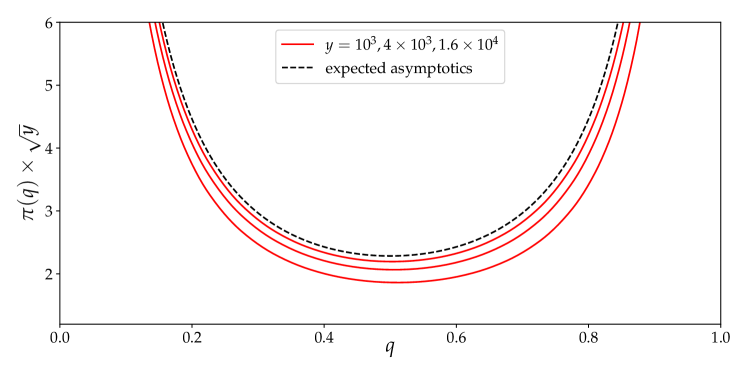
Figure 4: Distribution of the overlaps for different values of $y$ (set of full lines; $y\in\{10^{3},4\times 10^{3},1.6\times 10^{4}\}$ increasing from bottom to top) and $X-X_{y}$ set to $\sqrt{2}\,y^{1/4}$, together with the expected asymptotics given in Eq. (69) with the constants (90) (dashed line).

The overlaps $\pi_{y}(q)$, shown in Fig. 4 for $y\in\{10^{3},4\times 10^{3},1.6\times 10^{4}\}$, are compatible with a convergence to the expected asymptotics (69) – although it is more difficult to judge than for the first numerical model: The maximum value of $y$ for which we have been able to perform the calculation is more than one order of magnitude smaller than in the case of the latter.

References

- [1] N. N. Nikolaev and B. Zakharov, Z. Phys. C 49, 607 (1991).
- [2] C. Ewerz and O. Nachtmann, Annals Phys. 322, 1670 (2007), hep-ph/0604087.
- [3] A. Accardi et al., Eur. Phys. J. A 52, 268 (2016), arXiv:1212.1701 [nucl-ex].
- [4] P. Agostini et al. [LHeC and FCC-he Study Group], “The Large Hadron-Electron Collider at the HL-LHC,” arXiv:2007.14491 [hep-ex].
- [5] Y. V. Kovchegov and K. Tuchin, Phys. Rev. D 65, 074026 (2002), hep-ph/0111362.
- [6] A. H. Mueller and S. Munier, Nucl. Phys. A893, 43 (2012), 1206.1333.
- [7] Y. V. Kovchegov and E. Levin, Quantum chromodynamics at high energy, Vol. 33 (Cambridge University Press, 2012).
- [8] I. Balitsky, Nucl. Phys. B463, 99 (1996), hep-ph/9509348.
- [9] Y. V. Kovchegov, Phys. Rev. D61, 074018 (2000), hep-ph/9905214.
- [10] R. A. Fisher, Annals of Eugenics 7, 355 (1937).
- [11] A. Kolmogorov, I. Petrovsky, and N. Piscounov, Bull. Univ. État Moscou A 1, 1–25 (1937).
- [12] W. van Saarloos, Physics Reports 386, 29 (2003).
- [13] É. Brunet, Some aspects of the Fisher-KPP equation and the branching Brownian motion, Habilitation à diriger des recherches, UPMC, 2016, https://tel.archives-ouvertes.fr/tel-01417420/file/hdr.pdf.
- [14] S. Munier, Phys. Rept. 473, 1 (2009), arXiv:0901.2823 [hep-ph].
- [15] S. Munier and R. B. Peschanski, Phys. Rev. Lett. 91, 232001 (2003), hep-ph/0309177.
- [16] A. H. Mueller, Nucl. Phys. B415, 373 (1994).
- [17] Y. V. Kovchegov and E. Levin, Nucl. Phys. B577, 221 (2000), hep-ph/9911523.
- [18] A. M. Stasto, K. J. Golec-Biernat, and J. Kwiecinski, Phys. Rev. Lett. 86, 596 (2001), hep-ph/0007192.
- [19] J.-P. Blaizot, E. Iancu, and D. Triantafyllopoulos, Nucl. Phys. A 784, 227 (2007), hep-ph/0606253.
- [20] A. H. Mueller and S. Munier, Phys. Rev. Lett. 121, 082001 (2018), arXiv:1805.09417 [hep-ph].
- [21] A. H. Mueller and S. Munier, Phys. Rev. D98, 034021 (2018), 1805.02847.
- [22] L. D. McLerran and R. Venugopalan, Phys. Rev. D49, 2233 (1994), hep-ph/9309289.
- [23] A. H. Mueller and D. N. Triantafyllopoulos, Nucl. Phys. B640, 331 (2002), hep-ph/0205167.
- [24] R. Enberg, K. J. Golec-Biernat, and S. Munier, Phys. Rev. D 72, 074021 (2005), hep-ph/0505101.
- [25] J. Albacete, N. Armesto, J. Milhano, C. Salgado, and U. Wiedemann, Phys. Rev. D 71, 014003 (2005), hep-ph/0408216.
- [26] D. Le Anh, Internship report, École polytechnique (unpublished), 2018.
- [27] D. Le Anh, Diffractive dissociation in onium–nucleus scattering from a partonic picture, Presented at EDS Blois 2019 Conference, Quy Nhon, Vietnam in 18th Conference on Elastic and Diffractive Scattering, 2019, arXiv:1910.03953 [hep-ph].
- [28] S. K. Grossberndt, “Second order twist contributions to the Balitsky-Kovchegov equation at small-: Deterministic and stochastic pictures”, 2020, arXiv:2003.09303 [hep-ph].
- [29] L. Motyka, M. Sadzikowski, and W. Slominski, Phys. Rev. D 86, 111501 (2012), 1203.5461.
- [30] A. H. Mueller and S. Munier, Phys. Rev. E90, 042143 (2014), 1404.5500.
- [31] A. H. Mueller and S. Munier, Phys. Lett. B737, 303 (2014), 1405.3131.
- [32] A. D. Le, A. H. Mueller, and S. Munier, “Monte Carlo study of the tip region of branching random walks evolved to large times”, 2020, arXiv:2003.04362 [cond-mat].
- [33] É. Brunet, A. D. Le, A. H. Mueller, and S. Munier, EPL (Europhysics Letters) 131, 40002 (2020).
- [34] B. Derrida and P. Mottishaw, EPL (Europhysics Letters) 115, 40005 (2016).
- [35] Derrida, B., J. Physique Lett. 46, 401 (1985).
- [36] É. Brunet and B. Derrida, Journal of Statistical Physics 143, 420 (2011).