Relativistic rank-one separable kernel for helium-3 charge form factor

Abstract

Elastic electron-helium-3 scattering is studied in the relativistic impulse approximation. The amplitudes for the three-nucleon system are obtained by solving the relativistic generalization of the Faddeev equations with a separable rank-one kernel of the nucleon-nucleon interaction. The contribution of partial-wave states with nonzero orbital moment of a nucleon pair is investigated. The static approximation and additional relativistic corrections for the ${}^{3}{\rm He}$ charge form factor are calculated for the momentum transfer squared up to 100 fm^-2. The contribution of the ${}^{3}D_{1}$ partial-wave state and relativistic corrections are found to be sizable at high energies.

1 Introduction

The study of electron-nucleus reactions is important for obtaining information on the nucleon-nucleon (NN) interaction, which is crucial for understanding the structure of strong interactions. At present, a lot of experimental data are known for the reaction cross sections and polarization observables. Of great interest is the intermediate range of energies in these reactions where the nonrelativistic description based on the potential or nonrelativistic meson-nucleon models does not properly work. On the other hand, Quantum Chromodynamics, which operates with quark and gluon degrees of freedom, also does not give an appropriate description in this region.

The latest experimental data for elastic electron-deuteron/helium scattering (for example [1, 2], for ${}^{3}{\rm He}$ elastic form factors at high momentum transfer squared up to 60-100 fm^-2), require taking into account the relativistic treatment of nuclear systems.

One of the promising relativistic approaches is the covariant formalism based on the Bethe-Salpeter equation for two nucleons [3]. This approach operates with relativistic meson-nucleon degrees of freedom. There are a lot of investigations of two-nucleon systems and their reactions ([4, 5, 6, 7, 8], see also the comprehensive review [9]).

Calculations with covariant separable kernels of NN interaction are also widely used. The results of the investigations for the elastic electron-deuteron scattering can be found in [10, 11, 12, 13, 14, 15].

Using the NN interaction to calculate three-nucleon (3N) systems may shed light on the occurrence of non-nucleonic degrees of freedom or effective 3N forces. The Faddeev equations [16] are usually used (see also [17]) to study three-particle systems in quantum mechanics. The equations describe these systems with pair potentials of any kind as bound and scattering states. The relativistic generalization of the Faddeev equations can be applied to a system of three relativistic particles [18, 19, 20, 21, 22]. In this case, the relativistic two-particle T matrix is taken as a solution of the Bethe-Salpeter equation (we call such a three-particle equation the Bethe-Salpeter-Faddeev equation, BSF).

Among the relativistic methods for the three-nucleon system, one should also note the relativistic approach, which uses the covariant spectator theory (CST) to construct the three-nucleon wave function [23, 24] and the variational Monte Carlo calculations with the relativistic Hamiltonian [25].

One of the important physical problems is to give the right location of the first diffraction minimum of the three-nucleon charge form factor. In the review [9], three different relativistic theoretical approaches are considered for the form factors of the two- and three-nucleon systems: one is based on realistic interactions and currents, including relativistic corrections, the other relies on a chiral effective field theory description of strong interactions in nuclei and the last one is CST. For momentum transfers squared below 25 fm^-2 there is satisfactory agreement between experimental data and theoretical results in all three approaches. However, above 25 fm^-2 a relativistic treatment of the dynamics is necessary.

To solve the BSF equation, it is necessary to know the potential of the nucleon-nucleon interaction in the explicit form. The separable kernels of NN interactions can be used [18, 19, 20, 21, 22] to simplify the calculations. In recent works, we have solved the BSF equation for rank-one separable kernels of NN interactions and took into account the two-nucleon states with the total angular momentum $j=0-1$ [26]. For the sake of simplicity, we considered the nucleon propagators in the scalar-particle form while the spin-isospin dependence was treated by applying the recoupling matrix [22]. The form factors of the potential were the relativistic Yamaguchi functions [27, 28].

One of the problems of the numerical solution of the BSF equations is that the solution is usually obtained in Euclidean space, while the calculation of the electromagnetic (EM) reaction observables requires a relativistic wave function in Minkowski space. It should be noted that there are papers on such a difficult task [29, 30]. Another way is to carry out the Taylor series expansion of the corresponding arguments.

Relativistic calculations for elastic electron scattering off ³He were considered in several papers [31, 32, 33, 18, 19]. In [34], we studied the sensitivity of unpolarized elastic electron scattering off ³He to nucleon EM form factors in the static approximation.

In the present paper, we considered two types of additional effects: the contribution of partial-wave states with nonzero orbital moment of a nucleon pair and the relativistic corrections for the ${}^{3}{\rm He}$ charge form factor. The latter are due to the full Lorentz transformation of the four-momentum of the one-nucleon propagator, the residue at a simple pole on the complex variable $q_{0}$ and the terms of a Taylor series expansion of the arguments of the outgoing particle wave function.

The paper is organized as follows: in Sec. 2, the expressions for the charge ³He form factor are given, in Sec. 3 the static approximation and relativistic corrections are defined, in Sec. 4 the calculations and results are discussed and finally the conclusion is given.

2 Form factors of a three-nucleon system

As a system with one-half spin, the electromagnetic current of ³He can be parameterized by two elastic form factors: charge (electric) $F_{\rm C}$ and magnetic $F_{\rm M}$ (see for example, [17]). In calculations, we use a straightforward relativistic generalization of the nonrelativistic expression for the ³He charge form factor, which has the following form [37, 38, 17, 18]:

$$2F_{\rm C}=(2F^{p}_{\rm C}+F^{n}_{\rm C})F_{1}-\frac{2}{3}(F^{p}_{\rm C}-F^{n}_{\rm C})F_{2}+2(F^{n}_{\rm C}-F^{p}_{\rm C})F_{3},$$ (1)

where $F^{p,n}_{\rm C}$ is the charge form factor of the proton and neutron, respectively.

The functions $F_{1,2,3}$ can be expressed in terms of the wave functions of the three-nucleon system. In the relativistic impulse approximation, they can be written as follows:

$$F_{1}({\hat{Q}})=\int d^{4}{{\hat{p}}}\int d^{4}{{\hat{q}}}\,G_{1}^{\prime}({\hat{k}}^{\prime}_{1})\,G_{1}({\hat{k}}_{1})\,G_{2}({\hat{k}}_{2})\,G_{3}({\hat{k}}_{3})\,\sum_{i=1}^{3}\Psi^{*}_{i}({\hat{p}},{\hat{q}};{\hat{P}})\,\Psi_{i}({\hat{p}},{\hat{q}}^{\prime};{\hat{P}}^{\prime}),$$

$$F_{2}({\hat{Q}})=-3\int d^{4}{{\hat{p}}}\int d^{4}{{\hat{q}}}\,G_{1}^{\prime}({\hat{k}}^{\prime}_{1})\,G_{1}({\hat{k}}_{1})\,G_{2}({\hat{k}}_{2})\,G_{3}({\hat{k}}_{3})\,\Psi^{*}_{1}({\hat{p}},{\hat{q}};{\hat{P}})\,\Psi_{2}({\hat{p}},{\hat{q}}^{\prime};{\hat{P}}^{\prime}),$$

$$F_{3}({\hat{Q}})=\int d^{4}{{\hat{p}}}\int d^{4}{{\hat{q}}}\,G_{1}^{\prime}({\hat{k}}^{\prime}_{1})\,G_{1}({\hat{k}}_{1})\,G_{2}({\hat{k}}_{2})\,G_{3}({\hat{k}}_{3})\,\Psi^{*}_{3}({\hat{p}},{\hat{q}};{\hat{P}})\,\Psi_{4}({\hat{p}},{\hat{q}}^{\prime};{\hat{P}}^{\prime}),$$ (2)

where ${\hat{Q}}$ is the four-momentum transfer, ${\hat{p}}$ and ${\hat{q}},{\hat{q}}^{\prime}={\hat{q}}-\frac{2}{3}{\hat{Q}}$ are the Jacobi four-momenta of the three-nucleon system, and ${\hat{P}},{\hat{P}}^{\prime}={\hat{P}}+{\hat{Q}}$ are the total four-momenta. The nucleon propagators read:

$$G_{1}({\hat{k}}_{1})=\left[(\frac{1}{3}{\hat{P}}-{\hat{q}})^{2}-m_{N}^{2}+i\epsilon\right]^{-1},$$ (3)

$$G_{1}^{\prime}({\hat{k}}_{1}^{\prime})=\left[(\frac{1}{3}{\hat{P}}^{\prime}-{\hat{q}}^{\prime})^{2}-m_{N}^{2}+i\epsilon\right]^{-1},$$

$$G_{2}({\hat{k}}_{2})=\left[(\frac{1}{3}{\hat{P}}+\frac{1}{2}{\hat{q}}+{\hat{p}})^{2}-m_{N}^{2}+i\epsilon\right]^{-1},$$

$$G_{3}({\hat{k}}_{3})=\left[(\frac{1}{3}{\hat{P}}+\frac{1}{2}{\hat{q}}-{\hat{p}})^{2}-m_{N}^{2}+i\epsilon\right]^{-1},$$

where $m_{N}$ is the nucleon mass and the infinitesimal negative addition to nucleon mass defines how to treat propagator singularities.

The three-nucleon wave functions $\Psi_{i}$ can be expressed in terms of the following functions:

$$\Psi_{1}=A(1)+A(2)+A(3),$$ (4)

$$\Psi_{2}=\frac{1}{2}(B(2)+B(3)-2B(1))+\frac{\sqrt{3}}{2}(C(3)-C(2)),$$

$$\Psi_{3}=\frac{\sqrt{3}}{2}(B(3)-B(2))-\frac{1}{2}(C(3)+C(2)-2C(1)),$$

$$\Psi_{4}=D(1)+D(2)+D(3),$$

which are related to the spin-isospin $a(s,i)$ states of the two-particle subsystem:

$$A(n)=\frac{1}{\sqrt{2}}(u_{3}(n)-u_{1}(n)),$$ (5)

$$B(n)=\frac{1}{\sqrt{2}}(u_{3}(n)+u_{1}(n)),$$

$$C(n)=\frac{1}{\sqrt{2}}(u_{2}(n)-u_{4}(n)),$$

$$D(n)=-\frac{1}{\sqrt{2}}(u_{2}(n)+u_{4}(n))$$

where $n$ is the number of a particle.

The functions $u_{a}$ correspond to the following two-nucleon sub-states:

$$a=1:(s,i)=(1,0)[^{3}S_{1},^{3}D_{1}],$$ (6)

$$a=2:(s,i)=(1,1)[^{3}P_{0},^{3}P_{1}],$$

$$a=3:(s,i)=(0,1)[^{1}S_{0}],$$

$$a=4:(s,i)=(0,0)[^{1}P_{1}].$$

We consider various combinations of the spin, isospin and momenta of the three nucleons under their permutations, to satisfy the Pauli principle (the ³He vertex function must be antisymmetric with respect to permutation of any pair of particles) to obtain above-mentioned equations (see details in [37, 38]).

The wave functions $u_{a}$ can be related to the vertex functions, which are the BSF equation solutions $\Phi_{a}$. The relations in the center-of-mass (c.m.) frame of the three-nucleon system ${\hat{P}}_{c.m.}=(\sqrt{s},\mathbf{0})$ read:

$$u_{a}({\hat{p}},{\hat{q}})=\sum_{l\lambda LM_{L}}\,{\cal Y}_{l\lambda LM}(\mathbf{n_{p}},\mathbf{n_{q}})\,g_{l}^{a}(p_{0},p)\,\tau_{l}^{a}[(\frac{2}{3}\sqrt{s}+q_{0})^{2}-\mathbf{q}^{2}]\,\Phi^{a}_{l\lambda L}(q_{0},q),$$

$${\cal Y}_{l\lambda LM_{L}}(\mathbf{n_{p}},\mathbf{n_{q}})=\sum_{m\mu}(lm\lambda\mu|LM_{L}){Y}_{lm}(\mathbf{n_{p}}){Y}_{\lambda\mu}(\mathbf{n_{q}}).$$ (7)

The form of (7) is a consequence of using the kernel of NN interaction in a separable form. Here $(.|.)$ is the Clebsch-Gordan coefficient, ${Y}_{lm}(\mathbf{n})$ are spherical harmonics, $l$ and $m$ are the two-particle subsystem angular momentum and its projection, $\lambda$ and $\mu$ are the angular momentum of the third particle relative to the two-particle subsystem and its projection, $L$ and $M_{L}$ are the total angular momentum and its projection, $g_{l}^{a}$ are the form factors of the NN interaction kernel and $\tau_{l}^{a}$ is the relativistic two-particle propagator of interacting nucleons.

In the previous paper [34], the calculations were carried out using only the ${}^{1}S_{0},^{3}S_{1}$ partial-wave states. In this paper, the $D$ and $P$ partial-wave states are added and their contributions are considered.

To calculate the functions $F_{1,2,3}$ (2), it is convenient to use the Breit reference system that is defined as follows:

$${\hat{Q}}=(0,\mathbf{Q}),\qquad{\hat{P}}=(E_{B},-\frac{\mathbf{Q}}{2}),\qquad{\hat{P}}^{\prime}=(E_{B},\frac{\mathbf{Q}}{2}),$$ (8)

with $E_{B}=\sqrt{{\mathbf{Q}}^{2}/4+s}$. Also, $\sqrt{s}=M_{t}=3m_{N}-E_{t}$ and $E_{t}$ are the mass and the binding energy of a three-nucleon bound state, respectively.

The solutions of the BSF equations $\Psi_{i}$ in (2), however, have been found in the c.m. (rest) frames of the corresponding three-nucleon systems. To relate the Breit and initial particle c.m. frames, the Lorentz transformation ${\rm L}$ should be applied to the four-momenta:

$${\hat{P}}={\rm L}{\hat{P}}_{c.m.},\qquad{\hat{p}}={\rm L}{\hat{p}}_{c.m.},\qquad{\hat{q}}={\rm L}{\hat{q}}_{c.m.}.$$ (9)

The explicit form of the transformation ${\rm L}$ can be obtained by using (8). Let us assume the boost of the system to be along the $Z$ axis:

$${\rm L}=\left(\begin{array}[]{cccc}\sqrt{1+\eta}&0&0&-\sqrt{\eta}\\ 0&1&0&0\\ 0&0&1&0\\ -\sqrt{\eta}&0&0&\sqrt{1+\eta}\end{array}\right).$$ (14)

Here the parameter $\eta=\mathbf{Q}^{2}/4s$ is introduced. It is clear from (8) that the Breit and final particle c.m. frames are related as follows:

$${\hat{P}}^{\prime}={\rm L}^{-1}{\hat{P}}^{\prime}_{c.m.},\qquad{\hat{p}}^{\prime}={\rm L}^{-1}{\hat{p}}^{\prime}_{c.m.},\qquad{\hat{q}}^{\prime}={\rm L}^{-1}{\hat{q}}^{\prime}_{c.m.}.$$ (15)

Since the four-momenta ${\hat{q}}$ and ${\hat{q}}^{\prime}={\hat{q}}-\frac{2}{3}{\hat{Q}}$ are defined in different c.m. frames, the relations between their components are rather lengthy (we omit the c.m. labels):

$$q_{0}^{\prime}=(1+2\eta)\,q_{0}-2\sqrt{\eta}\sqrt{1+\eta}\,q_{z}+\frac{2}{3}\sqrt{\eta}\,Q,$$ (16)

$$q^{\prime}_{x}=q_{x}\qquad q^{\prime}_{y}=q_{y}$$

$$q^{\prime}_{z}=(1+2\eta)\,q_{z}-2\sqrt{\eta}\sqrt{1+\eta}\,q_{0}-\frac{2}{3}\sqrt{1+\eta}\,Q,$$

here $q_{z}=qy$ is the projection of momentum $\mathbf{q}$ onto the $Z$ axis and $y=\cos{\theta_{qQ}}$.

To summarize, the arguments of the initial and final particle wave functions and propagators were expressed in terms of the momenta calculated in the corresponding c.m. frames and related to each other using the Lorentz transformation. The Jacobian of the boost ${\rm L}$ is equal to one, so integration in (2) is performed on the $p$ and $q$ variables in the initial particle c.m. frame.

3 Static approximation and relativistic corrections

Using the results of the previous section, one can write for the propagators

$$G_{1}(q_{0},q)=\left[(\frac{1}{3}\sqrt{s}-q_{0})^{2}-\mathbf{q}^{2}-m_{N}^{2}+i\epsilon\right]^{-1},$$ (17)

$$G_{1}^{\prime}(q_{0}^{\prime},q^{\prime})=\left[(\frac{1}{3}\sqrt{s}-q^{\prime}_{0})^{2}-\mathbf{q}^{\prime 2}-m_{N}^{2}+i\epsilon\right]^{-1},$$

$$G_{2}(p_{0},p,q_{0},q)=\left[(\frac{1}{3}\sqrt{s}+(\frac{1}{2}q_{0}+p_{0}))^{2}-\mathbf{p}^{2}-\frac{1}{4}\mathbf{q}^{2}-{\mathbf{p}}\cdot{\mathbf{q}}-m_{N}^{2}+i\epsilon\right]^{-1},$$

$$G_{3}(p_{0},p,q_{0},q)=\left[(\frac{1}{3}\sqrt{s}+(\frac{1}{2}q_{0}-p_{0}))^{2}-\mathbf{p}^{2}-\frac{1}{4}\mathbf{q}^{2}+{\mathbf{p}}\cdot{\mathbf{q}}-m_{N}^{2}+i\epsilon\right]^{-1},$$

with ${\mathbf{p}}\cdot{\mathbf{q}}=pqx$ and $x=\cos{\theta_{pq}}$. The arguments of the final particle wave function are related to the initial ones by expressions (16).

Since the solutions of the BSF equations have been obtained in the Euclidean space [22] and are known only for real values of $q_{4}$, the simplest way to calculate (2) is to apply the Wick rotation procedure $p_{0}\to ip_{4},q_{0}\to iq_{4}$, if it is possible. Thus, one needs to investigate the analytic structure of the integrand on the complex-valued variables $p_{0},q_{0}$. The location of the variable $p_{0}$ singularities allows one to apply the Wick rotation procedure, although this is not true for the variable $q_{0}$ in general.

3.1 Static approximation

First, the so-called static approximation (SA) is considered. The SA assumes that all terms in the Lorentz transformation (16) proportional to $\eta$ are canceled:

$$q_{0}^{\prime}=q_{0},\qquad{\bf q^{\prime}}={\bf q}-\frac{2}{3}{\bf Q},$$ (18)

and these expressions are put as arguments into the propagator $G_{1}^{\prime}(k_{1}^{\prime})$ and final particle wave function $\Psi(p,q^{\prime})$:

$$G_{1}^{\prime}(q_{0}^{\prime},q^{\prime})\to\left[(\frac{1}{3}\sqrt{s}-q_{0})^{2}-\mathbf{q}^{2}-\frac{2}{3}{\mathbf{q}\cdot\mathbf{Q}}-\frac{4}{9}\mathbf{Q}^{2}-m_{N}^{2}+i\epsilon\right]^{-1},$$ (19)

$$\Psi_{i}(p_{0},p,q_{0}^{\prime},q^{\prime})\to\Psi_{i}(p_{0},p,q_{0},|{\bf q}-\frac{2}{3}{\bf Q}|),$$

with ${\mathbf{q}\cdot\mathbf{Q}}=qQy$.

Analyzing (19), one can see that the poles of $G_{1}^{\prime}$ on $q_{0}$ do not cross the imaginary $q_{0}$ axis and always stay in the second and fourth quadrants. In this case, the Wick rotation procedure $q_{0}\to iq_{4}$ can be applied.

The static approximation is similar to nonrelativistic calculations in that they use arguments (18) of the wave functions. However, the main difference is the dependence on $q_{0}$ of the wave functions and propagators that have positive and negative energy parts.

3.2 Relativistic corrections

Now we discuss the relativistic corrections (RC) to the SA. Second, the full expressions (16) for $q^{\prime}$ are used in $G_{1}^{\prime}(k_{1}^{\prime})$ and (18) in $\Psi(p,q^{\prime})$:

$$G_{1}^{\prime}=$$ (20)

$$\left[q_{0}^{2}+\frac{2}{3}\sqrt{s}(1+6\eta)q_{0}+4\sqrt{1+\eta}\sqrt{s}\sqrt{\eta}q_{z}-\frac{8}{3}\eta s+\frac{1}{9}s-{\mathbf{q}}^{2}-m_{N}^{2}+i\epsilon\right]^{-1},$$

$$\Psi_{i}(p_{0},p,q_{0}^{\prime},q^{\prime})\to\Psi_{i}(p_{0},p,q_{0},|{\bf q}-\frac{2}{3}{\bf Q}|).$$

Analyzing (20), one can see that for any $t=-{\hat{Q}}^{2}>-{\hat{Q}}_{min}^{2}=2/3\sqrt{s}(3m_{N}-\sqrt{s})$ the pole of $G_{1}^{\prime}$ on $q_{0}$ crosses the imaginary $q_{0}$ axis and appears in the third quadrant.

In this case, using the Cauchy theorem, one can transform the integrals over $p_{0}$, $q_{0}$ as follows:

$$\int_{-\infty}^{\infty}dp_{0}\int_{-\infty}^{\infty}dq_{0}\,\int_{0}^{\infty}dq\,\int_{-1}^{1}dy\,...\,f(p_{0},q_{0},p,q,x,y)=$$ (21)

$$-\int_{-\infty}^{\infty}dp_{4}\int_{-\infty}^{\infty}dq_{4}\,\int_{0}^{\infty}dq\,\int_{-1}^{1}dy\,...\,f(ip_{4},iq_{4},p,q,x,y)$$

$$+2\pi\mathop{\mathrm{Res}}_{q_{0}=q_{0}^{(2)}}\int_{-\infty}^{\infty}dp_{4}\,\int_{q_{min}}^{q_{max}}dq\,\int_{y_{min}}^{1}dy\,...\,f(ip_{4},q_{0},p,q,x,y),$$

where (…) means the two-fold integral $\int_{0}^{\infty}dp\,\int_{-1}^{1}dx$ and

$$q_{0}^{(1,2)}=\frac{\sqrt{s}}{3}(1+6\eta)\pm\sqrt{4\eta(1+\eta)s-4\sqrt{s}\sqrt{\eta}\sqrt{1+\eta}qy+\mathbf{q}^{2}+m_{N}^{2}}$$ (22)

are the simple poles of the propagator $G^{\prime}_{1}$.

The first integral on the right-hand side of (21) is a six-fold integral. The second one is a five-fold integral with the limits of integration on $q$ and $y$

$$q_{min,max}=2\sqrt{s}\sqrt{\eta}\sqrt{1+\eta}\mp\frac{1}{3}\sqrt{s+12\eta s+36\eta^{2}s-9m_{N}^{2}},$$ (23)

$$y_{min}=\frac{1}{36}\frac{24\eta s+9m_{N}^{2}+9\mathbf{q}^{2}-s}{q\sqrt{s}\sqrt{\eta}\sqrt{1+\eta}},\qquad\qquad y_{max}=1,$$ (24)

and the residue at the point $q_{0}=q_{0}^{(2)}$ is calculated. Remembering that the BSF solutions are known for real values of $q_{4}$ only, the following assumption was made:

$$\Psi(p_{0},p,q_{0}^{\prime},q^{\prime})\to g(p_{0},p)\,\tau[(\frac{2}{3}\sqrt{s}+q_{0}^{(2)})^{2}-{\bar{\mathbf{q}}}^{\prime 2}]\,\Phi(0,{\bar{q}}^{\prime}),$$

where value ${\bar{q}}^{\prime}$ is obtained using (16) with $q_{0}=q_{0}^{(2)}$.

Thus, two new effects appear: the Lorentz boost in the $G_{1}^{\prime}(k_{1}^{\prime})$ arguments, which gives a boost contribution (BC), and a simple pole on $q_{0}$, which gives an additional term in integrals – a pole contribution (PC).

Third, one can take into account the Lorentz boost of the arguments of the final ${}^{3}{\rm He}$ wave function. As was already mentioned, since the solutions of the BSF equations were obtained in the Euclidean space and are known only for real values of $q_{4}$, it is impossible to take into account the full Lorentz transformation of $q^{\prime}$. However, one can carry out a Taylor series expansion contribution (EC) around the point (18) on the parameter $\eta$.

The expansion of the function $\Phi(q^{\prime}_{4},q^{\prime})$ up to the first order of the parameter $\eta$ has the following form:

$$\Phi(iq^{\prime}_{4},q^{\prime})=\Phi(iq_{4},|\mathbf{q}-\frac{2}{3}\mathbf{Q}|)+\Big{[}C_{q_{4}}\frac{\partial}{\partial q_{4}}\Phi_{j}(iq_{4},q)\Big{]}_{q=|\mathbf{q}-\frac{2}{3}\mathbf{Q}|}$$

$$+\Big{[}C_{q}\frac{\partial}{\partial q}\Phi_{j}(iq_{4},q)\Big{]}_{q=|\mathbf{q}-\frac{2}{3}\mathbf{Q}|},$$ (25)

where

$$C_{q_{4}}=-i\left(2i\eta q_{4}-2\sqrt{\eta}\sqrt{1+\eta}qy+\frac{2}{3}\sqrt{\eta}Q\right),$$

$$C_{q}=\left(2\eta qy-2i\sqrt{\eta}\sqrt{1+\eta}q_{4}-\frac{2}{3}(\sqrt{1+\eta}-1)Q\right)y.$$

To exclude double counting, one needs to take into account only the second and third terms of the right-hand expression of (25) since the first term coincides with BC.

The derivative of the vertex function $\Phi$ can be found by differentiating the integral equation $\Phi=\int K\Phi$. In this case, the function $\Phi^{\prime}$ is determined by the integral $\Phi^{\prime}=\int K^{\prime}\Phi$ where $K^{\prime}$ is a derivative of the kernel of the integral equation.

4 Calculations and results

To calculate the functions $F_{1,2,3}$, the analytic expressions for $g^{a}(p)$ and $\tau^{a}(s,q)$ were used. The numerical solution for the functions $\Phi_{a}(q)$ was obtained by solving the system of homogeneous integral BSF equations by means of the Gaussian quadratures (see details in [20]) and then interpolated to the $(q_{4},q)$ points of integration. The Vegas algorithm of the Monte-Carlo integrator was used to perform multiple integration in equations (2). The dipole fit was used for nucleon form factors.

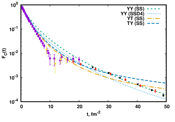
Figure 1: Static approximation for the charge form factor of ³He as a function of $t$ for the rank-one separable Yamaguchi and Tabakin potentials. The experimental data from [35] are denoted by boxes, from [36] are denoted by circles, from [1] are denoted by triangles-up, from  [2] are denoted by triangles-down.

Figure 1 shows the static approximation for different rank-one separable Yamaguchi and Tabakin potentials for the ${}^{3}{\rm He}$ charge form factor as a function of the momentum transfer squared $t$. The line denoted as YY (SS) stands for the ${}^{1}S_{0}$ and ${}^{3}S_{1}$ partial-wave states calculated with the Yamaguchi potential, the lines denoted as YT (SS) and TY (SS) stand for the ${}^{1}S_{0}$ and ${}^{3}S_{1}$ partial-wave states calculated with the Yamaguchi (Y) and Tabakin (T) potentials, respectively. The combinations of the Yamaguchi and Tabakin potentials for $t>40$ fm^-2 give the result that is higher than the experimental data and the result with the Yamaguchi kernel.

The line denoted as YY (SSD4) stands for the ${}^{1}S_{0}$, ${}^{3}S_{1}$ and ${}^{3}D_{1}$ partial-wave states with $p_{D}=4\%$ calculated with the Yamaguchi potential. The contributions of the $P$ and $D$ partial-wave state amplitudes were estimated by using the formulae for C and D (5), and the result was found to be negligible. An additional term in the function $\tau$, which corresponds to the ${}^{3}D_{1}$ partial-wave state was also taken into account and the result was found to be noticeable. Below, the SSD4 notation is used for calculations with the ${}^{1}S_{0}$, ${}^{3}S_{1}$ and ${}^{3}D_{1}$ partial-wave states with $p_{D}=4\%$ where the ${}^{3}D_{1}$ state is taken into account only in function $\tau$. The YY (SSD4) result is less than the YY (SS) one.

The results for $p_{D}=5,6\%$ are very close to $p_{D}=4\%$ and are not plotted. As one can see, all considered rank-one potentials do not give diffraction minima in the form factor $F_{\rm C}$, which exists in the experimental data.

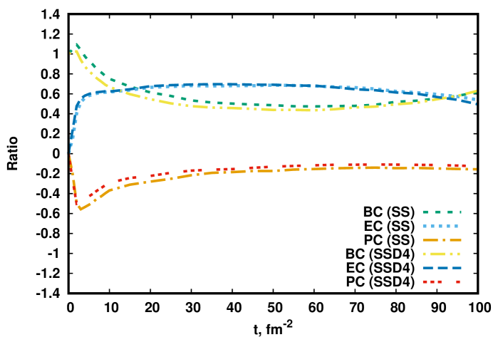
Figure 2: Ratio of the parts of relativistic corrections to their sum as a function of $t$ for the cases SS and SSD4.

Figure 2 shows the ratios of three additive parts of RCs to their sums for two Yamaguchi potentials without (SS) and the ${}^{3}D_{1}$ partial-wave state (SSD4). At high $t$ the contributions are rather flat. One can see that BC and EC are positive while PC is negative and compensate about 20% of BC+EC. For example, for SS calculations at t=50 fm^-2 the EC contribution is about 70%, BC is about 50% and PC is about -20%, at t=100 fm^-2 the EC contribution is about 58%, BC is about 60% and PC is about -18%. The results for SSD4 are very similar especially at high momentum transfer squared.

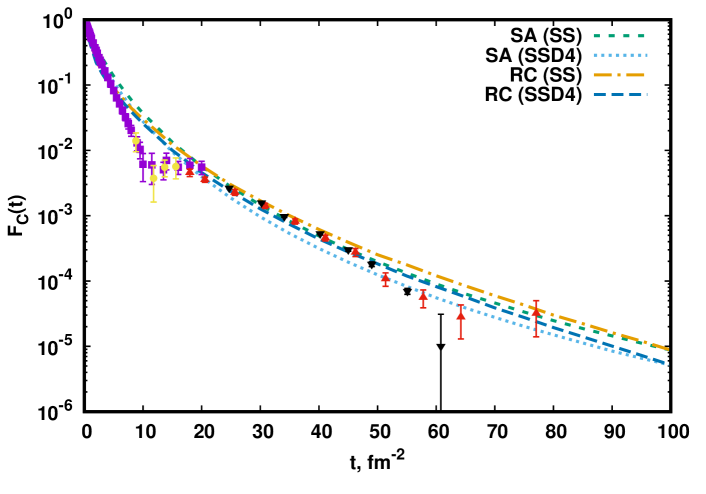
Figure 3: Static approximation and contribution of the relativistic corrections for the charge form factor of ³He as a function of $t$ for the cases SS and SSD4. The experimental data are the same as in Fig. 1.

Figure 3 shows the static approximation and the full relativistic corrections (BC + PC + EC) for two cases: the ${}^{1}S_{0}$, ${}^{3}S_{1}$ (SS) and the ${}^{1}S_{0}$, ${}^{3}S_{1}$ and ${}^{3}D_{1}$ partial-wave states (SSD4). For the SS case RC are higher than SA in the region 20-100 fm^-2 by the maximum factor of 1.3 at t=50 fm^-2. For the SSD4 case RC are higher than SA in the region 15-100 fm^-2 by the maximum factor of 1.5 at t=50 fm^-2.

Taking into account the $D$ wave in the function $\tau$ (SSD4) leads to the result that is less than calculation with only $S$ waves: SA is lower by a factor of 0.7-0.65 at t=20-30 fm^-2 and by a factor of 0.6 at t=50-100 fm^-2, RC is lower by a factor of 0.85-0.8 at t=20-30 fm^-2 and by a factor of 0.7-0.6 at t=50-100 fm^-2.

It should be stressed that neither the inclusion of the ${}^{3}D_{1}$ partial-wave state nor the relativistic corrections lead to zero in the ${}^{3}{\rm He}$ charge form factor. Since the simple rank-one separable kernel considered in the paper does not reproduce the diffraction minima of the form factor $F_{\rm C}$, one need to consider a multirank kernel such as, for example in [19]. In that paper, the first diffraction minimum does appear but at an incorrect momentum transfer. Therefore, one needs to investigate the influence of the relativistic corrections discussed in this paper to the difraction minima position. This work is in progress. However, other effects such as relativistic interaction currents, the off-shell behaviour of the EM nucleon form factors and the precise fitting of the separable functions of the NN interaction can contribute as well.

5 Summary

In this paper, solutions of the BSF equation for ${}^{3}{\rm He}$ have been used to calculate the charge form factor. Expressions for the form factor were obtained by a straightforward relativistic generalization of nonrelativistic expressions. Multiple integration was performed by means of the Monte Carlo algorithm. Moreover, in the calculations, the Lorentz transformation of the arguments of the propagator and the final ${}^{3}{\rm He}$ wave function were taken into account.

Solutions with rank-one Yamaguchi potentials not only with $S$ two-nucleon partial-wave states but also with $P$ and $D$ partial-wave states were taken into account. The only inclusion of the $D$ wave into the function $\tau$ was found to be noticeable while the contributions of the $P$ and $D$ waves by means of the amplitudes were found to be negligible.

Two approximations have been considered: static approximation and relativistic corrections. It was found that the main contribution to the corrections came from the Lorentz boost of the final ${}^{3}{\rm He}$ wave function arguments. At high momentum transfer squared, the relativistic corrections play a significant role and are larger than the static approximation by a factor 1.3-1.5.

References

- [1] R. Arnold, et al., Elastic electron Scattering from He-3 and He-4 at High Momentum Transfer, Phys. Rev. Lett. 40 (1978) 1429. doi:10.1103/PhysRevLett.40.1429.
- [2] A. Camsonne, et al., JLab Measurements of the 3He Form Factors at Large Momentum Transfers, Phys. Rev. Lett. 119 (16) (2017) 162501, [Addendum: Phys.Rev.Lett. 119, 209901 (2017)]. arXiv:1610.07456, doi:10.1103/PhysRevLett.119.162501.
- [3] E. Salpeter, H. Bethe, A Relativistic equation for bound state problems, Phys. Rev. 84 (1951) 1232–1242. doi:10.1103/PhysRev.84.1232.
- [4] J. Tjon, M. Zuilhof, Electromagnetic Properties of the Deuteron in a Relativistic One Boson Exchange Model, Phys. Lett. B 84 (1979) 31–34. doi:10.1016/0370-2693(79)90642-7.
- [5] M. Zuilhof, J. Tjon, Electromagnetic Properties of the Deuteron and the Bethe-Salpeter Equation with One Boson Exchange, Phys. Rev. C 22 (1980) 2369–2382. doi:10.1103/PhysRevC.22.2369.
- [6] E. Hummel, J. Tjon, Relativistic One Boson Exchange Model and Elastic Electron Deuteron Scattering at High Momentum Transfer, Phys. Rev. Lett. 63 (1989) 1788–1791. doi:10.1103/PhysRevLett.63.1788.
- [7] E. Hummel, J. Tjon, Relativistic analysis of meson exchange currents in elastic electron deuteron scattering, Phys. Rev. C 42 (1990) 423–437. doi:10.1103/PhysRevC.42.423.
- [8] E. Hummel, J. Tjon, Relativistic description of electron scattering on the deuteron, Phys. Rev. C 49 (1994) 21–39. arXiv:nucl-th/9309004, doi:10.1103/PhysRevC.49.21.
- [9] L. Marcucci, F. Gross, M. Pena, M. Piarulli, R. Schiavilla, I. Sick, A. Stadler, J. Van Orden, M. Viviani, Electromagnetic Structure of Few-Nucleon Ground States, J. Phys. G 43 (2016) 023002. arXiv:1504.05063, doi:10.1088/0954-3899/43/2/023002.
- [10] G. Rupp, J. Tjon, Relativistic Contributions to the Deuteron Electromagnetic Form-factors, Phys. Rev. C 41 (1990) 472. doi:10.1103/PhysRevC.41.472.
- [11] G. Rupp, L. Streit, J. Tjon, Three Nucleon Bound State Collapse With Tabakin Potentials, Phys. Rev. C 31 (1985) 2285. doi:10.1103/PhysRevC.31.2285.
- [12] S. Bondarenko, V. Burov, S. Dorkin, Sensitivity of polarization observables in elastic e d scattering to the neutron form-factors, Phys. Atom. Nucl. 63 (2000) 774–781. doi:10.1134/1.855706.
- [13] S. Bondarenko, V. Burov, A. Molochkov, G. Smirnov, H. Toki, Bethe-Salpeter approach with the separable interaction for the deuteron, Prog. Part. Nucl. Phys. 48 (2002) 449–535. arXiv:nucl-th/0203069, doi:10.1016/S0146-6410(02)00142-4.
- [14] A. Bekzhanov, S. Bondarenko, V. Burov, Elastic electron-deuteron scattering with modified dipole fit, Nucl. Phys. B Proc. Suppl. 245 (2013) 65–68. doi:10.1016/j.nuclphysbps.2013.10.013.
- [15] A. Bekzhanov, S. Bondarenko, V. Burov, Nucleon form factors for the elastic electron-deuteron scattering at high momentum transfer, JETP Lett. 99 (2014) 613–618. arXiv:1403.4422, doi:10.1134/S0021364014110034.
- [16] L. Faddeev, Scattering theory for a three particle system, Sov. Phys. JETP 12 (1961) 1014–1019.
- [17] A. G. Sitenko and V. F. Kharchenko, Bound states and scattering in a system of three particles, Soviet Physics Uspekhi 14 (1971) 125–153. doi:{10.1070/pu1971v014n02abeh004454}.
- [18] G. Rupp, J. Tjon, Bethe-Salpeter Calculation of Three Nucleon Observables With Rank One Separable Potentials, Phys. Rev. C 37 (1988) 1729. doi:10.1103/PhysRevC.37.1729.
- [19] G. Rupp, J. Tjon, Bethe-Salpeter calculation of three nucleon observables with multirank separable interactions, Phys. Rev. C 45 (1992) 2133. doi:10.1103/PhysRevC.45.2133.
- [20] S. Bondarenko, V. Burov, S. Yurev, Relativistic three-nucleon calculations within the Bethe-Salpeter approach, EPJ Web Conf. 108 (2016) 02015. arXiv:1509.06211, doi:10.1051/epjconf/201610802015.
- [21] S. Bondarenko, V. Burov, S. Yurev, On the relativistic 3D1 partial-wave contribution to the bound three-nucleon system, EPJ Web Conf. 138 (2017) 06003. doi:10.1051/epjconf/201713806003.
- [22] S. Bondarenko, V. Burov, S. Yurev, On the contribution of the P and D partial-wave states to the binding energy of the triton in the Bethe-Salpeter-Faddeev approach, Phys. Atom. Nucl. 82 (1) (2019) 44–49. arXiv:1809.03271, doi:10.1134/S1063778819010058.
- [23] A. Stadler, F. Gross, Relativistic calculation of the triton binding energy and its implications, Phys. Rev. Lett. 78 (1997) 26–29. arXiv:nucl-th/9607012, doi:10.1103/PhysRevLett.78.26.
- [24] A. Stadler, F. Gross, M. Frank, Covariant equations for the three-body bound state, Phys. Rev. C 56 (1997) 2396. arXiv:nucl-th/9703043, doi:10.1103/PhysRevC.56.2396.
- [25] J. Carlson, V. Pandharipande, R. Schiavilla, Variational Monte Carlo calculations of H-3 and He-4 with a relativistic Hamiltonian, Phys. Rev. C 47 (1993) 484–497. doi:10.1103/PhysRevC.47.484.
- [26] S. Bondarenko, V. Burov, S. Yurev, The Rank-One Separable Interaction Kernel for Nucleons with Scalar Propagator, Phys. Part. Nucl. Lett. 15 (4) (2018) 417–421. arXiv:1711.03781, doi:10.1134/S1547477118040052.
- [27] Y. Yamaguchi, Two nucleon problem when the potential is nonlocal but separable. 1., Phys. Rev. 95 (1954) 1628–1634. doi:10.1103/PhysRev.95.1628.
- [28] Y. Yamaguchi, Y. Yamaguchi, Two Nucleon Problem When the Potential Is Nonlocal but Separable. 2, Phys. Rev. 95 (1954) 1635–1643. doi:10.1103/PhysRev.95.1635.
- [29] E. Ydrefors, J. Alvarenga Nogueira, V. Karmanov, T. Frederico, Solving the three-body bound-state Bethe-Salpeter equation in Minkowski space, Phys. Lett. B 791 (2019) 276–280. arXiv:1903.01741, doi:10.1016/j.physletb.2019.02.046.
- [30] E. Ydrefors, J. Alvarenga Nogueira, V. Karmanov, T. Frederico, Three-boson bound states in Minkowski space with contact interactions, Phys. Rev. D 101 (9) (2020) 096018. arXiv:2005.07943, doi:10.1103/PhysRevD.101.096018.
- [31] F. Gross, A. Stadler, M. Pena, Electromagnetic interactions of three body systems in the covariant spectator theory, Phys. Rev. C 69 (2004) 034007. arXiv:nucl-th/0311095, doi:10.1103/PhysRevC.69.034007.
- [32] S. A. Pinto, A. Stadler, F. Gross, Covariant spectator theory for the electromagnetic three-nucleon form factors: Complete impulse approximation, Phys. Rev. C 79 (2009) 054006. arXiv:0901.4313, doi:10.1103/PhysRevC.79.054006.
- [33] S. A. Pinto, A. Stadler, F. Gross, First results for electromagnetic three-nucleon form factors from high-precision two-nucleon interactions, Phys. Rev. C 81 (2010) 014007. arXiv:0911.1473, doi:10.1103/PhysRevC.81.014007.
- [34] S. Bondarenko, V. Burov, S. Yurev, Sensitivity of elastic electron scattering off the 3He to the nucleon form factors, EPJ Web Conf. 204 (2019) 05009. arXiv:1903.01771, doi:10.1051/epjconf/201920405009.
- [35] J. Mccarthy, I. Sick, R. Whitney, Electromagnetic Structure of the Helium Isotopes, Phys. Rev. C 15 (1977) 1396–1414. doi:10.1103/PhysRevC.15.1396.
- [36] M. Bernheim, D. Blum, W. Mcgill, R. Riskalla, C. Trail, T. Stovall, D. Vinciguerra, Elastic electron scattering from he-3 at high momentum transfer, Lett. Nuovo Cim. 5S2 (1972) 431–434. doi:10.1007/BF02905269.
- [37] L. Schiff, Theory of the Electromagnetic Form Factors of H-3 and He-3, Phys. Rev. 133 (1964) B802–B812. doi:10.1103/PhysRev.133.B802.
- [38] B. Gibson, L. Schiff, P- and D-State Contributions to the Charge Form Factors of H-3 and He-3, Phys. Rev. 138 (1965) B26–B32. doi:10.1103/PhysRev.138.B26.