How do Offline Measures for Exploration in Reinforcement Learning behave?

Abstract

Sufficient exploration is paramount for the success of a reinforcement learning agent. Yet, exploration is rarely assessed in an algorithm-independent way. We compare the behavior of three data-based, offline exploration metrics described in the literature on intuitive simple distributions and highlight problems to be aware of when using them. We propose a fourth metric, uniform relative entropy, and implement it using either a k-nearest-neighbor or a nearest-neighbor-ratio estimator, highlighting that the implementation choices have a profound impact on these measures.

1 Introduction

The problem of exploration vs. exploitation is one of the major challenges in reinforcement learning: Should an agent choose actions that maximize its reward (exploitation) or should it choose actions that increase its knowledge while risking lower rewards (exploration)?

Since the agent learns from the data it generates, its ability to generate useful data limits its ability to achieve good performance – that is, if the agent explores insufficiently it will not be able to learn a well-performing policy.

For distinct, given policies $\pi_{i}$ and $\pi_{j}$ on a given task the exploitation is easy to judge: it is the expected return when the actions are chosen according to $\pi_{i}$ or $\pi_{j}$ respectively. The exploration is usually assessed only indirectly in terms of whether the learned policy achieves good returns. An accurate quantification of the exploration can indicate whether the agent is stuck in a local optimum and whether further exploration could improve its performance.

Some algorithms (e.g. tangExplorationStudyCountBased2017 (8, 5, 3, 7)) assess exploration approximately by novelty or uncertainty measures. However, since those algorithms directly try to optimize these measures and these measures are algorithm-specific, it is difficult to use them to compare exploration across algorithms. While the ultimate goal of a reinforcement learning algorithm is to find policies that achieve the highest reward (and eventually purely exploit), achieving this is only possible if the algorithm explores sufficiently and thereby collects the data to find admissible, high-reward solutions. Thus measuring exploration could help in understanding the reason for an algorithm’s performance and can also enable us to select, tune and debug them. This eventually will lead to better-performing reinforcement learning methods.

During early training, with little information on the maximally achievable reward or sparse reward signals, exploration should be high to find these highly-rewarding regions in the state space. Then the algorithm should start to explore around the regions that have proven valuable and gradually shift towards exploitation, while maintaining enough exploration for robust learning, as it moves closer to the optimal solution.

In this work we propose to view the learning process of an RL agent as a data-generating process and assess the achieved exploration offline through the generated data $\mathcal{D}$, since this also allows comparison across algorithms after the training has completed.

Without loss of generality, it is sufficient for the agent to reach highly-rewarding regions in the state space. Note that if the reward function depends on more than the current state, the state can be augmented to include this information. We make no further assumptions on where these highly-rewarding regions are.

We analyze three metrics from the literature (bin-count $X_{\text{bin}}$ glassmanQuadraticRegulatorbasedHeuristic2010 (4), bounding-box-mean $X_{\text{BBM}}$ zhanTakingScenicRoute2019 (11), nuclear-norm $X_{\text{NN}}$ zhanTakingScenicRoute2019 (11)) on four intuitive state distributions. We highlight misleading results of these existing metrics and propose our own metric $\operatorname{X}_{\mathcal{U}\text{rel}}$ that outperforms these existing metrics and provides a more accurate measure of exploration.

In our proposed metric we assume a uniform prior $\mathcal{U}$ on the data generation for theoretically-maximal exploration, and judge the achieved exploration of a collected dataset $\mathcal{D}$ by the negative distance between this prior distribution and the generated data distribution $\mathcal{Q}_{\mathcal{D}}$. This is our uniform-relative-entropy metric

$$\operatorname{X}_{\mathcal{U}\text{rel}}(\mathcal{D})=-D_{\textrm{KL}}\big{(}\mathcal{U}||\mathcal{Q}_{\mathcal{D}}\big{)}-D_{\textrm{KL}}\big{(}\mathcal{Q}_{\mathcal{D}}||\mathcal{U}\big{)}.$$ (1)

2 Method

The learning process of an RL algorithm can be viewed as a data-generating process that is run to produce a dataset of size $n$ sampled from an unknown or implicit distribution $\mathcal{Q}_{\mathcal{D}}$:

$$\mathcal{D}^{(n)}\sim\mathcal{Q}_{\mathcal{D}}:\mathcal{D}^{(n)}=\{(s,a,r,s^{\prime}),\ldots\}$$

where $(s,a,r,s^{\prime})$ denotes a state, action, reward and subsequent state tuple. Repeating the training process again draws a new sample from this process. We assume that the state space of the system forms a (hyper)box, i.e. the state-space $S\in\mathbb{R}^{d}$ and is bounded by lower and upper limits: $\forall s_{i}\in S:s_{l}\leq s_{i}\leq s_{h}$.

In such a case, the maximum-entropy distribution over the state space is a uniform distribution $\mathcal{U}$ udwadiaResultsMaximumEntropy1989 (10). We therefore make the assumption that the highest exploration would be achieved if the explored/generated data follows this uniform distribution and measure this by the uniform relative entropy $\operatorname{X}_{\mathcal{U}\text{rel}}$ (1). In general, the relative-entropy (KL-divergence) term $D_{\textrm{KL}}\big{(}P||Q\big{)}$ requires calculating a usually-intractable integral, which has to be approximated by a sample estimate:

$$D_{\textrm{KL}}\big{(}P||Q\big{)}:= \int p(s)\log\frac{p(s)}{q(s)}ds$$ (2)

$$\approx \sum_{s\sim p}\log\frac{p(s)}{q(s)}$$ (3)

Since the data distribution $\mathcal{Q}_{\mathcal{D}}$ in (1) is not available in closed form, the distance $D_{\textrm{KL}}(\mathcal{U}||\mathcal{Q}_{\mathcal{D}})$ has to be estimated from the available sample $\mathcal{D}$. We assume that we can sample from the prior and that log-likelihood values under the prior are available for these samples. Thus, the KL-divergence can be calculated using a density estimate of $\mathcal{D}$. This corresponds to replacing $p(s)$ and $q(s)$ in (3) by density estimates as necessary.

We looked at two ways of estimating the divergence: a) using an estimate for the density $\hat{q}(s)$ of $\mathcal{Q}_{\mathcal{D}}$ and b) directly estimating the divergence using the ratio $\hat{\rho}(s)$, where $\rho(s)$ is the ratio between $p(s)$ and $q(s)$. These will be described in the following two sections respectively.

We found that the estimators described in the next section underestimate the divergence $D_{\textrm{KL}}\big{(}P||Q\big{)}$ when $P$ is significantly more peaked than $Q$. Since we do not know apriori whether $P$ or $Q$ will be more peaked, choosing either one could lead to an inaccurate estimate in general. However, we found that using the estimators for the symmetric KL-divergence compensates for this problem and follows the actual KL-divergence, i.e. when $p(s)$ and $q(s)$ are known, more closely.

2.1 kNN estimator

One possible estimator for $\hat{q}(s)$ is a k-Nearest-Neighbor (kNN) density estimator bishopPatternRecognition2006 (2), where $V_{d}$ denotes the unit volume of a $d$-dimensional sphere, $R_{k}(x)$ is the Euclidean distance to the $k$-th neighbor of $x$, and $n$ is the total number of samples in $\mathcal{D}$:

$$V_{d}= \frac{\pi^{d/2}}{\Gamma({\frac{d}{2}+1})}$$ (4)

$$\hat{q}_{k}(x)= \frac{k}{n}\frac{1}{V_{d}R_{k}(x)^{d}}=\frac{k}{nV_{d}}\frac{1}{R_{k}(x)^{d}}$$ (5)

where $\Gamma$ denotes the gamma-function.

2.2 NNR estimator

Noshad et al. noshadDirectEstimationInformation2017 (6) proposed an $f$-divergence estimator, the Nearest-Neighbor-Ratio (NNR) estimator, based on the ratio of the nearest neighbors around a query point, which we will use to estimate the KL-divergence.

They state that this estimator has a couple of beneficial properties. Among these, the most important property for our metric is not being affected by the over- / under-estimation artifacts of the kNN estimator close to the boundaries of the state space.

For the general case of estimating $D_{\textrm{KL}}\big{(}P||Q\big{)}$, we take samples from $X\sim Q$ and $Y\sim P$. Let $\mathcal{R}_{k}(Y_{i})$ denote the set of the $k$-nearest neighbors of $Y_{i}$ in the set $Z:=X\cup Y$. $N_{i}$ is the number of points from $X\cap\mathcal{R}_{k}(Y_{i})$, $M_{i}$ is the number of points from $Y\cap\mathcal{R}_{k}(Y_{i})$, $M$ is the number of points in $Y$ and $N$ is the number of points in $X$, $\eta=\frac{M}{N}$, and $C_{L}$ and $C_{U}$ are the lower and upper limits of the densities $P$ and $Q$. Then,

$$D_{\textrm{KL}}(P||Q)\approx \hat{D}_{g}(X,Y)$$ (6)

$$\hat{D}_{g}(X,Y):= \max\left(\frac{1}{M}\sum_{i=1}^{M}\tilde{g}\big{(}\frac{\eta N_{i}}{M_{i}+1},0\big{)}\right)$$ (7)

$$\hat{g}(x):= \max\big{(}g(x),g(C_{L}/C_{U})\big{)}$$ (8)

$$g(\rho):= -\log(\rho)$$ (9)

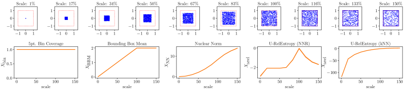
(a) Growing Uniform distribution with values exceeding the state space clipped to the boundaries, thus an increasing number of points on the state-space boundaries for larger scales.

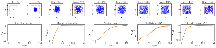
(b) Growing Scale of Truncated Normal

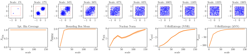
(c) Growing scale of 2-Mixture of Truncated Normal

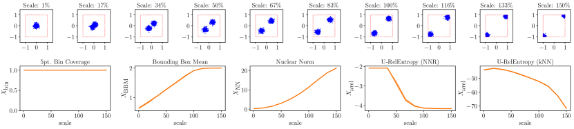
(d) Growing Distance of Modes of 2-Mixture of Truncated Normal

Figure 1: Comparison of exploration metrics on different data generating distributions dependent on one scale parameter: $25$ dimensional factorial distributions, similarly distributed along each dimension. The scatter plots depict first vs. second dimension (top a-d). Each comparison (bottom) shows the different exploration metrics $X_{\text{bin}},X_{\text{BBM}},X_{\text{NN}}$ and $\operatorname{X}_{\mathcal{U}\text{rel}}$ (ours) on the $y$ axis and the scale parameter is depicted on the $x$ axis.

3 Related Work

Exploration can be measured by dividing the state space into equally spaced bins and counting the percentage of non-empty bins glassmanQuadraticRegulatorbasedHeuristic2010 (4). This is related to the directed count-based exploration metric in discrete reinforcement-learning settings thrunEfficientExplorationReinforcement1992 (9, 1) where each visited state acquires a bonus, for example $\sum_{i}^{n}\sqrt{i}$ when it has been visited $n$ times. Thus, visiting all states equally often in the limit achieves the highest exploration bonus. This has also been extended to continuous domains by using locality-sensitive hashing to discretize the state space tangExplorationStudyCountBased2017 (8). We will compare our metric $\operatorname{X}_{\mathcal{U}\text{rel}}$ against this ratio of visited bins $X_{\text{bin}}$. We choose the divisions such that we expect five data points in each bin on average in the uniform case: $\mathrm{divisions}=\left\lceil\left(\frac{N}{5}\right)^{\frac{1}{d}}\right\rceil$. Since we round up, the number of bins can exceed the total number of points $N$, to compensate we scale the ratio by $\frac{1}{\min(N,\mathrm{divisions}})$ such that in the case of more boxes than points the metric reaches its maximum when all points lie in different boxes.

Zhan et al. zhanTakingScenicRoute2019 (11) propose to measure the sum of the side lengths of the hyperbox enclosing the collected data $\mathcal{D}$ parallel to the state-space coordinate system, and they denote this as the bounding-box-sum metric. To reduce the impact of the state-space dimensionality, we use the mean instead of the sum of the bounding box side lengths and denote this as the $X_{\text{BBM}}$ metric.

By its definition this metric is prone to over-estimating the covered state space if the collected data points are not aligned with the axes. So the authors zhanTakingScenicRoute2019 (11) took this problem into account and derived the nuclear-norm metric $X_{\text{NN}}$ based on the sum of the eigenvalues (the trace) of the estimated covariance $\mathbf{\hat{C}}$ of the data: $X_{\text{NN}}(\mathcal{D}):=\operatorname{\bf trace}\big{(}\mathbf{\hat{C}}(\mathcal{D})\big{)}$.

4 Evaluation

To compare the different exploration metrics, we assumed a $d=25$-dimensional state space, generated data from four different types of distributions, and compared the exploration metrics on these data. The experiments were repeated $10$ times, and the mean and min-max values are plotted.

These four cases are depicted in Figure 1. While the data are $d$-dimensional, they come from factorial distributions, similarly distributed along each dimension. Thus, we can gain intuition about the distribution from scatter plots of the first vs. second dimension. This is depicted at the top of each of the four parts. The bottom part of each comparison shows the different exploration metrics, where the scale parameter is depicted on the $x$ axis and the exploration measure on the $y$ axis.

(a) Growing Uniform:

Figure 1(a) depicts data generated by a uniform distribution, centered around the middle of the state space, with minimal and maximal values growing relatively to the full state space according to the scale parameter from $1\%$ to $150\%$. Since in the latter case, many points would lie outside the allowed state space; these values are clipped to the state space boundaries. This loosely corresponds to an undirectedly exploring agent that overshoots and hits the state space limits, sliding along the state-space boundaries. Note how the estimation (kNN vs. NNR) has a great impact on the $\operatorname{X}_{\mathcal{U}\text{rel}}$ metric’s performance here: We would expect a maximum around a scale of $100\%$ and smaller values before and after (due to clipping). Here the $\operatorname{X}_{\mathcal{U}\text{rel}}$ (NNR) metric most closely follows this expectation. The true diverge would follow a similar shape although with more extreme values.

(b) Truncated Normal:

Figure 1(b) depicts data of a truncated Gaussian distribution with the mean in the center of the state-space box and the scale across all dimensions set equal to the scale parameter. This example is inspired by random exploration around a centered starting point. Since the distribution is truncated, increasing the scale leads to more and more uniform outcomes. The true divergence would converge to zero, which is appropriately reflected in the metrics. The only difference to the true divergence is that it again would exhibit more extreme low values and rise more steeply. If an untruncated Gaussian distribution with clipping was used, we would expect to see effects similar to Figure 1(a).

(c) Bi-Modal Truncated Normal growing scale:

Figure 1(c) shows a mixture of two truncated Gaussian distributions, spaced symmetrically around the center of the state space, with growing standard deviations set equal to the scale parameter. This can be compared to cases where the search process is initiated from certain fixed starting positions. Increasing the scale again leads to more and more uniform behavior. Note that the bounding-box mean $X_{\text{BBM}}$ rapidly approaches the maximum value and provides no further information. A further interesting artifact is visible in the nuclear norm $X_{\text{NN}}$, where the measured exploration drops without an intuitive explanation.

(d) Bi-Modal Truncated Normal moving locations:

Figure 1(d) shows a mixture of two truncated Gaussian distributions, with equal standard deviations but located further and further apart (depending on the scale parameter). In this case, the state space coverage should increase until both distributions are sufficiently apart, should then stay the same, and begin to drop as the proximity to the state space limits the points to an ever smaller volume. While somewhat contrived, it highlights difficulties in the exploration metrics. Both the bounding-box mean $X_{\text{BBM}}$ and the nuclear norm $X_{\text{NN}}$ completely fail to account for vastly unexplored areas between the extreme points. Since the $\operatorname{X}_{\mathcal{U}\text{rel}}$ NNR metric is clipped (by definition of NNR) the metric reaches its limits when the density ratios become extreme, which presumably happens for very small and large scale parameters in this setting. Here the $X_{\text{Urel}}$ kNN appears to outperform NNR even though it also suffers from under-estimation of the divergence for points close to the boundaries.

5 Conclusion

We compared four exploration metrics on generated data and highlighted shortcomings and caveats of these metrics: (i) Our $\operatorname{X}_{\mathcal{U}\text{rel}}$-NNR metric correctly shows a decrease in exploration when points are clipped to the state space boundaries, whereas the other metrics do not detect this problem, (ii) $\operatorname{X}_{\mathcal{U}\text{rel}}$converges to zero as the state space coverage becomes more uniform as shown for the growing truncated normal distributions, (iii) while $X_{\text{bin}}$ is shown not to be useful in high-dimensions, $\operatorname{X}_{\mathcal{U}\text{rel}}$ is. (iv) $X_{\text{BBM}}$rapidly reaches the maximum and does not provide any useful information and $X_{\text{NN}}$ over-estimates the importance of the most spread out points. We propose our metric using the uniform distribution $\mathcal{U}$ as the most general case. However, in some cases more information about the task may be available. For example, when a rough estimate of the goal location is already known, then it is more reasonable to explore around that location, rather than uniformly over the whole state space. In such a case a more appropriate prior should be selected.

These metrics could also be used for goal babbling: consider a redundant robot arm, where the relevant aspect would be the reached configurations of the end-effector rather than reaching all possible joint-space configurations. In this case, transforming the collected data into the goal space, i.e. the end-effector configurations, and estimating the metrics in that space would provide an effective measurement of exploration.

We showed that the choice of metric, as well as the implementation details (such as the kNN vs. NNR estimator) greatly influence the behavior of the metric, and that, since approximations are necessary, an intuitive understanding of the metrics is beneficial.

Our metric is designed to be used offline, to provide information about the exploration performance across algorithms. This allows us to approximate the relative entropy more accurately than would be possible inside the training loop.

In future work we will use this metric to analyze the learning progress of various deep reinforcement learning algorithms. We will also investigate whether this can help detect why learning sometimes fails.

References

- (1) Marc Bellemare et al. “Unifying Count-Based Exploration and Intrinsic Motivation” In Advances in Neural Information Processing Systems, 2016, pp. 1471–1479
- (2) Christopher M. Bishop “Pattern Recognition” In Machine Learning 128, 2006, pp. 1–58
- (3) Yuri Burda, Harrison Edwards, Amos J. Storkey and Oleg Klimov “Exploration by Random Network Distillation” In 7th International Conference on Learning Representations, ICLR, 2019
- (4) Elena Glassman and Russ Tedrake “A Quadratic Regulator-Based Heuristic for Rapidly Exploring State Space” In 2010 IEEE Int. Conf. Robotics and Automation (ICRA) IEEE, 2010
- (5) Zhang-Wei Hong et al. “Diversity-Driven Exploration Strategy for Deep Reinforcement Learning” In Advances in Neural Information Processing Systems, 2018, pp. 10489–10500
- (6) Morteza Noshad, Kevin R. Moon, Salimeh Yasaei Sekeh and Alfred O. Hero “Direct Estimation of Information Divergence Using Nearest Neighbor Ratios” In 2017 IEEE International Symposium on Information Theory (ISIT), 2017, pp. 903–907 DOI: 10.1109/ISIT.2017.8006659
- (7) Vitchyr H. Pong et al. “Skew-Fit: State-Covering Self-Supervised Reinforcement Learning”, 2020 arXiv:1903.03698
- (8) Haoran Tang et al. “#Exploration: A Study of Count-Based Exploration for Deep Reinforcement Learning” In Advances in Neural Information Processing Systems 30 Curran Associates, Inc., 2017, pp. 2753–2762
- (9) Sebastian B. Thrun “Efficient Exploration in Reinforcement Learning”, 1992
- (10) Firdaus E. Udwadia “Some Results on Maximum Entropy Distributions for Parameters Known to Lie in Finite Intervals” In Siam Review 31.1 SIAM, 1989, pp. 103–109
- (11) Zeping Zhan, Batu Aytemiz and Adam M Smith “Taking the Scenic Route: Automatic Exploration for Videogames” In KEG@ AAAI, 2019