Information-disturbance trade-off in generalized entanglement swapping

Abstract

We study information-disturbance trade-off in generalized entanglement swapping protocols wherein starting from Bell pairs $\left(1,2\right)$ and $\left(3,4\right)$, one performs an arbitrary joint measurement on $\left(2,3\right)$, so that $\left(1,4\right)$ now becomes correlated. We obtain trade-off inequalities between information gain in correlations of $\left(1,4\right)$ and residual information in correlations of $\left(1,2\right)$ and $\left(3,4\right)$, respectively, and we argue that information contained in correlations (information) is conserved if each inequality is an equality. We show that information is conserved for a maximally entangled measurement but is not conserved for any other complete orthogonal measurement and Bell measurement mixed with white noise. However, rather surprisingly, we find that information is conserved for rank-2 Bell diagonal measurements, although such measurements do not conserve entanglement. We also show that a separable measurement on $\left(2,3\right)$ can conserve information, even if, as in our example, the post-measurement states of all three pairs $\left(1,2\right)$, $\left(3,4\right)$, and $\left(1,4\right)$ become separable. This implies that correlations from an entangled pair can be transferred to separable pairs in nontrivial ways so that no information is lost in the process.

I Introduction

Quantum systems that have never interacted in the past can nevertheless become entangled via the procedure of entanglement swapping (swapping, ). The basic idea of entanglement swapping is simple and can be illustrated with the following protocol: Alice shares a Bell pair $\left(1,2\right)$ with Bob and Bob shares another Bell pair $\left(3,4\right)$ with Charlie, where all three of them are physically separated; Bob performs Bell measurement on $\left(2,3\right)$ and discloses the outcome to both Alice and Charlie, and as Bob’s measurement projects $\left(2,3\right)$ onto a Bell state, the result is that Alice and Charlie end up with a Bell pair $\left(1,4\right)$ as well.

The protocol just described mimics quantum teleportation of a qubit that is maximally entangled with another qubit, and this is why entanglement swapping is often considered as teleportation of entanglement. The protocol, however, can be generalized in several ways, such as modifying the initial states, Bob’s measurement, or both, where some of the generalizations, as one may note, go beyond that of teleportation of entanglement. Generalized entanglement swapping protocols have been well-studied (e.g., (Bose-1998-swapping-multiparty, ; Gour-Sanders-2004, )) and have found important applications in quantum networks (Perseguers-2008-networks, ; networks-review, ) and quantum nonlocality related problems (swapping-CHSH, ; swapping-activation, ).

A generic feature of all “entanglement swapping” protocols is that at the end of a protocol, the pairs $\left(1,2\right)$ and $\left(3,4\right)$ no longer remain as correlated as they were prior to Bob’s measurement, whereas the pair $\left(1,4\right)$ that was completely uncorrelated earlier becomes correlated. Thus “entanglement swapping” can also be seen as a procedure that, in effect, transfers correlations from entangled pairs to an unentangled pair, where the transfer of correlations is brought about by Bob’s measurement that disturbs the initial states. This suggests some kind of information-disturbance trade-off for Bob’s measurements once we interpret “information” as information contained in correlations of a two-qubit state. In this paper, we make this intuition precise in terms of an information theoretic measure of entanglement (Zeilinger-99, ; BZ-1999, ; BZZ-2001, ). This measure, denoted by $\mathcal{I}\left(\rho\right)$, quantifies the total amount of information contained in correlations of a two-qubit state $\rho$ (often we shall use information as short for “information contained in correlations” when there is no scope for confusion). Our motivation, in part, comes from an earlier work (complementarity, ) on complementarity and information.

Specifically, we consider protocols in which starting from Bell pairs $\left(1,2\right)$ and $\left(3,4\right)$, Bob performs an arbitrary two-qubit measurement on $\left(2,3\right)$, so that $\left(1,4\right)$ now becomes correlated. As the initial states are taken to be maximally entangled, the nonlocal properties of $\left(1,4\right)$ will depend only on Bob’s measurement. This allows us to investigate information-disturbance type trade-off in a particularly clean set-up.

Let us now briefly discuss our results. Let $\mathcal{I}_{ij}^{f}$ denote the information contained in correlations of the pair $\left(i,j\right)$ post Bob’s measurement. We will show that the following inequalities hold:

$$\bar{\mathcal{I}}_{m\,m+1}^{f}+\bar{\mathcal{I}}_{14}^{f} \leq 2,\;m=1,3,$$ (1)

where $\bar{\mathcal{I}}_{14}^{f}$ is the average information gain in correlations of $\left(1,4\right)$, and $\bar{\mathcal{I}}_{m\,m+1}^{f}$ is the average residual information in correlations of the pair $\left(m,m+1\right)$. Here, the first inequality captures the trade-off for the bipartition $A|BC$ and the second for $C|AB$. This is consistent with the observation that $\left(1,4\right)$, in fact, gains correlations at the expense of $\left(1,2\right)$ across $A|BC$, but at the expense of $\left(3,4\right)$ across $C|AB$.

Although in this paper we consider only Bell pairs as initial states, the inequalities (1) are completely general and hold for all choices of two-qubit initial states and Bob’s measurement (see Sec. III for details).

The physical significance of (1) can be understood as follows. For a maximally entangled $\rho$, it holds that $\mathcal{I}\left(\rho\right)=2$ (BZ-1999, ), so we can write (1) as

$$\bar{\mathcal{I}}_{m\,m+1}^{f}+\bar{\mathcal{I}}_{14}^{f} \leq \mathcal{I}_{m\,m+1}^{i},\;m=1,3,$$ (2)

where $\mathcal{I}_{m\,m+1}^{i}$ denotes information contained in correlations of the pair $\left(m,m+1\right)$ prior to Bob’s measurement. Now we have a clear physical interpretation of (1): If equality holds, then no information flows out of the system and the amount of information gained in $\left(1,4\right)$ is exactly equal to the amount of information lost in $\left(m,m+1\right)$ for $m=1,3$. On the other hand, if any of them is strict then there is loss of information. Thus, information is conserved across the bipartitions $A|BC$ and $C|AB$ iff equality holds in (1).

Naturally, the question is, which measurements conserve information in our protocols? It is easy to see information is conserved for maximally entangled measurements, such as Bell measurement. But are there other measurements with the same property? In particular, are there measurements that conserve information but not entanglement? Intuitively, it appears that only maximally entangled measurements would conserve information, and other measurements would necessarily lead to information loss. We find that this is indeed the case for all complete orthogonal (but not maximally entangled) measurements and Bell measurement mixed with white noise. But surprisingly, it turns out there are exceptions: in particular, rank-2 Bell-diagonal measurements conserve information over all intermediate strengths. Interestingly, information is conserved even when they are separable, and all post-measurement states become separable after Bob’s measurement. The latter suggests that separable measurements can distribute correlations from an entangled pair to separable pairs in ways such that information is conserved.

Here we want to emphasize that we are able to express (1) in the form of (2) only because the initial states are maximally entangled. In this case, we can infer that information can never be increased post Bob’s measurement and classical communication of the measurement outcome. However, if the initial states are not maximally entangled, one has $\mathcal{I}_{m\,m+1}^{i}<2$ for $m=1,3$, and in such cases (2) does not follow from (1) because $\mathcal{I}$ is not a LOCC (Local Operations and Classical Communication) monotone (I-not-monotone, ). However, as noted earlier, the inequalities (1) must always hold in all entanglement swapping protocols, hence they are of basic importance.

The paper is organized as follows. In Sec. II, we discuss the basics of the entanglement swapping protocol considered in this paper. Here we show that the post-measurement state of $\left(1,4\right)$ for any given outcome is completely specified in terms of the corresponding POVM element; however, similar expressions for $\left(1,2\right)$ and $\left(3,4\right)$ could not be obtained for they do not seem to have any simplified form in general, though it is clear they depend only on the POVM elements, as expected. Next we consider a general family of Bell-diagonal measurements and obtain the post-measurement states for all three pairs $\left(1,4\right)$, $\left(1,2\right)$, and $\left(3,4\right)$. In Sec. III, we obtain the trade-off relations (1). We study the trade-off relations for complete orthogonal measurements and Bell-diagonal measurements in Sec. IV. We conclude with a brief summary of the paper and a short discussion on open questions in Sec. V.

II generalized protocol

In this section, we first study how the initial Bell states transform under Bob’s two-qubit measurement $\bm{\Pi}$ (a POVM) and obtain an expression for the post-measurement state of $\left(1,4\right)$. After that, we consider a family of Bell-diagonal measurements and obtain expressions for the post-measurement states for all three pairs. These expressions will be used to analyze the trade-off relations for specific measurements in Section IV.

To begin with, Alice and Charlie each shares a Bell state $\left|\Psi_{1}\right\rangle$ with Bob, where $\left|\Psi_{1}\right\rangle$ belongs to the two-qubit Bell basis

$$\left|\Psi_{1}\right\rangle=\frac{1}{\sqrt{2}}\left(\left|00\right\rangle+\left|11\right\rangle\right); \left|\Psi_{2}\right\rangle=\frac{1}{\sqrt{2}}\left(\left|00\right\rangle-\left|11\right\rangle\right);$$

$$\left|\Psi_{3}\right\rangle=\frac{1}{\sqrt{2}}\left(\left|01\right\rangle+\left|10\right\rangle\right); \left|\Psi_{4}\right\rangle=\frac{1}{\sqrt{2}}\left(\left|01\right\rangle-\left|10\right\rangle\right).$$ (3)

Then, the four-qubit initial state is given by

$$\left|\Phi\right\rangle = \left|\Psi_{1}\right\rangle_{12}\left|\Psi_{1}\right\rangle_{34},$$ (4)

where$\left(1,2\right)$ is shared between Alice and Bob, and $\left(3,4\right)$ is shared between Bob and Charlie.

Bob’s measurement $\bm{\Pi}$ can be specified by a collection of positive semi-definite operators $\Pi_{i}$ satisfying $\sum\Pi_{i}=\mathbb{I}$, where each POVM element admits decomposition of the form

$$\Pi_{k} = \sum_{\alpha=1}^{4}\pi_{k\alpha}\left|\phi_{k\alpha}\right\rangle\left\langle\phi_{k\alpha}\right|,$$ (5)

where $\left|\phi_{k\alpha}\right\rangle$, $\alpha=1,\dots,4$ form a complete orthonormal basis on $\mathbb{C}^{2}\otimes\mathbb{C}^{2}$, $\pi_{k\alpha}\geq 0$ for $\alpha=1,\dots,4$. Note that, if $\Pi_{k}$ is not full-rank, the decomposition (5) is not unique, but as we will see, this will not affect post-measurement states.

The probability of obtaining outcome $k$ is

$$p_{k} = \left\langle\Phi\left|\Pi_{k}\otimes\mathbb{I}\right|\Phi\right\rangle=\frac{1}{4}\mbox{Tr}\Pi_{k}$$ (6)

and the post-measurement four-qubit state is given by

$$\left|\Phi_{k}\right\rangle = \frac{1}{\sqrt{p_{k}}}\sqrt{\Pi_{k}}\otimes\mathbb{I}\left|\Phi\right\rangle,$$ (7)

where it is understood that $\Pi_{k}$ acts on the pair $\left(2,3\right)$ and the identity operator acts on the pair $\left(1,4\right)$.

To find an expression for (7) we proceed as follows. First we write the initial state (4) as

$$\left|\Phi\right\rangle = \frac{1}{2}\sum_{i=1}^{4}\left|\Psi_{i}\right\rangle_{23}\left|\Psi_{i}\right\rangle_{14}.$$ (8)

We now use the fact that (8) is $U\otimes U^{*}$ invariant and therefore can be written as

$$\left|\Phi\right\rangle = \frac{1}{2}\sum_{\alpha=1}^{4}\left|\phi_{k\alpha}\right\rangle_{23}\left|\phi_{k\alpha}^{*}\right\rangle_{14},$$ (9)

where the complex conjugation is in the computational basis. Then, using (9) and (5) in (7) we get

$$\left|\Phi_{k}\right\rangle = \frac{1}{2\sqrt{p_{k}}}\sum_{\alpha=1}^{4}\sqrt{\pi_{k\alpha}}\left|\phi_{k\alpha}\right\rangle_{23}\left|\phi_{k\alpha}^{*}\right\rangle_{14}.$$ (10)

The above expression will be used to find the post-measurement states.

By tracing out qubits 2 and 3 from (10) we immediately obtain the post-measurement state of $\left(1,4\right)$:

$$\rho_{14|k} = \frac{1}{4p_{k}}\sum_{\alpha=1}^{4}\pi_{k\alpha}\left|\phi_{k\alpha}^{*}\right\rangle\left\langle\phi_{k\alpha}^{*}\right|=\frac{\Pi_{k}^{*}}{\mbox{Tr}\left(\Pi_{k}\right)},$$ (11)

where $\Pi_{k}^{*}=\sum_{\alpha=1}^{4}\pi_{k,\alpha}\left|\phi_{k\alpha}^{*}\right\rangle\left\langle\phi_{k\alpha}^{*}\right|$.

Obtaining similar compact expressions for $\left(1,2\right)$ and $\left(3,4\right)$, however, seems difficult, unless we know more about the measurement itself. So now we turn our attention to Bell-diagonal measurements and show that it is in fact possible to obtain exact expressions for all post-measurement states.

Bell-diagonal measurements

We consider a family of Bell-diagonal measurements $\mathbb{M}\left(\lambda\right)$ characterized by a real variable $\lambda$ ($0\leq\lambda\leq 1$). The POVM elements $\mathbb{M}_{i}\left(\lambda\right)$, $i=1,\dots,4$ are positive semi-definite operators satisfying $\sum_{i}\mathbb{M}_{i}\left(\lambda\right)=\mathbb{I}$ and are given by

$$\mathbb{M}_{i}\left(\lambda\right) = \lambda\left|\Psi_{i}\right\rangle\left\langle\Psi_{i}\right|+\left(1-\lambda\right)\sum_{l=1}^{4}q_{il}\left|\Psi_{l}\right\rangle\left\langle\Psi_{l}\right|,$$ (12)

where for every $i$, $0\leq q_{il}\leq 1$ and $\sum_{i=1}^{4}q_{il}=1$ for every $l=1,\dots,4$. The POVM elements can be explicitly written in the Bell-diagonal form

$$\mathbb{M}_{i}\left(\lambda\right) = x_{i}\left|\Psi_{i}\right\rangle\left\langle\Psi_{i}\right|+\sum_{j\neq i}y_{ij}\left|\Psi_{j}\right\rangle\left\langle\Psi_{j}\right|$$ (13)

for $i,j=1,\dots,4$, where $x_{i}=\left[\lambda+\left(1-\lambda\right)q_{ii}\right]$ and $y_{ij}=\left(1-\lambda\right)q_{ij}$.

The probability of outcome $k$ is obtained from (6):

$$p_{k} = \frac{1}{4}\left(x_{k}+\sum_{j\neq k}y_{kj}\right).$$ (14)

The post-measurement state of $\left(1,4\right)$ is obtained from (11):

$$\rho_{14|k} = \frac{1}{x_{k}+\underset{j\neq k}{\sum}y_{kj}}\mathbb{M}_{k}\left(\lambda\right)$$ (15)

Now we need to find $\rho_{12|k}$ and $\rho_{34|k}$. First we observe that the following identities hold for a four qubit-system:

$$\left|\Psi_{1}\right\rangle_{12}\left|\Psi_{1}\right\rangle_{34} = \frac{1}{2}\sum_{i=1}^{4}\left|\Psi_{i}\right\rangle_{23}\left|\Psi_{i}\right\rangle_{14},$$

$$\left|\Psi_{2}\right\rangle_{12}\left|\Psi_{2}\right\rangle_{34} = \frac{1}{2}\sum_{i=1,2}\left|\Psi_{i}\right\rangle_{23}\left|\Psi_{i}\right\rangle_{14}-\frac{1}{2}\sum_{i=3,4}\left|\Psi_{i}\right\rangle_{23}\left|\Psi_{i}\right\rangle_{14},$$

$$\left|\Psi_{3}\right\rangle_{12}\left|\Psi_{3}\right\rangle_{34} = \frac{1}{2}\sum_{i=1,3}\left|\Psi_{i}\right\rangle_{23}\left|\Psi_{i}\right\rangle_{14}-\frac{1}{2}\sum_{i=2,4}\left|\Psi_{i}\right\rangle_{23}\left|\Psi_{i}\right\rangle_{14},$$

$$\left|\Psi_{4}\right\rangle_{12}\left|\Psi_{4}\right\rangle_{34} = \frac{1}{2}\sum_{i=1,4}\left|\Psi_{i}\right\rangle_{23}\left|\Psi_{i}\right\rangle_{14}-\frac{1}{2}\sum_{i=2,3}\left|\Psi_{i}\right\rangle_{23}\left|\Psi_{i}\right\rangle_{14}.$$

The above identities can be written in a compact form as

$$\left|\Psi_{i}\right\rangle_{12}\left|\Psi_{i}\right\rangle_{34} = \frac{1}{2}\sum_{l=1}^{4}\mu_{il}\left|\Psi_{l}\right\rangle_{23}\left|\Psi_{l}\right\rangle_{14},$$ (16)

where $i=1,\dots,4$, and $\mu_{il}\in\left\{+1,-1\right\}$. Now substituting (13) in (7) and after simplification using (16), we find that

$$\left|\Phi_{k}\right\rangle = \frac{1}{4\sqrt{p_{k}}}\sum_{l=1}^{4}\gamma_{l}\left|\Psi_{l}\right\rangle_{12}\left|\Psi_{l}\right\rangle_{34},$$ (17)

where $\gamma_{l}=\left(\sqrt{x_{k}}\mu_{kl}+\sum_{j\neq k}\sqrt{y_{kj}}\mu_{jl}\right)$ and $p_{k}$ is given by (14). Then the post-measurement states $\rho_{12|k}$ and $\rho_{34|k}$ are given by

$$\rho_{m\,m+1|k} = \sum_{l=1}^{4}\tau_{l}\left|\Psi_{l}\right\rangle\left\langle\Psi_{l}\right|,\;m=1,3,$$ (18)

where $\tau_{l}=\frac{\gamma_{l}^{2}}{16p_{k}}$ for $l=1,\dots,4$. So all post-measurement states are Bell-diagonal.

III Trade-off relations

We begin with the definition of $\mathcal{I}\left(\rho\right)$ – the total information contained in correlations of a two-qubit state $\rho$. It is defined as (BZ-1999, ; BZZ-2001, )

$$\mathcal{I}\left(\rho\right) = \max_{\bm{n},\bm{m}}\left(I_{nn}+I_{mm}\right),$$ (19)

where $I_{kk}=\left[\mbox{Tr}\rho\left(\sigma_{k}\otimes\sigma_{k}\right)\right]^{2}$ for a unit vector $\bm{k}\in\mathbb{R}^{3}$, $\sigma_{n}=\bm{\sigma\cdot n}$, $\sigma_{x}.\sigma_{y},\sigma_{z}$ being the standard Pauli matrices, and the maximum is taken over all pairs $\left(\bm{n},\bm{m}\right)$ of unit vectors with the property that the spin measurements along $\bm{n}$ and along $\bm{m}$ are mutually unbiased.

The following properties hold:

• $\mathcal{I}\left(\rho\right)\leq 2$, where the equality is achieved for maximally entangled states;

• $\mathcal{I}\left(\rho\right)\leq 1$ for separable states;

• $\mathcal{I}\left(\rho\right)=\frac{\mathcal{B}^{2}\left(\rho\right)}{4}$ (BZZ-2001, ; complementarity, ), where $\mathcal{B}\left(\rho\right)$ is the maximal mean value of the Bell-CHSH observable (Horodecki-1995-Bell, ; Horodecki-1996-Bell-2, ).

The last property is particularly important for two reasons. First, it provides us with a computable formula for $\mathcal{I}\left(\rho\right)$ (see next section) and second, it plays a crucial role in the derivation of the trade-off relations. Note however that, though $\mathcal{I}\left(\rho\right)$ and $\mathcal{B}\left(\rho\right)$ are related for any two-qubit state, such a relation may not hold in higher dimensions, and moreover, $\mathcal{I}\left(\rho\right)$ and Bell-CHSH violation are conceptually inequivalent.

The trade-off relations are obtained by exploiting the monogamy property of $\mathcal{I}$. This property follows from the Bell-monogamy (Bell-monogamy, ; Bell-monogamy-2, ): For any three qubit state $\sigma_{abc}$ it holds that

$$\mathcal{B}^{2}\left(\sigma_{ab}\right)+\mathcal{B}^{2}\left(\sigma_{ac}\right) \leq 8,$$ (20)

where $\sigma_{ab}=\mbox{Tr}_{c}\left(\sigma_{abc}\right)$, $\sigma_{ac}=\mbox{Tr}_{b}\left(\sigma_{abc}\right)$. Similar inequalities hold for other possible pairs.

Since $\mathcal{I}\left(\rho\right)=\frac{\mathcal{B}^{2}\left(\rho\right)}{4}$, (20) therefore leads to the $\mathcal{I}$-monogamy inequality

$$\mathcal{I}\left(\sigma_{ab}\right)+\mathcal{I}\left(\sigma_{ac}\right) \leq 2$$ (21)

for any three qubit state $\sigma_{abc}$.

To obtain the trade-off relations (1) we now proceed as follows. Let $\rho_{1234}$ be the four-qubit state post Bob’s measurement and $\rho_{ij}$ be the post-measurement states of the pairs $\left(i,j\right)$ obtained from $\rho_{1234}$ by tracing out the appropriate qubits, e.g. $\rho_{14}=\text{Tr}_{23}\left(\rho_{1234}\right)$ and so on. Then applying (21) to each of the three-qubit states $\rho_{124}=\mbox{Tr}_{3}\left(\rho_{1234}\right)$ and $\rho_{134}=\mbox{Tr}_{2}\left(\rho_{1234}\right)$ we get the following inequalities

$$\mathcal{I}_{m\,m+1}^{f}+\mathcal{I}_{14}^{f} \leq 2,\;m=1,3$$ (22)

that hold for any outcome of Bob’s measurement. Here, $\mathcal{I}_{14}^{f}$ amounts to the gain in information in correlations of $\left(1,4\right)$ as $\mathcal{I}_{14}^{i}=0$ initially, whereas $\mathcal{I}_{m\,m+1}^{f}$ amounts to the residual information contained in correlations of $\left(m,m+1\right)$ for $m=1,3$.

Now, for any given measurement there are three possible scenarios: the inequalities (22) are strict for all outcomes, some outcomes, or none of the outcomes. So one must consider weighted average of (22) taken over all possible outcomes and that gives us the desired relations (1) (reproduced here for convenience)

$$\bar{\mathcal{I}}_{m\,m+1}^{f}+\bar{\mathcal{I}}_{14}^{f} \leq 2,\;m=1,3$$ (23)

where $\overline{\mathcal{I}}$ denotes the weighted average over all outcomes.

As we explained in the introduction, information is conserved across the bipartitions provided equality holds in each of the above inequalities. So now we want to find out which measurements conserve information. In the next section, we present partial answers and some useful insights.

IV trade-off relations for specific measurements

To study the trade-off relations we need to be able to compute $\mathcal{I\left(\rho\right)}$ for any two-qubit $\rho$. Fortunately, it is possible by virtue of the relation $\mathcal{I}\left(\rho\right)=\frac{\mathcal{B}^{2}\left(\rho\right)}{4}$.

Let $t_{11},t_{22},t_{33}$ be the eigenvalues of the real $3\times 3$ matrix $T$, the elements of which are defined as $T_{ij}={\rm Tr}\left[\rho\left(\sigma_{i}\otimes\sigma_{j}\right)\right]$ for $i,j=1,2,3$. Define the function

$$M\left(\rho\right) = \max_{i>j}\left(\left|t_{ii}\right|^{2}+\left|t_{jj}\right|^{2}\right).$$ (24)

Then, $\mathcal{B}\left(\rho\right)=2\sqrt{M\left(\rho\right)}$ (Horodecki-1995-Bell, ) and consequently,

$$\mathcal{I}\left(\rho\right) = M\left(\rho\right).$$ (25)

Complete orthogonal measurements

In a complete orthogonal measurement (COM) $\left\{\Pi_{k}\right\}$, each POVM element $\Pi_{k}$ is a projection operator $\left|\eta_{k}\right\rangle\left\langle\eta_{k}\right|$ that projects the system onto $\left|\eta_{k}\right\rangle$, which is an eigenvector of the measurement, and these eigenvectors $\left\{\left|\eta_{k}\right\rangle\right\}$ form a complete orthonormal basis of the Hilbert space of the system, i.e., $\text{Tr}\Pi_{k}\Pi_{l}=\delta_{kl}$. The simplest example of a COM is the Bell measurement for which (23) are in fact equalities, so information is conserved.

Now consider a COM, which is not maximally entangled. Then at least one of the eigenvectors must be nonmaximally entangled. Let this eigenvector be $\left|\phi\right\rangle$. When Bob’s measurement projects $\left(2,3\right)$ onto $\left|\phi\right\rangle$ (which happens with some nonzero probability [see, (6)]), the pair $\left(1,4\right)$ collapses onto $\left|\phi^{*}\right\rangle$, where complex conjugation is taken with respect to the computational basis. Note that, as $\left|\phi\right\rangle$ is nonmaximally entangled, so is $\left|\phi^{*}\right\rangle$; in fact, complex conjugation, although a nonlocal operation, does not change entanglement properties of pure states.

Let $\alpha,\beta$ be the Schmidt coefficients of $\left|\phi^{*}\right\rangle$, where without loss of generality we assume that $\alpha>\beta$. A simple calculation using (25) shows that

$$\mathcal{I}_{14}^{f} = 1+4\alpha^{2}\beta^{2},$$

$$\mathcal{I}_{m\,m+1}^{f} = \left(\alpha^{2}-\beta^{2}\right)^{4},\;m=1,3.$$

The trade-off inequalities (22) for this particular outcome are therefore given by

$$\text{$\mathcal{I}_{m\,m+1}^{f}+\mathcal{I}_{14}^{f}$}=\left(\alpha^{2}-\beta^{2}\right)^{4}+1+4\alpha^{2}\beta^{2},m=1,3.$$ (26)

Now, $\left(\alpha^{2}-\beta^{2}\right)^{4}<\left(\alpha^{2}-\beta^{2}\right)^{2}$ as $0<\left(\alpha^{2}-\beta^{2}\right)<1$, and therefore we can write (26) as

$$\mathcal{I}_{m\,m+1}^{f}+\mathcal{I}_{14}^{f} < \left(\alpha^{2}-\beta^{2}\right)^{2}+1+4\alpha^{2}\beta^{2}=2;\;m=1,3.$$

Thus the inequalities (26) are strict for this outcome; hence, (23) are strict as well. So we conclude that information is not conserved for COMs that are not maximally entangled.

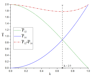
Figure 1: Bell measurement mixed with white noise: Behaviour of $\mathcal{I}_{14}^{f}$ , $\mathcal{I}_{12}^{f}$, and $\mathcal{I}_{{\rm tot}}^{f}=\mathcal{I}_{12}^{f}+\mathcal{I}_{14}^{f}$ as function of $\lambda\in\left[0,1\right]$.

Bell measurement mixed with white noise

The POVM elements are defined as

$$\mathbb{M}_{i}\left(\lambda\right) = \lambda\left|\Psi_{i}\right\rangle\left\langle\Psi_{i}\right|+\left(1-\lambda\right)\frac{\mathbb{I}}{4}$$

for $i=1,\dots,4$. The measurement is separable for $0\leq\lambda\leq\frac{1}{3}$ and entangled for $\frac{1}{3}<\lambda\leq 1$. Comparing with (13) we see that $q_{il}=\frac{1}{4}$ $\forall$ $i,l=1,\dots,4$; $x_{i}=\frac{3\lambda+1}{4}$ and $y_{ij}=\frac{1-\lambda}{4}$ $\forall$ $i,j=1,\dots,4$. Then from (14) we find that $p_{k}=\frac{1}{4}$, so all outcomes are equally probable. The post-measurement states are obtained from (15) and (18):

$$\rho_{14|k} = a\left|\Psi_{k}\right\rangle\left\langle\Psi_{k}\right|+b\sum_{j\neq k}\left|\Psi_{j}\right\rangle\left\langle\Psi_{j}\right|,$$ (27)

$$\rho_{m\,m+1|k} = c\left|\Psi_{k}\right\rangle\left\langle\Psi_{k}\right|+d\sum_{l\neq k}\left|\Psi_{l}\right\rangle\left\langle\Psi_{l}\right|,$$ (28)

for $m=1,3$, where

$$a = \frac{3\lambda+1}{4},$$

$$b = \frac{1-\lambda}{4},$$

$$c = \frac{1}{16}\left(\sqrt{3\lambda+1}+3\sqrt{1-\lambda}\right)^{2},$$

$$d = \frac{1}{16}\left(\sqrt{3\lambda+1}-\sqrt{1-\lambda}\right)^{2}.$$

Note that the states $\rho_{14|k}$ and $\rho_{14|k^{\prime}}$ are LU equivalent for $k,k^{\prime}=1,\dots,4$ and so are $\rho_{m\,m+1|k}$ and $\rho_{m\,m+1|k^{\prime}}$ for $m=1,3$ and $k,k^{\prime}=1,\dots,4$. This means that $\mathcal{I}_{14}$, $\mathcal{I}_{12}$, and $\mathcal{I}_{34}$ do not change with outcomes and the trade-off relations (22) will be the same for every outcome. In what follows, we therefore omit the subscript for measurement outcome.

From (27) and (28) and using (25) we find that

$$\mathcal{I}_{14}^{f} = 2\lambda^{2},$$

$$\mathcal{I}_{m\,m+1}^{f} = \frac{1}{2}\left(1-\lambda+\sqrt{\left(1-\lambda\right)\left(1+3\lambda\right)}\right)^{2},$$

where $m=1,3$ and $0\leq\lambda\leq 1$. Substituting the above in (22) it is easy to show that the inequalities are strict for all $0<\lambda<1$ (note that, $\lambda=1$ corresponds to the Bell measurement). So information is not conserved for $\lambda\in\left(0,1\right)$.

Let us now look at the process of information transfer as we vary $\lambda$ which controls the strength of the measurement. In Fig. 1 we have plotted the quantities $\mathcal{I}_{14}^{f}$, $\mathcal{I}_{12}^{f}$, and $\mathcal{I}_{{\rm tot}}^{f}=\mathcal{I}_{m\,m+1}^{f}+\mathcal{I}_{14}^{f}$, each of which is a function of $\lambda$.

Observations:

• At $\lambda=0$, $\rho_{14}$ is maximally mixed and $\rho_{12}$, $\rho_{34}$ are both maximally entangled. So $\mathcal{I}_{{\rm tot}}=2$.

• As $\lambda$ starts moving away from zero, we start observing information transfer throughout, even though the measurement remains separable through $\lambda\in\left[0,\frac{1}{3}\right]$.

• $\mathcal{I}_{{\rm tot}}<2$ for $\lambda\in\left(0,1\right)$ which indicates loss of information in this range. The information loss is maximum at $\lambda=\frac{2}{3}$ where $\mathcal{I}_{\text{tot}}$ attains the minimum. But note that from this point onward $\mathcal{I}_{\text{tot}}$ starts to increase, eventually reaching the maximum at $\lambda=1$ which corresponds to the Bell measurement.

• The crossover between $\mathcal{I}_{14}^{f}$ and $\mathcal{I}_{12}^{f}$ at $\lambda=\frac{2}{3}$ tells us that when the measurement is weak in the beginning, the initial pairs lose more information than that gained by $\left(1,4\right)$, but as the measurement picks up strength, this reverses, which is why the minimum is observed.

So far we have seen information is not conserved for COMs (not maximally entangled) and for measurements obtained by mixing Bell measurement with white noise. This prompted us to question whether this could be a generic feature for all measurements that are not maximally entangled. But because a general result is quite difficult to get, we explored the question within the family of Bell-diagonal measurements $\mathbb{M}\left(\lambda\right)$ and found that there exists a rank-two measurement for which this is not the case. This is discussed next.

Rank-two Bell-diagonal measurement

Here the POVM elements are defined as

$$\mathbb{M}_{1}\left(\lambda\right) = \lambda\left|\Psi_{1}\right\rangle\left\langle\Psi_{1}\right|+\left(1-\lambda\right)\left|\Psi_{2}\right\rangle\left\langle\Psi_{2}\right|,$$

$$\mathbb{M}_{2}\left(\lambda\right) = \lambda\left|\Psi_{2}\right\rangle\left\langle\Psi_{2}\right|+\left(1-\lambda\right)\left|\Psi_{1}\right\rangle\left\langle\Psi_{1}\right|,$$

$$\mathbb{M}_{3}\left(\lambda\right) = \lambda\left|\Psi_{3}\right\rangle\left\langle\Psi_{3}\right|+\left(1-\lambda\right)\left|\Psi_{4}\right\rangle\left\langle\Psi_{4}\right|,$$

$$\mathbb{M}_{4}\left(\lambda\right) = \lambda\left|\Psi_{4}\right\rangle\left\langle\Psi_{4}\right|+\left(1-\lambda\right)\left|\Psi_{3}\right\rangle\left\langle\Psi_{3}\right|,$$

for $\lambda\in\left[0,1\right]$. The measurement is entangled except at $\lambda\neq\frac{1}{2}$.

For outcome $k$, the post-measurement states are obtained from (15) and (18); in particular,

$$\rho_{14|k} = \mathbb{M}_{k}\left(\lambda\right),$$ (29)

$$\rho_{m\,m+1|k} = \sum_{l=1}^{4}\tau_{l}\left|\Psi_{l}\right\rangle\left\langle\Psi_{l}\right|,\;m=1,3,$$ (30)

where

$$\tau_{l} = \frac{1}{4}\left(1+2\sqrt{\lambda\left(1-\lambda\right)}\right),\;l=\begin{array}[]{ccc}k,k+1&\mbox{for}&k=1,3\\ k,k-1&\mbox{for}&k=2,4\end{array}$$

$$\tau_{l} = \frac{1}{4}\left(1-2\sqrt{\lambda\left(1-\lambda\right)}\right),\;\mbox{ }l\,\mbox{otherwise}.$$

Note that, $\rho_{14|k}$ is entangled $\forall\lambda$ except when $\lambda=\frac{1}{2}$ but $\rho_{12|k}$ and $\rho_{34|k}$ are separable $\forall\lambda$. Moreover, as in the previous example, the post-measurement states for different outcomes are LU equivalent and so we only need to find $\mathcal{I}_{14}^{f}$, $\mathcal{I}_{12}^{f}$, and $\mathcal{I}_{34}^{f}$ for a particular outcome.

From the expressions (29), (30) of the post-measurement states and using (25), we find that

$$\mathcal{I}_{14}^{f} = 1+\left(2\lambda-1\right)^{2},$$

$$\mathcal{I}_{m\,m+1}^{f} = 4\lambda\left(1-\lambda\right),\;m=1,3$$

for all $\lambda\in\left[0,1\right]$. Consequently,

$$\mathcal{I}_{m\,m+1}^{f}+\mathcal{I}_{14}^{f} = 2,\;m=1,3.$$

Hence, information is conserved for all $\lambda\in\left[0,1\right]$. Note however that entanglement is not conserved in any bipartition $\forall\lambda\in\left(0,1\right)$ because (a) the states $\rho_{m\,m+1}$, $m=1,3$ are separable and (b) $\rho_{14}$ is not maximally entangled whenever $\lambda\in\left(0,1\right)$.

Interestingly, information is conserved even at $\lambda=\frac{1}{2}$, i.e., when not only the measurement is separable but also all three pairs become separable. So separable measurements can conserve information even when all post-measurement states turn separable after Bob’s measurement. The functions $\mathcal{I}_{14}^{f}$, $\mathcal{I}_{12}^{f}$, and $\mathcal{I}_{{\rm tot}}^{f}$ are plotted in Fig. 2, where $\mathcal{I}_{{\rm tot}}^{f}=\mathcal{I}_{12}^{f}+\mathcal{I}_{14}^{f}$. As one can see, information gained in $\left(1,4\right)$ is always the same as information lost from the pair $\left(1,2\right)$ for all $\lambda$.

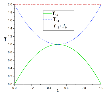
Figure 2: Rank-2 Bell-diagonal measurement: Behaviour of $\mathcal{I}_{14}^{f}$ , $\mathcal{I}_{12}^{f}$, and $\mathcal{I}_{{\rm tot}}^{f}=\mathcal{I}_{12}^{f}+\mathcal{I}_{14}^{f}$ as function of $\lambda\in\left[0,1\right]$.

V Conclusions

In this paper, we investigated information-disturbance trade-off in generalized entanglement swapping protocols. In particular, we considered protocols where starting from two Bell pairs $\left(1,2\right)$, $\left(3,4\right)$ shared between Alice and Bob, Bob and Charlie, respectively, Bob performs a two-qubit measurement on $\left(2,3\right)$ and communicates the outcome to Alice and Charlie, so that $\left(1,4\right)$ becomes correlated. We obtained trade-off inequalities between information gain in $\left(1,4\right)$ and residual information in the pairs $\left(1,2\right)$ and $\left(3,4\right)$, respectively, where information is understood as the total information contained in correlations of a two-qubit state, which is quantified in terms of an information theoretic measure of entanglement. We argued that when equality holds for any given measurement then it implies information is conserved across the bipartitions $A|BC$ and $C|BA$. We further studied these inequalities for some well-known two-qubit measurements and found the inequalities to be strict for complete orthogonal but nonmaximally entangled measurements and for Bell measurement mixed with white noise. However, rather counter-intuitively, we found that there exist rank-2 Bell-diagonal measurements that conserve information but do not conserve entanglement, and moreover, there exist separable measurements that conserve information even when all three pairs $\left(1,2\right)$, $\left(3,4\right)$, and $\left(1,4\right)$ become separable after Bob’s measurement. This is particularly interesting because it shows that correlations in an entangled pair can be distributed in separable pairs in nontrivial ways so that there is no loss of information.

Our results open up some interesting avenues for further research. Let us begin by noting that the inequalities (1) are basic in nature as they hold for all entanglement swapping protocols. On the other hand, the second set of inequalities given by (2), and the subsequent interpretation of conservation/loss of information, crucially depends on the fact that the initial states are maximally entangled. So it would be very interesting to obtain inequalities similar to that of (2) for arbitrary initial states. This might, however, require considering a different information measure, which should ideally be a LOCC monotone.

Finally, we would like to remark that it is important to explore and understand the basic questions related to information transfer in entanglement swapping-like protocols, and we hope our results would stimulate further research on this topic.

Acknowledgement.

S.B. is supported in part by SERB (Science and Engineering Research Board), Department of Science and Technology, Government of India through Project No. EMR/2015/002373.

References

• (1) M. Zukowski, A. Zeilinger, M. A. Horne, and A. K. Ekert, “Event-ready-detectors” Bell experiment via entanglement swapping, Phys. Rev. Lett. 71, 4287 (1993).
• (2) S. Bose, V. Vedral, and P. L. Knight, Multiparticle generalization of entanglement swapping, Phys. Rev.A 57, 822 (1998).
• (3) G. Gour and Barry C. Sanders, Remote preparation and distribution of bipartite entangled states, Phys. Rev. Lett. 93, 260501 (2004).
• (4) S. Perseguers, C. I. Cirac, A. Acin, M. Lewenstein, and J. Wehr, Entanglement distribution in pure-state quantum networks, Phys. Rev.A 77, 022308 (2008).
• (5) S. Perseguers, G. J. Lapeyre Jr, D. Cavalcanti, M. Lewenstein, and A. Acin, Distribution of entanglement in large-scale quantum networks, Rep. Prog. Phys. 76, 096001 (2013).
• (6) A. Wojcik, J. Modlawska, A. Grudka and M. Czechlewski, Violation of Clauser-Horne-Shimony-Holt inequality for states resulting from entanglement swapping, Phys. Lett. A 374, 48, 4831 (2010).
• (7) W. Klobus, W. Laskowski, M. Markiewicz, and A. Grudka, Nonlocality activation in entanglement-swapping chains, Phys. Rev. A 86, 020302(R) (2012).
• (8) A. Zeilinger, A foundational principle for quantum mechanics, Foundations of Physics 29, 631-643 (1999).
• (9) C. Brukner and A. Zeilinger, Operationally Invariant Information in Quantum Measurements, Phys. Rev. Lett. 83, 3354 (1999).
• (10) C. Brukner, M. Zukowski, and A. Zeilinger, The essence of entanglement, quant-ph/0106119.
• (11) C. Brukner, M. Aspelmeyer, and A. Zeilinger, Complementarity and information in delayed-choice for entanglement swapping, Foundations of Physics 35, 11 (2005).
• (12) S. Camalet, Measure-independent anomaly of nonlocality,Phys. Rev. A 96, 052332 (2017).
• (13) That $\mathcal{I}$ is a not a LOCC monotone can be understood as follows. Recall that, for any two-qubit state, $\mathcal{I}\left(\rho\right)=\frac{B\left(\rho\right)^{2}}{4}$, where $\mathcal{B}\left(\rho\right)$ is the maximal mean value of the Bell-CHSH observable. Recently, it has been proven that any Bell local $\rho$ with hidden nonlocality can be deterministically transformed into a nonlocal state using LOCC (Camlet-2017, ). So $\mathcal{B}\left(\rho\right)$ is not a LOCC monotone and therefore neither is $\mathcal{I}\left(\rho\right)$.
• (14) B. Toner and F. Verstraete, Monogamy of Bell correlations and Tsirelson’s bound, arXiv:quant-ph/0611001.
• (15) S. Cheng and M. J. W. Hall, Anisotropic invariance and the distribution of quantum correlations, Phys. Rev. Lett. 118, 010401 (2017).
• (16) R. Horodecki, P. Horodecki, and M. Horodecki, Violating Bell inequality by mixed spin-1/2 states: necessary and sufficient condition, Phys.Lett.A 200,340 (1995).
• (17) R. Horodecki, Two spin-1/2 mixture and Bell inequalities, Phys.Lett.A 210,223 (1996).