A Primitive Variable Discrete Exterior Calculus Discretization of Incompressible Navier-Stokes Equations over Surface Simplicial Meshes

Abstract

A conservative primitive variable discrete exterior calculus (DEC) discretization of the Navier-Stokes equations is performed. An existing DEC method (Mohamed, M. S., Hirani, A. N., Samtaney, R. (2016). Discrete exterior calculus discretization of incompressible Navier-Stokes equations over surface simplicial meshes. Journal of Computational Physics, 312, 175-191) is modified to this end, and is extended to include the energy-preserving time integration and the Coriolis force to enhance its applicability to investigate the late time behavior of flows on rotating surfaces, i.e., that of the planetary flows. The simulation experiments show second order accuracy of the scheme for the structured-triangular meshes, and first order accuracy for the otherwise unstructured meshes. The method exhibits second order kinetic energy relative error convergence rate with mesh size for inviscid flows. The test case of flow on a rotating sphere demonstrates that the method preserves the stationary state, and conserves the inviscid invariants over an extended period of time.

1 Introduction

Recently, structure preserving numerical methods that satisfy the mathematical and physical properties of the governing equations are increasingly becoming popular [1, 2, 3]. One of such methods is discrete exterior calculus (DEC). It uses integral quantities / discrete forms as the primary unknowns and transforms the continuous partial differential equation (PDE) system into a discrete algebraic system such that all errors/approximations occur only at the algebraic level and not in the approximation of the differential operators of the PDE [4]. Thus, DEC is known to preserve some of the underlying physical and mathematical properties of the continuous PDE system.

DEC is the discrete counterpart of smooth exterior calculus, which is more natural tool than tensor calculus in numerous situations. The theory of exterior calculus and differential forms dates back to the pioneering work of Poincaré [5] (who presented the notion of line and surface integrals), Cartan [6] ( who formalized the notion of differential forms), and Goursat [7] ( who noted that the three theorems of vector calculus, viz. Gauss, Green, and Stokes are all special cases of a generalized Stokes theorem for differential forms). Subsequently, there were further theoretical developments (for example, see [8, 9, 10]). However, there were limited applications of this theory to solve physical problems, until the theory of discrete exterior calculus was developed (see [11, 12, 13] and the references therein). As this theory advanced, DEC made its way to the applications such as computer graphics and computer vision [14, 15, 16, 13, 17, 18, 19] to mitigate the effects of numerical viscosity that causes detrimental visual consequences, and fluid flows [20, 21, 22, 23] to preserve the physical properties of the governing equations, i.e, to conserve secondary quantities, such as kinetic energy and/or discretely preserving Kelvin’s circulation theorem. Developing such physically conservative discretizations, for Navier-Stokes equations for example, is favorable for many physical applications such as turbulent flows [24] and shallow-water simulations [25] to avoid undesirable numerical artifacts.

Apart from DEC, some staggered mesh methods have also demonstrated conservation of secondary (kinetic energy and vorticity) physical quantities in addition to the primary ones (mass and momentum) [26]. Nicolaides [27] and Hall et al. [28] developed staggered mesh methods, also known as covolume methods, for unstructured meshes. The covolume discretization commences by taking dot product of the momentum equation with the unit normal to each face of the triangular / tetrahedral elements, reducing the velocity vector to a scalar flux (equal to the mass flux across the face for an incompressible flow with constant density) defined on each face; and the pressure is defined at the circumcenter of each triangular / tetrahedral element. Nicolaides [29] estimated the accuracy of the covolume method to be second order for a mesh with all its triangular elements having the same circumradii (i.e., structured-triangular mesh), and to be first order otherwise. Perot [30] demonstrated the conservation properties of the covolume method. The divergence form of the Navier-Stokes equations conserved the momentum and kinetic energy both locally and globally, and the rotational form conserved the circulation and kinetic energy locally and globally for both 2D [30] and 3D [24] discretizations. A main advantage of DEC discretizations is their applicability to simulate flows over curved surfaces, unlike the covolume approach [21]. Due to its intrinsic coordinate independent nature, DEC based implementations work on both planar domains and curved surfaces without any change. Its independence of the embedding space dimension as well as the details of the embedding characterizes a key difference between DEC and the covolume method. In the latter, face normal vectors, with which dot product of the momentum equation is performed for the discretization, may not be unique for a simplicial mesh approximation of a curved surface.

Here, we extend an existing stream function formulation DEC scheme [21], to the primitive variable formulation. To compute the aerodynamic forces for the flows past bluff / streamlined bodies, the stream function formulation requires a posteriori computation of the pressure field from the stream function field, which may introduce some error. The primitive variable formulation computes the pressure field as a part of the DEC solution and is more relevant for such physical applications. Moreover, the method is extended to include the Coriolis force, in order to enhance its applicability to vortical flows on rotating surfaces which are usually used to model planetary flows. In addition, an energy-preserving time integrator [17] is incorporated, to enhance applicability of the method to study the late time behavior of such (vortical flows on rotating surfaces) initial value problems.

2 Primitive Variable DEC Formulation

A primitive variable DEC formulation is presented here, extending an existing stream function method [21]. First, the Navier-Stokes equations are expressed in exterior calculus notation, and then the DEC discretization is derived. The resultant degrees of freedom are the primitive variables, namely the velocity 1-form and the pressure 0-form. We recommend for readers unfamiliar with DEC to read through the appendix for a primer on discrete exterior calculus before reading through this section.

2.1 Exterior Calculus Expression of the Navier-Stokes Equations

For an incompressible flow of a homogeneous fluid with unit density, on a compact smooth Riemannian surface, the vector calculus notation of Navier-Stokes equations in a rotating frame of reference are as follows.

$$\frac{\partial\mathbf{v}}{\partial t}-\mu\left[-\Delta^{dR}\mathbf{v}+2\kappa\mathbf{v}\right]+\nabla_{\mathbf{v}}\mathbf{v}+\textrm{grad}_{S}p+f\hat{k}\times\mathbf{v}=0,$$ (1)

$$\textrm{div}_{S}\mathbf{v}=0,$$ (2)

where $\mathbf{v}$ is the tangential surface velocity, $p$ is the effective surface pressure (which includes the centrifugal force), $\mu$ is the dynamic viscosity, $\Delta^{dR}$ is the surface Laplace-DeRham operator, $\kappa$ is the surface Gaussian curvature, $\nabla_{\mathbf{v}}$ is the covariant directional derivative, $\textrm{grad}_{S}$ is the surface gradient, $\textrm{div}_{S}$ is the surface divergence, $f$ is the Coriolis parameter, and $\hat{k}$ is the unit vector in the direction of the axis of rotation. The Laplace-DeRham operator and the Gaussian curvature term are a result of the divergence of the deformation tensor and the non-commutativity of the second covariant derivative in curved spaces [22]. Following Mohamed et al. [21], with the additional curvature term $-2\mu\kappa u$ and Coriolis force $f\hat{k}\times\mathbf{v}$, the 2D coordinate invariant form of equations (1) - (2), for constant $\kappa$ (for convenience, its variation is addressed later in Sec. 2.2.2), read

$$\frac{\partial u}{\partial t}-\mu\ast\textrm{d}\ast\textrm{d}u-2\mu\kappa u+\ast\left(u\wedge\ast\textrm{d}u\right)+\textrm{d}p^{d}+\ast\left(u\wedge\ast f_{dual2}\right)=0.$$ (3)

$$\ast\textrm{d}\ast u=0.$$ (4)

Here, $u$ is the 1-form velocity, d is the exterior derivative, $\ast$ is the Hodge star operator, $\wedge$ is the wedge product operator, $p^{d}=p+\frac{1}{2}\left(u\left(\mathbf{v}\right)\right)$ is the effective dynamic pressure 0-form, $N$ is the space dimension, and the Coriolis force $f\hat{k}\times\mathbf{v}=\ast\left(u\wedge\ast f_{dual2}\right)$ [31], where $f_{dual2}$ is the dual 2-form corresponding to $f$. Equations (3) - (4) correspond to smooth exterior calculus expressions, and are still continuous.

2.2 Discrete Exterior Calculus Expression

The discretization consists of the domain discretization, and discretization of the governing equations, i.e., discrete exterior calculus expression of the governing equations (equations (3) and (4)).

2.2.1 Domain discretization

Two-dimensional (2D) domain discretization is considered assuming a primal simplicial mesh. The objects of this simplicial mesh are the triangles (primal 2-simplices), edges of the triangles (primal 1-simplices), and the vertices / nodes (primal 0-simplices). A circumcentric dual mesh is considered, which consists of dual polygons, the edges of the dual polygons, and the dual vertices / nodes. The dual to a primal triangle is its circumcenter (which is a dual node), that to a primal edge is the perpendicular dual edge connecting the circumcenters of the two triangles sharing this primal edge, and that to a primal node is the polygon formed by the edges dual to the primal edges connected to this node. For a triangular mesh representing a curved surface, the dual edges are kinked lines and the dual cells are non-planar. Counterclockwise orientation of both the primal mesh (triangles/primal 2-simplices) and dual mesh (polygons) is assumed to be positive. The choice of the orientation of the primal edges (primal 1-simplices) is arbitrary, however it induces the dual edges orientations. The orientation of the dual edges is derived simply by rotating the primal edge orientation 90 degrees along the triangles orientation (i.e., counterclockwise). Moreover, there is no requirement such as the triangles need to be Delaunay [32].

2.2.2 Discrete exterior calculus expression of the governing equations

First we need to specify the correspondence between the discrete variables (the forms) and the mesh objects (vertices, edges etc.). This requires that we define the discrete forms, or discretize the smooth forms. We then determine the discrete operators and substitute the smooth exterior calculus operators with their discrete counterparts. For the current discretization, we define the velocity 1-form $u$ in all terms (except one in the nonlinear term which will be discussed later) on dual edges in equation (3), i.e., we chose the velocity 1-form $u$ to be a dual 1-form. The dual 1-form represents the velocity integration along the dual edges and hence corresponds to the mass flux across the primal edges. With this choice, for consistency, each term (time derivative, convection, diffusion, pressure gradient) in equation (3) must be a dual 1-form. This choice of the velocity 1-form requires the dynamic pressure 0-form $p^{d}$ to be defined at the dual nodes or the triangles circumcenters (to be defined as a dual 0-form), so that the pressure gradient term $\textrm{d}p^{d}$ is a dual 1-form, consistent with the choice of $u$ as the dual 1-form. For consistency, since the convective term $\ast\left(u\wedge\ast\textrm{d}u\right)$ is a dual 1-form, the wedge product term $\left(u\wedge\ast\textrm{d}u\right)$ is a primal 1-form (defined on primal edges). Since $u$ is a 1-form, and hence $\ast\textrm{d}u$ is a 0-form (in 2D), and therefore the operands of the wedge product are a 1-form and a 0-form, such that the resultant (primal 1-form) must be defined on primal edges. This requires that both wedge product operands are defined on primal mesh objects. Accordingly, the velocity 1-form in the first operand $\left(u\right)$ of the wedge product term is defined on the primal edges, whereas the velocity 1-form in the second operand $\left(\ast\textrm{d}u\right)$ is defined on the dual edges, so that the 0-form $\ast\textrm{d}u$ is defined on the primal nodes. Following Mohamed et al. [21], the definitions and expressions for the discrete d, $\ast$, and $\wedge$ operators, the DEC discretization of equation (3) now reads (in 2D)

$$\frac{U^{n+1}-U^{n}}{\triangle t}-\mu\ast_{1}\textrm{d}_{0}\ast_{0}^{-1}\left[\left[-\textrm{d}_{0}^{T}\right]U+\textrm{d}_{b}V\right]-2\mu\kappa U$$

$$+\ast_{1}W_{V}\ast_{0}^{-1}\left[\left[-\textrm{d}_{0}^{T}\right]U+\textrm{d}_{b}V\right]+\textrm{d}_{1}^{T}P^{d}+\ast_{1}W_{V}\ast_{0}^{-1}f_{dual2}=0.$$ (5)

Here, $U$ is the vector containing the discrete dual velocity 1-forms for all mesh dual edges, $V$ is the vector containing the discrete primal velocity 1-forms for all mesh primal edges, and $P^{d}$ is the vector containing discrete effective dynamic pressure 0-forms for all mesh dual vertices, $\Delta t$ is the discrete time interval between the current time instant $n+1$ and the previous time instant $n$. Note that the time-centering of all terms except the one involving the time derivative is discussed later in sections 2.2.3 and 2.2.4. The matrix $W_{V}$ is defined as $W_{V}=0.5diag(V)\left|\textrm{d}_{0}\right|$ and is a sparse $N_{1}\times N_{0}$ matrix, where $N_{1}$ is the number of primal edges and $N_{0}$ is the number of primal nodes. Moreover, the term $\ast_{0}^{-1}\left[-\textrm{d}_{0}^{T}\right]U$ represents vorticity and is a vector with $N_{0}$ entries. The term $W_{V}\ast_{0}^{-1}\left[-\textrm{d}_{0}^{T}\right]U$ is equivalent to taking the average, at each primal edge, of the vorticity $\ast_{0}^{-1}\left[-\textrm{d}_{0}^{T}\right]U$ evaluated at the edge’s nodes and multiply it by the edge’s tangential velocity 1-form $v$. Thus, this term evaluates the first wedge product. Moreover, since $\ast f_{dual2}$ is a primal 0-form, the 1-form velocity $u$ in the second wedge product also has to be the primal 1-form for consistency. Thus the term $\ast_{1}W_{V}\ast_{0}^{-1}f_{dual2}$ evaluates the second wedge product. The tangential velocity 1-form $v$ at each primal edge is evaluated following Mohamed et al. [21].

The boundary of the dual 2-cells to the primal nodes on the domain boundary includes primal boundary edges. Since $\left[-\textrm{d}_{0}^{T}\right]$ matrix is the boundary operator of these dual 2-cells, it is complemented by an additional operator $\textrm{d}_{b}$ to account for the primal boundary edges. The operation $\left[-\textrm{d}_{0}^{T}\right]U$ evaluates the circulation of the velocity 1-forms $u$ along the dual 2-cells boundaries. The operation $\textrm{d}_{b}V$ complements this circulation for the dual 2-cells part of whose boundaries consists of primal edges. The matrix $\textrm{d}_{b}=0.5\left|\textrm{d}_{0}^{T}\right|\textrm{diag}\left(\textrm{d}_{1}^{T}\mathds{1}\right)$ , where $\left|\textrm{d}_{0}^{T}\right|$ is the matrix $\textrm{d}_{0}^{T}$ with all entries made positive and $\mathds{1}$ is a vector of ones with $N_{2}$ (number of primal 2-simplices / triangles) entries, and $\textrm{diag}\left(\cdot\right)$ is a diagonal matrix consisting of the enclosed vector entries.

Since the mass flux primal 1-form (the mass flux across the primal edge) is defined as the integral of the normal velocity (normal to the primal edge) along the primal edge, the vector containing mass flux primal 1-form $u^{\ast}$ for all mesh primal edges can be expressed as $U^{*}=-\ast_{1}^{-1}U$ or $U=\ast_{1}U^{*}$. After this substitution, Eq. (5) reads

$$\ast_{1}\left[\frac{\left(U^{*}\right)^{n+1}-\left(U^{*}\right)^{n}}{\triangle t}\right]-\mu\ast_{1}\textrm{d}_{0}\ast_{0}^{-1}\left[\left[-\textrm{d}_{0}^{T}\right]\ast_{1}U^{*}+\textrm{d}_{b}V\right]-2\mu\kappa\ast_{1}U^{\ast}$$

$$+\ast_{1}W_{V}\ast_{0}^{-1}\left[\left[-\textrm{d}_{0}^{T}\right]\ast_{1}U^{*}+\textrm{d}_{b}V\right]+\textrm{d}_{1}^{T}P^{d}+\ast_{1}W_{V}\ast_{0}^{-1}f_{dual2}=0.$$ (6)

Applying the Hodge star $\ast_{1}^{-1}$ to equation (6), and considering the property $\ast_{1}^{-1}\ast_{1}=-1$, we have

$$-\frac{\left(U^{*}\right)^{n+1}-\left(U^{*}\right)^{n}}{\triangle t}+\mu\textrm{d}_{0}\ast_{0}^{-1}\left[\left[-\textrm{d}_{0}^{T}\right]\ast_{1}U^{*}+\textrm{d}_{b}V\right]+2\mu\kappa U^{*}$$

$$-W_{V}\ast_{0}^{-1}\left[\left[-\textrm{d}_{0}^{T}\right]\ast_{1}U^{*}+\textrm{d}_{b}V\right]+\ast_{1}^{-1}\textrm{d}_{1}^{T}P^{d}-W_{V}\ast_{0}^{-1}f_{dual2}=0.$$ (7)

In general, $\kappa$ may not be uniform. For domains with non-uniform $\kappa$, it may be treated as a primal 0-form (defined at the primal vertices). Now the curvature term $\left(2\mu\kappa U^{\ast}\right)$ is modified and Eq. (7) reads

$$-\frac{\left(U^{*}\right)^{n+1}-\left(U^{*}\right)^{n}}{\triangle t}+\mu\textrm{d}_{0}\ast_{0}^{-1}\left[\left[-\textrm{d}_{0}^{T}\right]\ast_{1}U^{*}+\textrm{d}_{b}V\right]+2\mu KU^{*}$$

$$-W_{V}\ast_{0}^{-1}\left[\left[-\textrm{d}_{0}^{T}\right]\ast_{1}U^{*}+\textrm{d}_{b}V\right]+\ast_{1}^{-1}\textrm{d}_{1}^{T}P^{d}-W_{V}\ast_{0}^{-1}f_{dual2}=0.$$ (8)

Here, $K$ is half times a matrix containing values of $\kappa$ at the nodes of each edge, and it accounts for the wedge product of the primal zero form $\kappa$ with the primal 1-form $u^{\ast}$. With reference to temporal discretization, we first implemented the Euler first order time integration scheme. Later, in order to enhance the ability to study the late-time behavior of initial value problems, we implemented the energy-preserving time integration [17]. Both time integration schemes are discussed below.

2.2.3 Euler first order time integration

We treat the viscous, curvature and pressure gradient terms implicitly, and the convection and Coriolis force terms explicitly. In order to obtain a linear representation for the convective term, we evaluate the tangential velocity 1-forms $V$ through an interpolation of previously-known normal velocity 1-forms $U$. Therefore, we have

$$-\frac{\left(U^{*}\right)^{n+1}-\left(U^{*}\right)^{n}}{\triangle t}+\mu\textrm{d}_{0}\ast_{0}^{-1}\left[\left[-\textrm{d}_{0}^{T}\right]\ast_{1}\left(U^{*}\right)^{n+1}+\textrm{d}_{b}\left(V\right)^{n}\right]+2\mu K\left(U^{\ast}\right)^{n+1}$$

$$-\left(W_{V}\right)^{n}\ast_{0}^{-1}\left[\left[-\textrm{d}_{0}^{T}\right]\ast_{1}\left(U^{*}\right)^{n}+\textrm{d}_{b}\left(V\right)^{n}\right]+\ast_{1}^{-1}\textrm{d}_{1}^{T}\left(P^{d}\right)^{n+1}$$

$$-\left(W_{V}\right)^{n}\ast_{0}^{-1}f_{dual2}=0,$$ (9)

or

$$\left[-\frac{1}{\triangle t}I+\mu\textrm{d}_{0}\ast_{0}^{-1}\left[-\textrm{d}_{0}^{T}\right]\ast_{1}+2\mu K\right]\left(U^{*}\right)^{n+1}+\ast_{1}^{-1}\textrm{d}_{1}^{T}\left(P^{d}\right)^{n+1}=F,$$ (10)

where $I$ is an identity matrix, and

$$F=-\frac{1}{\triangle t}\left(U^{*}\right)^{n}-\mu\textrm{d}_{0}\ast_{0}^{-1}\textrm{d}_{b}\left(V\right)^{n}$$

$$+\left(W_{V}\right)^{n}\ast_{0}^{-1}\left[\left[-\textrm{d}_{0}^{T}\right]\ast_{1}\left(U^{*}\right)^{n}+\textrm{d}_{b}\left(V\right)^{n}+f_{dual2}\right].$$ (11)

The continuity equation is expressed as

$$\left[\textrm{d}_{1}\right]\left(U^{*}\right)^{n+1}+\left[0\right]\left(P^{d}\right)^{n+1}=0.$$ (12)

Equations (10) - (12) represent a set of linear equations with $U^{\ast}$ and $P^{d}$ as the solution vectors, which is solved along with usual boundary conditions depending on the considered test case.

2.2.4 Energy-preserving time integration

The midpoint integration is assumed for the update in time of the advection, diffusion, curvature, pressure gradient and Coriolis force terms [17], i.e., these terms are evaluated at time $n+\frac{1}{2}$. Thus we have,

$$-\frac{\left(U^{*}\right)^{n+1}-\left(U^{*}\right)^{n}}{\triangle t}+\frac{1}{2}\left[\mu\textrm{d}_{0}\ast_{0}^{-1}\left(\left[-\textrm{d}_{0}^{T}\right]\ast_{1}\left(U^{*}\right)^{n+1}+\textrm{d}_{b}\left(V\right)^{n+1}\right)\right.$$

$$\left.+\mu\textrm{d}_{0}\ast_{0}^{-1}\left(\left[-\textrm{d}_{0}^{T}\right]\ast_{1}\left(U^{*}\right)^{n}+\textrm{d}_{b}\left(V\right)^{n}\right)\right]+\frac{1}{2}\left[2\mu K\left(U^{\ast}\right)^{n+1}+2\mu K\left(U^{\ast}\right)^{n}\right]$$

$$-\frac{1}{2}\left[\left(W_{V}\right)^{n+1}\ast_{0}^{-1}\left(\left[-\textrm{d}_{0}^{T}\right]\ast_{1}\left(U^{*}\right)^{n+1}+\textrm{d}_{b}\left(V\right)^{n+1}\right)\right.$$

$$\left.+\left(W_{V}\right)^{n}\ast_{0}^{-1}\left(\left[-\textrm{d}_{0}^{T}\right]\ast_{1}\left(U^{*}\right)^{n}+\textrm{d}_{b}\left(V\right)^{n}\right)\right]+\ast_{1}^{-1}\textrm{d}_{1}^{T}\left(P^{d}\right)^{n+\frac{1}{2}}$$

$$-\frac{1}{2}\left[\left(W_{V}\right)^{n+1}\ast_{0}^{-1}f_{dual2}+\left(W_{V}\right)^{n}\ast_{0}^{-1}f_{dual2}\right]=0.$$ (13)

Rearranging the terms, we have

$$\left[-\frac{1}{\Delta t}I+\mu K+\frac{1}{2}\mu\textrm{d}_{0}\ast_{0}^{-1}\left[-\textrm{d}_{0}^{T}\right]\ast_{1}-\frac{1}{2}\left(W_{V}\right)^{n+1}\ast_{0}^{-1}\left[-\textrm{d}_{0}^{T}\right]\ast_{1}\right]\left(U^{*}\right)^{n+1}$$

$$+\ast_{1}^{-1}\textrm{d}_{1}^{T}\left(P^{d}\right)^{n+\frac{1}{2}}=F,$$ (14)

with

$$F=-\frac{1}{\Delta t}\left(U^{*}\right)^{n}-\mu K\left(U^{*}\right)^{n}-\frac{1}{2}\mu\textrm{d}_{0}\ast_{0}^{-1}\left(\left[-\textrm{d}_{0}^{T}\right]\ast_{1}\left(U^{*}\right)^{n}+\textrm{d}_{b}\left(V\right)^{n}\right.$$

$$\left.+\textrm{d}_{b}\left(V\right)^{n+1}\right)+\frac{1}{2}\left(W_{V}\right)^{n+1}\ast_{0}^{-1}\textrm{d}_{b}\left(V\right)^{n+1}$$

$$+\frac{1}{2}\left(W_{V}\right)^{n}\ast_{0}^{-1}\left(\left[-\textrm{d}_{0}^{T}\right]\ast_{1}\left(U^{*}\right)^{n}+\textrm{d}_{b}\left(V\right)^{n}\right)$$

$$+\frac{1}{2}\left[\left(W_{V}\right)^{n+1}+\left(W_{V}\right)^{n}\right]\ast_{0}^{-1}f_{dual2}.$$ (15)

Equation (14) along with equation (12), and the relevant boundary conditions (depending on the test case) form a non-linear system of equations. These are solved using Picard’s iterative method, with previous time-step value used as an initial guess for each time-step and a convergence criterion of $L_{2}$ norm on the residual of $\left\|R\right\|_{2}\leq 10^{-8}$. It is worth noting that the current discretization is different from that in [17] for the convective term spatial discretization and the inclusion of both surface curvature effect and Coriolis force.

3 Results and Discussions

In order to assess the accuracy of the scheme, several test cases are performed. All test cases of flow past a cylinder are solved using the Euler time integration scheme. The energy-preserving time integration scheme is then employed for the remaining test cases.

3.1 Flow Past a Stationary Circular Cylinder

The computational domain consists of a rectangular plane with a circular cylinder embedded on it. The circular cylinder contour embedded on the surface is generated by intersecting a cylinder of diameter D = 1 with the surface. The domain lengths upstream and downstream of the cylinder are 10D and 60D, respectively, and the domain width on either side of the cylinder is 10D. These domain sizes are usual in computational investigations of flow past a cylinder. Uniform normal velocity of unity is assumed at the inlet. Outflow boundary condition is assumed at the outlet. Free-slip boundary condition is considered on the top and bottom boundaries, whereas no-slip boundary condition is assumed on the cylinder wall. The computational domain is discretized using a triangular mesh (consisting of approximately 160k elements) with locally refined mesh in the vicinity of the cylinder and in the wake. Reynolds numbers ($Re=\rho u_{\infty}D/\mu$) = 40, 100, and 1000 are considered. Here, $\rho$ and $u_{\infty}$ are the fluid density (taken to be unity) and the free stream velocity at the inlet, respectively.

The flow exerts pressure and viscous forces on the cylinder, and the net force acting on the cylinder is expressed as [33]

$$\vec{F}=\int_{S}-p\vec{n}dA+\mu\int_{S}\vec{\omega}\times\vec{n}dA,$$ (16)

where $p$ is the static pressure, $\vec{n}$ is the unit normal facing outward of the cylinder, and $\vec{\omega}$ is the vorticity vector (normal to the embedding surface). The integration is carried out over the total surface area $S$ (perimeter here) of the cylinder. The discrete expression of the force vector reads

$$\vec{F}=\sum_{k=1}^{N}-p_{k}\vec{n}_{k}l_{k}+\mu\sum_{k=1}^{N}l_{k}\vec{\omega}_{k}\times\vec{n}_{k},$$ (17)

where the summation is over the cylinder $N$ boundary edges. Here, global $(x,y)$ coordinate system is considered with the cylinder axis intersection with the embedding surface as the origin. The $x$ and $y$ coordinates are along the streamwise and cross-streamwise directions, respectively. The static pressure $p_{k}$ is in the triangles adjacent to the boundary edges, $\vec{n}_{k}$ is the unit vector normal to the edge, and $l_{k}$ is the edge length. The vorticity vector is $\vec{\omega}_{k}=\vec{n}_{k,s}|\omega_{k}|$, where $\vec{n}_{k,s}$ is the unit normal to the embedding surface at the boundary edge midpoint. The vorticity magnitude $|\omega_{k}|$ is calculated by averaging the known vorticity on both of the edge nodes. The drag force $F_{d}$ and the lift force $F_{l}$ are respectively the streamwise and cross-streamwise components of the force vector $\vec{F}$, i.e., are the $x$ and $y$ components of the force vector $\vec{F}$. We calculate the drag coefficient, lift coefficient, and Strouhal number as $C_{d}=F_{d}/\left(\frac{1}{2}\rho u_{\infty}^{2}D\right)$, $C_{l}=F_{l}/\left(\frac{1}{2}\rho u_{\infty}^{2}D\right)$, and $St=fD/u_{\infty}$, respectively. Here, $\rho$ is the fluid density (taken to be unity), $u_{\infty}$ is the flow velocity at the inlet boundary of the domain (also taken to be unity), and $f$ is the vortex shedding frequency.

Table 1 reports the drag coefficient mean values. The computed values are $1.605$, $1.386$, and $1.544$ at $Re=40,100$, and $1000$, respectively. They agree well with that reported in the literature (e.g., at $Re=40$: $1.6$ [34], $1.618$ [35]; at $Re=100$: $1.38$ [34], $1.37$ [36]; at $Re=1000$: $1.5144$ [37], $1.5$ [38]). Table 1 also reports the RMS values of the lift coefficient. We compute the values to be $0.248$, and $1.081$ at $Re=100$, and $1000$, respectively. They are within the range of values reported in the literature (e.g., at $Re=100$: $0.233$ [39]; at $Re=1000$: $1.0494$ [37]). In passing, it is worth noting that the predicted values of the mean drag coefficient and RMS lift coefficient using the stream function formulation [21] are $1.337$ and $0.171$, respectively at $Re=100$. The drag coefficient is predicted correctly, but the lift coefficient is under-predicted. The under-prediction of the lift coefficient may be, as already discussed before (see section 1), because of the error induced in posterior computation of the pressure field. Table 1 reports the Strouhal number values. The Strouhal number is computed as $0.171$, and $0.239$ at $Re=100$, and $1000$, respectively, which is within the range of values reported in the literature (e.g., at $Re=100$: $0.172$ [34], $0.166$ [39]; at $Re=1000$: $0.237$ [37], $0.244$ [40]).

Reference	$Re=40$	$Re=100$			$Re=1000$
	$C_{d}$	$C_{d}$	$C_{l}$	$St$	$C_{d}$	$C_{l}$	$St$
		(mean)	(RMS)		(mean)	(RMS)
Present study	1.605	1.386	0.248	0.171	1.544	1.081	0.239
Russell and Wang [34]	1.600	1.380	-	0.172	-	-	-
Le et al. [36]	1.560	1.370	-	0.160	-	-	-
Stålberg et al. [39]	1.53	1.32	0.233	0.166	-	-	-
Kawaguti [35]	1.618	-	-	-	-	-	-
Dennis and Chang [41]	1.522	-	-	-	-	-	-
Henderson and Karniadakis [37]	-	-	-	-	1.5144	1.0494	0.237
Sheard et al. [38]	-	-	-	-	1.500	-	-
Rajani et al. [40]	-	1.342	-	0.166	1.492	-	0.244

Table 1: Mean drag coefficient, RMS lift coefficient, and Strouhal number for flow past a stationary circular cylinder case.

Figure 1 shows the plots of time averaged pressure coefficient $C_{p}=\left(p-p_{\infty}\right)/\\ \left(\frac{1}{2}\rho u_{\infty}^{2}\right)$ as a function of the angular position on the cylinder surface ($\theta$) at $Re=100$. Here, $p_{\infty}$ is the free stream pressure. The current results agree well with literature.

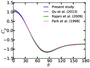
Figure 1: Pressure coefficient as a function of angular position on the cylinder for flow past a stationary circular cylinder case.

The instantaneous flow separation angle values $\left(\theta_{sep}\right)$ are summarized in table 2. They are determined to be $54.75^{\circ}$, $116.55$, $108.87$ at $Re=40$, $100$ and $1000$, respectively. They are within the range mentioned in the literature (e.g., [42], [43], [40]).

Reference	$Re=40$ (from	$Re=100$ (from	$Re=1000$ (from
	downstream	upstream	upstream
	stagnation point)	stagnation point)	stagnation point)
Present study	54.75	116.55	108.87
Kawaguti and Jain [42]	53.7	-	-
Taneda [43]	53.0	-	-
Rajani et al. [40]	-	117.05 $\pm$ 2.83	100.17 $\pm$ 18.9
		(periodic variation)	(periodic variation)

Table 2: Values of flow separation angle (in degrees) for flow past a stationary circular cylinder case.

There is an attached stationary pair of vortices in the cylinder wake at $Re=40$, the length of which is defined as the distance between the cylinder center and the end of the stationary vortex. The vortex pair length is determined to be $2.78$, which is within the range reported in the literature (e.g., $3.01$ [42], and $2.64$ [44]).

3.2 Flow Past a Rotating Circular Cylinder

The same flow configuration as described in section in 3.1 is used, except that the cylinder now has a non-zero tangential velocity. Reynolds number of $200$ is considered. Non-dimensional tangential velocities $\alpha=\left(D/2\right)\omega/u_{\infty}=2.5$ and $\alpha=3.0$ are employed. Here, $\omega$ is the tangential velocity of the cylinder. Since the cylinder is rotating, there is non-zero lift force acting on the cylinder. The lift coefficient $\left(C_{L}\right)$ (as already defined in section 3.1) values are reported in table 3. For $\alpha=2.5$ and $3$, the values of $C_{L}$ are found to be $-7.641$ and $-10.413$, respectively, which agree with the values $-7.63$ and $-10.329$ reported in [45].

Reference	$\alpha$	$C_{L}$
Present study	$2.5$	$-7.641$
	$3.0$	$-10.413$
Mittal and Kumar [45]	$2.5$	$-7.63$
	$3.0$	$-10.329$

Table 3: Lift coefficient for the flow past a rotating circular cylinder case

Figure 2 shows the plots of pressure coefficient as a function of the angular position on the cylinder surface ($\theta$) for $\alpha=2.5$ and $3.0$ at $Re=200$. They agree with that reported in [45].

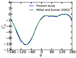
(a)

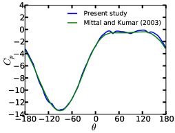
(b)

Figure 2: Pressure coefficient as a function of angular position on the cylinder for the flow past a rotating cylinder case. (a) $\alpha=2.5$, (b) $\alpha=3.0$.

3.3 Flow Past a Stationary Circular Cylinder on a Locally Curved Surface

The same flow configuration as the one described in section 3.1 is employed except that now there is a bump present in the cylinder wake. The bump is described by

$$z=h\exp\left(-\left(\left(x-x_{0}\right)^{2}+\left(y-y_{0}\right)^{2}\right)/\left(2r_{0}^{2}\right)\right)$$ (18)

where the parameters describing the bump location read: $x_{0}=6.0,y_{0}=0.5,h=1.6,1/\left(2r_{0}^{2}\right)=0.4$. The global Cartesian coordinate system as described in section 3.1 is employed, with an additional coordinate $z$ to describe the bump. Figure 3 shows an instantaneous cylinder wake at Reynolds number, based on cylinder diameter, $Re=100$. A comparison with the case without bump shows some disruption of the wake due to the vorticity generated by the bump. However, the vorticity generated at the cylinder wall dominates and the effect of the presence of bump is insignificant. The mean drag coefficient, the RMS lift coefficient, and Strouhal number are computed to be $1.37$, $0.255$, and $0.168$, respectively. They are quite close to the values reported in table 1 for the case without bump, quantitatively confirming the observed insignificant effect of the bump.

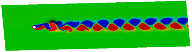
Figure 3: Instantaneous cylinder wake for flow past a stationary cylinder with a Gaussian bump in the wake at $Re=100$.

3.4 Flow Past Stationary Square and Triangular Cylinders on a Spherical Surface

The computational domain consists of a square or an equilateral triangular cylinder contour, both with edge length unity, embedded on a spherical surface of radius $R=12$. One of the edges of the square cylinder (contour) faces the upstream flow and the opposite edge faces the downstream flow. The vertical edge of the triangular cylinder (contour) faces the downstream flow. The domain size is similar to the one described in section 3.1, except that now the lengths are geodesic distances. The same boundary conditions as described in section 3.1 are employed. Reynolds number, based on the edge length, $Re=100$ is considered. Figure 4 shows the instantaneous vortex streets, along with that for the case of flat embedding surface for a reference. Qualitatively, the vortex streets on the spherical embedding surface look similar to that on the flat embedding surface. For the square cylinder case, the mean drag coefficient, RMS lift coefficient and the Strouhal number are computed to be $1.477$, $0.2$ and $0.148$, respectively. We compare them to the corresponding values for the flat embedding surface, and the relative difference is found to be $1.2$% and $0.67$%, respectively for the mean drag coefficient and the Strouhal number. The RMS lift coefficient is found to be identical. Similarly, for the triangular cylinder, the mean drag coefficient, the RMS lift coefficient and the Strouhal number are computed to be $1.77$, $0.305$ and $0.2$, respectively. The corresponding difference is found to be $2.69$%, $4.98$% and $1.96$% relative to the flat embedding surface case.

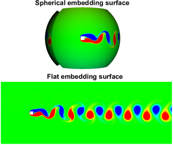
(a)

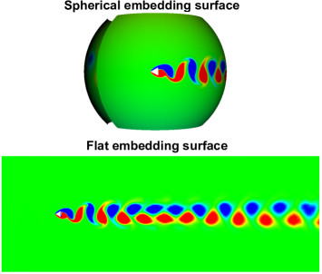
(b)

Figure 4: Instantaneous vortex streets for flow past a cylinder on a spherical embedding surface. (a) Square cylinder, (b) Triangular cylinder.

3.5 Flow Past an Airfoil

Flow over an airfoil, NACA 0012 at different angles of attack $\alpha$ is considered. The computational domain consists of the contour of the airfoil embedded on a rectangular plane. The domain lengths upstream and downstream of the airfoil leading edge are 5C and 15C, respectively, and the domain width on either side of the leading edge is 5C. Here, C stands for the chord length. The flow is set to be uniform at the inlet (the left boundary) and outflow boundary condition is applied at the outlet (the right boundary). The free stream boundary conditions are employed at the top and bottom boundaries of the domain, and a no-slip boundary condition is employed at the airfoil wall boundary. Figure 5 shows the mean pressure distribution over the upper and lower surfaces of the airfoil at $Re=1000$. The present result shows good agreement to those obtained by [46].

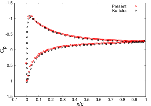
Figure 5: Mean pressure distribution for NACA0012 at an angle of attack $\alpha=9^{o}$ and $Re=1000$.

The time-averaged lift coefficient $\bar{C_{L}}$ and drag coefficient $\bar{C_{D}}$ are shown in figures 6 and 7, respectively, for different angles of attack. The results show good agreement between the present and literature results at low angles of attack with reasonable difference of aerodynamic coefficients at $15^{o}$ and $20^{o}$ angle of attack.

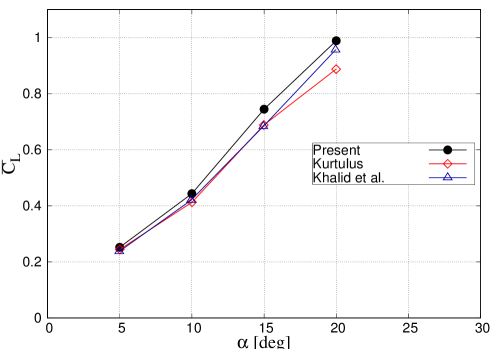
Figure 6: Mean lift coefficient $\bar{C_{L}}$ as a function of angle of attack $\alpha$, for $Re=1000$.

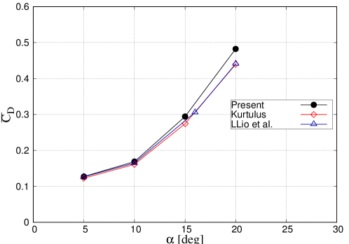
Figure 7: Mean drag coefficient $\bar{C_{D}}$ as a function angle of attack $\alpha$, for $Re=1000$.

3.6 Taylor-Green Vortices

The Taylor-Green vortices are simulated on a flat square domain of dimension [-0.5,0.5] both in $x$ and $y$ coordinate directions. The non-dimensional analytical solution for the decay of Taylor-Green vortices with time in 2D reads [47]

$$u_{x}=-\cos\left(2\pi x\right)\sin\left(2\pi y\right)e^{-8\pi^{2}t/Re},$$ (19)

$$u_{y}=\sin\left(2\pi x\right)\cos\left(2\pi y\right)e^{-8\pi^{2}t/Re},$$ (20)

where $u_{x}$ and $u_{y}$ are the $x$ and $y$ components of non-dimensional velocity respectively, $x$ and $y$ are the non-dimensional coordinates, $Re$ is the Reynolds number, and $t$ is the non-dimensional time. The Reynolds number is defined as the ratio of viscous diffusion time to the circulation (turnover) time, i.e., $Re=\frac{L^{2}/\nu}{L/V}$. Here, $L$ is the characteristic length scale, $V$ is the characteristic velocity scale, and $\nu$ is the kinematic viscosity. The circulation time $\left(L/V\right)$ is used as the characteristic time scale. At time $t=0$, the mass flux 1-form for a primal edge is determined from the integration of the normal component of velocity along the edge. The Reynolds number $Re=200$ is used for the simulations. Structured triangular meshes and Delaunay meshes of different resolutions are used for the simulations and an error convergence study is performed. Figure 8 shows the convergence with the mesh element size of the $L^{2}$-norm of the velocity 1-form (flux) error $\left\|u^{analytical}-u^{numerical}\right\|=\left[\sum_{\sigma^{1}}\left(\frac{u^{analytical}-u^{numerical}}{\left|\sigma^{1}\right|}\right)^{2}\left|\sigma^{1}\right|\left|\star\sigma^{1}\right|\right]^{1/2}$ [21] at simulation time $t=10$. Here the superscripts analytical and numerical stand for the analytical and numerical solutions, respectively. We observe that the flux error converges with a second order rate for the structured-triangular mesh, and with a rate somewhat better than first order (i.e., $1.45$) otherwise, which agrees largely with that reported in [21]. Figure 8 also shows the convergence of the $L^{2}$-norm of the velocity magnitude error. The velocity vector field was interpolated from the flux distribution using Whitney maps [21]. The velocity error converges with a rate slightly better than first order (i.e., $1.2$) for both the structured triangular mesh as well as the Delaunay mesh. For the structured triangular meshes, although the flux error converges with a second order rate, the velocity error converges at a rate slightly better than first order, due to the first order interpolation of velocity field from the flux distribution. We note that the stream function formulation [21] also exhibits similar second order flux error convergence rate for the structured-triangular meshes and first order flux error convergence rate for the otherwise unstructured meshes, and first order velocity error convergence rate for both the structured-triangular meshes as well as the unstructured meshes. For the post processing, the vorticity distribution (here, there is only one component of vorticity normal to the domain plane) was determined from the flux distribution as $\omega=\ast_{0}^{-1}\left[-\textrm{d}_{0}^{T}\right]\ast_{1}u^{\ast}$. Figure 9a shows the vorticity distribution at simulation time $t=10$. Figure 9b shows, at simulation time $t=10$, the distribution of the $y$-velocity along the horizontal domain center line along with analytical solution, and the two agree well.

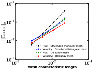
Figure 8: The convergence of the $L^{2}$-norm of the velocity 1-form (flux) and the interpolated velocity vector errors with mesh size for the Taylor-Green vortices case at time $t=10$. The dashed lines represent the slopes of the orders: (i) black: 2.0, (ii) blue: 1.2, (iii) green: 1.45, (i) red: 1.2.

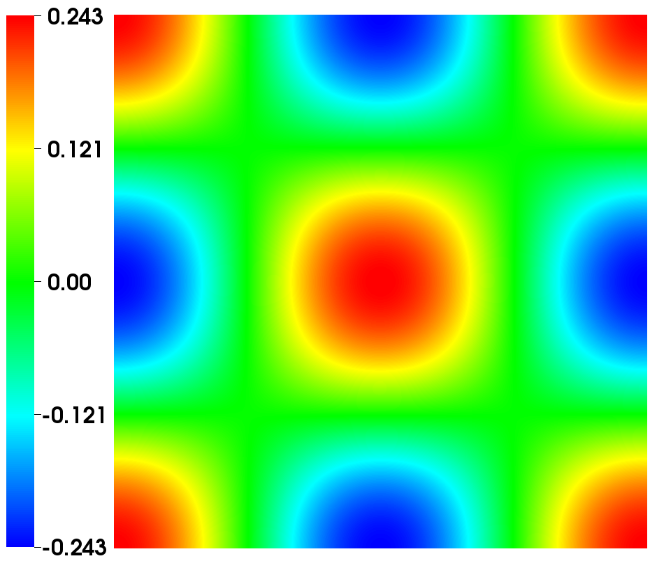
(a)

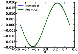
(b)

Figure 9: (a) The vorticity distribution for Taylor-Green vortices at time $t=10$. (b) The $y$-velocity distribution along the horizontal centerline at time $t=10$.

3.7 Double Periodic Shear Layer

An inviscid flow and a square domain of unit edge length is assumed. Figure 10a shows the initial flow, which is a shear layer of finite thickness with a small magnitude of vertical velocity perturbation. The expression of the initial velocity field is [48]

$$u_{x}=\begin{cases}\begin{array}[]{c}\tanh\left(\left(y-0.25\right)/\rho\right)\textrm{ for }y\leq 0.5\\ \tanh\left(\left(0.75-y\right)/\rho\right)\textrm{ for }y>0.5\end{array}\end{cases}$$ (21)

$$u_{y}=\delta\sin\left(2\pi x\right)$$ (22)

with $\rho=1/30$ and $\delta=0.05$. Similar to the case of Taylor-Green vortices (section 3.6), the initial mass flux 1-forms are approximated from the integration of the normal component of velocity along the edges. Periodic boundary conditions are imposed at all domain boundaries. Four mesh resolutions consisting of structured-triangular meshes with number of elements equal to $8192$, $32768$, $131072$ and $524288$ are employed. A time step of $\Delta t=0.001$ is used. Figure 10 shows the evolution of the vorticity field with time, using the finest mesh. At time $t=0.8$, two well resolved vortices appear. Similar to that reported in Mohamed et al. [21], the shear layer connecting the coherent vortices becomes thinner with time and within a finite time interval reach the resolution of the mesh after which dispersion error manifests as mesh level oscillations. The vorticity distribution plots in figure 10 exhibit similarities with that reported previously by Mohamed et al. [21], and Bell et al. [48].

Figure 10d the convergence of the kinetic energy relative error $\left(\frac{\textrm{KE}\left(0\right)-\textrm{KE}\left(t\right)}{\textrm{KE}\left(0\right)}\right)$ with the mesh size at time $t=2.0$. Here, the total kinetic energy $\left(\textrm{KE}\right)$ is calculated as $\frac{1}{2}\int_{\Omega}\mathbf{v}\cdot\mathbf{v}d\Omega$, where the integration is performed over the entire simulation domain, where the velocity vector $\left(\mathbf{v}\right)$ is calculated in each triangular element via Whitney map interpolation, as discussed before. As expected, the kinetic energy relative error converges in a second order fashion with the mesh size. It is worth noting that the stream function formulation [21] also exhibits similar second order convergence rate of the kinetic energy relative error. Kinetic energy relative error is $0.2\%$ for the coarsest mesh (equivalent to $64\times 64$ Cartesian mesh) and it is only $0.0039\%$ for the finest mesh (equivalent to $512\times 512$ Cartesian mesh). It is $0.06\%$ for the mesh with $32768$ triangular elements (equivalent to a $128\times 128$ Cartesian mesh), almost one order of magnitude lower than a second order collocated mesh scheme [48] using almost the same mesh size.

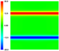
(a)

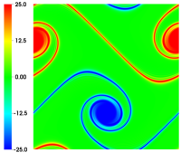
(b)

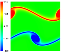
(c)

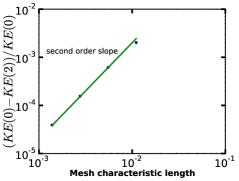
(d)

Figure 10: Double periodic shear layer case. Vorticity magnitude distribution at (a) $t=0$, (b) $t=0.8$, (c) $t=1.2$. (d) kinetic energy relative error at $t=2$.

3.8 Motion of Harmonic Waves on a Rotating Sphere

There exists a stationary solution to the motion of harmonic waves in the Earth’s atmosphere. These waves are the so-called Rossby waves. The stationary solution is [49]

$$\psi\left(\phi,\theta\right)=A\sin m\phi P_{l}^{m}\left(\cos\theta\right)-BR^{2}\cos\theta,$$ (23)

where, $\psi$ is the stream function, $B=\frac{2\Omega}{l\left(l+1\right)-2}$, $\phi$ is longitude, $\theta$ is the colatitude angle, $A$ is an arbitrary constant, $P_{l}^{m}$ is associated Legendre polynomial of degree $l$ and order $m$, $R$ is earth’s radius, and $\Omega$ is the rate of earth’s rotation. An inviscid flow and $f=2\Omega\cos\theta$ are considered. The stream function distribution is shown in figure 11 for $A=200$, $l=7$, $m=6$, $R=6.371\times 10^{6}$, and $\Omega=7.2921\times 10^{-5}$. Figure 11a shows the stationary solution at time $t=0$, and 11b shows the one at time $t=3.144\times 10^{6}$ s or $36.39$ days. There is no distortion of the stream function distribution and the stationary solution is preserved. However, there is a westward phase displacement of $28.6^{\circ}$ longitude after $36$ days. ($5.7^{\circ}$ longitude after 7 days). Similar westward phase displacement of $7^{\circ}$ longitude after $8$ days has been reported in [50].

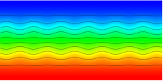
(a)

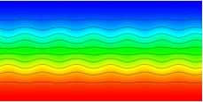
(b)

Figure 11: Stream function distribution for the motion of harmonic waves on a rotating sphere case. (a) $t=0$, (b) $t=36.39$ days.

Figure 12 shows various inviscid invariants as a function of time, and demonstrates conservation of these invariants for an extended period of time. It is observed that energy-preserving time integration has a superior conservation of total kinetic energy and the total enstrophy as compared to the Euler first order time integration. The total kinetic energy is already defined in section 3.7. The total enstrophy is calculated as $\frac{1}{2}\int_{\Omega}\omega^{2}d\Omega$, where the integration is performed over the entire simulation domain, and $\omega$ is the vorticity.

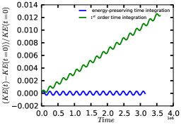
(a)

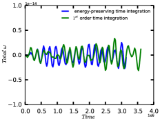
(b)

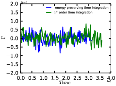
(c)

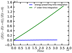
(d)

Figure 12: Inviscid invariants as a function of time for the motion of harmonic waves on a rotating sphere case. (a) Total relative kinetic energy, (b) Total vorticity, (c) Total circulation, (d) Total relative enstrophy.

4 Conclusions

We presented a primitive variable DEC formulation of Navier-Stokes equations on surface simplicial meshes. Here, the mass flux 1-forms at all mesh primal edges, and the dynamic pressure 0-forms at the mesh dual nodes (triangle circumcenters) are the degrees of freedom. The discrete operators emerging from the DEC discretization are discussed. Two time integration schemes, i.e., Euler first order, and energy-preserving, are implemented. The Coriolis force is incorporated to facilitate the use of the method to study flows on rotating surfaces. The method exhibits second order flux error convergence rate with the mesh size for the structured triangular meshes, and a rate somewhat better than first order (i.e., 1.45) for unstructured meshes. Moreover, the method exhibits slightly better than first order (i.e., 1.2) error convergence rate with the mesh size for the interpolated velocity vector for both the structured triangular as well as unstructured meshes. The method exhibits second order kinetic energy relative error convergence rate with mesh size for inviscid flows. The method preserves a stationary state for the flow on a rotating sphere over an extended period of time. The energy-preserving time integrator exhibits superior conservation of inviscid invariants such as total kinetic energy and total enstrophy for an extended period of time.

References

Appendix

Primer on Discrete Exterior Calculus (DEC)

The calculus of differential forms is dubbed exterior calculus. While vector calculus deals with scalars, vectors and tensors, exterior calculus deals with differential forms ($k$-forms). Perot et al. [51] describes differential forms, with a view point of their applications to science and engineering, and is largely referred to in the ensuing discussion. A differential form can be regarded as “the things which occur under integral signs” [52]. For example, for a line integral of a vector $u$, $\int u\cdot\mathbf{dl}$, $u\cdot\mathbf{dl}$ is a 1-form $u^{1}$. Similarly, a 2-form $a^{2}=\mathbf{a}\cdot\mathbf{dA}$ appears in surface integrals, a 3-form $b^{3}=bdV$ appears in volume integrals, and since a 0-integral is trivial, a 0-form $p^{0}$ is a scalar function. Here, the superscript on the form is the dimension of the form. On the other hand, the discrete forms are the entire integral quantities. For example, integration of a vector $u$ over a mesh edge $\int u\cdot\mathbf{dl}$ is a discrete 1-form $u^{1}$. Similarly, surface integral $\int\mathbf{a}\cdot\mathbf{dA}$ over a mesh face represents a discrete 2-form $a^{2}$, and a discrete 3-form is the volume integral $b^{3}=\int bdV$ on a cell volume. Since the integration over a point is trivial and it just returns the value of the integrand at that point, a discrete 0-form is just a scalar field value at a mesh vertex/node. The perception of discrete 0-form and that of the discrete 1-form remain essentially the same for two-dimensional (2D) and three-dimensional (3D) spaces. However, since the mesh cells are represented by areas in 2D, the discrete 2-form is a cell average integral of a scalar field in 2D rather than integral of a vector field on a mesh face as in 3D. The confining space dimension is the highest dimension of a form. Therefore, there does not exist a 3-form in 2D, and the 2-form essentially behaves like the 3-form does in 3D. Other key concepts are the exterior derivative $\left(\textrm{d}\right)$, the Hodge star operator $\left(\ast\right)$, and the exterior product or wedge product $\left(\wedge\right)$. The exterior derivative implies multidimensional differentiation, and is a generalization of the usual curl, divergence and gradient operations of calculus. It operates on a form and results in to the next higher dimensional form. The gradient of a scalar in 3D, i.e., $\nabla q=\mathbf{p}$ in vector calculus is equivalent to $\textrm{d}q^{0}=p^{1}$ in exterior calculus. Here, the 1-form $p^{1}$ best represents the resulting vector $\mathbf{p}$. The curl of a vector, $\nabla\times u=\mathbf{a}$ is equivalent to $\textrm{d}u^{1}=a^{2}$. The resulting vector $\mathbf{a}$ (in vector calculus) is represented as a 2-form (in exterior calculus). The divergence of a vector, $\nabla\cdot u=b$ is equivalent to $\textrm{d}u^{2}=b^{3}$, resulting in to a 3-form which is a scalar. In 2D, gradient $\nabla,$ and 2D curl $\nabla\times_{2D}$ are the only primary differentiation operations, and the divergence does not add any useful content. The gradient of a scalar looks the same as in 3D, i.e., it is equivalent to the exterior derivative operating on a 0-form, and implies the difference between two node values / discrete 0-forms. The curl of a vector lying in a plane , $\nabla\times_{2D}u=\frac{\partial u_{y}}{\partial x_{x}}-\frac{\partial u_{x}}{\partial x_{y}}$, is equivalent to a 2-form resulting from the application of an exterior derivative to a 1-form (on an edge). The discrete exterior derivative $\textrm{d}_{0}$ operates on primal 0-forms and results in to primal 1-forms, and the discrete exterior derivative $\textrm{d}_{1}$ operates on primal 1-forms and results in to primal 2-forms. Similarly, (in 2D) the discrete exterior derivative $\left[-\textrm{d}_{0}^{T}\right]$ (the negative sign is due to the adopted mesh orientation convention) operates on dual 0-forms and results in to dual 1-forms and the discrete exterior derivative $\textrm{d}_{1}^{T}$ operates on dual 1-forms and results in to dual 2-forms. The Hodge star operator has a metric term incorporated in it. The Hodge star operating on a form in one dimension (e.g., $k$) results in to a form in the reflected dimension ($N-k$), i.e., $\ast a^{k}=b^{N-k}$, where $N$ stands for the space dimension. In 3D, Hodge star on a 0-form (scalar value at a point / node) results in to a 3-form (cell average of scalar), and vice-versa. Applying Hodge star to a 1-form (vector component along a line) results in a 2-form (vector component normal to a face) and vice-versa. In practice, this implies that a discrete Hodge star operator transfers the forms on a mesh to a dual mesh (as well as changes their dimension). One need to identify which dual mesh is being used for the definition of the discrete Hodge star matrices, since every well formed mesh has an infinite number of well formed dual meshes. The median dual mesh (barycentric dual mesh), and the voronoi dual mesh (circumcentric dual mesh) are the examples of dual meshes for unstructured (triangular or tetrahedral) primary meshes. The discrete Hodge star $\left(\ast_{0}\right)$ operating on cell node (vertex) values (0-forms) of a tetrahedral mesh results in cell average values (dual 3-forms) for the surrounding Voronoi cells. Similarly, the inverse operator $\left(\ast_{1}^{-1}\right)$ operates on 1-forms lying on a dual mesh edge (i.e., on the line between circumcenters of two adjacent primal cells), and results in to 2-forms on the primal mesh (normal flux values on the cell faces). In 2D, a discrete $\ast_{0}$ operates on mesh vertex values (primal 0-forms), and results in to Voronoi cell values (dual 2-forms). The operation $\ast_{0}^{-1}$ transfers the cell average values (dual 2-forms) to mesh vertex values (primal 0-forms). The discrete $\ast_{1}$ operator transfers the primal 1-forms (primal edge values) to dual 1-forms (dual edge values). On the other hand, The discrete $\ast_{1}^{-1}$ operator transfers the dual 1-forms (dual edge values) to primal 1-forms (primal edge values). The wedge product of two forms implies multiplication of the forms. The dimension of the resultant form is the sum of the dimensions of the two forms in the wedge product, i.e., $a^{j}\wedge b^{k}=c^{j+k}$ for $j+k\leq N$, with a property $a^{j}\wedge b^{k}=\left(-1\right)^{jk}b^{k}\wedge a^{j}$. The wedge product is also associative, i.e., $\left(a^{j}\wedge b^{k}\right)\wedge c^{l}=a^{j}\wedge\left(b^{k}\wedge c^{l}\right)$ for $j+k+l\leq N$. In 3D, the wedge product implies a regular multiply, a dot-product, or a cross-product depending on the dimension of the two forms involved in the wedge product. The wedge product implies a regular multiplication, if either operand is a scalar 0-form. When one of the operands is a 1-form and the other is a 2-form the wedge product implies a dot product of them. The wedge product of two 1-forms implies cross product on the vector proxies of the forms, resulting in a 2-form. In 2D, the wedge product of two forms implies either a regular multiplication or a 2D cross product of the forms. Similar to 3D, if either operand is a 0-form, a regular multiply is implied. For the two forms $a^{1}$ and $b^{1}$ associated with the vectors $\mathbf{a}$ and $\mathbf{b}$, respectively, the wedge product $a^{1}\wedge b^{1}$ is equivalent to $\mathbf{a}\times_{2D}\mathbf{b}=a_{x}b_{y}-a_{y}b_{x}$. Using integral quantities / discrete forms as the primary unknowns for a numerical method transforms any continuous PDE system in to a discrete algebraic system such that all errors/approximations occur at the algebraic level only and not in the approximation of the differential operators of the PDE [4]. Thus, DEC can mimic physical and mathematical properties of the continuous PDE system. Moreover, DEC being coordinate independent, it is a more convenient numerical tool to investigate flows over arbitrary curved surfaces/manifolds. The DEC implementation requires a primal simplicial complex (triangular mesh in 2D or tetrahedral mesh in 3D), along with a dual mesh associated to it (usually circumcentric). In 2D, the primal simplicial complex consists of the set of nodes, edges, and triangles, and the dual mesh consists of dual polygons, edges and nodes associated with the primal mesh objects. DEC discretization of a physical problem expresses the physical fields discretely as scalars representing the integration of these $k$-forms on $k$-dimensional primal/dual mesh objects as already mentioned above. A few representative DEC references include [52, 53, 11, 14, 12, 15, 20, 13, 18, 51, 21, 19].

References

- Marsden and West [2001] J. E. Marsden, M. West, Discrete mechanics and variational integrators, Acta Numerica 10 (2001) 357–514.
- Hairer et al. [2006] E. Hairer, C. Lubich, G. Wanner, Geometric numerical integration: structure-preserving algorithms for ordinary differential equations, volume 31, Springer Science & Business Media, 2006.
- Arnold et al. [2007] D. N. Arnold, P. B. Bochev, R. B. Lehoucq, R. A. Nicolaides, M. Shashkov, Compatible spatial discretizations, volume 142, Springer Science & Business Media, 2007.
- Perot and Subramanian [2007] J. B. Perot, V. Subramanian, Discrete calculus methods for diffusion, Journal of Computational Physics 224 (2007) 59–81.
- Poincaré et al. [1887] H. Poincaré, et al., Sur les résidus des intégrales doubles, Acta Mathematica 9 (1887) 321–380.
- Cartan [1899] É. Cartan, Sur certaines expressions différentielles et le problème de pfaff, in: Annales scientifiques de l’École Normale Supérieure, volume 16, 1899, pp. 239–332.
- Goursat [1915] E. Goursat, Sur certains systèmes d’équations aux différentiels totales et sur une généralisation du problème de pfaff, in: Annales de la Faculté des sciences de Toulouse: Mathématiques, volume 7, 1915, pp. 1–58.
- Abraham [1932] M. Abraham, The classical theory of electricity and magnetism (1932).
- Cartan [1946] E. Cartan, Leçons sur la géométrie des espaces de riemann (2-nd. ed.), Gauthier-Villars, Paris (1946).
- De Rham [1955] G. De Rham, Variétés différentiables. formes, courants, formes harmoniques. actualits sci. ind., no. 1222, publ, Inst. Math. Univ. Nancago III., Hermann, Paris (1955).
- Hirani [2003] A. N. Hirani, Discrete exterior calculus, Ph.D. thesis, California Institute of Technology, 2003.
- Desbrun et al. [2005] M. Desbrun, A. N. Hirani, M. Leok, J. E. Marsden, Discrete exterior calculus, arXiv preprint math/0508341 (2005).
- Desbrun et al. [2008] M. Desbrun, E. Kanso, Y. Tong, Discrete differential forms for computational modeling, in: Discrete differential geometry, Springer, 2008, pp. 287–324.
- Desbrun et al. [2003] M. Desbrun, A. N. Hirani, J. E. Marsden, Discrete exterior calculus for variational problems in computer vision and graphics, in: Decision and Control, 2003. Proceedings. 42nd IEEE Conference on, volume 5, IEEE, 2003, pp. 4902–4907.
- Grinspun et al. [2006] E. Grinspun, M. Desbrun, K. Polthier, P. Schröder, A. Stern, Discrete differential geometry: an applied introduction, ACM Siggraph Course 7 (2006) 1–139.
- Elcott et al. [2007] S. Elcott, Y. Tong, E. Kanso, P. Schröder, M. Desbrun, Stable, circulation-preserving, simplicial fluids, ACM Transactions on Graphics (TOG) 26 (2007) 4–es.
- Mullen et al. [2009] P. Mullen, K. Crane, D. Pavlov, Y. Tong, M. Desbrun, Energy-preserving integrators for fluid animation, ACM Trans. Graph. 28 (2009) 38.
- Crane et al. [2013] K. Crane, F. De Goes, M. Desbrun, P. Schröder, Digital geometry processing with discrete exterior calculus, in: ACM SIGGRAPH 2013 Courses, 2013, pp. 1–126.
- de Goes et al. [2016] F. de Goes, M. Desbrun, M. Meyer, T. DeRose, Subdivision exterior calculus for geometry processing, ACM Transactions on Graphics (TOG) 35 (2016) 1–11.
- Hirani et al. [2008] A. N. Hirani, K. B. Nakshatrala, J. H. Chaudhry, Numerical method for darcy flow derived using discrete exterior calculus, arXiv preprint arXiv:0810.3434 (2008).
- Mohamed et al. [2016] M. S. Mohamed, A. N. Hirani, R. Samtaney, Discrete exterior calculus discretization of incompressible navier–stokes equations over surface simplicial meshes, Journal of Computational Physics 312 (2016) 175–191.
- Nitschke et al. [2017] I. Nitschke, S. Reuther, A. Voigt, Discrete exterior calculus (dec) for the surface navier-stokes equation, in: Transport Processes at Fluidic Interfaces, Springer, 2017, pp. 177–197.
- Mohamed et al. [2018] M. S. Mohamed, A. N. Hirani, R. Samtaney, Numerical convergence of discrete exterior calculus on arbitrary surface meshes, International Journal for Computational Methods in Engineering Science and Mechanics (2018) 1–13.
- Zhang et al. [2002] X. Zhang, D. Schmidt, B. Perot, Accuracy and conservation properties of a three-dimensional unstructured staggered mesh scheme for fluid dynamics, Journal of Computational Physics 175 (2002) 764–791.
- Frank and Reich [2003] J. Frank, S. Reich, Conservation properties of smoothed particle hydrodynamics applied to the shallow water equation, BIT Numerical Mathematics 43 (2003) 41–55.
- Perot [2011] J. B. Perot, Discrete conservation properties of unstructured mesh schemes, Annual review of fluid mechanics 43 (2011) 299–318.
- Nicolaides [1989] R. Nicolaides, Flow discretization by complementary volume techniques, in: 9th Computational Fluid Dynamics Conference, 1989, p. 1978.
- Hall et al. [1991] C. Hall, J. Cavendish, W. Frey, The dual variable method for solving fluid flow difference equations on delaunay triangulations, Computers & fluids 20 (1991) 145–164.
- Nicolaides [1992] R. A. Nicolaides, Direct discretization of planar div-curl problems, SIAM Journal on Numerical Analysis 29 (1992) 32–56.
- Perot [2000] B. Perot, Conservation properties of unstructured staggered mesh schemes, J. Comput. Phys. 159 (2000) 58–89.
- Bauer [2013] W. Bauer, Toward goal-oriented R-adaptive models in geophysical fluid dynamics using a generalized discretization approach, Ph.D. thesis, Hamburg University Hamburg, 2013.
- Mohamed et al. [2018] M. S. Mohamed, A. N. Hirani, R. Samtaney, Numerical convergence of discrete exterior calculus on arbitrary surface meshes, International Journal for Computational Methods in Engineering Science and Mechanics 19 (2018) 194–206. URL: https://doi.org/10.1080/15502287.2018.1446196. doi:10.1080/15502287.2018.1446196. arXiv:https://doi.org/10.1080/15502287.2018.1446196.
- Shi et al. [2004] J. M. Shi, D. Gerlach, M. Breuer, G. Biswas, F. Durst, Heating effect on steady and unsteady horizontal laminar flow of air past a circular cylinder, Physics of Fluids 16 (2004) 4331–4345. doi:10.1063/1.1804547.
- Russell and Wang [2003] D. Russell, Z. J. Wang, A cartesian grid method for modeling multiple moving objects in 2d incompressible viscous flow, Journal of Computational Physics 191 (2003) 177–205.
- Kawaguti [1953] M. Kawaguti, Numerical solution of the navier-stokes equations for the flow around a circular cylinder at reynolds number 40, Journal of the Physical Society of Japan 8 (1953) 747–757.
- Le et al. [2006] D. Le, B. C. Khoo, J. Peraire, An immersed interface method for viscous incompressible flows involving rigid and flexible boundaries, Journal of Computational Physics 220 (2006) 109–138.