Artificial coherent states of light by multi-photon interference in a single-photon stream

Abstract

Coherent optical states consist of a quantum superposition of different photon number (Fock) states, but because they do not form an orthogonal basis, no photon number states can be obtained from it by linear optics. Here we demonstrate the reverse, by manipulating a random continuous single-photon stream using quantum interference in an optical Sagnac loop, we create engineered quantum states of light with tunable photon statistics, including approximate weak coherent states. We demonstrate this experimentally using a true single-photon stream produced by a semiconductor quantum dot in an optical microcavity, and show that we can obtain light with $g^{(2)}(0)\rightarrow 1$ in agreement with our theory, which can only be explained by quantum interference of at least 3 photons. The produced artificial light states are, however, much more complex than coherent states, containing quantum entanglement of photons, making them a resource for multi-photon entanglement.

Coherent states of light are considered to be the most classical form of light, but expressed in photon number (Fock) space, they consist of a complex superposition of a number of photon number (Fock) states. Because coherent states are non-orthogonal, it is not possible with linear-optical manipulation and superposition of coherent states to obtain pure photon number (Fock) states. The opposite is possible in principle, for instance by attenuating high-$N$ photon number states one could synthesize coherent states. However, high-$N$ Fock states are not readily available, but recently high-quality sources of single-photon ($N=1$) states became accessible based on optical nonlinearities on the single-photon level. In particular, by using semiconductor quantum dots in optical microcavities Santori2002 , single-photon sources with high brightness, purity, and photon indistinguishability were realized He2013 ; Somaschi2016 ; Ding2016 ; Snijders2018 . Under loss, in contrast to higher-$N$ Fock states, single-photon streams never loose their quantum character since single photons cannot be split, loss reduces only the brightness. Single photons are an important resource for quantum information applications Knill2001 .

In order to synthesize more complex quantum states of light, multiple identical single-photon streams can be combined using beamsplitters, where unavoidably quantum interference appears, the well-known Hong-Ou-Mandel (HOM) effect Hong1987 . This effect leads to photon bunching if the incident photons are indistinguishable, therefore enables the production of higher photon number states but only probabilistically. HOM interference is also used for characterization of the photon indistinguishability of single-photon sources Santori2002 , which is done mostly in the pulsed regime where detector time resolution is not an issue. The regime of a continuous but random stream of single photons has been explored much less in this aspect, HOM interference with continuous random stream of true single photons has been observed in Refs. Patel2008 and Proux2015 . The HOM effect can also be used to entangle photons; in combination with single-photon detection and post-selection, it also can act as a probabilistic CNOT gate Larque2008 ; Fattal2004 ; Knill2001 .

Here we make use of HOM interference in a Sagnac-type delay loop with a polarizing beamsplitter (Fig. 1), where HOM interference happens at a half-wave plate in polarization space . Similar setups are proposed for boson sampling Motes2014 ; He2017 and used for producing linear photonic cluster states Megidish2012 ; Pilnyak_PRA17 ; Istrati2020 , an emerging resource for universal quantum computation Knill2001 ; Raussendorf2001 ; Walther2005 . Since we operate with a random but continuous single-photon stream, the repeated quantum interference and enlargement of the spatio-temporal superposition leads to an infinitely long quantum superposition. By tuning the photon indistinguishability we observe, in agreement with our theoretical model, photon correlations approaching that of coherent light ($g^{(2)}(0)\rightarrow 1$), and from our theoretical model, we deduce that the photon number distribution indeed corresponds to coherent light, more precisely weak coherent light with a mean photon number $\bar{n}\approx 0.2$.

Experimentally, as an efficient single-photon source, we use a self-assembled InGaAs/GaAs quantum dot (QD) embedded in polarization-split micropillar cavity grown by molecular beam epitaxy Snijders2018 ; Snijders2020 . The QD layer is embedded in a p-i-n junction, separated by a 27 nm-thick tunnel barrier from the electron reservoir, to enable tuning of the QD resonance around 935 nm by the quantum-confined Stark effect. The QD transition with a cavity-enhanced lifetime of $\tau_{r}=130\pm 15\,\mathrm{ps}$ is resonantly excited with a continuous-wave laser, which is separated by a cross-polarization scheme Snijders2020 from the single photons that are collected in a single-mode fiber. This linearly ($H$) polarized single-photon stream $\Psi_{in}$ is then brought by WP1 ($22.5^{\circ}$) in a superposition of two polarization modes; $H$-polarized photons enter the 1 m long free-space delay-loop wherein WP2 ($22.5^{\circ}$) brings them again in a superposition, only $H$-polarized photons are transmitted from the loop towards the detection part. Detection is done with a standard Hanbury Brown and Twiss (HBT) setup with a non-polarizing beamsplitter, after which the photons are coupled into multi-mode fibers (coupling efficiency $\sim 90$%) and detected with silicon avalanche photon detectors (APDs, 25% efficiency) and analyzed with a time-correlated single-photon counting computer card. With motorized half-wave plates followed by a fixed linear polarizer before each multi-mode fiber coupler, the setup allows to distinguish correlations between photons from the loop ($g_{HH}^{(2)}(\tau)$), only directly from the source ($g_{VV}^{(2)}(\tau)$), and to analyze cross-correlations between photons from the loop and source $g_{VH}^{(2)}(\tau)$. Note that measurement in $VV$ polarization is equivalent to a standard $g^{(2)}(\tau)$ measurement of the single-photon source and can be used to obtain a reference without changing the experimental setup. We have chosen a beam waist of $0.50$ mm inside the loop in order to reduce diffraction loss; the total round-trip transmission $\eta_{L}$ is $\sim 90\%$. Further, we use active phase-stabilization of the loop length by using a mirror on a piezoelectric actuator (Fig. 1(b)) and a frequency-stabilized He-Ne laser entering the loop through a doubly polished mirror, this is needed because weak pure single-photon states interfere phase-sensitively Loredo2019 .

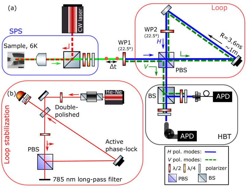
Figure 1: Experimental setup - (a) Photons from the single-photon source (SPS) are diagonally polarized by WP1 before sent to the loop setup consisting of a polarizing beamsplitter and half-wave plate WP2 at $22.5^{\circ}$. Light from the loop setup is analyzed with the polarization-resolved HBT setup. Panel (b) shows the interferometric loop length stabilization.

We operate the QD single-photon source with relatively high excitation power ($\sim 50$ nW) to obtain a bright single-photon stream (detected single-photon detection rate of $200\,\mathrm{kHz}$), with the consequence that unwanted effects produce a broad correlation peak superimposed to $g^{(2)}(\tau)$. In order to correctly take this into account in our model, we first measure in $VV$ detector configuration the source correlations (Fig. 2(a)) and model it using a three-level system Kitson_1998 ; Kurtsiefer_2000 , where $\tau_{B}$ is the lifetime of the additional dark state:

$$g_{3L}^{(2)}(\tau)=1-(1+a)\exp(-|\tau|/\tau_{r})+a\exp(-|\tau|/\tau_{B}).$$ (1)

Further, for comparison to experimental results with expected $g^{(2)}(0)$ below 0.1 Snijders2018 , the theoretical data are convolved with a Gaussian instrument response function (IRF) of our single-photon detectors with $FWHM=0.523\,\mathrm{ns}$ Snijders2016 , limiting the smallest detectable $g^{(2)}(0)\approx 0.63$. From fitting the model to the experimental data, we obtain a bunching strength $a=0.24\pm 0.03$ and $\tau_{B}=5.2\pm 0.3\,\mathrm{ns}$, similar time scales were observed before Davanco2014 .

To start building up a theoretical model and to characterize the delay loop, we now measure in $VH$ detection configuration the cross-correlation function between photons directly from source and photons from the delay loop $g_{VH}^{(2)}(\tau)$, shown in Fig. 2(b). The $V$ detector is connected to the start trigger input of a correlation card and the $H$ detector to the stop channel, therefore the measured correlation $g_{VH}^{(2)}(\tau)$ is as expected asymmetric around $\tau=0$. Considering an $H$-polarized photon entering the loop, WP2 transforms it into an $\frac{1}{\sqrt{2}}\left(|H\rangle+|V\rangle\right)$ diagonally polarized state. The $H$-polarized part of the state leaves the loop via the polarizing beamsplitter, while the $V$ part remains in the loop and is transformed by WP2 into $\frac{1}{\sqrt{2}}\left(|H\rangle-|V\rangle\right)$, this process is repeating itself infinitely. In the case of a limited amount of photons in well-defined time bins, the output can easily be described, the chance that a photon leaves the loop after $r$ round trips is $\left(\nicefrac{{\eta_{L}}}{{2}}\right)^{r}$ Pittman2002 . In our case of a random single-photon stream, the case is more complex as we describe the light stream by correlation functions which we also measure experimentally.

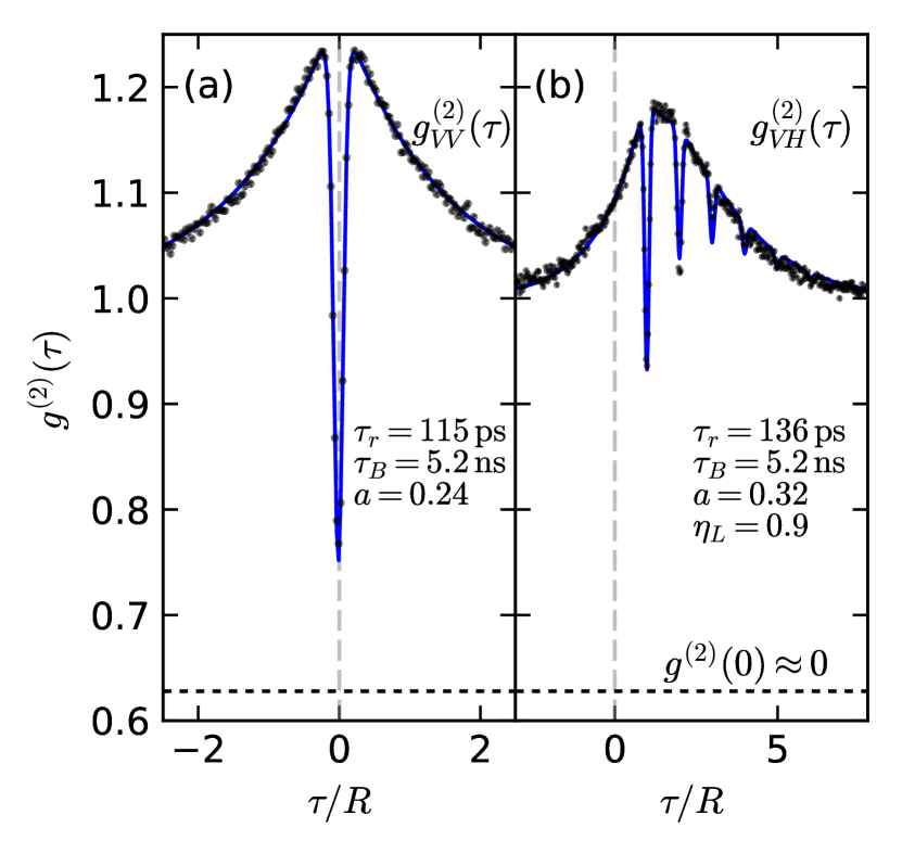
Figure 2: Characterization of the single-photon source (a) and loop setup (b), experimental data has been accumulated over 3 hours; solid lines show the model calculations. In (a) the three-level model is fitted to the experimental $g_{VV}^{(2)}(\tau)$ data to obtain the single-photon source and detector parameters used throughout the paper. Panel (b) shows $VH$ correlations between photons directly from the source and from the loop, confirming the validity of our model.

In order to predict $g_{VH}^{(2)}(\tau)$ theoretically, we use as an approximation that maximally two photons are in the system, which we prove later to be appropriate here. We obtain for the detected state for two incident photons with delay $\Delta t\neq 0$ (it is a single-photon source) a weighted superposition of single-photon streams shifted by time $r\cdot R$, where $r$ is the round-trip number and $R$ the round-trip delay (see Supplemental Information ):

$$|\Psi_{VH}\rangle=\sum_{\Delta t\neq 0}V^{\dagger}\left[\sqrt{\frac{\eta_{L}}{2}}H_{R+\Delta t}^{\dagger}+\sum_{r\geq 2}\left(-\sqrt{\frac{\eta_{L}}{2}}\right)^{r}H_{r\cdot R+\Delta t}^{\dagger}\right]|0\rangle.$$ (2)

The state is written in terms of photon creation operators $V_{t}^{\dagger}$ and $H_{t}^{\dagger}$, where the polarization mode is represented by the capital letter, the detection time is given in the subscript. Assuming a source continuously emitting perfect single photons, we can derive from the two-photon state an analytical expression for $g_{VH}^{(2)}(\tau)$:

$$g_{VH}^{(2)}(\tau)=1-\sum_{m>0}\left(\frac{\eta_{L}}{2}\right)^{m}\left(1-g_{3L}^{(2)}(\tau-m\cdot R)\right).$$ (3)

Here, photons with $\Delta t=z\cdot R,z\in\mathbb{Z}$ are correlated by the loop and create dips in $g_{VH}^{(2)}(\tau)$ for $\tau=m\cdot R$ where $m\in\mathbb{N}$ iterates over round-trips. We observe good agreement between theory and experimental data in Fig. 2(b). Note that also the shifted broad peak originating from strong driving is correctly reproduced.

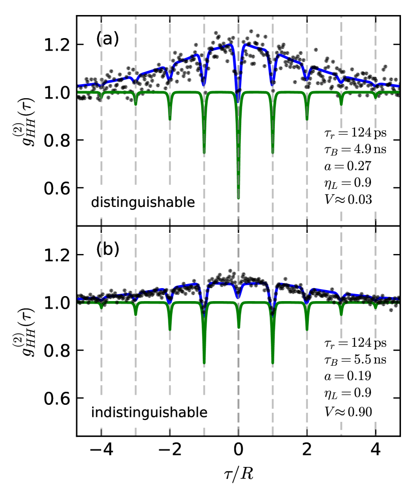
Figure 3: Photon correlations $g_{HH}^{(2)}(\tau)$ (symbols) for misaligned loop (a, $V\approx 0.03$, distinguishable photons) and aligned loop (b, $V\approx 0.9$, indistinguishable photons) compared to the model predictions (blue curves). Raw coincidence counts corresponding to $g_{HH}^{(2)}(\tau)=1$ were 880 (a) and 9700 (b). The green curves show the model results for the case without spectral diffusion.

Finally, we investigate the correlations of photons emerging from the loop by measuring $g_{HH}^{(2)}(\tau)$, shown in Fig. 3. We find that $g_{HH}^{(2)}(\tau=0)$ is now highly sensitive to the indistinguishability or wave function overlap $M$ of consecutive photons produced by the quantum dot, which we can tune experimentally simply by changing the spatial alignment of the delay loop. Assuming a perfect single-photon source, the wave function overlap $M$ is equal to the interferometric visibility $V$, see the Supplemental section .3 for details Note2 . The model for the case of distinguishable photons, shown in Fig. 3(a), can be calculated again in the two-photon picture Note2 , and we obtain

$$g_{HH}^{(2)}(\tau)= 1-\frac{2\eta_{L}}{4-\eta_{L}^{2}}\sum_{m\in\mathbb{Z}\backslash\left\{0\right\}}\left(\frac{\eta_{L}}{2}\right)^{|m|}\left(1-g_{3L}^{(2)}(\tau-m\cdot R)\right)$$ (4)

$$-\left(1-g_{HH}^{(2)}(0)\right)\left(1-g_{3L}^{(2)}(\tau)\right),$$

where the value of $g_{HH}^{(2)}(0)$ has to be calculated using full quantum state propagation which we describe now.

The delay loop leads to quantum interference of photons at different times in the incident single-photon stream, and HOM photon bunching occurring at WP2 produces higher photon number states in a complex quantum superposition. We have developed a computer algorithm that can simulate $g_{HH}^{(2)}(0)$, see the Supplemental Information section .2 for details Note2 . For the results shown here, we take up to 20 photons or loop iterations into account to approximate the experiment with a continuous photon stream. For completely distinguishable photons we obtain $g_{HH}^{(2)}(0)=0.49$ (corrected for dark state dynamics), which agrees well with the experimentally observed correlations in Fig. 3(a).

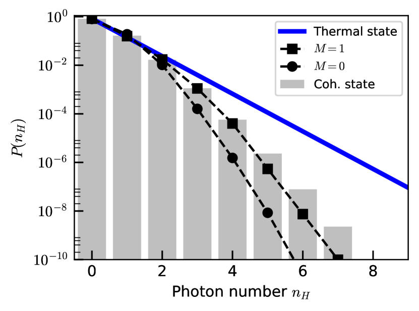
Figure 4: Comparison of the photon number distribution of a weak coherent state (bars) and thermal state (through blue line) with same mean photon number $\overline{n}\approx 0.2$, to the results from our theoretical model (squares for the case of indistinguishable photons, $M=1$, and circles for the case of distinguishable photons, $M=0$). A fixed round-trip loss of 0.1 is included in both cases. The artificial state matches best to the weak coherent light state.

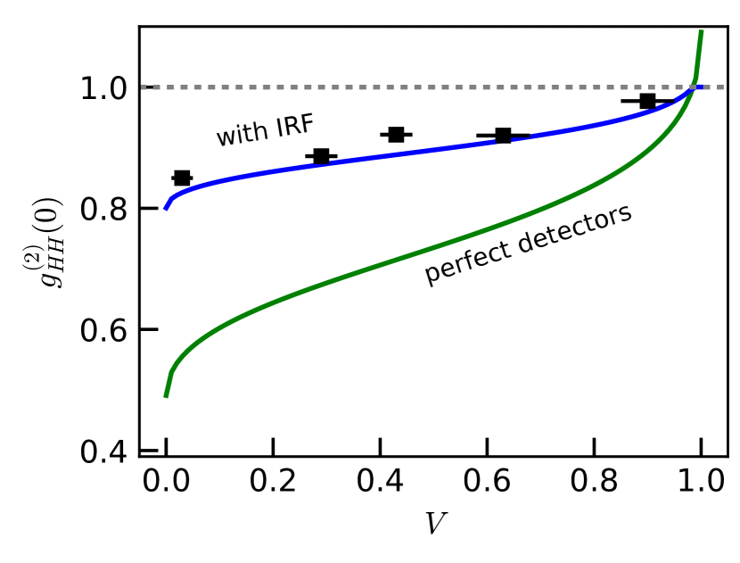
Figure 5: Experimental $g_{HH}^{(2)}(0)$ (black squares), corrected for dark state dynamics, compared to our theoretical expectations (blue line, convolved with IRF) as a function of the photon indistinguishability or wave-function overlap, expressed by the visibility $V$. Light with coherent photon statistics is obtained for $V\rightarrow 1$. The green line shows the expected results for detectors with perfect timing resolution. Results include a fixed round-trip loss of 0.1.

For the case of indistinguishable photons with maximal wave-function overlap $M\approx 0.9$, we observe in Fig. 3(b) that the dip at $\tau=0$ almost disappears. This is because the (multi-)photon bunching increases the weight of higher photon number states, and, as we show now, produces quasi-coherent states of light with $g^{(2)}(0)\approx 1$. Based on our computer simulation, we investigate the photon number distribution $P(n)$, which is shown in Fig. 4. We see very good agreement of the artificial coherent state (indistinguishable photons, $M=1$, experimentally we achieve $M=0.9$) to an exact weak coherent light state with the same mean photon number ($\bar{n}=0.2$). In the Supplemental Information Note2 Section .5 we show that the artificial coherent state is also very close to being an eigenstate of the annihilation operator, as expected. Now, using the full simulated quantum state, we calculate the quantum fidelity $F$ to the exact coherent state and obtain $1-F\approx 10^{-3}$ for both $M=1$ and $M=0.9$. We also calculate the $l_{1}$-norm of coherence Baumgratz2014 $C_{l_{1}}$, also here the deviation from the exact coherent state is very small, smaller than $10^{-3}$ relatively. From comparison of the density matrices Note2 , we see that deviations occur mainly in the higher photon number components, those are weak and do not contribute much to the aforementioned measures. These small deviations are also visible in the Wigner function of the artificial coherent state Note2 .

In the model, we can ignore a round-trip dependent decrease of $M$ due to beam diffraction since the effect is only $\sim 2\mathrm{\%}$, see Supplemental section.2.2, and from Fig. 4 we also see why it was justified above to ignore $N>2$ states for prediction of $g_{VH}^{(2)}(\tau)$ and $g_{HH}^{(2)}(\tau\neq 0)$, their contribution is negligible (Supplemental section .4 Note2 ). In our experiment, we can also observe the transition to an artificial coherent state by tuning the photon indistinguishability $M$ to intermediate values, which is shown in Fig. 5, again in good agreement with our model. Compared to a weak thermal state of light which can be produced by spontaneous emission of many single-photon emitters coupled to the same cavity mode Hennrich2005 , although having similar $P(n)$ for low $\bar{n}$, as shown in Fig. 4, $g^{(2)}(0)$ would show a peak which is not the case here. The simple characterization method based only on two-photon correlations measurement presented here could also be useful for characterization of photonic cluster states demonstrated recently Pilnyak_PRA17 ; Istrati2020 . In order to determine how many photons are contributing to the quasi-coherent states here, by comparing our experimental results to a photon-truncated theoretical model, we see that at least 3 photons are needed to explain our results. We estimate that these three-photon states occur with a rate of about $5$ kHz in our experiment Note2 .

In conclusion, we have shown approximate synthesis of continuous-wave coherent states of light from a quantum dot-based single-photon source, using a simple optical setup with a free-space delay loop. The underlying mechanism is repetitive single-photon addition Barnett2018 ; Kim2005 ; Marco2010 to an ever-growing number-state superposition, and can be tuned by changing photon distinguishability. A difference of the artificial coherent states here to conventional coherent light is that the photons of the artificial coherent state are correlated with others separated by multiples of the loop delay, this is typical for systems with time-delayed feedback Pototsky2007 including lasers Holzinger2018 ; Wang2020 . This quantum entanglement becomes accessible if an ordered (pulsed) stream of single photons is used, and enables production of linear cluster states which has been realized recently Pilnyak_PRA17 ; Istrati2020 , and feed-forward or fast modulators Rohde2015 ; He2017 ; Marek2018 ; Svarc2020 can be used to produce even more complex quantum states. We want to add that also lasers produce only approximately coherent states with entanglement of the stimulated photons via the gain medium Molmer1997 ; Enk2002 ; Gea-Banacloche2002 ; Pegg2005 which is in practice inaccessible due to the impossibility of monitoring every quantum interaction in the system Noh2008 . From this quantum entanglement arises complexity, therefore we had to use algorithmic modelling in order to produce a theoretical prediction of the output state; this is not surprising because it is known to be computationally hard to calculate quantum interference with many beamsplitters (including loop setups such as the one investigated here) and many photons in Fock states, possibly lying beyond the $P$ complexity class Gard2014 ; Motes2014 . It would be an interesting goal to develop rigorous entanglement (length) witnesses that can also be applied to continuous and random photon streams such as here, explore possibilities for time-bin encoded tensor networks Lubasch2018 ; Dhand2018 or quantum metrology Peniakov2020 , or to entangle the photons in a $d>1$-dimensional topology Asavanant2019 ; Larsen2019 . A natural question is if other quantum states of light, in particular quadrature squeezed light, can be produced in a similar way, unfortunately, those light states are not resilient against loss compared to coherent states, rendering this far more challenging.

Supplemental Information

.1 The two-photon picture

In this section, we derive expressions for $g_{VH}^{(2)}(\tau)$ and $g_{HH}^{(2)}(\tau)$ presented in the main text. Limiting the description to two distinguishable photons (see main text), we first describe the full two-photon state created from the single-photon stream by the delay loop. Later, we derive the polarization-postselected correlation functions. Finally, we describe how we include the finite lifetime of the single-photon source, as well as imperfections such as quantum dot blinking and photon loss in the delay loop. Later, in section .2 we will discuss indistinguishable photons and the effect of photon bunching by the Hong-Ou-Mandel effect.

A single photon entering the loop setup (with the round-trip delay $R$) shown in Fig. 1 at time $t$ is brought into a quantum superposition which becomes increasingly complex with the number of round-trips $r$. The single-photon state $|\Psi_{1}\rangle$ can be written in terms of photon creation operators $Q^{\dagger}$ acting on the vacuum as $|\Psi_{1}\rangle=Q^{\dagger}(r,t)|0\rangle,$ where $Q^{\dagger}(r,t)$ depends on the number of round-trips:

$$Q^{\dagger}(r,t)=\begin{cases}\frac{{1}}{\sqrt{{2}}}V_{D,t}^{\dagger}+\frac{{1}}{\sqrt{{2}}}H_{B,t}^{\dagger},&\mathrm{for}\>r=0,\\ \frac{{1}}{\sqrt{{2}}}V_{D,t}^{\dagger}+\frac{{1}}{{2}}\left(H_{D,t+R}^{\dagger}+V_{B,t+R}^{\dagger}\right),&r=1,\\ \frac{{1}}{\sqrt{{2}}}V_{D,t}^{\dagger}+\frac{{1}}{{2}}H_{D,t+R}^{\dagger}+\frac{1}{\sqrt{2}}\left[\sum_{s\geq 2}^{r}\left(\frac{-1}{\sqrt{2}}\right)^{s}H_{D,t+s\cdot R}^{\dagger}-\left(\frac{-1}{\sqrt{2}}\right)^{r}V_{B,t+r\cdot R}^{\dagger}\right],&r\geq 2.\end{cases}$$ (S1)

Here, for instance, $V_{D,t}^{\dagger}$ is the photon creation operator for a $V$-polarized photon in mode $D$ at time $t$. In each round trip, a photon at position $B$ is brought into quantum superposition by WP2, and the $H$-polarized component is transmitted from the loop by the polarizing beamsplitter (PBS) to the HBT detection setup, this results in an infinite tree-like structure indicated in Fig.S1 below.

We assume that the input light is a perfect but random single-photon stream, where the delay between two photons is $\Delta t\neq 0$, and the HBT setup post-selects two-photon detection events from this stream. In general, this (detected) two-photon state can be written as

$$|\Psi_{2}\rangle=\sum_{\Delta t\neq 0}Q^{\dagger}(r_{1},t)\otimes Q^{\dagger}(r_{2},t+\Delta t)|0\rangle.$$ (S2)

Since only photons in spatial mode $D$ are detected, we ignore other photons and leave out the spatial label from now on. In this section, we assume a perfect single-photon source and no loss in the delay loop.

.1.1 Detection of $VH$ correlations

Working out Eq. (S2) explicitly and post-selecting on terms containing one $V$ and one $H$ photon, we obtain

$$|\Psi_{VH}\rangle=\frac{1}{2}\sum_{\Delta t\neq 0}\left[\frac{1}{\sqrt{2}}V_{t}^{\dagger}H_{t+\Delta t+R}^{\dagger}+V_{t}^{\dagger}\sum_{r_{2}\geq 2}\left(\frac{-1}{\sqrt{2}}\right)^{r_{2}}H_{t+\Delta t+r_{2}\cdot R}^{\dagger}+\frac{1}{\sqrt{2}}V_{t+\Delta t}^{\dagger}H_{t+R}^{\dagger}+V_{t+\Delta t}^{\dagger}\sum_{r_{1}\geq 2}\left(\frac{-1}{\sqrt{2}}\right)^{r_{1}}H_{t+r_{1}\cdot R}^{\dagger}\right]|0\rangle.$$ (S3)

Now, we consider that $V$ photons start the time-correlated single-photon counting apparatus at time $t=0$, therefore we require that in the first two terms $t=0$ and in the last two terms $t+\Delta t=0$. Obviously, only photons with $\Delta t=z\cdot R,z\in\mathbb{Z}$ are correlated by the loop, the rest is uncorrelated and contributes to the correlation function as $g_{VH}^{(2)}(\tau\neq z\cdot R)=1$. Due to symmetry between $r_{1}$ and $r_{2}$, we see that the final state is just a weighted superposition of single-photon streams shifted with respect to each other by a time $r_{2}\cdot R,r_{2}\in\mathcal{\mathscr{\mathtt{\mathbb{N}}}}$:

$$|\Psi_{VH}\rangle=\sum_{\Delta t\neq 0}V^{\dagger}\left[\frac{1}{\sqrt{2}}H_{R+\Delta t}^{\dagger}+\sum_{r_{2}\geq 2}\left(\frac{-1}{\sqrt{2}}\right)^{r_{2}}H_{r_{2}\cdot R+\Delta t}^{\dagger}\right]|0\rangle.$$ (S4)

Evaluating the state for individual data points of $g_{VH}^{(2)}(\tau)$ for fixed $\tau=\mu\cdot R$, we obtain for each $\mu$ an analytical expression (normalized by $g_{VH}^{(2)}(\pm\infty)=1$), depending on whether the photons are correlated by the loop:

$$g_{VH}^{(2)}(\tau=\mu\cdot R)=\begin{cases}\sum_{z=1}2^{-z}-2^{-\mu}=1-2^{-\mu}&\mathrm{for\>}\mu=m\in\mathbb{N},\\ \sum_{z=1}2^{-z}=1&\mathrm{else}.\end{cases}$$ (S5)

By summation over time we obtain the full form for $g_{VH}^{(2)}(\tau)$

$$g_{VH}^{(2)}(\tau)=\sum_{\mu}g_{VH}^{(2)}(\tau=\mu\cdot R)\delta(\tau-\mu\cdot R)=1-\sum_{m\in\mathbb{N}}2^{-m}\delta(\tau-m\cdot R).$$ (S6)

.1.2 Detection of $HH$correlations

If both detectors detect $H$-polarized photons, all detected photons must have come from the loop. We can post-select $H$-polarized photons from Eq. (S2) and write the two-photon (not normalized) state using $t^{\prime}=t+R$ as

$$|\Psi_{HH}\rangle=\frac{1}{2}\sum_{\Delta t\neq 0}\sum_{r_{1}\geq 1}\sum_{r_{2}\geq 1}\left(\frac{-1}{\sqrt{2}}\right)^{r_{1}+r_{2}}H_{t^{\prime}+(r_{1}-1)\cdot R}^{\dagger}H_{t^{\prime}+\Delta t+R(r_{2}-1)}^{\dagger}|0\rangle.$$ (S7)

We again consider that photons from the single-photon stream separated by $\Delta t=z\cdot R$ are correlated by the loop, and coincidence clicks are recorded with time delay $\tau=m\cdot R,m\in\mathbb{Z}$. This leads to the condition $z=r_{1}+r_{2}\pm m$. For normalization of the second-order correlation function, we require the coincidence probability for photon delays different than the loop delay. We define $0<\epsilon<1$ and $z^{\prime}=z+\epsilon$ and $m^{\prime}=m+\epsilon$ and assume the conditions as before. We start the calculation of $g^{(2)}(\tau)$ by considering correlations at $\tau=\mu\cdot R$ for loop-correlated photons ($\mu=m$), which results in

$$g_{\mathrm{cor}}^{(2)}(\tau=\mu\cdot R)=\sum_{z\neq 0}\sum_{r_{1}\geq 1}\sum_{r_{2}\geq 1}\frac{\langle\Psi_{HH}(r_{1},r_{2},\Delta t)|\Psi_{HH}\rangle}{\langle\Psi_{HH}|\Psi_{HH}\rangle}\cdot\delta\left(z-r_{1}+r_{2}\pm\mu\right).$$ (S8)

The state $|\Psi_{HH}(r_{1},r_{2},\Delta t)\rangle$ is a superposition of two photons with fixed roundtrips $r_{1}$ and $r_{2}$ and fixed $\Delta t$ (summand in Eq. (S7)). Similarly, uncorrelated photons contribute to the correlations only if $\mu=m^{\prime}\neq m$ (i.e. $\epsilon\neq 0$):

$$g_{\mathrm{uncor}}^{(2)}\left(\tau=\mu\cdot R\right)=\sum_{z\in\mathbb{Z}}\sum_{r_{1}\geq 1}\sum_{r_{2}\geq 1}\frac{\langle\Psi_{HH}\left(r_{1},r_{2},\Delta t\right)|\Psi_{HH}\rangle}{\langle\Psi_{HH}|\Psi_{HH}\rangle}\cdot\delta\left(z-r_{1}+r_{2}\pm\mu\right).$$ (S9)

The only difference between the equations above is in the summation over $z$. Since we deal with a single-photon source which implies $\Delta t\neq 0$, the sum in Eq. (S8) must not include $z=0$, while this is naturally satisfied in Eq. (S9) where we can sum over all integer numbers $\mathbb{Z}$.

Polarization post-selection is a non-unitary operation, therefore the state and also the resulting correlations are not normalized. Hence, we follow the usual normalization procedure, i.e., we normalize by the uncorrelated correlations $g_{\mathrm{uncor}}^{(2)}\left(\tau=\mu\cdot R\right)=1$. Moreover, this choice also helps to simplify the infinite series, where the double summation over $r_{1}$ and $r_{2}$ can be evaluated and we obtain for fixed $\mu$

$$g_{HH}^{(2)}(\tau=\mu\cdot R)=\begin{cases}\frac{g_{\mathrm{cor}}^{(2)}(\tau=\mu\cdot R)}{g_{\mathrm{uncor}}^{(2)}\left(\tau=\mu\cdot R\right)}=1-2\left(\frac{1}{2}\right)^{|m|}\sum_{r_{1\geq 1}}2^{-2r_{1}}=1-\frac{2}{3}\left(\frac{1}{2}\right)^{|m|},&\mathrm{for}\>\mu=m\\ \frac{g_{\mathrm{uncor}}^{(2)}\left(\tau=\mu\cdot R\right)}{g_{\mathrm{uncor}}^{(2)}\left(\tau=\mu\cdot R\right)}=1,&\mathrm{for}\>\mu\neq m,\end{cases}$$ (S10)

where the sum gives a factor of $\nicefrac{{1}}{{3}}$. We then obtain the full, loop-loss free ideal correlation function

$$g_{HH}^{(2)}(\tau)=\sum_{\mu}g_{HH}^{(2)}(\tau=\mu\cdot R)\delta(\tau-\mu\cdot R)=1-\frac{2}{3}\sum_{m\in\mathbb{Z}}\left(\frac{1}{2}\right)^{|m|}\delta(\tau-m\cdot R).$$ (S11)

.1.3 Relation to source correlations

As written in the main text, we take the finite quantum dot lifetime and blinking into account by the single-photon source correlation function $g_{3L}^{(2)}(\tau)$ Kurtsiefer_2000_SM in Eq. (1). In order to include this in the model, we replace the $\delta$-function in Eqs. (S6) and (S11) by the source correlation function like

$$\delta(\tau-m\cdot R)\rightarrow\exp\left(-\frac{|\tau-m\cdot R|}{\tau_{r}}\right)\rightarrow\left(1-g_{3L}^{(2)}(\tau-m\cdot R)\right).$$

The first replacement would include only the finite lifetime, while the second includes also blinking. We obtain (note that we here and in the following re-define $g_{VH}^{(2)}(\tau)$ and $g_{HH}^{(2)}(\tau)$ as we develop the model):

$$g_{VH}^{(2)}(\tau)=1-\frac{1}{2}\sum_{m>0}\left(\frac{1}{2}\right)^{m}\left(1-g_{3L}^{(2)}(\tau-m\cdot R)\right)$$ (S12)

and

$$g_{HH}^{(2)}(\tau)=1-\frac{2}{3}\sum_{m\in\mathbb{Z}}\left(\frac{1}{2}\right)^{|m|}\left(1-g_{3L}^{(2)}(\tau-m\cdot R)\right).$$ (S13)

.1.4 Loss in the delay loop

Understanding the effects of optical loss in the delay loop is essential for correct modelling of the produced quantum state of light. In order to achieve this, we define the loop transmission as $\eta_{L}$ and incorporate it in the two-photon state of Eq. (S4) for each round trip simply by replacing $\sqrt{1/2}$ by $\sqrt{\eta_{L}/2}$:

$$|\Psi_{VH}\rangle=\sum_{\Delta t\neq 0}V^{\dagger}\left[\sqrt{\eta_{L}/2}H_{R+\Delta t}^{\dagger}+\sum_{r_{2}\geq 2}\left(-\sqrt{\eta_{L}/2}\right)^{r_{2}}H_{r_{2}\cdot R+\Delta t}^{\dagger}\right]|0\rangle.$$ (S14)

After this, the correlation function $g_{VH}^{(2)}(\tau=\mu\cdot R)$ in Eq. (S5) has to be re-normalized for each $\mu$

$$g_{VH}^{(2)}(\tau=\mu\cdot R)=\begin{cases}1-\left(\frac{\eta_{L}}{2}\right)^{\mu}=1-\left(\frac{\eta_{L}}{2}\right)^{\mu}&\mathrm{for\>}\mu=m\in\mathbb{N},\\ 1&\mathrm{else}.\end{cases}$$ (S15)

Similar as before, we obtain the full $g_{VH}^{(2)}(\tau)$ by adding it up for all $\mu$, and, after inserting $g_{3L}^{(2)}(\tau)$ we obtain

$$g_{VH}^{(2)}(\tau)=1-\sum_{m>0}\left(\frac{\eta_{L}}{2}\right)^{m}\left(1-g_{3L}^{(2)}(\tau-m\cdot R)\right).$$ (S16)

Analogously, in order to include loop loss in $g_{HH}^{(2)}(\tau)$, we first replace in $|\Psi_{HH}\rangle$ (Eq. (S7)) $\sqrt{1/2}$ by $\sqrt{\eta_{L}/2}$. This change equally affects $g_{\mathrm{cor}}^{(2)}\left(\tau=\mu\cdot R\right)$ and $g_{\mathrm{uncor}}^{(2)}\left(\tau=\mu\cdot R\right)$, allowing us to again normalize by $g_{\mathrm{uncor}}^{(2)}\left(\tau=\mu\cdot R\right)$. In analogy to Eq. (S10) we obtain

$$g_{HH}^{(2)}(\tau=\mu\cdot R)=\begin{cases}\frac{g_{\mathrm{cor}}^{(2)}(\tau=\mu\cdot R)}{g_{\mathrm{uncor}}^{(2)}\left(\tau=\mu\cdot R\right)}=1-2\left(\frac{\eta_{L}}{2}\right)^{|m|}\sum_{r_{1\geq 1}}\left(\frac{\eta_{L}}{2}\right)^{2r_{1}}=1-\frac{2\eta_{L}}{4-\eta_{L}^{2}}\left(\frac{\eta_{L}}{2}\right)^{|m|},&\mathrm{for}\>\mu=m\\ \frac{g_{\mathrm{uncor}}^{(2)}\left(\tau=\mu\cdot R\right)}{g_{\mathrm{uncor}}^{(2)}\left(\tau=\mu\cdot R\right)}=1,&\mathrm{for}\>\mu\neq m,\end{cases}$$ (S17)

and finally complete expression for $g_{HH}^{(2)}(\tau)$ including loop loss:

$$g_{HH}^{(2)}(\tau)=1-\frac{2\eta_{L}}{4-\eta_{L}^{2}}\sum_{m\in\mathbb{Z}}\left(\frac{\eta_{L}}{2}\right)^{|m|}\left(1-g_{3L}^{(2)}(\tau-m\cdot R)\right).$$ (S18)

Finally, based on the experimental observation that $g_{HH}^{(2)}(\tau)$ is only for $\tau=0$ sensitive to multi-photon quantum interference, we explicitly include $g_{HH}^{(2)}(0)$ and arrive at Eq. (4) of the main text. We explain the numeric calculation of $g_{HH}^{(2)}(0)$ in the next section.

.2 Simulation details

Calculation of $g_{HH}^{(2)}(0)$ for indistinguishable photons is complex due to multi-photon quantum interference, we accomplish this by a computer simulation that iteratively calculates the evolution of $H$-polarized photons in the experiment in Fig. 1. Because we aim to simulate and tune quantum interference at WP2 by misaligning the delay loop, we introduce two spatial bases for the description of spatially separated photons on WP2. The first basis $\left\{H,V\right\}_{S}$ describes the incident photons and, because $H$-polarized photons are only detected after at least one round-trip, also after the first round trip; while $\left\{H,V\right\}_{L}$ is the basis used to represent the state after the second round trip. Below, the spatial mode of polarized photons is stressed by its subscript.

In the simulation, we assume a perfect single-photon source continuously emitting $H$-polarized photons with mutual delay of $\Delta t=R$, each photon corresponds to $|\Psi\rangle_{in}$ in the flow chart of the algorithm in Fig. S1. WP1 set to $22.5^{\circ}$ transforms each $H$-polarized photon to $\frac{1}{\sqrt{2}}(|H_{S}\rangle+|V_{S}\rangle)$, the $V_{S}$ mode is then erased, while the $H_{S}$ mode is transformed by the PBS from input A to output B and enters the (initially empty) optical loop. The $H$ mode in the loop is then transformed on WP2 ($22.5^{\circ}$) into $\frac{1}{\sqrt{2}}(|H_{S}\rangle+|V_{S}\rangle)$, arrives at time $R$ at port C of the PBS and is transformed from the $\left\{H,V\right\}_{S}$ to the $\left\{H,V\right\}_{L}$ basis. At the same time, the next photon from input A arrives at the PBS and its $H$-polarized part is sent to the loop, while outgoing photons in port D are sent to the HBT detection setup (Fig. 1 in the main text), where different ports D in Fig. S1 correspond to different time bins.

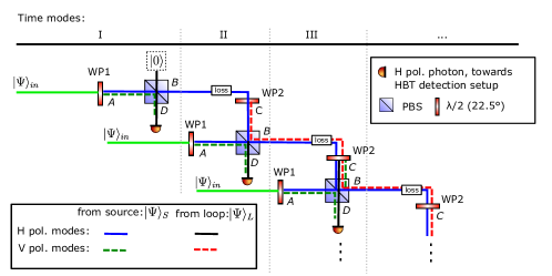
Figure S1: Flow chart of the computer algorithm to calculate $g_{HH}^{(2)}(0)$. It is an unfolded version of the real experiment where photons in mode $D$ are sent to the HBT detection setup, each of these ports corresponds to a different time mode.

In order to model the continuous time-averaged measurements, we have to create a stable photonic field in the initially empty delay loop. In Fig. S2 we show how the average photon number $\overline{n}$ and $g_{HH}^{(2)}(0)$ evolve with the number of round trips. We observe initial fluctuations in both parameters and very good convergence from 20 round trips on, which we use for all calculations in this paper.

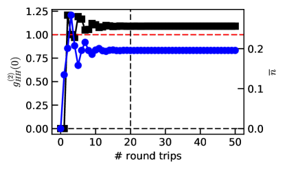
Figure S2: Correlation $g_{HH}^{(2)}(0)$ (black) and average photon number $\overline{n}$ (blue) as a function of the number of round trips for perfectly indistinguishable photons ($M=1$) and experimental round-trip loss $\eta_{L}=0.9$. The vertical line shows our choice of 20 round trips where the field is sufficiently converged.

.2.1 Quantum interference at waveplate WP2 in the delay loop

As explained in the main text, this waveplate leads to quantum interference and Hong-Ou-Mandel photon bunching, not only of two photons but also of higher photon number states. In particular to also model partially distinguishable photons, the effects of WP2 has to be modelled carefully in the computer simulation. We define an $h$-photon Fock state of $H$-polarized photons in spatial mode $S$ by $|0,h\rangle_{S}$ and an $v$-photon Fock state of $V$-polarized photons in the $L$-mode by $|v,0\rangle_{L}$. If the photons are completely distinguishable (wave-function overlap $M=0$), the general WP2 transformation is

$$|0,h\rangle_{S}\otimes|v,0\rangle_{L}\xrightarrow[M=0]{WP2(22.5^{\circ})}\frac{1}{\sqrt{v!}\sqrt{h!}}\left(\frac{1}{\sqrt{2}}\right)^{v+h}\sum_{j=0}^{h}\binom{h}{j}(V_{S}{}^{\dagger})^{j}(H_{S}{}^{\dagger})^{h-j}|0\rangle\otimes\sum_{k=0}^{v}\binom{v}{k}(-V_{L}^{\dagger})^{k}(H_{L}^{\dagger})^{v-k}|0\rangle.$$ (S19)

The photons are individually transformed in 2-dimensional subspaces of Hilbert space and do not interfere.

On the other hand, quantum interference of completely indistinguishable photons ($M=1$ and $\left\{H,V\right\}_{S}=\left\{H,V\right\}_{L}$) will lead to photon bunching:

$$|v,h\rangle_{L}\xrightarrow[M=1]{WP2(22.5^{\circ})}\frac{1}{\sqrt{v!}\sqrt{h!}}\left(\frac{1}{\sqrt{2}}\right)^{v+h}\sum_{k=0}^{v}\sum_{j=0}^{h}\binom{v}{k}\binom{h}{j}\left(-1\right)^{k}(V_{L}^{\dagger})^{k+j}(H_{L}^{\dagger})^{h+v-k-j}|0\rangle.$$ (S20)

In general, WP2 transforms a partially indistinguishable state like

$$\sqrt{M}\cdot|v,h\rangle_{L}+\sqrt{1-M}\cdot|0,h\rangle_{S}\otimes|v,0\rangle_{L}.$$ (S21)

.2.2 Delay loop: Round-trip loss and diffraction

As usual in quantum optics, we model loss in the delay loop by a beamsplitter, before WP2, with transmission $t$ and reflection $r$. Ignoring the empty input port and the dumped output port, this transforms an $n$-photon input state (single polarization) as

$$|n\rangle\xrightarrow[\text{}]{}\frac{1}{\sqrt{n!}}\sum_{k=0}^{n}(ir)^{n-k}t^{k}(a^{\dagger})^{k}|0\rangle.$$ (S22)

Figure S3(a) shows simulation results of $g_{HH}^{(2)}(0)$ for distinguishable and indistinguishable photons, as a function of round-trip loss. Both curves approach single-photon correlations for high loss, which is understandable because in this case the delay loop can be neglected. For low loss, $g_{HH}^{(2)}(0)$ depends strongly on distinguishability, this is why we can use this as a measure of quantum interference.

We do not use relay lenses in the free-space delay loop setup, here we investigate diffraction between round trips. In order to estimate the decrease of mode overlap with the number of round trips, we calculate the propagation-dependent $M$ to be $M(z)=|\frac{kw_{0}^{2}}{kw_{0}^{2}+iz}|^{2}$, where $k$ is the wave number, $z$ the propagation length, and the beam waist $w_{0}=0.50\pm 0.02\mathrm{mm}$. This leads to considerably reduced distinguishability already after 3 round trips as shown in S3(b), however, in combination with the experimental round-trip loss, its effect on $g_{HH}^{(2)}(0)$ is negligible as shown in Fig. S3(a).

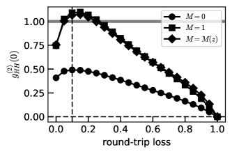
(a)(b)

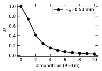
Figure S3: Effects of round-trip loss and diffraction. (a) Dependence of $g_{HH}^{(2)}(0)$ on round-trip loss, for the case of fully distinguishable ($M=0$), indistinguishable ($M=1$) photons, as well as round-trip dependent indistinguishability due to diffraction. The vertical dashed line points to our experimental round trip loss of ~0.1. (b) Effect of gaussian mode diffraction on the distinguishability or wave function overlap $M$.

.3 Visibility measurement

We determine the wave-function overlap $M$ on WP2 by measuring the classical interference visibility $V=\frac{I_{\mathrm{max}}-I_{\mathrm{min}}}{I_{\mathrm{max}}+I_{\mathrm{min}}}$ of laser light sent to the delay loop Ollivier2020_SM , where $I_{\mathrm{max}}$ and $I_{\mathrm{min}}$ are maximal and minimal intensity. The relative phase is changed simply by scanning the laser frequency in this unbalanced interferometer. The change in $V$ corresponds directly to the wave-function overlap $M$ at WP2. We repeat this measurement before and after the long correlation measurements in order to determine errors caused by thermal drift of the delay loop during collecting data, which determines the error bars in Fig. 5 in the main text. Fig. S4 shows examples for visibility measurements with misaligned and aligned delay loop.

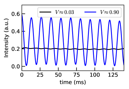
Figure S4: Background-noise corrected interference measurements for misaligned (black) and aligned (blue) delay loop, the obtained visibility $V$ is indicated in the legend.

.4 How many photons do interfere?

A coherent state contains contributions from a large number of different photon number states, a natural question about our artificial coherent states is therefore: What is the highest photon number state that is required to explain our experimental data? Here we explore this by truncating out computer simulation and comparing to experimental data. Figure S5(a) shows simulated $g_{HH}^{(2)}(0)$ for loop transmission $\eta_{L}=0.9$ and ideal alignment with $M=0.9$. This state is now truncated to $n_{\mathrm{max}}$ photons and $g_{HH}^{(2)}(0)$ is calculated, see Fig. S5(a). In Fig. S5(b) we show the predicted $g_{HH}^{(2)}(\tau)$ based on Eq. (4). We clearly see that at least 3 photons are needed to explain our experimental data, but also that discriminating detection of higher number states is impossible with this method because of the differences in $g_{HH}^{(2)}(0)$ become negligible.

(a) (b)

Figure S5: Influence of higher photon number states based on truncated computer simulations. (a) Dependence of $g_{HH}^{(2)}(0)$ on the maximum photon number, the inset shows the full (gray) and truncated (black) simulated photon number distribution ($M=0.9,\eta_{L}=0.9$). (b) Comparison of differently truncated simulations to the experimental $g_{HH}^{(2)}(\tau)$ data. At least 3 photons are needed to explain the experimental data.

This claim is supported by counting simply the number of dips in $g_{HH}^{(2)}(\tau)$ in Fig. 3(b), where clearly dips can be observed at $\tau/R=\pm 1$ (corresponding to two photons), $\tau/R=\pm 2$ (three photons), and less clear for four photons.

Finally, we estimate the rate $R_{n}$ with which $n$-photon states are produced in our setup. We detect single photons with approximately $R=150$ kHz, which corresponds to a single-photon rate entering the HBT setup of approximately $R\cdot 2/\eta_{d}$, where $\eta_{d}$ is the single-photon detection efficiency. From our simulation, we derive the $n$-photon probability $P(n)$, with which we obtain a three-photon rate of $\approx$ 4.8 kHz, a four-photon rate of $\approx$140 Hz and a 5-photon rate of $\approx 1$ Hz.

.5 Properties of the artificial coherent state

In the main text, we showed that the artificial coherent state for $M\approx 1$ approaches the photon number distribution of a weak coherent state and reaches $g^{(2)}(0)\approx 1$. In Fig.S6(a), we compare the same states by means of their Wigner function $W(q,p)$, where $q$ and $p$ are dimensionless conjugate variables corresponding to electric field quadratures. Both, the position and the value of the maximum of $W(q,p)$ show that the artificial states are very close to a coherent state. The presence of negative regions in the Wigner function evidences nonclassicality, connected to the ability to create multi-photon entangled states with a delay-loop setup Istrati2020_SM .

Coherent states have the unique property of being eigenstates of the annihilation operator $\hat{a}$. We test this and show the result in Fig.S6(b), this shows that the artificial coherent states are very close to being an eigenstate of the annihilation operator, it is almost unchanged by several applications of $\hat{a}$. On the other hand, performing the same procedure with a thermal state leads to pronounced changes, where the vacuum-state probability decreases strongly and higher number probabilities are increased.

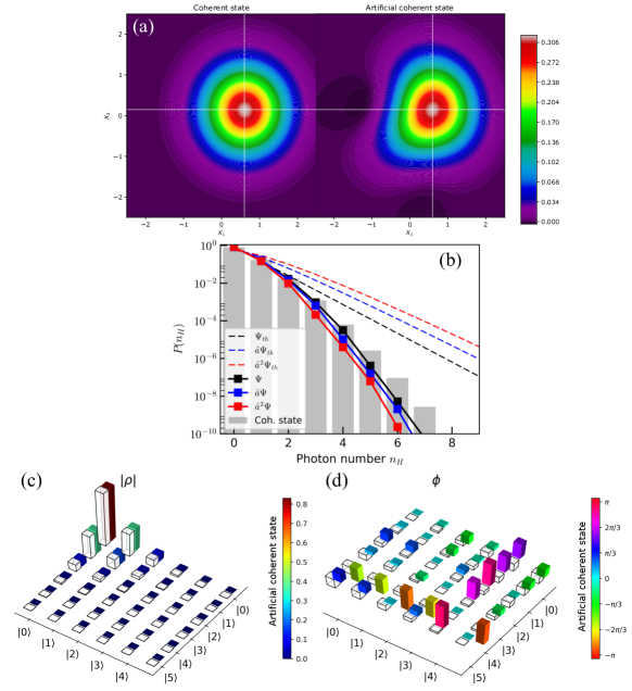
Figure S6: Comparison of our artificial coherent state to a weak coherent state with identical mean photon number ($\bar{n}\approx 0.2)$. (a) False-color plots of the Wigner function $W(q,p)$ of the artificial coherent state (left panel; $M=1,$ round-trip loss 0.1) and of the weak coherent state (right panel). Both $W(q,p)$ share the position of their maximum (intersection of white lines) as expected. (b) Probability distribution after repeated application of the annihilation operator $\hat{a}$ on the artificial coherent state ($\Psi$, squares) and a weak thermal state ($\Psi_{th}$, dashed lines). Bars show the exact coherent state which is an eigenstate of $\hat{a}$. (c) Magnitude and (d) phase of density matrix elements of the coherent (wireframe boxes) and the artificial coherent states (colored bars).

In Fig. S6(c) and (d), we compare the density matrices of the exact weak coherent and artificial coherent states. The similarity in the density matrix magnitude, Fig. S6(c), supports again the closeness of the states; the difference between both states appears mostly in the phase and only for the higher photon number states with low magnitude, see Fig. S6(d).

References

- (1) Kurtsiefer, C., Mayer, S., Zarda, P. & Weinfurter, H. Stable Solid-State Source of Single Photons. Phys. Rev. Lett. 85, 290 (2000).
- (2) Ollivier, H., Thomas, S. E., Wein, S. C., de Buy Wenniger, I. M., Coste, N., Loredo, J. C., Somaschi, N., Harouri, A., Lemaitre, A., Sagnes, I., Lanco, L., Simon, C., Anton, C., Krebs, O. & Senellart, P. Hong-Ou-Mandel Interference with Imperfect Single Photon Sources. Phys. Rev. Lett. 126, 063602 (2021).
- (3) Istrati, D., Pilnyak, Y., Loredo, J. C., Antón, C., Somaschi, N., Hilaire, P., Ollivier, H., Esmann, M., Cohen, L., Vidro, L., Millet, C., Lemaître, A., Sagnes, I., Harouri, A., Lanco, L., Senellart, P. & Eisenberg, H. S. Sequential generation of linear cluster states from a single photon emitter. Nature Communications 11 (2020). eprint 1912.04375.