Imaginarity-free quantum multiparameter estimation
Abstract
Multiparameter quantum estimation is made difficult by the following three obstacles. First, incompatibility among different physical quantities poses a limit on the attainable precision. Second, the ultimate precision is not saturated until you discover the optimal measurement. Third, the optimal measurement may generally depend on the target values of parameters, and thus may be impossible to perform for unknown target states.
We present a method to circumvent these three obstacles. A class of quantum statistical models, which utilizes antiunitary symmetries or, equivalently, real density matrices, offers compatible multiparameter estimations. The symmetries accompany the target-independent optimal measurements for pure-state models. Based on this finding, we propose methods to implement antiunitary symmetries for quantum metrology schemes. We further introduce a function which measures antiunitary asymmetry of quantum statistical models as a potential tool to characterize quantumness of phase transitions.
1 Introduction
Incompatibility residing in simultaneous measurements of different quantities has been a widely acknowledged character of quantum mechanics. Besides the philosophical implications, the measurement incompatibility imposes practical limitations on quantum information processing.
The measurement incompatibility is particularly troubling for quantum metrological tasks which aim at estimating parameters with ever increasing precision [1, 2]. In its early stages, quantum metrology focused on single-parameter estimations. Quantum correlations unlock a region of precision which could never be reached by classical mechanics [3, 4, 5, 6, 7, 8]. The ultimately attainable precision limits are given by quantum Cramér-Rao bounds (QCRBs). [9, 10, 11, 12].
Quantum correlations remain advantageous for various quantum multiparameter metrological schemes [13, 14]. Simultaneous estimations outperform combinations of individual estimations for sensing multi-dimensional fields [15] and imaging [16, 17]. This motivates experimental realizations of multi-parameter metrology [18, 19, 20, 21].
Despite the rapid growth of multiparameter estimation, the status of multiparameter QCRBs [22, 23] has always been under doubt. There are systems which do not allow compatible estimation, rendering QCRBs unattainable [24]. Therefore, conditions to realize compatible multiparameter estimation have been under intense scrutiny [25, 26, 18, 24, 27, 28, 15, 29, 30, 31, 32, 33]. Attainable precision limits for incompatible estimations are also avidly studied [34, 11, 35, 36, 37, 38, 39, 27, 25, 40, 41, 42, 14, 43, 44, 45, 46]. Whether or not the QCRB is saturated, identifying attainable precision limit is the first step of quantum multiparameter metrology.
However, even if one could identify the best precision bound, optimal measurements to attain it can be difficult to perform, and further investigations have been carried out in order to study the implementation of the optimal measurements for given quantum statistical models [25, 16, 47, 29, 48, 30, 39, 49, 50]. Somewhat paradoxically, preceding methods assume knowledge on the target point to be estimated in order to identify the optimal measurement [25, 16, 29, 30], rendering the parameter estimation task to, strictly speaking in the case, applicable only for local parameter estimation.
Yang et. al. [39] presents a method to attain the best precision limit without any prior knowledge of the target point. The method is composed of two steps: a rough expectation of the target-point by a tomography, and the precise estimation with the optimal measurement depending on the rough expectation. The measurement setting has to be adaptively updated according to the previous measurements. Thus the measurement still depends on the target-point.
Another drawback of proposed optimal measurements is the inclusion of projectors onto the target state [16]. Such a projector could be highly entangled for quantum metrology. This is why optimal measurements are sometimes given up in multiparameter quantum metrology [15].
This article proposes the use of antiunitary symmetries to side-step the problems of incompatibility and unfeasible measurement in multiparameter quantum estimation. Any quantum statistical model endowed with an antiunitary symmetry is compatible, which means that the QCRB is attainable in the asymptotic limit. Furthermore, if the system consists only of pure states, the antiunitary symmetry guarantees a target-independent optimal measurement. The construction of globally optimal measurements requires a step beyond the studies of compatibility conditions [25, 28, 15, 29, 30, 33]. Our optimal measurement has a continuous degree of freedom, and one can choose any of them to achieve the global optimality.
With these advantages in mind, we present methods to implement antiunitary symmetries in multiparameter quantum metrology. The so-designed pure-state models for quantum metrology have globally optimal measurements by construction. Our methods do not sacrifice the attainable precisions when implementing antiunitary symmetries.
Though unrecognized, popular models such as N00N states [51, 52, 2], antiparallel spins [53, 54] and 3D magnetometry [15] enjoy antiunitary symmetry. For parameter estimations of these models, we point out how to make the full use of their antiunitary symmetry. For example, we obtain an optimal measurement for the 3D magnetometry which is only bipartite-entangled irrespective to the system size.
Besides practical implications, our result bridges two seemingly different concepts, namely, the incompatibility and the imaginarity. The incompatibility characterizes quantumness of phase transitions in quantum statistical mechanics [55, 56, 57, 58, 59, 43]. The imaginarity is formulated as a meaningful resource in quantum information processing [60, 61, 62]. We refine the relation between these two concepts.
We start by reviewing theories of quantum multi-parameter estimation and antilinear operators in Sec. 2. Section 3 presents the notion of antiunitary symmetry of quantum statistical models, with its direct link to compatible, optimal, and target-independent multiparameter estimations. Then we propose methods to implement antiunitary symmetry in metrological settings in Sec. 4. Section 5 offers discussions concerning a refinement of the link between antiunitary symmetry and compatibility. We offer our conclusion at Sec. 6.
2 Preliminaries
2.1 Quantum multi-parameter estimation theory
Let us consider an estimation of parameters that determines density operators of finite dimensional Hilbert space . The density operator is parametrized by . The set is called a quantum statistical model or simply a model. The task is to estimate parameters from results of quantum measurements performed on multiple copies . The identical measurement on is assumed to be performed independently times. Each measurement on can be entangled over the copies. An estimation process is described by the pair of a positive operator-valued measures (POVMs) and an estimator , where is the set of measurement results ( stands of the space of bounded linear operators).
Precision of estimation is characterized by the following mean square error matrix:
| (1) |
where for . For estimators satisfying
| (2) |
the mean square error matrix is a covariance matrix around the target-point (true value) . We consider locally unbiased estimators and consistent estimators in this article. The estimator is called locally unbiased at when (2) and
| (3) |
holds at the point ( stands for the partial derivative with respect to ). The estimator is called consistent if (2) is satisfied at any point in the asymptotic limit, namely, if
| (4) |
holds (to be more precise, consistency is defined on a sequence of estimators for ). The maximum likelihood estimator
| (5) |
is consistent. While consistent estimators assume sufficiently many rounds of measurements, the unbiasedness condition (4) holds globally over the parameter space .
One of the goals of quantum multiparameter estimation is to find the optimal estimator and measurement to minimize the covariance matrix . Classical and quantum Cramér-Rao bounds deal with the minimization over estimators and measurements, respectively. Define the classical Fisher information matrix (CFIM) for measurement by
| (6) |
where represents the partial derivative with respect to . CFIM provides the classical Cramér-Rao bound of the covariance matrix
| (7) |
At any point , there exists an -dependent locally unbiased estimator saturating the inequality for any (see e.g. Chapter 2 of [63] for an explicit construction of the estimator). Note that the locally unbiased estimator at is generally impossible to construct if the target-point is unknown. The maximum likelihood estimator saturates the same inequality globally in the asymptotic limit .
The remaining optimization is about the measurement. For general model , symmetric logarithmic derivatives (SLDs) () are Hermitian operators defined indirectly by
| (8) |
The solution of Eq. (8) is not unique but one is given by
| (9) |
SLDs define quantum Fisher information matrix (QFIM) via [9, 10]
| (10) |
and provides the quantum Cramér-Rao bound (QCRB) of the CFIM
| (11) |
which holds for any measurement [22, 23]. While SLDs are not necessarily determined uniquely by Eq. (8), the QFIM is independent of the choice of SLDs.
For multiparameter estimation , the QCRB is not necessarily saturated by any measurement, unlike for single-parameter estimations. This limitation is caused by the incompatibility between estimations of different parameters. A necessary and sufficient condition for the saturation in the limit is the weak commutativity [25, 28]:
| (12) |
The matrix is called as the mean Uhlmann curvature [55], and is independent of the choice of SLDs. In this article, compatible models refer to weakly commutative models.
If the saturation occurs for , then the multiple product of the same measurement on the copied model saturates it for any , since the CFIM is additive with respect to the tensor product and separable measurements. For , a necessary condition for the saturation is the partial commutativity:
| (13) |
where is the projector onto the support of [30]. A sufficient condition for the saturation of QCRB with is quasi-classicality represented by
| (14) |
at the point in question. Quasi-classical models do not demand collective measurements for saturating the QCRBs.
All pure weakly commutative models are quasi-classical, and have measurements to saturate QCRB (11) with [25]. For a pure-state model , a necessary and sufficient condition for a POVM on to saturate QCRB (11) at is [30],
| (15) |
and
| (16) |
for any element of . Note that condition (15) should be interpreted so that when the vector on the right-hand-side of the equation is zero, condition (15) still holds with a real infinity [64]. More precisely, condition (15) is equivalent to
| (17) |
While this interpretation of condition (15) is not obvious in the first look at the statement of [30] Theorem 2, it can be deduced from its proof.
As in the case for single-parameter estimation, the optimal measurement generally depend on the target point to be estimated. Explicit methods to construct the optimal measurements proposed so far typically generates parameter-dependent POVMs [16, 30]. To perform such a measurement, one needs a prerequisite knowledge on the point , or must start from adaptive measurements to find in advance.
2.2 Antiunitary operators
We review basic properties of antiunitary operators on finite dimensional Hilbert spaces. Differences between general antiunitary operators and conjugations are relevant in this article. More advanced review on the topic can be found in [65].
An operator on is said to be antilinear if
| (18) |
holds for any complex coefficients and vectors . The Hermitian adjoint of an antilinear operator is defined differently to linear ones by
| (19) |
from which , , and follow for antilinear operators and linear operator . Hermitian adjoints of antilinear operators are again antilinear. Antilinear operator is said to be Hermitian and unitary when and hold, respectively. Unitary antilinear operators are called antiunitaries. Hermitian antiunitary operators are called conjugations. Equivalently, conjugation is an antiunitary satisfying . In this article, antiunitary operators are represented by , and conjugations are by .
A conjugation is a complex conjugation in its reference-bases. To see this, choose a basis of a -dimensional Hilbert space . Define a matrix representation of antilinear operator in this basis by
| (20) |
from which
| (21) |
follows. The matrix is unitary and symmetric when is unitary and Hermitian, respectively. A conjugation has a symmetric unitary matrix representation , and thus decomposed as
| (22) |
with a unitary matrix . This is a direct consequence from AutonneTakagi factorization. Inserting Eq. (22) to Eq. (21), we have
| (23) |
The action of is thus a complex conjugation in the -rotated basis .
The reference-basis of a conjugation is not unique. If a basis is a reference-basis of , then another basis defined by
| (24) |
with a real orthogonal matrix is also a reference-basis of .
A general antiunitary operator has a decomposition
| (25) |
into a (linear) unitary operator and a conjugation . is a conjugation if is symmetric with respect to the reference basis that makes a complex conjugation. Otherwise is an antiunitary that is not a conjugation.
Spin-flip is an example of antiunitary operator that is not a conjugation. Consider a 2-dimensional space with a basis . Spin-flip is defined by
| (26) |
where is the Pauli- operator and is the complex conjugation in the same basis. Obviously is not symmetric, and .
In most part of this article antiunitary operators act in adjunction
| (27) |
on (linear) Hermitian operators such as quantum states. The above operator is equal to
| (28) |
from Eq. (25), where is the complex conjugation of in the reference basis of . The adjoint action of conjugation on a Hermitian operator is equivalent to transposition since . When is a quantum state, namely, a density operator, the transformation cannot be a completely positive map.
Direct sums and tensor products of antiunitary operators are well-defined, and both result in antiunitary operators again. The tensor product of antiunitary operators on and on is defined By
| (29) |
for vector in the composite system . For arbitrary two vectors in decomposed by
| (30) | ||||
| (31) |
the inner product is calculated as
| (32) |
by using Eq. (29). Equation reveals that is well-defined and is antiunitary. We also have
| (33) |
where and are linear operators, and the tensor product in the middle is of linear operators. Tensor products of pairs of an antiunitary operator and a linear operator is not well-defined. There is no “partial conjugation,” in contrast to the well-defined partial transposition.
3 Global antiunitary symmetry
This section presents a direct link between antiunitary symmetry and weak commutativity. Theorem 2 states that quantum statistical models with “global” antiunitary symmetries are weakly commutative at all points in the parameter spaces. Theorem 3 ensures the target-independent optimal measurements for pure-state models with global antiunitary symmetries. These theorems underlie our methods to find globally optimal measurements.
3.1 Global antiunitary symmetry and conjugation
Let us define models with global antiunitary symmetry, and clarify the distinction between general antiunitaries and conjugations with respect to the definition.
Definition 1
A quantum statistical model is said to have a global antiunitary symmetry (GAS) when there is an antiunitary operator such that
| (34) |
holds for any . Models with GASs are said to be imaginarity-free.
The antiunitary operator in the definition does not depend on the parameter . This is why we call the antiunitary symmetry in the sense of Def. 1 as being global.
As a trivial example, any classical model, whose states are diagonal in a fixed basis for all , i.e., when all the eigenvectors are independent of , is imaginarity-free. The antiunitary operator is the complex conjugation in the diagonal basis.
There also are various non-classical imaginarity-free models. This article presents GASs of N00N states [51, 52, 2], super-dense coding [66] and 3D magnetometry [15] in Sec. 3.4, and of antiparallel spins [53, 54], qubit inside a disc of Bloch sphere [27] and embedding quantum simulators [67, 68, 69, 70, 71, 72] in Appx. A.
The GAS must be a conjugation for certain classes of models.
Lemma 1
A GAS, if exists, is given only by a conjugations if the model satisfies either of the following two conditions:
(a) is a pure state at all points in and the pure states span the entire Hilbert space ,
(b) is non-degenerate at some point in .
We use following two lemmas to prove lemma 1.
Lemma 2
For any antiunitary operator and a vector on a Hilbert space , implies .
proof) holds if and only if with some unimodular . This implies .
Lemma 3
Let be an Hermitian operator on Hilbert space with eigensubspaces (), and be an antiunitary operator on which satisfies . Then has a decomposition
| (35) |
where is an antiunitary operator on for each .
proof) Let us denote the eigenvector of with eigenvalue by . Then we have
| (36) |
for any eigenvalues , where the second equality follows from .
Equation (36) is possible only if when , and are orthogonal to each other.
Equivalently, implies .
Thus is a sum of antiunitaries on the eigensubspaces of .
proof of lemma 1)
(a) Let be the GAS of a pure state model .
We have at all points from Lem. 2.
Because is linear and is spanned by , must be identity.
(b) Let be the point where becomes non-degenerate.
As is Hermitian and satisfies , lemma 3 reveals a decomposition of given by Eq. (35).
The dimension of eigensubspaces are all because of the non-degeneracy.
Then lemma 2 applies to each , and we have .
This implies , and completes the proof for the case (b).
Even if a model has a GAS which is not a conjugation, the same model has another symmetry provided by a conjugation:
Theorem 1
If a model is imaginarity-free, there is a conjugation which is a GAS for .
This theorem remains valid even if the model is replaced by any set of Hermitian operators, where the definition of GAS is straightforwardly extended.
In the proof presented below, can be a Hermitian operator and can be a discrete set.
proof)
Let be a set of Hermitian operators in Hilbert space with a GAS .
We explicitly construct a conjugation replacing .
Let be the disjoint subspaces of that are simultaneous eigensubspaces of all the states in . The state is decomposed as
| (37) |
where are projectors each onto , is a projector onto the complement subspace
| (38) |
and are eigenvalues.
For arbitrary vector orthogonal to , there is a point such that is in the complement subspace of the eigensubspace of with eigenvalue . By applying Lem. 3 to , we obtain a decomposition of such that belongs to the different sector from . As is any vector orthogonal to , we have a decomposition of the antiunitary
| (39) |
where antiunitary operators and acts on and its complement, respectively. Since the decomposition (39) exists for each , we have
| (40) |
where is an antiunitary operator on .
The defining equation of the GAS is rewritten by the decompositions of the state (37) and the antiunitary (40) to
| (41) |
for the truncated (unnormalized) state , and
| (42) |
Any antiunitary operator on satisfies Eq. (42) instead of . Thus all in can be replaced by conjugations.
We now show that is a conjugation. To do this, we consider the following step-by-step procedure to decompose and . The procedure starts from with the trivial decomposition and , and ends at with a decomposition of into -dimensional subspaces.
At the step , a disjoint subspace decomposition () of and corresponding decomposition of antiunitary is given. Choose a subspace with dimension more than , say , and a unit vector therein. By definition of the truncated state , there is a point such that is not an eigenvector of . From Lem. 3, is decomposed as
| (43) |
where and are antiunitary operator on disjoint subspaces , (), respectively, such that is not orthogonal to either or . For the two decompositions (43) and to be consistent, we necessarily have the subspace decomposition () of defined by
| (44) | ||||
| (45) | ||||
| (46) |
and the corresponding decomposition of antiunitary.
At the end of the procedure, we obtain the decomposition of antiunitary
| (47) |
into -dimensional antiunitaries. Since any -dimensional antiunitary must be a conjugation, is a conjugation for all , and hence is, too.
Now that is a conjugation and can be replaced by a conjugation on for all ,
| (48) |
is a conjugation on which satisfies Eqs. (41) and (42).
Thus is a conjugation that gives the GAS for .
When a conjugation provides a GAS for model , there is a basis that represents as a real matrix for all . The model is “free from imaginarity” in this sense. Conversely, any model consisting only of real density matrices have a conjugation as a GAS. Theorem 1, by identifying antiunitary-symmetric models with conjugation-symmetric models, justifies the term “imaginarity-free” to be used on models with GASs.
3.1.1 Antiunitary symmetry defined on horizontal lift
A lift of a quantum statistical model is its orbit in the associated fiber bundle. For pure-state models, the defined GAS is equivalent to the antiunitary symmetry on the so-called horizontal lift of the model. We briefly explain this equivalence without any prerequisite knowledge on geometry here. The content of this section is independent on other parts of this article. See [73, 74] for complete expositions.
For a pure-state model , a lift is identified with a parameterized unit vector in such that
| (49) |
for any . The lift is said to be horizontal, if it satisfies
| (50) |
for any and . The horizontal lift exists if and only if the model is quasi-classical.
The global antiunitary symmetry (GAS) of a horizontal lift is defined as the antiunitary operator such that
| (51) |
holds for any . Now it is readily seen that becomes a GAS of the model . Conversely, if a model has a GAS , then there is a lift satisfying (51). This lift is horizontal since and are in the same real subspace of invariant by the antiunitary .
The model has a GAS if its horizontal lift does, and they share the same antiunitary operator.
3.2 Global antiunitary symmetry and weak commutativity
The weak commutativity is ensured by a GAS.
Lemma 4
If model has a GAS , there is an SLD satisfying for any point and for any parameter .
Theorem 2
Any imaginarity-free model is weakly commutative at any point in .
proof) Let be the GAS of model . From Lem. 4, there are SLDs satisfying for all . For these SLDs we have
| (53) |
Therefore the Uhlmann curvature (12) is zero for any pairs of .
According to Thm. 2, parameter encoding schemes are not crucial for compatible multiparameter estimations. There are physical systems which provide only weakly commutative models, irrespective to the parameter encoding schemes. For example, Majorana fermions have antiunitary particle-hole symmetry. Thus any models constituting of Majorana fermions are weakly commutative.
Quantum mechanics in real Hilbert spaces lacks an uncertainty principle between observables of a specific form [75]. If and are observables such that and , the expectation value is zero for any real density operator . The Heisenberg uncertainty principle is trivialized. Nevertheless there is an uncertainty principles of a different form [75, 76].
We are not sure how Thm. 2 relates to the absence of Heisenberg uncertainty principle. The link between uncertainty principles and incompatibility of parameters should be clarified in more detail. Such an attempt has started only recently [77].
Theorem 2 directly relates geometric phases and the phases of off-diagonal elements in density operators. The mean Uhlmann curvature is the Uhlmann geometric phase (per unit area) accumulated by infinitesimal loops around the point [55]. The Uhlmann geometric phase coincides to Berry phase for pure states [78]. If the phases of off-diagonal elements of the density operator are all zero at the neighborhood of , the geometric phases accumulated by infinitesimal loops around the point is also zero.
Antiunitary symmetries are sometimes easier to check than the zero of mean Uhlmann curvature. Consider thermal state of a parametrized Hamiltonian presented by a canonical ensemble . Here we assume that the temperature is contained in the Hamiltonian as a parameter. Such a model is rather studied in quantum statistical mechanics, than in quantum metrology. Non-zero mean Uhlmann curvature characterizes quantum phase transitions of the thermal state [55, 56, 57, 58, 59, 43]. Lemma 3 indicates that is imaginarity-free if and only if does. That is, if the Hamiltonian endows with an antiunitary symmetry such as time-reverse, the thermal state has zero mean Uhlmann curvature.
One might wonder if QFIMs of imaginarity-free models have a particular form. As we will see in Sec. 4.2, it is possible to construct an imaginarity-free model with QFIM from arbitrary model with QFIM . GASs do not pose any restriction on the form of QFIMs. As a consequence, imaginarity-freeness does not imply the stricter notion of “compatibility” referring to the saturation of QCRBs with diagonal QFIMs [28].
As a final remark, there are weakly commutative models without any GAS. This implies that the converse of Thm. 2 is not true in general: weak commutativity does not necessarily imply imaginarity-freeness. Even some single-parameter models, such as off-equator phase estimation presented in Appx. A.1.2, do not have any GAS.
3.3 Optimal target-independent measurements
Any imaginarity-free pure-state model is accompanied by a set of globally optimal POVMs. This means that the QCRB is saturated by the corresponding measurement at any target-point.
In this section, we set the number of copies in joint measurements to , because we focus mainly on pure imaginarity-free models which are automatically quasi-classical [25].
A set of optimal POVMs is known for antiparallel spins [54] (see Appx. A.1.3 for details). These POVM operators are first proposed in [53], and proven to maximize a fidelity measure [79]. The POVMs must be independent from the target point in the parameter space, in order to be optimal for the fidelity measure. Later the same set of operators is shown to saturate QCRB [54], namely, it is optimal in terms of a precision bound as well.
The target-independent POVMs are fascinating because they are optimal all over the parameter space. In general, around different regions in the parameter space, we require different POVMs to achieve the best precision limit in the region. This is the case even for single-parameter estimations. If the optimal POVMs are independent of the target point, the precise measurement can be carried out without any prerequisite knowledge on the source.
The following theorem presents target-independent optimal POVMs.
Theorem 3
Let be an antiunitary on . Any POVM satisfying conditions
| (54) | ||||
| (55) |
saturates the QCRB (11) of a pure-state model with everywhere in if is a GAS of .
Since CFIM is additive with respect to tensor products and product measurements, the product of antiunitary-invariant rank-1 measurements saturates the QCRB (11) for any .
For proving Thm. 3, we use the following lemma to restrict GASs to conjugations. Recall that any imaginarity-free model has a conjugation as a GAS (Thm. 1).
proof) If is a conjugation, projectors onto vectors of ’s reference-basis form a POVM with required properties.
Conversely, let () be a POVM satisfying conditions (54) and (55).
From Lem. 2, we have for all .
Because spans the entire Hilbert space , we have .
In other words, is a conjugation.
proof of Thm. 3)
From Lem. 5, we can assume that the antiunitary operator is a conjugation .
Let be a POVM satisfying conditions (54) and (55). From Lem. 4, there are SLDs obeying the antiunitary symmetry . It suffices to show that conditions (16) and (17) (Theorems 1 and 2 of [30]) hold for these antiunitary-invariant SLDs and for any element in .
For this purpose, we choose a particular pure-state vector for . Let be the continuously parametrized unit vector such that and hold everywhere. Equivalently, is defined to be the horizontal lift of .
Let be an element of POVM . Take a reference-basis of so that
| (56) |
for , where is a positive coefficient. SLDs are represented by real matrices
| (57) |
in the basis , where are real coefficients. Since spans the real Hilbert subspace of invariant under , the vector of the horizontal lift have the decomposition
| (58) |
with real coefficients .
Now we check the conditions (16) and (17) on . Equation (58) alone implies
| (59) |
and Eqs. (57) and (58) together imply
| (60) |
We find that and are all proportional to by real coefficients. This implies that satisfies conditions (16) and (17) at any point .
Because is an arbitrary element in , conditions (16) and (17) are satisfied by all elements in everywhere.
The optimality of antiunitary-invariant POVM is independent not only on the target point, but also on how the parameters are encoded in the state. The optimal POVMs depend only on the GAS, which in turn depends only on the states as a set. Thus re-parametrization change neither the GAS nor the optimal POVMs. One does not have to use different POVMs according to different parametrization.
The condition on POVMs indicated by Thm. 3 is so loose that continuously many such POVMs exist. To see this, let us consider a pure-state model whose GAS is a conjugation . The conjugation defines a -dimensional real Hilbert subspace of spanned by vectors satisfying . You can take any vectors from this -invariant real subspace to construct the optimal POVM by . For example, the reference basis for representing a conjugation as a complex conjugation is not unique. In Appx. A.1.3, we find two different sets of optimal POVMs for antiparallel spins from its GAS. One of them is given in [53] and the other one is new. As another example, rank-1 projectors distributed randomly over the real subspace also saturates the QCRB [74].
While any antiunitary-invariant measurements work equally well, there should be experimentally preferable ones, such as those requiring less entanglement. Consider, for example, an estimation of parameters encoded as a unitary evolution . A typical method of quantum metrology utilizes multiple copies of the same system driven by . If the -particle Hamiltonian has an antiunitary skew-symmetry , the overall Hamiltonian has an antiunitary skew-symmetry under . We show in Sec. 4.1 how to construct imaginarity-free models based on Hamiltonians’ antiunitary skew-symmetries. If you construct an imaginarity-free model based on the GAS , the POVM must be invariant under . You would prefer the measurement in the product POVM, each being invariant under .
We apply the above reasoning to find the optimal measurement basis for 3D magnetometry [15] in Sec. 3.4.3. There the GAS provides a parameter-independent optimal measurement basis. The entanglement required for the measurement is reduced from -partite to -partite. The search of reasonable measurements is possible thanks to the freedom of the optimal measurement for imaginarity-free models.
We close this section by extending the globally optimal POVMs to globally optimal estimation strategies. Even if a target-independent measurement saturates the QCRB everywhere, the optimal locally unbiased estimator could still depend on the target-point.
Maximum likelihood estimators are independent on the target-point to be estimated. The only condition for the maximum likelihood estimator to work globally is the identifiability of the parameter. More precisely, the probability distribution generated by the measurement must be in one-to-one correspondence with the point . Projectors onto a single reference-basis for will not produce sufficiently informatic probability distributions to identify the parameters in general.
Fortunately, the condition on the optimal POVMs described in Thm. 3 is loose enough to admit the POVMs to identify the parameters. Under the restrictions (54) and (55), it is possible to construct a POVM such that the map from -invariant density operators to is one-to-one. An example of such real-informationally-complete POVMs associated to is the rank-1 projectors distributed randomly over the real subspace defined by [74]. Because the space of real density operators associated to contains if is its GAS, the probability distribution generated by identifies the parameter. In this way we obtain the following corollary:
Corollary 1
Let be an imaginarity-free pure-state model. Suppose that the model is identifiable in that the map is invertible. Then there is a POVM on with which the maximum likelihood estimator satisfies
| (61) |
at any point .
We can globally saturate QCRB by a fixed measurement and a maximum likelihood estimator without any prior knowledge on the target-point, if the pure-state model has a GAS. In practice, there is no need to stick to the real-informationally-complete POVMs. One can employ POVMs that identify the state from the model only.
3.4 Examples of imaginarity-free models
In this section, we introduce three examples of imaginarity-free models. These are N00N states (Sec. 3.4.1), super-dense coding (Sec. 3.4.2), 3D magnetometry (Sec. 3.4.3). The Venn diagram in FIG. 1 summarizes known classifications of weakly commutative models together with imaginarity-free models.
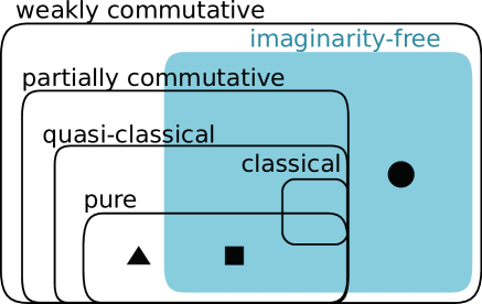
The examples presented in this section all correspond to the square symbol in FIG. 1. To ensure the existences of models at each region of the diagram, we present some other examples in Appendix A.
In this section again, we set the number of copies in joint measurements to .
3.4.1 N00N states
The first example is a single-parameter model. The N00N state of optical interferometry is a milestone of quantum metrology and is still under theoretical and experimental studies. See, e.g. [51, 52, 2] for theoretical reviews and [80] for a review including experiments.
The pure-state model with a phase parameter is given by
| (62) |
where represents a two-mode state having and photons in mode 1 and mode 2, respectively. We can readily see that the N00N state distributes on the equator of Bloch sphere with poles and , and thus can be represented by real density matrices in a suitable basis. Any antiunitary operator satisfying
| (63) | ||||
is a GAS for N00N state model (62). From the GAS (63) we recover a target-independent optimal measurement basis including vectors
| (64) |
The measurement on this basis is carried out by a combination of a beam-splitter and a photon-number-counting measurement.
Note that not all the pure-state single-parameter models are imaginarity-free in general. A counterexample is provided in Appx. A.1.2 by an off-equator phase estimation of a spin. Even for single-parameter models, the globally optimal measurement is not guaranteed if the model does not have a GAS.
3.4.2 Super-dense coding
Fujiwara [66] considered an estimation of SU unitary represented on -dimensional space. The model is given by
| (65) |
where is a -qubit state. The unitary is represented by -parameters. We consider pure input state defined by with a constant . This is a parameter estimation version of super-dense coding [81]. The model is weakly commutative if and only if , namely, when is maximally entangled [66].
Model is indeed imaginarity-free for maximally entangled . For conjugation in the reference basis we have
| (66) | ||||
| (67) |
where we have used identities and holding for any SU unitary . Thus the model is symmetric under the product conjugation followed by .
With the aid of GAS we can construct the target-independent optimal measurement with which is not addressed in [66]. Since Eq. (67) holds for (, represents the Pauli- operator), projectors onto the Bell measurement basis forms a rank-1 antiunitary-invariant optimal POVM. The measurement used by the receiver of original super-dense coding scheme [81] is an optimal measurement for the parameter-estimation version.
If the input state is not maximally entangled, namely, if , there is no unitary on such that holds. Therefore it is impossible to transform Eq. (66) to Eq. (67) by replacing to . Indeed, there is no GAS when because the model (65) is not weakly commutative for these [66].
Note that we did not require the explicit expression of parametrized unitaries to find a GAS. Theorem 2 enables the shortcut in deducing weak commutativity.
3.4.3 3D magnetometry
3D magnetometry has an spin system interacting with the external magnetic field [15]. The Hamiltonian is
| (68) |
where is proportional to the magnetic field, and is the vector of Pauli matrices for th spin. The parameter to be estimated is . The -spin system undergoes unitary transformation . The model of 3D magnetometry is
| (69) |
where is the initial state to be optimized.
Inspired by the single-parameter phase estimation, in [15] they considered
| (70) |
as the initial state. Here is the normalization factor, are constants to be chosen for making the model weakly commutative. State is a -partite GHZ state with eigenstates of Pauli operators . For later convenience, we choose the phases of to have
| (75) | ||||
| (80) | ||||
| (85) |
We consider the symmetry under spin-flip on systems,
| (86) |
where and ’s reference basis is . Since the spin-flip changes the sign of Pauli operators , the unitary evolution is invariant under spin-flip. Thus the spin-flip is a GAS of the model if the initial state is also invariant under the spin-flip.
Now we derive the values of and to make the model imaginarity-free. From our choice of follow
| (87) | ||||
and hence
| (90) |
for any integer . Therefore is the case when and for , and and for with some integer . The model has a GAS and thus is weakly commutative for these and . We are not sure if the difference between our solutions on with those found in [15] is entirely due to the choice of phases since vectors are not explicitly indicated in [15].
Baumgratz and Datta [15] found an optimal measurement basis including the target state , which is -partite entangled. They also considered projectors
| (91) |
and numerically exhibited that these POVMs are close to the optimal. The projector is invariant under the GAS (86) since
| (92) |
holds for all and even . That the high-rank projectors almost achieves the ultimate precision limit is still non-trivial.
We derive different measurement bases which are guaranteed to be optimal from the GAS. The GAS is a tensor product of conjugations . Equation (87) implies that for , the basis
| (93) |
is a reference basis for the bipartite conjugation , and thus has the -product of (93) as a reference basis. This implies that the bipartite measurements in the basis (93), performed independently on copies, is optimal.
4 Methods to implement global antiunitary symmetries
In this section we consider methods to construct imaginarity-free models. The benefit of implementing the GASs is twofold. First, the weak commutativity of the model is ensured at any point (Thm. 2). Second, the models have parameter-independent optimal POVMs (Thm. 3 and Cor. 1), when the models are pure.
We focus on quantum metrology, and thus assume some ability to modify the physical systems to adjust the models. If the model cannot be adjusted, the attainable precision does not improve even if we implement antiunitary symmetry on by pre-measurement operations. The assumed ability is to replace the initial states before interactions.
Even if you can adjust the models, you may still wonder if the restriction to GASs is worth taking. GASs inevitably restrict available models. There may be a model without GAS but still offers better precisions for all the parameters. In short, you may wonder if compatible models offer maximum precisions. Unfortunately, previous methods to design compatible models for quantum metrology did not consider optimizations on the attainable precision [25, 28, 33].
This question has almost been ignored since it was difficult to calculate the optimal precision bounds for incompatible models. To propose a metrology scheme, you have to evaluate the precisions attained by the scheme. If the model is compatible, it suffices to calculate the QCRB. Otherwise you have to calculate the so-called Holevo Cramér-Rao bound [34, 11, 35, 36, 37, 38, 39], whose closed-form expression is missing. This has been one of the reasons for researchers to seek for compatible models. However, methods to calculate the Holevo Cramér-Rao bound has been developed [27, 25, 40, 41, 42, 44], and a semi-definite programming is available now [14]. The complexity is further reduced when you require only a lower bound of the Holevo Cramér-Rao bound [45]. The final blow on the QCRB is its modest advantage: the Holevo Cramér-Rao bound secures at least half of the QCRB even in the worst case [43]. This encourages the pursuit for better precisions in the realm of incompatible models.
Our answer to the question on the simultaneous realizability of best precisions and GASs is twofold.
In Sec. 4.1, we consider a particular generator of unitary transformation. The optimal initial state for the phase estimation inevitably leads to imaginarity-free models. The GAS coexists with the optimal initial state, and provides optimal global measurements at the same time.
In Sec. 4.2, we propose a different method to implement antiunitary symmetry by generalizing antiparallel spins. The method implements GASs without deteriorating the precision limit of a given model, under some symmetry conditions.
4.1 Antiunitary skew-symmetric Hamiltonians
The first method is inspired by 3D magnetometry. Consider a model whose state given by
| (94) |
where is a parametrized Hamiltonian. The Hamiltonian is assumed to have a skew-symmetry
| (95) |
under an antiunitary . If there is a state satisfying
| (96) |
with some unimodular , becomes a GAS of the model (94) by setting the initial state to . The existence of antiunitary skew-symmetry (95) is the key for implementing the GAS.
Now we question the optimality of the antiunitary-invariant initial state (96) for estimating . The N00N state reviewed in Sec. 3.4.1 is antiunitary-invariant and, at the same time, the best initial state for the phase estimation on interferometry. We show in the following that the simultaneous realization of the optimal initial state and the GAS is not a mere coincidence.
Optimal initial states are known for particular single-parameter estimations. Consider a quantum system driven by a traceless generator . Now we are given a task to estimate the single parameter from the state
| (97) |
where the initial state is of our choice. The best initial state that maximizes the quantum Fisher information for of the state (97) is given by [82]
| (98) |
where is arbitrary, and and are eigenstates of with maximum and minimum eigenvalues and , respectively. The optimal state maximizes the quantum Fisher information by maximizing the uncertainty in expecting [83, 84].
We can readily see that the resulting model
| (99) |
is imaginarity-free. The state lies on a great circle of the Bloch sphere of the qubit system spanned by and . Therefore the state is represented with real coefficients in a suitable basis.
When the Hamiltonian has a specific form, a GAS of the model (99) is derived from the antiunitary skew-symmetry of the Hamiltonian. Suppose that the spectrum of the generator distributes symmetrically about the origin. We further assume that the eigensubspaces and belonging to eigenvalues and , respectively, have the same dimension. Then an operator on defined by
| (100) | |||
is an antiunitary. This antiunitary is a symmetry of the initial state. We have and hence
| (101) |
by definition. Moreover, the skew-symmetry
| (102) |
of the generator under the action of follows from the definition.
Combining Eqs. (101) and (102), we arrive at the equality
| (103) |
meaning that is a GAS of the model (97) for any optimal initial state. Its optimal global measurements are lead by Thm. 3 and Cor. 1.
The optimization of initial state presented above underlies single-parameter metrology schemes including the N00N state reviewed in Sec. 3.4.1.
In summary, if the spectrum and the eigensubspaces of generator distribute symmetrically about the origin, the model (97) with any optimal initial state (98) is imaginarity-free. The resulting model with optimal initial state provides the target-independent optimal measurement to attain the best QCRB. For a special generator of this kind, the optimization of initial state naturally leads to imaginarity-free models.
This observation dispels a doubt that GASs spoil advantages of quantum statistical models. Imaginarity-free models look close to classical ones in that the freedom of imaginary numbers disappears, that all the parameters are compatible, and that global optimal measurements exist. The classical behavior can, however, coexist with the most effective metrological schemes offered by quantum models. In this sense, the imaginarity-free estimations benefits from both of classical and quantum estimations.
4.2 Antiparallel model
Our second method requires the state of the original model and its conjugation . This is a non-trivial requirement on the physical system since there is no completely-positive map to transform given state to its conjugation . We consider how to produce mutually conjugate state pairs later. See FIG. 2 for a schematic representation of our second proposal.
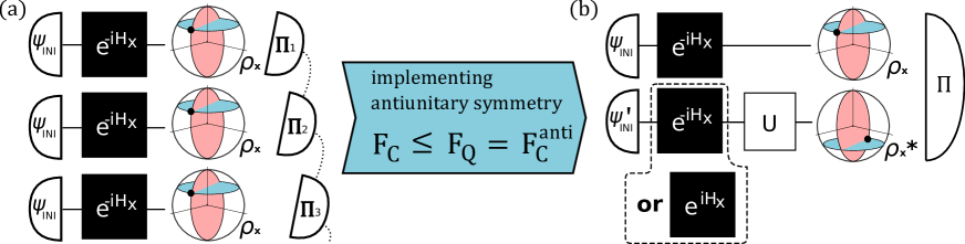
We propose to use, if possible, half-conjugated copies instead of the normal copies .
Definition 2
Let be a quantum statistical model. Antiparallel model for is defined by
| (104) |
where represents a complex conjugation in a fixed basis.
The antiparallel model has a GAS
| (105) |
independently to the original model , where represents the swap operator . Thus the antiparallel model is weakly commutative at any point in the parameter space (Thm. 2) independently to the original model .
The antiparallel model does not deteriorate the attainable precision. QFIMs of the original model (), of the antiparallel model (104) (), and of “parallel model” () are related by
| (106) |
at any point . The second equality is obtained directly from SLDs for the antiparallel model
| (107) |
where are SLDs of the original model. Since the antiparallel model is weakly commutative, the QCRB (106) is asymptotically () attainable on the antiparallel model. The same bound is not attainable on the original incompatible model and the parallel model.
A reference basis to represent the GAS (105) as a complex conjugation is
| (108) |
where are the product basis for the complex conjugation. When the model is pure, the corresponding projectors form an optimal set of POVMs to achieve QCRB (106) with independently to the original model (Thm. 3).
A notable theoretical aspect of “antiparallelization” is its model-independence. According to the precision bound (106), antiparallel state pair always surpasses the parallel one with respect to the attainable precision limit. Mutually conjugated state pairs have revealed their intrinsic utility both theoretically [53, 79, 85, 86, 87, 88, 54] and experimentally [89]. Since these works all focus on restricted models such as spins, the extendible advantages of mutually conjugated state pairs has been kept unknown. The reduction of incompatibility manifests a model-independent benefit of conjugate state pairs.
A potential intuitive reason why the conjugated state pair offers better mean square errors than the mere pair is that the former distributes over larger operator-space compared to the latter. Volumes of spin ensembles characterized by entropy or code dimension are considered to be positively correlated to the fidelity in estimating the direction of spins from the sources of ensembles [53, 90, 91, 88]. We can define a state ensemble from a quantum statistical model, by, for example, assuming uniform distribution over the parameter space. Note, however, that mean square errors are defined locally at each point unlike the ensemble volumes and the fidelity. Therefore mean square error should be compared to certain local quantity such as rate of volume growth around each point, rather than to the ensemble volume itself. We leave the investigation on the ensemble volume of general antiparallel models as a future work.
Note that the antiparallel model is not the only method to implement a GAS independently of the original model. Appendix A.3 introduces a different kind of compatible models which are inspired by embedding quantum simulators [67, 68, 69, 70, 71, 72].
There are instances where the mutually conjugate states and are available at the same time. Here we consider quantum metrological schemes to estimate parameters encoded in a Hamiltonian . Tasks of quantum metrology abstract to estimations of parameters from states with the initial state of your choice. The antiparallel models additionally require the conjugated states . If it is possible to produce arbitrary initial states, the remaining task is to realize conjugate state evolution .
In the following subsections we introduce two major instances where the conjugate state evolution is available.
4.2.1 Hamiltonians’ skew-symmetry
Let us assume that a Hamiltonian flips its sign
| (109) |
under an antiunitary . In this case, the conjugated state evolution can be decomposed to
| (110) |
Namely, the conjugate state evolution is unitarily equivalent to the original evolution . Since the original evolution is available, the conjugated state
| (111) |
can be produced by implementing unitary transformations and before and after the evolution.
4.2.2 Inverse transformation
Suppose that the inverse transformation is available in addition to . Let be any conjugation that leaves invariant. For example, one may take the eigenbasis of as the reference basis for conjugation. Then for any initial state ,
| (112) |
is the conjugate state of .
5 Discussions
5.1 Antiunitary invariant POVMs on mixed states
The antiunitary-invariant POVMs do not necessarily saturate QCRBs for mixed models. This is partly because multipartite measurements () are necessary for saturating QCRBs in general. Any single-copy measurement cannot saturate the QCRB for such a model. Theorem 3 does not generalizes to models with mixed states.
Now you may wonder what if the imaginarity-free mixed-state model is quasi-classical. Any quasi-classical model is accompanied by a (potentially target-dependent) single-copy measurement to saturate the QCRB. Does our antiunitary-invariant POVM saturate QCRBs for quasi-classical mixed models?
The answer is “no.” Even if a quasi-classical mixed state model has a GAS, the antiunitary-invariant POVM does not necessarily form the optimal POVM. A counterexample is given in Appx. A.1.4 by the off-equator estimation on depolarized antiparallel spins. Our antiunitary-invariant POVM is not optimal to this quasi-classical mixed model.
The antiunitary-invariant POVMs do not seem to have any special property in the mixed state regime. In Appx. A.1.4, we demonstrate that different antiunitary-invariant POVMs give different CFIMs for the off-equator phase estimation on depolarized antiparallel spins. This implies that the antiunitary-invariant POVMs do not share anything in terms of the measurement precisions at the mixed state regime. Their coincidence is only at the pure state limit.
5.2 Local antiunitary symmetry
We have seen that the converse of Thm. 2 is not true. There are weakly commutative models without any GAS. To refine Thm. 2, we compare weak commutativity and antiunitary symmetry at each point in the parameter spaces.
We are motivated from the following geometric perspective. Consider application of Thm. 2 to subspaces of the whole parameter space. If is a subspace of the parameter space and if there is a GAS inside , then the model is weakly commutative at all points in . If there are such “small” GASs for covering subspaces , then the model is weakly commutative at all points in . Note that s do not necessarily coincide.
Now a question is, whether any weakly commutative models have such covering subspaces endowed with antiunitary symmetries. While global weak commutativity does not imply GAS, it may imply patchworks of the small antiunitary symmetries. If so, weak commutativity and the existence of antiunitary symmetries should be equivalent at sufficiently small regions. In the light of Thm. 3, such a “local” antiunitary symmetry might be useful for constructing target-dependent optimal POVMs.
The answer to the question is positive for pure-state models and negative in general. We show that all weakly commutative pure-state models have local antiunitary symmetries. However, this result does not extend to mixed-state models. The weakly commutativity does not imply local antiunitary symmetries.
We define the local antiunitary symmetry (LAS) as a straightforward limitation of the GAS to neighborhoods of a point.
Definition 3
A model is said to have a LAS at , if there is an antiunitary operator such that and hold for all .
To see how LAS relates to the GAS, consider the first-order approximation of state around the point :
| (113) |
where are small real numbers. Then the LAS satisfies
| (114) |
in the first-order approximation. Thus if there is a LAS at , the states in a small neighborhood around share an approximately good GAS.
LAS does imply weak commutativity at each point. Furthermore, these two are equivalent for pure-state models.
Theorem 4
If a model has a LAS at , it is weakly commutative at . Pure models have LASs at points where the models are weakly commutative.
The proof of Thm. 4 is delegated to Appx. B.1. The off-equator phase estimation on spin, for example, have LASs at all points, despite having no GAS. This implies that the piecewise antiunitary symmetries do not necessarily joint together to form a single antiunitary symmetry.
The LAS accompanies the optimal POVMs to saturate QCRB for pure-state models (see Appx. B.2 for details). Similarly to the case of GAS (Thm. 3), they are the rank- POVM invariant under the LAS. Since the LAS may depend on the target point, the optimal POVMs are also target-dependent in general.
Regarding mixed states, there are weakly commutative models without any LAS. We can further say that there are quasi-classical models without any LAS when , but not when . Examples are presented in Appx. B.3. The structure of compatibility is more involved than to be explained by antiunitary symmetries.
5.3 Quantifying antiunitary asymmetry
In this section, we try quantifying antiunitary asymmetry of quantum statistical models. Theorems 2 and 4 both states that incompatibility, a unique property of quantum mechanics, is absent for models with antiunitary symmetry. Conversely, a model behaves quantum mechanically when it does not have antiunitary symmetry.
There will be many functions measuring antiunitary asymmetry of a quantum statistical model. For a model at a point define
| (115) |
where denotes the set of antiunitary operators on . This measure is faithful in that it takes zero if and only if there is a local antiunitary symmetry at . It is also invariant under isometric coordinate transformations (: isometric matrix, see Appx. 5.3 for details).
We are inspired by imaginarity measures formulated in the resource theory to define the asymmetry measure (115). Originally, the imaginarity of a single quantum state is measured with respect to a fixed basis [60, 61, 62], or equivalently to a fixed conjugation . The formalisms resemble resource theories of coherence [92, 93, 94], in that they both require a fixed reference basis.
In contrast, the weak commutativity is implied by any conjugation. Such a basis-independent definition of imaginarity has not been studied yet. However, there is a basis-independent definition of coherence termed “set coherence” [95]. In Appx. C we define “set imaginarity” by following the procedure for set coherence, and extend it to asymmetry measures for quantum statistical models.
The faithful measure of antiunitary asymmetry characterizes quantumness of the model, similarly to an incompatibility measure. Carollo et. al. [43] introduced a faithful measure of incompatibility. As being faithful, it takes zero only if the mean Uhlmann curvature is zero. The incompatibility measure is used to detect quantumness of phase transitions through the incompatibility of parametrized thermal states [43]. Belliardo and Giovannetti [33] introduced another faithful measure of incompatibility as a ratio between attainable precision and the precision based on SLD QFIMs.
Faithful asymmetry measures could be more sensitive to systems’ quantumness than the incompatibility is. As is presented in Appx. B.3, there are models with zero incompatibility but with positive antiunitary asymmetry. Furthermore, imaginarity can be defined on single-parameter models, while the incompatibility requires more than parameters. Thus measures of antiunitary asymmetry could be more useful than the incompatibility measure for characterizing quantum phase transitions. We hope to study this in more detail on a different occasion.
6 Conclusion
We introduced a class of quantum statistical models endowed with symmetries under antiunitary operators. A model of this class consists only of real density matrices. The null phase of density matrices implies the null mean Uhlmann curvature, enabling the compatible multiparameter estimation. A variety of existing models have antiunitary symmetries.
If a pure-state model has an antiunitary symmetry, any rank- antiunitary-invariant POVM saturates the QCRB. Once you find the antiunitary symmetry, you discover an optimal measurement at the same time. The antiunitary-invariant measurement is optimal independently of the target point to be estimated. To perform such a measurement, you require neither prerequisite knowledge on the target, nor the adaptive measurement to guess the target. By utilizing the freedom of the optimal measurements, we derived an antiunitary-invariant measurement for 3D magnetometry, which requires only bipartite entanglement irrespective to the number of spins. The antiunitary-invariant measurement is, however, not necessarily optimal for mixed-state models.
We proposed methods to implement antiunitary symmetries in several settings of quantum metrology.
For phase estimations of particular unitary evolutions, all the optimal initial states lead to imaginarity-free models. Antiunitary symmetries can coexist with optimal metrological schemes in this setting.
Mutually conjugate state pair has better precision bounds than does, independently of the model . The conjugate pair has an antiunitary symmetry independent of the original model . We consider how to produce the conjugated state when a parametrized unitary evolution generates . This is possible especially if the Hamiltonian has an antiunitary skew-symmetry, or if the inverse state evolution is also available.
Finally, we studied antiunitary symmetries varying along the target points of a model. A pure-state model is compatible if and only if it has the target-dependent antiunitary symmetry. Based on the study, we introduced a function to measure antiunitary asymmetry of quantum statistical models at given target points. The measure is faithful and invariant under isometric coordinate transformations on the parameter space.
Our results have room for extension. Despite no mention here, infinite dimensional Hilbert spaces have unique uncertainty relations. Target-independent optimal measurements are, including their existence, still unknown for mixed state models. Extending our results in these untouched regions will help develop various metrology schemes such as superresolution [47, 96, 97, 48, 98, 31].
We are currently relying on physicists’ intuition to discover the antiunitary symmetry of quantum statistical models. While intuition sometimes works perfectly on physics-born models, a general algorithm to find the antiunitary symmetry (if it exists) would be much more effective. Such an algorithm will be useful not only for quantum metrology, but also for understanding quantum phase transitions via asymmetry measures.
Acknowledgement
JM would like to thank M. T. Quintino, M. Araújo and J. Sidhu for valuable discussions.
References
- Giovannetti et al. [2006] V. Giovannetti, S. Lloyd, and L. Maccone, Phys. Rev. Lett. 96, 010401 (2006).
- Giovannetti et al. [2011] V. Giovannetti, S. Lloyd, and L. Maccone, Nat. Photon. 5, 222 (2011).
- Demkowicz-Dobrzański et al. [2015] R. Demkowicz-Dobrzański, M. Jarzyna, and J. Kołodyński, Prog. Opt. 60, 345 (2015).
- Degen et al. [2017] C. L. Degen, F. Reinhard, and P. Cappellaro, Rev. Mod. Phys. 89, 035002 (2017).
- Pezzè et al. [2018] L. Pezzè, A. Smerzi, M. K. Oberthaler, R. Schmied, and P. Treutlein, Rev. Mod. Phys. 90, 035005 (2018).
- Braun et al. [2018] D. Braun, G. Adesso, F. Benatti, R. Floreanini, U. Marzolino, M. W. Mitchell, and S. Pirandola, Rev. Mod. Phys. 90, 035006 (2018).
- Pirandola et al. [2018] S. Pirandola, B. R. Bardhan, T. Gehring, C. Weedbrook, and S. Lloyd, Nat. Photonics 12, 724 (2018).
- Berchera and Degiovanni [2019] I. R. Berchera and I. P. Degiovanni, Metrologia 56, 024001 (2019).
- Helstrom [1967] C. Helstrom, Phys. Lett. A 25, 101 (1967).
- Helstrom [1968] C. Helstrom, IEEE Trans. Inf. Theory 14, 234 (1968).
- Holevo [2011] A. S. Holevo, Probabilistic and statistical aspects of quantum theory, Vol. 1 (Springer Science & Business Media, 2011).
- Hayashi [2017] M. Hayashi, Quantum Information Theory, Graduate Texts in Physics, Springer (Springer, 2017).
- Szczykulska et al. [2016] M. Szczykulska, T. Baumgratz, and A. Datta, Adv. Phys. X 1, 621 (2016).
- Albarelli et al. [2019] F. Albarelli, J. F. Friel, and A. Datta, Phys. Rev. Lett. 123, 200503 (2019).
- Baumgratz and Datta [2016] T. Baumgratz and A. Datta, Phys. Rev. Lett. 116, 030801 (2016).
- Humphreys et al. [2013] P. C. Humphreys, M. Barbieri, A. Datta, and I. A. Walmsley, Phys. Rev. Lett. 111, 070403 (2013).
- Gagatsos et al. [2016] C. N. Gagatsos, D. Branford, and A. Datta, Phys. Rev. A 94, 042342 (2016).
- Vidrighin et al. [2014] M. D. Vidrighin, G. Donati, M. G. Genoni, X.-M. Jin, W. S. Kolthammer, M. Kim, A. Datta, M. Barbieri, and I. A. Walmsley, Nat. Commun. 5, 1 (2014).
- Roccia et al. [2018] E. Roccia, V. Cimini, M. Sbroscia, I. Gianani, L. Ruggiero, L. Mancino, M. G. Genoni, M. A. Ricci, and M. Barbieri, Optica 5, 1171 (2018).
- Parniak et al. [2018] M. Parniak, S. Borówka, K. Boroszko, W. Wasilewski, K. Banaszek, and R. Demkowicz-Dobrzański, Phys. Rev. Lett. 121, 250503 (2018).
- Polino et al. [2019] E. Polino, M. Riva, M. Valeri, R. Silvestri, G. Corrielli, A. Crespi, N. Spagnolo, R. Osellame, and F. Sciarrino, Optica 6, 288 (2019).
- Helstrom [1976] C. W. Helstrom, Quantum Detection and Estimation Theory (Academic Press, 1976).
- Holevo [1982] A. S. Holevo, Probabilistic and Statistical Aspects of Quantum Theory (North Holland, 1982).
- Crowley et al. [2014] P. J. D. Crowley, A. Datta, M. Barbieri, and I. A. Walmsley, Phys. Rev. A 89, 023845 (2014).
- Matsumoto [2002] K. Matsumoto, J. Phys. A: Math. Gen. 35, 3111 (2002).
- Vaneph et al. [2013] C. Vaneph, T. Tufarelli, and M. G. Genoni, Quantum Meas. Quantum Metrol. 1, 12 (25 Jun. 2013).
- Suzuki [2016] J. Suzuki, J. Math. Phys. 57, 042201 (2016).
- Ragy et al. [2016] S. Ragy, M. Jarzyna, and R. Demkowicz-Dobrzański, Phys. Rev. A 94, 052108 (2016).
- Pezzè et al. [2017] L. Pezzè, M. A. Ciampini, N. Spagnolo, P. C. Humphreys, A. Datta, I. A. Walmsley, M. Barbieri, F. Sciarrino, and A. Smerzi, Phys. Rev. Lett. 119, 130504 (2017).
- Yang et al. [2019a] J. Yang, S. Pang, Y. Zhou, and A. N. Jordan, Phys. Rev. A 100, 032104 (2019a).
- Napoli et al. [2019] C. Napoli, S. Piano, R. Leach, G. Adesso, and T. Tufarelli, Phys. Rev. Lett. 122, 140505 (2019).
- Kukita [2020] S. Kukita, J. Phys. A: Math. Theor. 53, 095303 (2020).
- Belliardo and Giovannetti [2021] F. Belliardo and V. Giovannetti, New J. Phys. 23, 063055 (2021).
- Holevo [1976] A. S. Holevo, in Proceedings of the Third Japan — USSR Symposium on Probability Theory, edited by G. Maruyama and J. V. Prokhorov (Springer Berlin Heidelberg, Berlin, Heidelberg, 1976) pp. 194–222.
- Guţă and Kahn [2006] M. Guţă and J. Kahn, Phys. Rev. A 73, 052108 (2006).
- Hayashi and Matsumoto [2008] M. Hayashi and K. Matsumoto, J. Math. Phys. 49, 102101 (2008).
- Kahn and Guţă [2009] J. Kahn and M. Guţă, Comm. Math. Phys 289, 597 (2009).
- Yamagata et al. [2013] K. Yamagata, A. Fujiwara, and R. D. Gill, Ann. Stat. 41, 2197 (2013).
- Yang et al. [2019b] Y. Yang, G. Chiribella, and M. Hayashi, Comm. Math. Phys. 368, 223 (2019b).
- Bradshaw et al. [2017] M. Bradshaw, S. M. Assad, and P. K. Lam, Phys. Lett. A 381, 2598 (2017).
- Bradshaw et al. [2018] M. Bradshaw, P. K. Lam, and S. M. Assad, Phys. Rev. A 97, 012106 (2018).
- Górecki et al. [2020] W. Górecki, S. Zhou, L. Jiang, and R. Demkowicz-Dobrzański, Quantum 4, 288 (2020).
- Carollo et al. [2019] A. Carollo, B. Spagnolo, A. A. Dubkov, and D. Valenti, J. Stat. Mech. 2019, 094010 (2019).
- Yamagata [2021] K. Yamagata, J. Math. Phys. 62, 062203 (2021).
- Sidhu et al. [2021] J. S. Sidhu, Y. Ouyang, E. T. Campbell, and P. Kok, Phys. Rev. X 11, 011028 (2021).
- Goldberg et al. [2021] A. Z. Goldberg, L. L. Sánchez-Soto, and H. Ferretti, Phys. Rev. Lett. 127, 110501 (2021).
- Tsang et al. [2016] M. Tsang, R. Nair, and X.-M. Lu, Phys. Rev. X 6, 031033 (2016).
- Řeháček et al. [2018] J. Řeháček, Z. Hradil, D. Koutný, J. Grover, A. Krzic, and L. L. Sánchez-Soto, Phys. Rev. A 98, 012103 (2018).
- Len [2021] Y. L. Len, arXiv preprint arXiv:2109.07430 (2021).
- de Almeida et al. [2021] J. de Almeida, M. Lewenstein, and M. Skotiniotis, arXiv preprint arXiv:2110.00986 (2021).
- Lee et al. [2002] H. Lee, P. Kok, and J. P. Dowling, J. Mod. Opt. 49, 2325 (2002).
- Giovannetti et al. [2004] V. Giovannetti, S. Lloyd, and L. Maccone, Science 306, 1330 (2004).
- Gisin and Popescu [1999] N. Gisin and S. Popescu, Phys. Rev. Lett. 83, 432 (1999).
- Chang et al. [2014] L. Chang, N. Li, S. Luo, and H. Song, Phys. Rev. A 89, 042110 (2014).
- Carollo et al. [2018a] A. Carollo, B. Spagnolo, and D. Valenti, Sci. Rep. 8, 1 (2018a).
- Carollo et al. [2018b] A. Carollo, B. Spagnolo, and D. Valenti, Entropy 20, 485 (2018b).
- Leonforte et al. [2019] L. Leonforte, D. Valenti, B. Spagnolo, A. A. Dubkov, and A. Carollo, J. Stat. Mech. 2019, 094001 (2019).
- Bascone et al. [2019a] F. Bascone, L. Leonforte, D. Valenti, B. Spagnolo, and A. Carollo, J. Stat. Mech. 2019, 094002 (2019a).
- Bascone et al. [2019b] F. Bascone, L. Leonforte, D. Valenti, B. Spagnolo, and A. Carollo, Phys. Rev. B 99, 205155 (2019b).
- Hickey and Gour [2018] A. Hickey and G. Gour, J. Phys. A: Math. Theor. 51, 414009 (2018).
- Wu et al. [2021a] K.-D. Wu, T. V. Kondra, S. Rana, C. M. Scandolo, G.-Y. Xiang, C.-F. Li, G.-C. Guo, and A. Streltsov, Phys. Rev. Lett. 126, 090401 (2021a).
- Wu et al. [2021b] K.-D. Wu, T. V. Kondra, S. Rana, C. M. Scandolo, G.-Y. Xiang, C.-F. Li, G.-C. Guo, and A. Streltsov, Phys. Rev. A 103, 032401 (2021b).
- Amari and Nagaoka [2000] S. Amari and H. Nagaoka, Methods of Information Geometry, Translations of Mathematical Monographs, Vol. 191 (American Mathematical Society, 2000).
- Yang [2021] J. Yang, private communication (2021).
- Uhlmann [2016] A. Uhlmann, Sci. China Phys. Mech. Astron. 59, 630301 (2016).
- Fujiwara [2001] A. Fujiwara, Phys. Rev. A 65, 012316 (2001).
- Casanova et al. [2011] J. Casanova, C. Sabín, J. León, I. L. Egusquiza, R. Gerritsma, C. F. Roos, J. J. García-Ripoll, and E. Solano, Phys. Rev. X 1, 021018 (2011).
- Di Candia et al. [2013] R. Di Candia, B. Mejia, H. Castillo, J. S. Pedernales, J. Casanova, and E. Solano, Phys. Rev. Lett. 111, 240502 (2013).
- Zhang et al. [2015] X. Zhang, Y. Shen, J. Zhang, J. Casanova, L. Lamata, E. Solano, M.-H. Yung, J.-N. Zhang, and K. Kim, Nat. Commun. 6, 1 (2015).
- Chen et al. [2016] M.-C. Chen, D. Wu, Z.-E. Su, X.-D. Cai, X.-L. Wang, T. Yang, L. Li, N.-L. Liu, C.-Y. Lu, and J.-W. Pan, Phys. Rev. Lett. 116, 070502 (2016).
- Loredo et al. [2016] J. C. Loredo, M. P. Almeida, R. Di Candia, J. S. Pedernales, J. Casanova, E. Solano, and A. G. White, Phys. Rev. Lett. 116, 070503 (2016).
- Cheng et al. [2017] X.-H. Cheng, I. n. Arrazola, J. S. Pedernales, L. Lamata, X. Chen, and E. Solano, Phys. Rev. A 95, 022305 (2017).
- Matsumoto [1997] K. Matsumoto, A Geometrical Approach to Quantum Estimation Theory, Ph.D. thesis, The University of Tokyo (1997), preprint avairable at https://doi.org/10.48550/arXiv.2111.09667.
- Matsumoto [2005] K. Matsumoto, “A geometrical approach to quantum estimation theory,” in Asymptotic Theory of Quantum Statistical Inference, edited by M. Hayashi (WORLD SCIENTIFIC, 2005) Chap. 20, pp. 305–350.
- Stueckelberg [1960] E. C. G. Stueckelberg, Helv. Phys. Acta 33, 458 (1960).
- Lahti and Maczynski [1987] P. J. Lahti and M. J. Maczynski, J. Math. Phys. 28, 1764 (1987).
- Lu and Wang [2021] X.-M. Lu and X. Wang, Phys. Rev. Lett. 126, 120503 (2021).
- Uhlmann [1986] A. Uhlmann, Rep. Math. Phys. 24, 229 (1986).
- Massar [2000] S. Massar, Phys. Rev. A 62, 040101(R) (2000).
- Polino et al. [2020] E. Polino, M. Valeri, N. Spagnolo, and F. Sciarrino, AVS Quantum Sci. 2, 024703 (2020).
- Bennett and Wiesner [1992] C. H. Bennett and S. J. Wiesner, Phys. Rev. Lett. 69, 2881 (1992).
- Gross and Caves [2020] J. A. Gross and C. M. Caves, J. Phys. A: Math. Theor. 54, 014001 (2020).
- Braunstein and Caves [1994] S. L. Braunstein and C. M. Caves, Phys. Rev. Lett. 72, 3439 (1994).
- Braunstein et al. [1996] S. L. Braunstein, C. M. Caves, and G. Milburn, Ann. Phys. 247, 135 (1996).
- Cerf and Iblisdir [2001] N. J. Cerf and S. Iblisdir, Phys. Rev. Lett. 87, 247903 (2001).
- Braunstein et al. [2007] S. L. Braunstein, S. Ghosh, and S. Severini, J. Phys. A: Math. Theor. 40, 1809 (2007).
- Kato [2009] G. Kato, Phys. Rev. A 79, 032315 (2009).
- Miyazaki [2020] J. Miyazaki, arXiv preprint arXiv:2005.06685 (2020).
- Tang et al. [2020] J.-F. Tang, Z. Hou, J. Shang, H. Zhu, G.-Y. Xiang, C.-F. Li, and G.-C. Guo, Phys. Rev. Lett. 124, 060502 (2020).
- Bagan et al. [2000] E. Bagan, M. Baig, A. Brey, R. Muñoz Tapia, and R. Tarrach, Phys. Rev. Lett. 85, 5230 (2000).
- Jozsa and Schlienz [2000] R. Jozsa and J. Schlienz, Phys. Rev. A 62, 012301 (2000).
- Baumgratz et al. [2014] T. Baumgratz, M. Cramer, and M. B. Plenio, Phys. Rev. Lett. 113, 140401 (2014).
- Chitambar and Gour [2016] E. Chitambar and G. Gour, Phys. Rev. Lett. 117, 030401 (2016).
- Winter and Yang [2016] A. Winter and D. Yang, Phys. Rev. Lett. 116, 120404 (2016).
- Designolle et al. [2021] S. Designolle, R. Uola, K. Luoma, and N. Brunner, Phys. Rev. Lett. 126, 220404 (2021).
- Chrostowski et al. [2017] A. Chrostowski, R. Demkowicz-Dobrzański, M. Jarzyna, and K. Banaszek, Int. J. Quantum Inf. 15, 1740005 (2017).
- Řeháček et al. [2017] J. Řeháček, Z. Hradil, B. Stoklasa, M. Paúr, J. Grover, A. Krzic, and L. L. Sánchez-Soto, Phys. Rev. A 96, 062107 (2017).
- Yu and Prasad [2018] Z. Yu and S. Prasad, Phys. Rev. Lett. 121, 180504 (2018).
- Suzuki [2019] J. Suzuki, Entropy 21, 703 (2019).
Appendix A Additional examples of imaginarity-free models
A.1 Antiparallel spins
Some pure quasi-classical models cease to be quasi-classical when they pass depolarizing channels. We demonstrate this phenomena with antiparallel spins in A.1.3. In contrast, depolarizing channels preserve the existence and non-existence of GAS. For , the depolarized model
| (116) |
is imaginarity-free if and only if the original model is. In fact, and implies for any real numbers and . Depolarizing channels break quasi-classicality while preserving GASs.
A.1.1 Spin
Before proceeding to the weakly commutative models, we review a model that is itself not weakly commutative. For spherical coordinates and define a qubit state on -dimensional space
| (117) | ||||
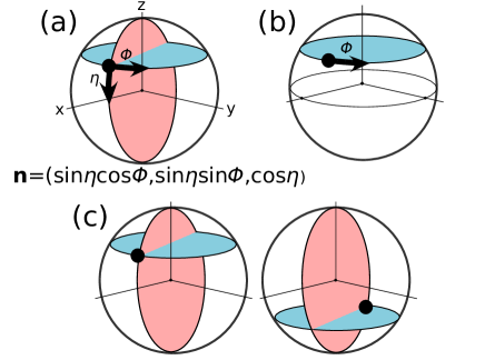
where is the vector of unitary Pauli matrices. The Bloch sphere representation of a spin is given in FIG. 3 (a). The mean Uhlmann curvature of model
| (118) |
is given by
| (123) |
Thus (118) is weakly commutative only at the north and south poles . We call the state and the model (118) as a spin and a spin model, respectively. The spin model turns weakly commutative with some modifications presented in FIG. 3 (b) and (c).
A.1.2 Off-equator phase estimation
Fixing the latitude of the spin to a constant results in a single-parameter model of phase . States of the single-parameter model
| (124) |
form a circle in the Bloch sphere with a constant latitude (a schematic representation is in FIG. 3 (b)).
The model does not have any GAS except at the equator . At the equator, the spin-flip followed by -rotation along the -axis becomes a GAS. Outside the equator, the circular orbits are passed to the other hemisphere by the spin-flip. There is no unitary to return the whole circles to the original hemispheres [86].
A.1.3 Antiparallel spins
Antiparallel spins are two spins directing the opposite to each other. A schematic representation is given in FIG. 3 (c). The antiparallel spin model is represented by
| (125) |
since the spin-flip operator flips a spin to its opposite direction.
Gisin and Popescu [53] showed that the spin direction can be better guessed from the antiparallel spins than from parallel spins. Later Chang et. al. [54] demonstrated the advantage of antiparallel spins for the estimation of spherical coordinates . The weak commutativity of antiparallel spins is shown there. Since the model consists of pure states, it must be quasi-classical [25].
The antiparallel spins has a GAS
| (126) |
where is the tensor product of spin-flips, and is the operator which swaps the sides of bipartite system . The antiunitary operator flips the directions of spins on both sides, and then unitary swaps the spins to recover the original state. The GAS (126) is a conjugation despite is not.
Depolarized antiparallel spins
| (127) |
are no longer quasi-classical, nor partially commutative (see Appx. A.1.4 for details). Nevertheless, the GAS (126) is preserved by the depolarized channel.
Let us consider the optimal POVMs for antiparallel spins. Vectors
| (128) |
with properly chosen four Bloch vectors () are known to form an optimal measurement basis for antiparallel spins [54]. Here, represents a state vector with Bloch vector (see [53, 54] for details on the phase factors). This set of vectors indeed satisfy
| (129) |
and thus is a reference basis that represents as a mere complex conjugation.
There are different reference bases for the same conjugation . An example is
| (130) |
where now represents the computational basis. Later we see that our basis (130) sometimes outperforms (128) in terms of the precision for depolarized antiparallel spins (Sec. 5.1). This is unexpected because the basis (128) provided by Gisin and Popescu [53] looks much specialized to the estimation of . In fact, each component of (128) is the optimal covariant measurement vector to maximize a fidelity measure for this specific problem [79].
A.1.4 Classical and quantum Fisher information matrices for antiparallel spins
We first show that the depolarized antiparallel spins is not quasi-classical. Then we present the deviation of single-parameter stemming from POVM measurements on depolarized antiparallel spins. The latter corresponds to the precision of the off-equator phase estimation on the depolarized antiparallel spins.
The state of depolarized antiparallel spins is defined by Eq. (127). A pair of SLDs for depolarized antiparallel spins is given by
| (131) |
for , where is the SLD for single spin, given by
| (134) | ||||
| (137) |
The SLD operators for the depolarized antiparallel spins is unique since the state is of full-rank. The commutator of SLD operators reduces to
| (138) |
This never becomes zero since is not proportional to . Thus the depolarized antiparallel spins is not quasi-classical. It is not partially commutative as being of full-rank.
The deviation can be calculated as the inverse of the classical Fisher information about . We here provide a full analysis on the two CFIMs for reference-basis measurements (128) and (130). Note that for general depolarized state and a projector , probability to have the corresponding result is
| (139) | |||
| (140) |
The -component of the CFIM is
| (141) |
The CFIM is calculated from the probabilities to obtain the result by the measurement on the original state.
Let us first consider the basis (128) given by Gisin and Popescu [53]. The probabilities to obtain result () can be found, for example, in the appendix of [54]:
| (142) | |||
| (143) |
The corresponding elements of CFIM for the depolarized antiparallel spins are given by
| (144) | ||||
| (145) | ||||
| (146) |
The deviation for this measurement is given by .
If our measurement (130) is applied on the pure antiparallel spins, the probabilities are
| (147) | |||
| (148) | |||
| (149) |
The corresponding elements of CFIM are given by
| (150) | ||||
| (151) | ||||
| (152) |
The deviation is again given by the inverse of .
The QFIM of pure antiparallel model is
| (153) |
where is the QFIM of single spin. While this relation can be derived by a direct calculation, it is expected by Eq. (106). The depolarization deteriorates QFIM to
| (154) |
Again the minimum of deviation is the inverse . This bound is the best attained by the (potentially target-dependent) optimal measurements each on a single copy of the depolarized antiparallel spin pairs.
We take the latitude as a constant and consider the single-parameter estimation of phase , which is trivially quasi-classical. This is the antiparallel version of off-equator phase estimation. The deviation based on the measurements in reference bases (128) and (130) is compared to the optimal deviation in FIG. 4.
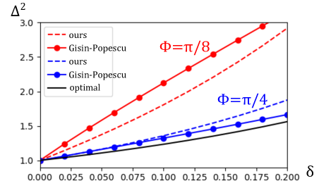
A.2 Qubit inside a disc
Suzuki [27] gave an weakly commutative model of a qubit
| (157) |
where and are arbitrary real functions of the parameter such that , and and are arbitrary (not necessarily orthogonal) unit vectors on -dimensional real space. In the Bloch sphere representation, the qubit is in a disc spanned by two vectors and . The disc cross the origin and cuts the sphere into halves. This model is not quasi-classical [27].
The qubit inside a disc (157) is imaginarity-free. The state transforms under the spin-flip as
| (158) |
Mutually opposite vectors and are always in the same plane which includes the origin . Thus the spin-flip followed by the unitary -rotation along this plane takes any state to itself.
It is crucial for the disc to cross the origin. Otherwise the model does not have a GAS.
A.3 Embedding quantum simulators
Here we introduce a class of model inspired by embedding quantum simulators [67, 68, 69, 70, 71, 72]. EQS model for pure state model is defined by
| (159) |
where
| (160) |
with some conjugation on , where is a two dimensional ancillary system with an orthonormal basis . The transformation is not realized as a completely positive map. Extra resources are required to produce the state .
The global phase subtlety matters when modifying to EQS models. The modifications to EQS models result in different models from and from where is a parameter-dependent global phase. While these two original models are equivalent, their EQS models demonstrates different precision bounds.
Embedding quantum simulators typically utilize the encoding of state in the form
| (161) |
instead of [67]. With (161) we arrive at the same precision bound since it is unitarily equivalent to .
A GAS of EQS model (159) is
| (162) |
where is the conjugation in the product basis such that (). A reference basis to represent (162) as a complex conjugation is
| (163) |
Thus a product measurement saturates QCRB.
QFIMs of EQS models are sometimes improved from the original models. QFIM of an EQS model relates to that of the original model by
| (164) |
where
| (165) |
is a real vector. It is futile to modify EQS models again to their EQS models to obtain even better precision bound. The second modifications are equivalent to mere unitary transformations.
Appendix B Local antiunitary symmetry
This section technically supports the discussion of Sec. 5.2 on LAS by providing proofs. We prove Thm. 4 in Sec. B.1. Section B.2 derives optimal local measurements from LAS. Section B.3 gives examples of quasi-classical models without any antiunitary symmetry.
Following lemma is frequently employed throughout this section.
Lemma 6
A model has a LAS at if and only if (1) holds and (2) there are set of SLD operators satisfying
| (166) |
at .
proof) Suppose has a LAS at . A set of SLD operators is defined by Eq. (9). These SLD operators satisfy Eq. (166) because and holds by the assumption.
Conversely, if and are -invariant, the defining equation (8) implies that is a LAS of at .
Note that if the density operator is of full-rank, then the SLDs are in one-to-one correspondence with the derivatives .
B.1 Proof of Theorem 4
We start by proving that any model with a LAS at is weakly commutative at . From Lem. 6, there are SLD operators satisfying Eq. (166). Then we have
| (167) |
because , and are all invariant under . This reveals the weak commutativity of at .
Conversely, assume that a pure-state model is weakly commutative at point . Since all pure weakly commutative models are quasi-classical [25], there is a set of SLDs satisfying
| (168) |
for any pairs of . Let be a basis of in which the SLDs are diagonalized
| (169) |
where are the real eigenvalues. We represent the state vector
| (170) |
with the real coefficients and phase ().
Define a new basis vectors by
| (171) |
for . The state is represented by a real matrix in this basis since . The SLDs are still diagonalized by the new basis. The derivative is also real in this basis since
| (172) |
holds for all . The complex conjugation in the basis is a LAS of at .
B.2 Optimal measurements from local antiunitary symmetry
Here we prove that rank- POVM that is invariant under LASs forms optimal measurement for local multiparameter estimation.
Theorem 5
B.3 Quasi-classical models without local antiunitary symmetries
We construct quasi-classical models without any LASs. According to Thm. 4, these examples are inevitably mixed-state models. We give two kinds of examples in Sec. B.3.1 and Sec. B.3.2. We also show that any quasi-classical qubit model has a LAS in Sec. B.3.3.
The following lemma is used in exhibiting the non-existence of antiunitary symmetries for both of the examples.
Lemma 7
Let be a real non-degenerate diagonal matrix. If remains real for a unitary , then is decomposed to
| (173) |
where is an orthogonal matrix and
| (174) |
with some set of phases .
proof) Let us denote the real matrix by . Since is diagonalized to by the inverse unitary , ’s columns must be unit eigenvectors of . Since the real Hermitian matrix is symmetric, its eigenvectors () can be taken real. Therefore is decomposed as
| (175) |
where are phases and is an orthogonal matrix.
The lemma follows by taking the Hermitian adjoint on both sides of Eq. 175.
The action of diagonal phase matrix as a similarity transformation is presented by
| (176) |
for arbitrary matrix .
B.3.1 Single-parameter model
We consider a qutrit model whose state is
| (183) |
where are different positive real constants that sum to , are constant phases, and is the parameter. Operator is a quantum state for sufficiently small . At we have
| (187) | ||||
| (191) |
We now prove that the model (183) does not have any LAS at for a proper choice of .
From Thm. 1, we can assume that the LAS is given by a conjugation. Therefore, it is sufficient if we prove that and cannot be simultaneously decomplexified by a unitary transformation.
Let be any unitary that makes real. Then is decomposed as Eq. (173) into a phase matrix and an orthogonal matrix (Lem. 7). For we have
| (192) |
from Eq. (176). The components of cannot be simultaneously real when
| (193) |
by any choice of the phases . Since is a real orthogonal matrix,
| (194) |
cannot be real for any choice of the phases and . This completes the proof of non-existence of LAS at .
B.3.2 Multiparameter model
Let be a -dimensional space and be a basis. Let be a full-rank density operator on . Define operators () by
| (195) |
so that holds for any , and holds for any pair. The operators can be identified to SLDs of a model with -parameters such that
| (196) | ||||
| (197) | ||||
Because is full-rank, are the unique set of SLDs for model at .
From Lem. 6 and the uniqueness of SLDs, has a LAS if and only if there is an antiunitary such that
| (198) |
holds. From Thm. (1), we can assume that is a conjugation. Since and hold for any conjugation, Eq. (198) holds for some conjugation if and only if and () are simultaneously decomplexified in a basis of .
Now, take as the reference-basis for matrix representations. By applying Lem. 7 to a non-degenerate real diagonal matrix (, for ), any unitary matrix that keeps real can be decomposed as to the diagonal phase unitary and an orthogonal matrix . The action of on is given by Eq. (176):
| (199) |
for all and . The density matrix is decomplexified by if and only if is real.
If , consider a density matrix such that
| (200) | ||||
| (201) |
hold. Equations (201) and (199) imply that the phase differences must make real for any and , if is real. For such a choice of phase differences, however, cannot be real from Eq. (200). Therefore, the density matrix satisfying Eqs. (200) and (201) cannot be decomplexified by . The model does not have any LAS at if we choose satisfying Eqs. (200) and (201).
B.3.3 Qubit model
If , any quasi-classical model have a LAS. For any qubit model, the maximum size of the set of mutually independent and commuting SLDs is [99]. Let () be the spectrum decomposition of the unique SLD . Again we take the basis as the reference for matrix representation. Choose two phases and so that
| (202) |
holds. Then the matrices and are simultaneously decomplexified by the phase matrix .
Appendix C Set imaginarity, set antiunitary asymmetry, and asymmetry measures for quantum statistical models
In this section, we consider measures of imaginarity and antiunitary asymmetry for a set of quantum states. The purpose is to later introduce corresponding measures for quantum statistical models. We employ measures of imaginarity from a resource theoretic framework reviewed below. Then the measures are extended to fit to our purpose.
C.1 Resource theory of imaginarity
Resource theories of imaginarity [60, 61, 62] start from specifying a reference basis . Then imaginarity-free states are determined as real density matrices in the basis. To fit to our discussion, we represent the set of imaginarity-free states as
| (203) |
where is the complex conjugation in the reference basis . Measures of imaginarity quantify how much a given state differs from imaginarity-free states. The measures must satisfy monotonicity under imaginarity-free operations (operations that does not affect imaginarity-free states [60]), and return zero for imaginarity-free states. Hickey and Gour proposed the distance measures
| (204) |
and the robustness of imaginarity [60]. If we choose the trace distance, the distance measure is expressed in a closed-form
| (205) |
and is faithful, meaning that they are strictly positive outside the imaginarity-free states. The robustness later turned out to be equal to [61, 62].
C.2 Set imaginarity
The imaginarity thus defined is measured in terms of a fixed basis , or equivalently a fixed conjugation . In contrast, the weak commutativity is implied by any conjugation. In our sense, a model should be called “imaginarity-free” if the states are simultaneously real for some reference basis which is not fixed in advance. We are looking at a basis-independent definition of imaginarity.
Such a definition of imaginarity has not been studied yet. However, there is a basis-independent definition of coherence [92, 93, 94] termed “set coherence” [95]. We follow the procedure to define “set imaginarity,” and “set antiunitary asymmetry.”
A set of quantum states is presented by . The free set is given by
| (206) |
for each . It is a union of free sets for fixed conjugations defined by
| (207) |
Completely analogously to set coherence [95], we may define max-distance
| (208) |
and mean-distance
| (209) |
as measures of set imaginarity. These measures are faithful when we choose the trace-distance because is faithful for the basis-dependent imaginarity. We do not touch operational meanings of the measures thus defined. A measure of set coherence inherits an operational meaning from basis-dependent coherence [95].
C.3 Antiunitary asymmetry
The procedure to define (basis-dependent) imaginarity generalizes straightforwardly to antiunitary asymmetry. The representation (203) of imaginarity-free states extends the states with general antiunitary symmetry
| (210) |
by replacing the conjugation to an antiunitary operator . The distant measures are generalized accordingly.
The set imaginarity and “set antiunitary asymmetry” are equivalent when defined by distance measures. Theorem 1 implies that for any antiunitary operator , there is a conjugation such that
| (211) |
and hence
| (212) |
hold for any distance measure. The set of free states for the set antiunitary asymmetry
| (213) |
is equal to the free set for imaginarity by Eq. (211). The max- and mean-distances
| (214) |
are equals respectively to and by Eq. (212). The difference between imaginarity and antiunitary asymmetry only appears at the basis-dependent definitions for distance measures.
C.4 Antiunitary asymmetry of quantum statistical models
There are many ways to define antiunitary asymmetry of a quantum statistical model at each point . We require the measure to be faithful: the measure must be zero only if there is a LAS at the point. The max-distance (208) inspires us to define
| (215) |
and call it max-imaginarity. Since the limit diverges unless , we have
| (216) |
In a similar way we define mean-imaginarity as
| (217) | ||||
inspired by the mean-distance (209). The imaginarity and the antiunitary asymmetry remains equivalent for these definitions.
Our asymmetry measure (115) is inspired by the mean-imaginarity (217). We are not sure if the measure is equivalent to
| (218) |
since we cease to use the trace distance.
Our asymmetry measure(115) has an advantage of being invariant under isometric coordinate transformations. Since the Jacobian of an isometric coordinate transformation is an orthogonal matrix , we have
| (219) |
where are the derivative with respected to the transformed coordinates.
I am not sure if there is a faithful asymmetry measure that is invariant under general normal coordinate transformations. The LASs, if they exist, are preserved by these transformations. Namely, a model has a LAS at if and only if
| (220) |
has a LAS at , where is any normal coordinate transformation. Methods to extend this invariance of antiunitary symmetry to asymmetry measures remain open here.
