Multiscale characteristics of the emerging global cryptocurrency market
Abstract
Modern financial markets are characterized by a rapid flow of information, a vast number of participants having diversified investment horizons, and multiple feedback mechanisms, which collectively lead to the emergence of complex phenomena, for example speculative bubbles or crashes. As such, they are considered as one of the most complex systems known. Numerous studies have illuminated stylized facts, also called complexity characteristics, which are observed across the vast majority of financial markets. These include the so-called “fat tails” of the returns distribution, volatility clustering, the “long memory”, strong stochasticity alongside non-linear correlations, persistence, and the effects resembling fractality and even multifractality.
The striking development of the cryptocurrency market over the last few years – from being entirely peripheral to capitalizing at the level of an intermediate-size stock exchange – provides a unique opportunity to observe its evolution in a short period. The availability of high-frequency data allows conducting advanced statistical analysis of fluctuations on cryptocurrency exchanges right from their birth up to the present day. This opens a window that allows quantifying the evolutionary changes in the complexity characteristics which accompany market emergence and maturation. The purpose of the present review, then, is to examine the properties of the cryptocurrency market and the associated phenomena. The aim is to clarify to what extent, after such an impetuous development, the characteristics of the complexity of exchange rates on the cryptocurrency market have become similar to traditional and mature markets, such as stocks, bonds, commodities or currencies.
The review introduces the history of cryptocurrencies, offering a description of the blockchain technology behind them. Differences between cryptocurrencies and the exchanges on which they are traded have been consistently shown. The central part of the review surveys the analysis of cryptocurrency price changes on various platforms. The statistical properties of the fluctuations in the cryptocurrency market have been compared to the traditional markets. With the help of the latest statistical physics methods, namely, the multifractal cross-correlation analysis and the -dependent detrended cross-correlation coefficient, the non-linear correlations and multiscale characteristics of the cryptocurrency market are analyzed. In the last part of this paper, through applying matrix and network formalisms, the co-evolution of the correlation structure among the 100 cryptocurrencies having the largest capitalization is retraced. The detailed topology of cryptocurrency network on the Binance platform from bitcoin perspective is also considered. Finally, an interesting observation on the Covid-19 pandemic impact on the cryptocurrency market is presented and discussed: recently we have witnessed a “phase transition” of the cryptocurrencies from being a hedge opportunity for the investors fleeing the traditional markets to become a part of the global market that is substantially coupled to the traditional financial instruments like the currencies, stocks, and commodities.
The main contribution is an extensive demonstration that, fuelled by the increased transaction frequency, turnover, and the number of participants, structural self-organization in the cryptocurrency markets has caused the same to attain complexity characteristics that are nearly indistinguishable from the Forex market at the level of individual time-series. However, the cross-correlations between the exchange rates on cryptocurrency platforms differ from it. The cryptocurrency market is less synchronized and the information flows more slowly, which results in more frequent arbitrage opportunities. The methodology used in the review allows the latter to be detected, and lead-lag relationships to be discovered. Hypothetically, the methods for describing correlations and hierarchical relationships between exchange rates presented in this review could be used to construct investment portfolios and reduce exposure to risk. A new investment asset class appears to be dawning, wherein the bitcoin assumes the role of the natural base currency to trade.
keywords:
Cryptocurrencies , Complexity measures , Cross-correlations , Fractals , Multiscaling , Complex networks , Lead-lag effect100
1 Introduction
Modern financial markets are characterized by a rapid flow of information. There is a huge number of transactions between market participants with different investment horizons. There are pension funds, for those time scale is years, and at the same time specialized algorithms operating at the level of seconds or even milliseconds (high-frequency trading). The market behaviour is the result of various influencing factors, ranging from economic data, results of companies, interventions of central banks, poll and referendum results, individual tweets of high-ranking people, and mutual interactions between participants. Through feedback, this leads to critical-like phenomena such as speculative bubbles or crashes. This happens often in hours or even minutes – the so-called “flash crashes”. These features undoubtedly fit into the characteristics of complex systems, such as a large number of elements, nonlinear interactions, structural self-organization, and emergent phenomena.
The first quantitative research on financial markets was the subject of Louis Bachelier’s work [1], in which he derived a formula for option price based on cumulative distribution function (CDF) of a stochastic process now called the Wiener process. Later Benoît Mandelbrot’s works turned out to be a groundbreaking achievement [2]. While examining cotton price fluctuations, he observed that, contrary to wide belief, their probability distribution function (PDF) is characterized by heavy, non-Gaussian tails. Mandelbrot was also the first to notice a fractal structure of stock price fluctuations.
More than a quarter century ago, statistical physicists started their serious research in financial markets, which led to an outburst of a new discipline – econophysics [3, 4]. Numerous studies carried out since then allowed researchers for a better understanding of the mechanisms governing various phenomena on both the macroscopic level (like speculative bubble formation, market crashes, asset cross-correlations, nonlinear autocorrelations, portfolio evolution, etc.) and the microscopic level (order book properties, efficacy of investing strategies, price formation, etc.). Along with the understanding, new models have been proposed that better describe and predict market behaviour and practical trading algorithms have been developed and applied especially in high-frequency trading.
All types of markets have been a subject of research since the beginning of econophysics: stock markets [5, 6, 7, 8], commodity markets [9, 10, 11], option and future contract markets [12, 13, 14], bond markets [15, 16, 17], real-estate markets [18, 19, 20], as well as the foreign currency market (Forex) [21, 22, 23]. Unlike typical complex systems studied by experimental physicists, these markets offer good quality data with minimum systematic errors, which is one of the reasons why so much attention they attract. However, there is an important issue that is inherently associated with all the above mentioned markets: they have already been existing for a long time before they become a subject of research. Therefore, we cannot investigate their evolution since their origin. Nevertheless, more or less a decade ago a brand new market was established – a cryptocurrency market, which offers precisely what the other markets lack – a possibility of observing their structural self-organization process from the very beginning to a rather mature form in a short period of time. A principal question is to what extent, after such dynamic development, complexity characteristics of the cryptocurrency market are similar to those of traditional markets, especially Forex.
The first cryptocurrency - Bitcoin (BTC) - was proposed in 2008 by a person or group of people under a nickname Satoshi Nakamoto [24]. The date of this new concept emergence does not seem to be accidental, because it is correlated with an epicenter of the global financial crisis of 2008-2010. In order to mitigate its effects, the central banks began to increase the monetary base (“printing money”) massively, which weakened trust in the traditional fiat currencies. The bitcoin protocol was based on a peer-to-peer network and the previously known public and private key cryptographic techniques together with a new consensus mechanism called “Proof of Work”. The idea behind bitcoin was to provide, for the first time in human history, a tool that would allow people anywhere to trust each other and carry out transactions via Internet without a central management institution. Instead of the current confidence in the state/central banks, confidence in technology was proposed.
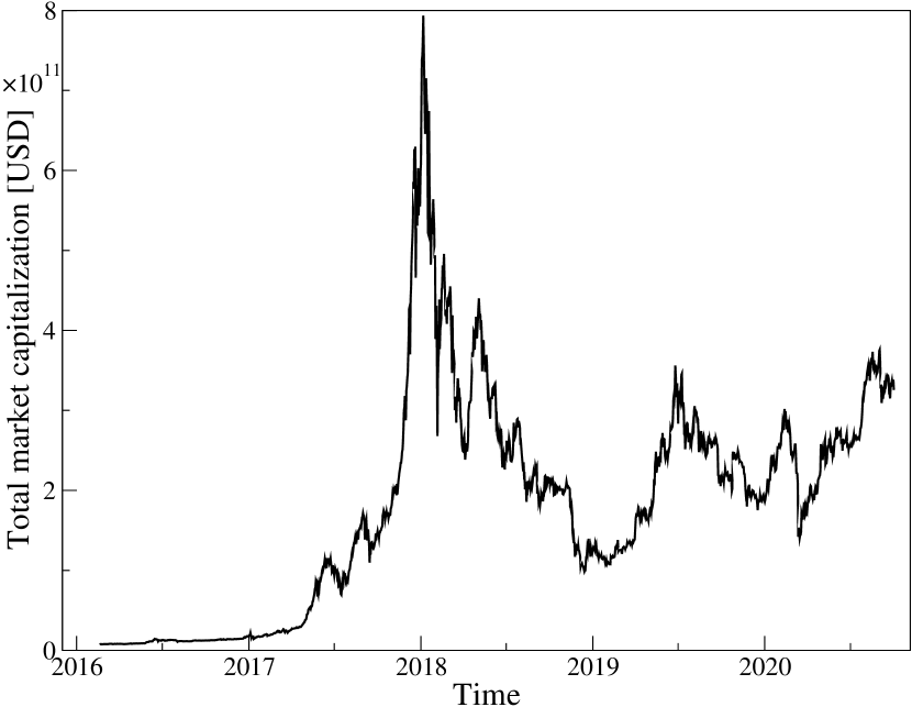
The first widely recognized platform offering BTC-to-fiat-currency exchange was Mt. Gox founded in Feb 2011. Since then a spectacular development of the cryptocurrency market has occurred. There are already 3,600 different cryptocurrencies traded on 350 platforms with nearly 30,000 cryptocurrency pairs listed. Current capitalization of the entire market is about 350 billion USD (Oct 2020 [25]). It increased rapidly in 2017 during a speculative bubble referred to as ICO-mania [26, 27] reaching over 800 billion USD in the beginning of 2018. BTC valuation on some Korean platforms was even 20 000 USD. Currently, the market is highly decentralized with the same cryptocurrency pairs listed on many platforms. There is no single price to refer to unlike that provided by Reuters on Forex. Only for BTC there are quoted future contracts launched in Dec 2017 on the CME group [28]. Another characteristic property is that cryptocurrency transactions are most often made through the platforms in contrast to Forex with its over-the-counter market.
Aim of this work is to review the available results on the cryptocurrency market obtained with various methods of statistical physics with the multifractal formalism and the network approach in particular. Our work sketches briefly history of the cryptocurrency introduction (Sect. 2.1) and describes the blockchain technology standing behind them (Sect. 2.2), but its main part presents a review of the most important properties of the cryptocurrency price fluctuations. Price return distributions, autocorrelations, and inter-transaction times of cryptocurrency exchange rates are compared with their counterparts in Forex (Sect. 3). Non-linear auto- and cross-correlations together with multifractal-like characteristics on the cryptocurrency market are then described. Among others, it is shown that PDF/CDF form, autocorrelation functions, Hurst exponents, and multiscale properties depend on trading frequency (Sect. 4). Cross-correlations among the cryptocurrency exchange rate pairs within one trading platform and between two platforms, as well as between the cryptocurrency platforms and Forex are also discussed (Sect. 5). Triangle arbitrage effects are a subject of Sect. 5.2.3. Latest Covid-19 pandemic impact on correlations between cryptocurrencies and traditional financial markets is covered in Sect. 5.4. The last part of this review discusses results of a network approach (Sect. 6). It is shown that, currently, BTC is a natural base cryptocurrency for other cryptocurrencies.
2 The emergence and technology of cryptocurrencies
2.1 History: from barter through the blockchain
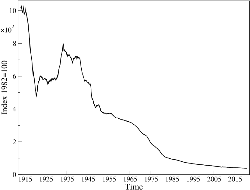
Human history has been paced by discrete events that shaped its course through discontinuously accelerating development. Without question, one of these events is the emergence of money in the form of standardized coins, which were introduced in Lydia around 600 years BC. This first generation of currency shaped Mediterranean culture in many ways [29], and spearheaded a continuous increase in trade exchanges. Merchants no longer had to resort to barter, good for good, or service for service. The second generation was paper money, which appeared in the Renaissance. It was introduced by Italian banks and subsequently taken over by the established national banks. The invention of banking and paper money disrupted the status quo of the feudal systems, by strengthening the nation-states which had the power to issue it. From this point onwards, the possibility of modulating the money supply upwards or downwards was easily available, eventually giving rise to modern capitalism [29]. The 20th century brought the appearance of electronic transactions, which further accelerated the circulation of currency throughout the economy, boosting growth. Crucially, paper and electronic money caused a total decoupling of fiat currencies from their fundamental value. After the collapse of the Bretton Woods system in 1971, exchange rates ceased to be linked to gold and based on trust in the state. From that point onwards, fiat currencies systematically lost their value, as shown for the example of the US dollar in Fig. 1. Moreover, since breaking with gold as a reference, the number of USD in circulation has kept increasing systematically, as visible in Fig. 2.
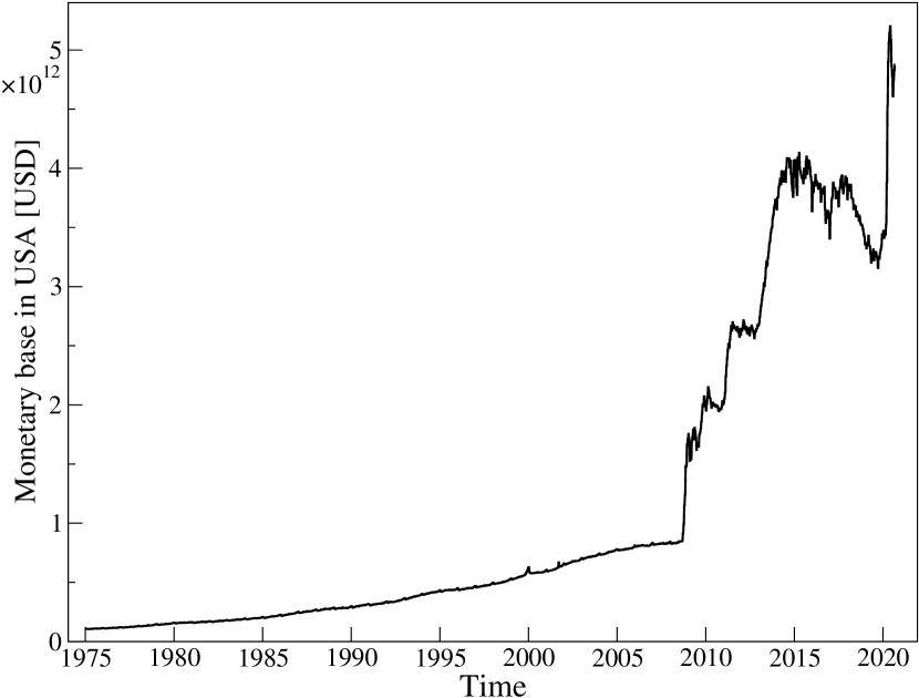
Currently, central banks can easily increase the supply of currency without any physical printing. After the financial crisis of the year 2008, all the major central banks significantly expanded their monetary base through quantitative easing programs (QE), as visualized in Fig. 2. Incidentally, around the same time, a radically new financial asset appeared. That was the first cryptocurrency, the Bitcoin [24]. The underlying revolutionary idea was to combine existing technologies in a novel way, namely asymmetric cryptography, together with a distributed database having a new “Proof of Work” consensus mechanism into a decentralized, secure register (the distributed ledger technology, DLT) blockchain [31].
The intention is that cryptocurrencies are not subjugated to any institution or government; rather, they are based on trust in technological infrastructure. They allow sending financial resources anywhere in the world with almost zero latency. The network users themselves provide the authentication mechanism. The cryptocurrency concept combines the advantages of cash, namely the transaction anonymity, with the speed and convenience of electronic transactions. Importantly, unlike traditional currencies, the Bitcoin by design has a built-in supply limitation mechanism, which helps prevent its loss of value.
Initially, the Bitcoin seemed to be only a technological curiosity, and there was no organized trade. Individual transactions for exchanging real goods via on-line discussion groups were described, such as buying two pizzas in May 2010 for 10,000 BTC [32]. However, the innovative idea soon began diffusing outside its original circle of computer geeks, extending towards the broader financial sector and, eventually, by virtue of the anonymity, also to criminal circles. The first widely recognized exchange, which enabled bitcoins to be traded for traditional currencies, Mt.Gox, was launched in July 2010. Soon after, the first on-line black market, Silk Road, was created: it allowed virtually unregulated trading of any goods, bolstered by bitcoin payment and full anonymity. Perhaps concerningly, this was the first practical application of the Bitcoin. It significantly increased demand and contributed to the first speculative bubble on bitcoin prices [26], which burst after Silk Road was shut down by the FBI in October 2013 and trading by the largest cryptocurrency exchange, Mt.Gox, was halted in February 2014, plausibly after a hack which led to the disappearance of 850,000 BTC.
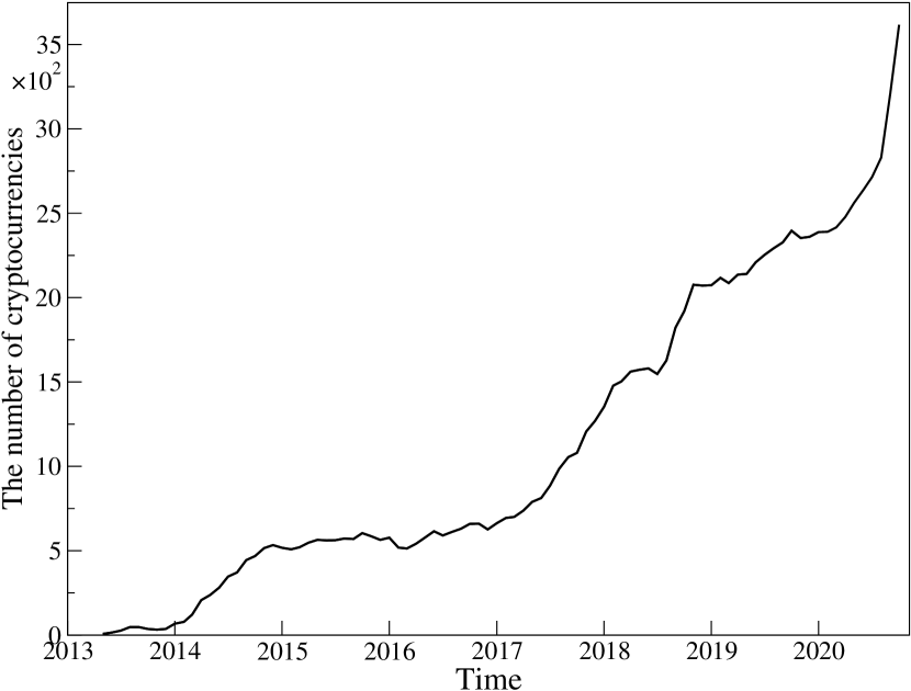
As recognition increased, the technology became increasingly widespread. Eventually, it turned out that the blockchain technology on which cryptocurrencies are based allows using for a decentralized registry not only for financial purposes but also for the execution of computer code (scripts) in a distributed form. At the end of 2013, the idea of an Ethereum distributed computing network was introduced. The project started in July 2015 [33]. The Ethereum platform allows anyone to create decentralized applications operating without the possibility of downtime, censorship, fraud, or tampering with their code. It also allows one to issue their own tokens via smart contracts, which consist of computer code performing a prescribed action under certain conditions on the Ethereum blockchain. This innovation quickly found application in raising capital via a simplified mechanism for various projects through the so-called Initial Coin Offer (ICO). In 2017, the ICO underwent a boom, which contributed to another speculative bubble on the cryptocurrency market, referred to as the ICO-mania [27]. At that time, the number of cryptocurrencies doubled from 700 to 1,400 by the end of 2017 (figure 4), and the capitalization of the entire market reached USD 800 billion (figure 5). Unavoidably, the bubble eventually burst in January 2018.
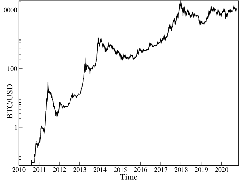
The current state of the blockchain technology can be compared to the dot-com bubble at the turn of the century. The considerable potential was already visible in the then possibilities of the Internet, but it was not known precisely which particular way the technology would develop. At that time, merely mention a company’s intention to engage in Internet-related activities would cause a sharp increase in share price [34]. A similar case was verified for the cryptocurrencies. With the first euphoric phase now well over, the bitcoin from top to bottom in December 2018 lost over 80 percent of its value (figure 3). Other cryptocurrencies have dropped by as much as 99 percent, with some unavoidably succumbing. Currently, the first practical applications of the blockchain are emerging; these will be discussed alongside the mechanics of cryptocurrencies in the next sections.
2.2 Core technology
The most straightforward approach for dispatching “electronic cash” would be using data files. However, digital data can inherently be replicated unlimitedly, which engenders a double-spending problem. Therefore, there was a need for a technology that could form an electronic register covering all transactions: transferring funds would, then, consist of swapping entries in the register. This type of record is commonplace in the electronic banking system, but central to the notion of a cryptocurrency was the aim of abandoning their central character, rendering them completely public instead. In this way, each user could verify transactions independently, yielding another valuable property, namely the impossibility of corrupting the registry history. This challenge was resolved through the use of peer-to-peer (P2P) networks, cryptographic techniques, and connecting transactions in blocks, and after that in a chain of blocks, the blockchain. In this section, without losing generality, the underlying technology will be presented, taking as an example the first cryptocurrency, the Bitcoin.
2.2.1 The network
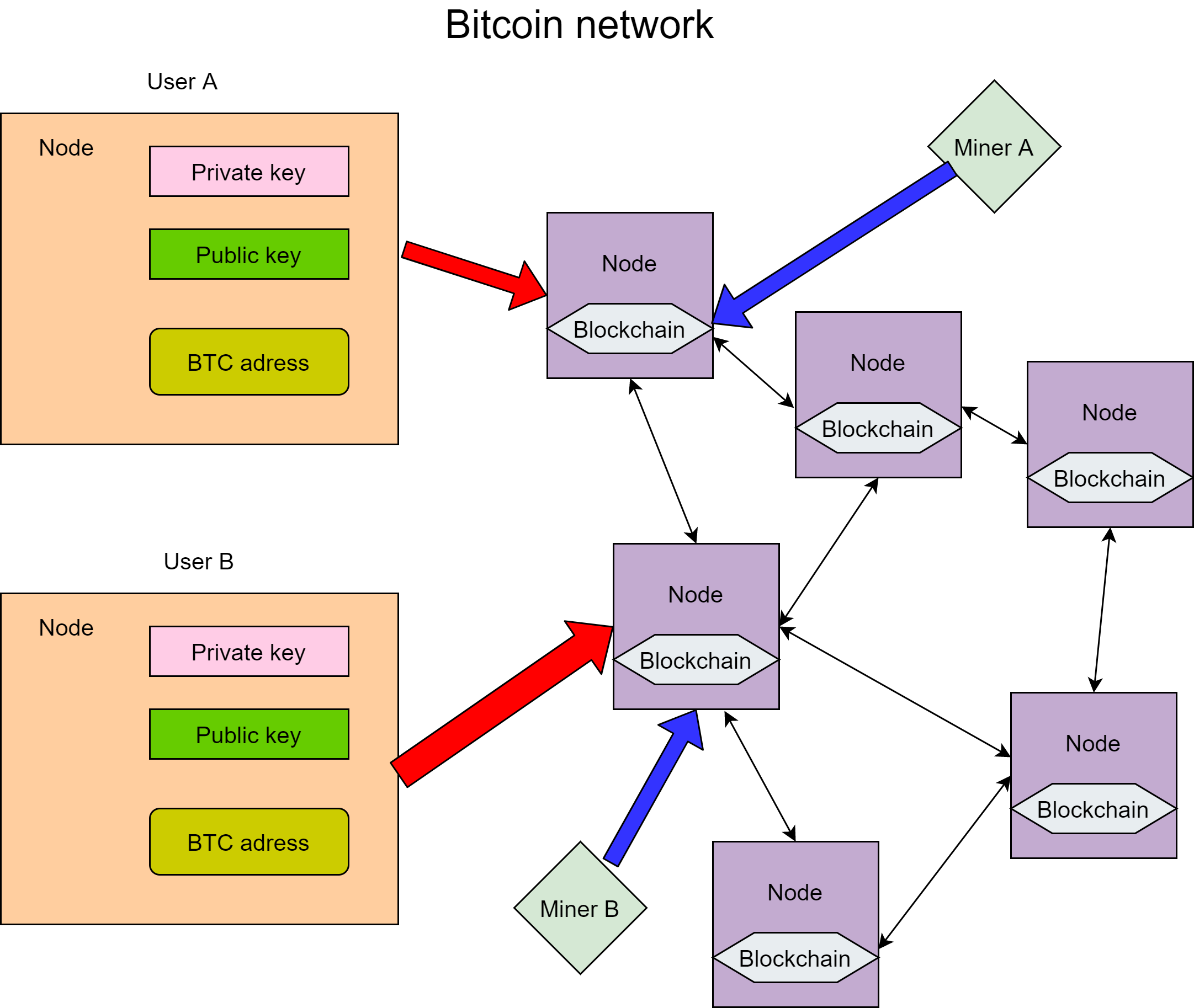
The Bitcoin is a virtual monetary entity and, as such, is devoid of any physical form. The minimum unit is 0.00000001 BTC (1 satoshi). Bitcoin blockchains are data files that contain information about past transactions and about the creation of new Bitcoins, providing a means of reward for closing a block with transactions. This is known as the Bitcoin network register. The blockchain consists of a sequence of blocks, wherein each subsequent block is built upon the previous one and contains information about new transactions in the network. The first block was created in 2009. Currently, as of October 2020 the chain counts nearly 650,000 blocks. As said, the Bitcoin blockchain is public: everyone can access all information about how many BTCs belong to a given address in the network. Further, the registry is not centralized: all network participants have their own blockchain copies and can modify them. There is no supervisory unit; however, there is a set of rules that each user must follow. As a consequence, the participants reciprocally control each other. To enter the Bitcoin network, a prospective user must use a network client or an external wallet. Enacting a transferring implies sending to the network information indicating that the recipient address is now the owner of the specified BTC amount. This information is distributed in a capillary form until all nodes have been informed about the transfer. Throughout this process, transaction integrity is provided by asymmetric cryptography, wherein the private key encrypts the transaction by the sender, and the other network users can read the message via the public key. In other words, this means that each transaction can be ascribed to a precise actor because no other has access to their private key. When information circulates through the network, everyone can read it but not re-encode an altered transaction. The scheme for sending BTC in the network is represented in figure 6. Each transaction is coded via the hash function, which for Bitcoin is dSHA256 [35].

For a virtual currency, the fundamental substrate to functioning is a means of determining how many units are circulating at any time-point and how many will be created. There must exist a consensus mechanism ensuring that all users agree to the ownership of the virtual currency. In the Bitcoin network, wherein users remain anonymous and do not have to entrust each other, proper operation requires that all nodes maintain consensus regarding the current state of the system among themselves. Most participants in the distributed network must agree and perform the same action: the Bitcoin’s key innovation is a mechanism that allows large-scale compliance of users on the network, solving the so-called Byzantine generals problem [36].
For the network to function efficiently, there is a need for entities that collect transactions, ascertain correctness, and combine into potential blocks: these are known as miners. As a reward for their activities, they receive an amount in newly-created Bitcoins alongside a usually small transaction fee, debited after block approval and inclusion in the primary chain. This happens when most network participants have reached a consensus to add a block candidate in their copy of the blockchain. Anyone can become a miner. The only requirement is the client software and the latest copy of the network registry. However, due to the sheer computational cost of the validating block process, miners arrange themselves into so-called “Mining pools” and make use of tailored high-performance computing solutions based on graphics processing units (GPU) or application-specific integrated circuits (ASICs) [37]. To be accepted, a new block must meet specific criteria. The result of the hash function, namely dSHA256 for the case of the Bitcoin, when applied to the data contained in the block must have a unique property: it must begin with a predetermined number of zeros. The number of starting bits resulting from hashing function which must be zero reflects the difficulty of confirming blocks. Miners collect transactions from the network (Fig. 8) and search for a number called “nonce”, given which the hash function will return the result with the specified number of zeros at the beginning. If they succeed, they immediately send their block to the network, and the other users can easily verify its correctness. The consensus mechanism among miners is that any miner who receives a new block from the corresponding result of the hash function (hash) includes it in the blockchain. From game theory, a strategy wherein all miners add correct blocks to their copy of the blockchain is Nash’s equilibrium state [38]. In other words, insofar as a miner believes that everyone else is acting fairly, their best option is to add a block to their copy. Operations on a blockchain version that is are not universally accepted are economically unprofitable because there is no reward for simply creating new blocks in it. This arrangement results in a consensus regarding the state of ownership of Bitcoins throughout the network, despite the absence of a centralized manager.
When confirming subsequent blocks, commonly known as “mining Bitcoins”, financial costs are incurred in the form of electricity consumption and the necessity to have specialized equipment. Nonce, the number required for closing a block, can be obtained only through an iterative process, i.e., a closed-form equation is prohibited by the formulation. For this reason, the consensus mechanism is referred to as a proof-of-work (PoW). Finding the correct result of a hash function with a specific number of zeros at the beginning requires, on average, a huge number of calculations [37]. Adding incorrect information (e.g., fictitious transactions) to the candidate for a block would cause his rejection, simply dissipating the energy used for the calculations. This is the reason finding the correct result from hashing is proof that a miner helps maintain the Bitcoin network.
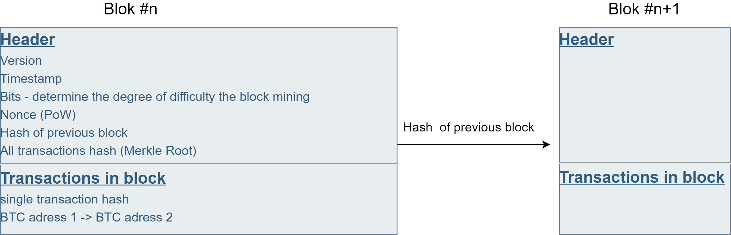
Because each subsequent block contains the header from the previous one, it is impossible to alter past transactions without rebuilding the entire chain. Due to the time, difficulty, and cost of finding the right result of the hash function, it is economically unviable. The blockchain diagram is shown in Fig. 7. The Bitcoin protocol was created in such a way that the algorithm adjusts the difficulty in finding the right result of the hash function to the network computing power, so that a new block is created on average every 10 minutes [35]. The maximum block size is 1 MByte, determining how many transactions it can contain. As said, for the inclusion of a new block into the blockchain, miners receive a prize in the form of newly-created Bitcoins. The reward in halved every 210,000 blocks, up to the limit of 21 million Bitcoins [35]. It is possible that two miners would simultaneously and independently produce a new block and include it in their copy of the blockchain, causing multiple versions to appear. Such occurrences are dealt with applying the longest chain rule, i.e., the one for computing which the larger amount of power was invested is retained. This is a fundamental preservation mechanism. The pool rejects the shorter one during confirmation, and the miner receives no reward. A consequence is that blockchain technology is susceptible to so-called 51% attacks. When a miner has control over more than half of the computing power in the given network, they can confirm blocks faster than anyone else, thus manipulating transactions in the nearest attached blocks. The cost of carrying out such an attack on the Bitcoin network and other PoW-based networks was obtained in Ref. [39].
A limitation of the Bitcoin protocol is its low efficiency and the high costs of proof-of-work mechanism, which ensures network security. The primary costs are the non-recurring investment in computing power and the ongoing cost of electricity, which is currently at the level of that consumed by entire countries, such as Ireland and Denmark [40]. Another issue is the low network capacity. Bitcoin can handle, on average, only five transactions per second (TPS) [41]. By comparison, the Visa circuits handle on average about 1700 TPS [42]. In other words, one of the foundational advantages of the blockchain technology, namely the inability to make arbitrary changes to the blockchain, also results in a core rigidity. If one performs a transaction, this needs to be propagated to the entire network, and the previous version of the chain needs to be discarded, leading to the so-called “hard forks”. It should be noted that the Bitcoin protocol is not static, as it is subject to constant modifications. To date, a mechanism reducing the transaction size has been introduced, known as the “SegWit” (segregated witness), which packing more transactions into each lock. Work is currently underway on the introduction of the “Lightning Network”, which would allow micropayments to take place outside the main chain and thus which would increase network bandwidth, albeit at the price of reduced security.
2.2.2 Methods for attaining network-wide consensus
The near totality of cryptocurrencies are predicated, like the Bitcoin, on the initially-introduced proof-of-work (PoW) consensus algorithm. It protects against external attacks, however, it is inefficient. For this reason, faster algorithms have been developed and are being trialled. The second most popular algorithm after proof-of-work is the proof-of-stake (PoS) alongside its various modifications. Unlike with PoW, no miners are competing for calculating as soon as possible the right hash function value closing a block. Instead, the next block’s validator is a pseudo-random node from the network, the precise choice being based upon a combination of factors potentially including randomness and how many cryptocurrency units a given node has.
According to the PoS algorithm, blocks are “forged” and not mined as in the case with the PoW mechanism. Blockchain networks based on proof-of-stake also make use of transaction fees as rewards for “forgers”. However, whereas in the case of networks based on proof-of-work the reward for miners reward is a newly created cryptocurrency unit, in proof-of-stake networks the users who want to take part in the forging process must block for some time the number of cryptocurrency units in the network as a “stake”. The assumed rate’s size determines the chances of choosing a given node as the next validator, which will check the next block. The higher the stake, the higher their chances are. For the selection process not to favor only the richest, additional selection methods are added to the network. The two most commonly used are randomized block selection and coin age selection.
Every cryptocurrency using the proof-of-stake approach has its own set of rules determining who will become the validator of the next block. Security in the PoS algorithm is implemented via the built-in possibility of losing a blocked stake and the right to participate in future transactions as a punishment of passing a fraudulent transaction. As long as the stake remains higher than the reward, the validator will lose more cryptocurrency units than they would have gained when attempting to commit fraud. As for the PoW protocol, the PoS algorithm is vulnerable to 51% attack [43]. Such an attack can be perpetrated when a network node possesses more than half of the supply of a given cryptocurrency. In that case, they can then approve fraudulent transactions. The main advantage of the PoS algorithm is its efficiency. As the need for computationally-demanding calculations is relieved, no specialized user groups are needed to confirm blocks, enabling it be done faster than as compared to PoW.
A variation of the PoS algorithm is known as the delegated proof-of-stake (DPoS) [44]. It is based on the notion that the owners of a given cryptocurrency outsource block processing work to a third party. The latter are known as the so-called delegates, for whom the network users can cast votes, and who secure the network if they win the election. Their task is attaining consensus during the generation and approval of new blocks in the network. The weight with which each network user decides about its future during voting is proportional to the number of the units of a given cryptocurrency that they possess. The voting system varies depending on the project, but usually, each delegate presents an individual proposal related to their plan for the development of the network and then asks for votes. As a rule, rewards received by delegates for creating and confirming blocks are proportionally shared with their voters. Therefore, the DPoS algorithm is based on a voting system directly dependent on the reputation of delegates. If a selected node (delegate) does not work efficiently or breaks the rules, it is removed, and another one is selected in its place. In terms of performance, networks using DPoS are more scalable. As the number of users increases, they can process more transactions per second compared to networks using PoW and PoS algorithms. The next section surveys the Bitcoin protocol modifications and other possible blockchain technology applications in further detail.
2.3 Cryptoassets and diversified applications of the blockchain technology
A core aspect of the Bitcoin protocol is its open-source form: consequently, anyone can review, analyze, and copy the specifications, resulting in a rapid spread of the new technology. At first, mere Bitcoin clones were created, sharing the same network structure with minor modifications such as block size, hash function, mining limit, and creation time for new blocks. However, as the blockchain technology developed, novel projects expanding its use cases rapidly emerged. For instance, they allowed not only saving the transaction register but also executing code computer code in the form of a script. Throughout the impetuous development of the cryptocurrency market and all possible uses of blockchain technology, the original concept of a cryptocurrency began blurring. A more general concept was introduced: cryptoassets, which could be classified in three categories as a function of the applications: cryptocurrencies, cryptocommodities, and tokens [45].
Cryptocurrencies denote the first use of the blockchain technology and are intended to transfer funds. Modifications of the Bitcoin protocol are the most common. The first to maintain a significant position today is Litecoin (LTC), created in 2011. It is a clone embedding two changes. The first consists of reduced time between block extractions by a factor of four times and an increased maximum limit to 84 million, allowing a substantial increase in the speed of transaction confirmation [42]. The second is the use of another hash function, known as scrypt, which is more appropriate for implementing on standard processors for confirming blocks in the Litecoin network instead of requiring ASIC as in the case of Bitcoin.
The first cryptocurrency not based on the Bitcoin protocol was the Ripple [46], created in 2012. It does not implement the PoW consensus mechanism, implying that there are no miners in the network. Instead, it relies on a partially-centralized system called trusted nodes, which are responsible for confirming transactions. The idea behind Ripple is to provide connections between banks and stock exchanges to send money in real-time, which would entail using Ripple instead of fiat currencies for transfers outside national borders. Ripple tokens (XRP) were released by Ripple Labs. It currently owns most of this cryptocurrency. Currently111The data presented in this section are from October 2020., XRP is the fourth cryptocurrency in terms of capitalization. Its main competitor is Stellar (XLM), which also supports transactions between financial institutions. Unlike Ripple, the protocol is open source type and based on an own token. Both XRP and XLM tokens do not have a fixed supply limit and are, therefore, subject to inflation.
Since the Bitcoin blockchain is public and one can trace the transaction history of each mined coin, it is not entirely anonymous. The answer to this “drawback” was the emergence of cryptocurrencies ensuring complete undetectability to their users, the so-called “private coins”. This group of such cryptocurrencies includes: Dash, Monero, and Zcash. Dash (DASH) has a hybrid architecture based on two network layers: the first involves miners using the PoW mechanism, as in the case of Bitcoin, the second comprises the so-called “masternodes” using the PoS technique. Monero (XMR) ensures anonymity thanks to a RingCT, by which the addresses (public keys) of those who make transactions are hidden in the blockchain. It is considered the cryptocurrency providing the most significant anonymity and, as such, is regrettably in widespread use by criminals, for example, for demand ransom payments [47]. Zcash (ZEC) is based on a “zero-knowledge” protocol called ZK-Snarks. It is a cryptographic solution that allows confirming whether the information is correct without having to disclose it, thus ensuring the anonymity of both the sender and recipient of a transaction to be preserved, while concealing its entity. Anonymous addresses are called shielded addresses and are compatible with public addresses, such that one can perform a transaction from a public wallet to a protected one and vice versa. Zero-knowledge is also used by cryptocurrencies such as ZClassic (ZCL), Bitcoin Private (BTCP), PIVX, and Komodo (KMD). In the cryptocurrency group protecting anonymity, Dash and Zcash have a built-in maximum supply mechanism, whereas Monero does not.
The so-called cryptocurrency group also includes several Bitcoin hard forks. The Bitcoin Cash (BCH) represents the first Bitcoin division, wherein part of the community decided to disconnect and develop the project on a new blockchain. It entails increasing the block size from 1 to 8 MBytes, and then to 32MB. In the next division, Bitcoin Gold, the hash function was changed to Zhash, allowing efficient block confirmation on non-specialized hardware. Another variation, Bitcoin SV, stems from Bitcoin Cash and features a block size of 128 MBytes.
The second category of cryptoassets, cryptocommodities, serve as the basis for applications of the blockchain technology. They are “material” enabling the creation of decentralized applications and smart contracts. These are automatically executed computer codes that perform specific actions when certain conditions are met. Cryptocommodities operate as “fuel”, allowing one to pay for using a decentralized computing network.
Ethereum [33] was the first realization of such an idea. It was proposed in 2013 and launched in 2015 as an open-source computing platform based on the blockchain. It has been equipped with its own programming language, known as Solidity, through which one can program smart contracts and decentralized applications. It has its cryptocurrency called ether or ethereum (ETH), which serves as a payment unit for carrying out computational operations. Their price is expressed in the so-called units of “Gas” and depends on the computational complexity necessary to complete an operation. Ethereum, like Bitcoin, is based on blockchain technology and the PoW consensus mechanism. However, it uses another hash function, Ethash, that supports the efficient use of GPU hardware in the mining process. It does not have a fixed block size. Instead, each block requires a specific number of Gas units, which determines the computing power needed to complete the transactions it contains. The average time between blocks is about 15 seconds, and the maximum number of transactions per second is around 25. Unlike for Bitcoin, there is no upper limit on mining. In the future, the developers predict a transition to a PoS consensus mechanism, which would increase network bandwidth.
The Ethereum concept gained considerable popularity among the cryptocurrency community from the outset. In 2014, 18.5 million USD were collected from pre-sale, hallmarking the highest result of crowdfunding at that time. This result was beaten by a venture capital fund, the DAO, which aimed to raise capital for the development of blockchain startups and non-profit organizations. The fund took the form of a decentralized, autonomous organization built on the Ethereum blockchain in an intelligent contract. In 2016, it collected 11.5 million ethereum worth nearly 168 million USD. On this occasion, one of the pros/cons of blockchain was revealed, namely code unchangeability. It turned out that the DAO smart contract code had gaps that allow unauthorized funds to be transferred. A hacker attack took place in June 2016, during which 3.6 million ethereum were stolen. To reverse the effects and change the DAO code, the Ethereum blockchain had to be split. On the new, the withdrawal of funds was canceled, whereas on the old, now called Ethereum Classic (ETC), everything remained unchanged. Currently, the ethereum remains the second cryptocurrency in terms of capitalization.
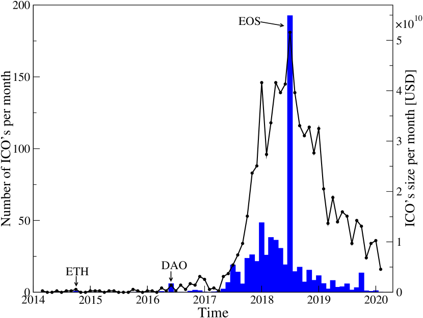
The considerable success of the concept of smart contract, in particular the possibility of collecting funds under the Initial Coin Offer (see Fig. 9) on the Ethereum platform, spearheaded competition also offering the possibility of creating applications in a decentralized computing network. Major projects of this type include EOS and Cardano. The EOS [49] platform is based on the delegated proof-of-stake algorithm (DPoS). As there is no mining process, unlike with Bitcoin or Ethereum, the network can process up to 15,000 transactions per second. However, this is attained at the expense of security. Only 21 selected block producers are responsible for verifying transactions, who receive awards in the form of newly created EOS units for their activities. The maximum number of EOS tokens is set to one billion units. The programming language used on the platform is known as WebAssembly. The leading EOS network was launched in June 2018, hallmarking the most substantial ICO offer in history. In year-long offer, ended in June 2018, it raised 4.2 billion USD eclipsing the world’s biggest initial public offerings of the year and more than doubling the next biggest offering of that type (see Fig. 9).
On the other hand, Cardano [50] uses the PoS algorithm, known as Ouroboros. There are two independent layers of the network: billing and computational. The accounting layer is built upon the blockchain network. The Haskell programming language is used to create intelligent contracts. The maximum supply of ADA cryptocurrency is 45 billion units. Other platforms offering similar services as Ethereum are the Tron – TRX, Lisk – LSK, ICON – ICX. They are similarly based on the DPoS algorithm. PoS-based platforms are Tezos, NEO (called the Chinese equivalent of Ethereum), NEM (based on Proof of Importance - a variety of PoS), and Waves. As one can see, it is typical for cryptocommodities to move from the original PoW consensus mechanism towards PoS, since this allows faster processing of network operations, which is required for additional than transaction-register functions.
The third group are tokens, which are the youngest cryptoassets and can be referred to as direct applications of blockchain technology. They are most often used as means of payment in decentralized applications (dApps) built on cryptocommodities such as Ethereum or are issued in the ICO offers for the development of a blockchain venture. Typically, they don’t have their own blockchain. Blockchain technology, thanks to eliminating a central intermediary who earn on commissions can be used wherever there is possibility to connect sellers and buyers directly (for example Uber and Airbnb).
The combination of token and cryptocurrency categories denotes the so-called “stable coins”. Their exchange rate is usually related to fiat currency. The most popular is tether [51] (USDT), which linked to the US dollar in a one-to-one relationship. It relies on Bitcoin blockchain via the Omni Layer platform and is issued by the private company Tether Limited, which declares that its supply is fully covered in US dollars. Other notable stable coins are the DAI, PAX, TUSD, and USDC.
The latest applications of blockchain technology are so called decentralized finance (DeFi). This term refers to an ecosystem of financial applications that are built on blockchain networks. Most DeFi platforms take the form of decentralized apps (dApps). They use smart contracts to automate financial transactions. The idea behind DeFi is to create decentralized cryptocurrency borrowing and lending system and to provide monetary banking services [52]. The largest projects of this type are: Chainlink, Wrapped Bitcoin, Uniswap, Maker and Compound.
2.4 Cryptocurrency trading
Cryptocurrencies, as a new concept, would not have much value in the early stages of their existence if they could not be exchanged for traditional currencies. One of the first exchanges that offered such opportunities was the Mt.Gox, as mentioned earlier, but the present cryptocurrency market is profoundly divided and decentralized. Nowadays222The data presented in this section are from October 2020. there are 350 cryptocurrency exchanges around the world. Most of them are platforms trading only cryptocurrencies with each other, with transactions performed around the clock. This is a key feature distinguishing the cryptocurrency market from the Forex, wherein trading occurs only from Monday to Friday. The second fundamental difference lies in the form and participants of the trade: in the case of cryptocurrencies, it takes place mostly between individual investors [53], whereas on the Forex, trading takes place on the OTC (Over-The-Counter) market and its participants are mainly banks. The third difference is the lack of a reference price, which in the case of the Forex market is provided by Reuters. Only in the case of the bitcoin, there is a futures contract quoted on the CME Group [28].
The decentralization of the cryptocurrency market means that the same cryptocurrency pairs are traded on different exchanges. Historically, significant valuation differences could be observed between exchanges [54]. For the stocks, this issue has been investigated and is called “dual-listed companies” [55, 56]. However, in the case of cryptocurrencies, which can be sent almost immediately between anywhere in the world, it represents a different kind of issue. The topic of trade comparison between cryptocurrency exchanges and arbitrage opportunities is covered in Sections 3.2 and 5.2.3. A common feature between the Forex and the cryptocurrency market is the possibility of triangular arbitrage [57, 58]. This will be discussed in detail in Section 5.2.3. A separate category not found in traditional financial markets is the so-called decentralized exchanges (DEX), where cryptocurrencies, through smart contracts, can be traded automatically, without any reliance on a central exchange server [59].
The statistical properties of the exchange rates of major cryptocurrencies will be analyzed in this review, considering the Binance, Bitstamp, and Kraken exchange rates. Binance [60] is currently the largest cryptocurrency exchange in terms of volume value. It was founded in July 2017 in China. After the regulation regarding trading in cryptocurrencies was tightened, the head office was moved to Malta in March 2018. At its inception, only cryptocurrency trade was conducted on it. Binance offers the ability to make transactions using approximately 800 different cryptocurrency pairs and additionally owns a cryptocurrency called the binance coin, which is used for paying commissions on the exchange. The exchange also offers the opportunity of carrying out ICO offers on it. Furthermore, daughter companies allowing exchanging cryptocurrencies for fiat currency. The Kraken exchange [61] was launched in September 2013, with headquarters in San Francisco and branches in Canada and Europe. It is the largest exchange in terms of volume value on cryptocurrency pairs expressed in Euro and currently offers 185 cryptocurrency pairs. The Bitstamp exchange [62] is one of the longest-running cryptocurrency exchanges. It was established in August 2011, and its head office of the exchange is in Luxembourg. The platform offers trading only on the most liquid cryptocurrencies, currently supporting 38 exchange rates.
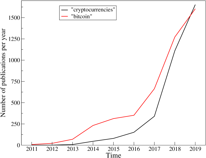
There was a sharp increase in the number of actively traded cryptocurrencies in 2017 (Fig. 4). Since then, the number of ICO offers has kept increased systematically (Fig. 9). The market capitalization also increased spectacularly, heralding the speculative bubble phase [26]. At the time of writing, approximately 3600 cryptocurrencies and nearly 30,000 exchange rates are present on the market [25]. The capitalization of the entire cryptocurrency market is on the order of 350 billion USD, and therefore comparable to middle-size stock exchange and largest American companies [64]. The spectacular development of the cryptocurrency market has attracted worldwide interest in the new asset, including the scientific community. The first works on the Bitcoin were published already in the period 2013-2015 [65, 66], but the real boom has only occurred since 2017 (figure 10). At first, scholars mainly examined the characteristics of the first cryptocurrency, the bitcoin [67, 68, 69]. Next, the community developed an interest in comparing it to other cryptocurrencies [70, 71, 72], which was followed by studies revealing correlations within the cryptocurrency market [73, 74, 75, 76, 77, 78, 79, 80] and its relationships to mature markets [81, 82, 83, 84, 85]. In particular, the possible uses of the bitcoin as a means of diversifying an investment portfolio and as a hedging instrument for the currency market [86], gold and commodities [87] and stock markets [88, 89, 90] were considered. A more detailed review of existing literature devoted to research on cryptocurrencies in the context of financial markets is available in Refs. [91, 92].
3 Statistical properties of fluctuations
3.1 Data
The presentation of results begins with the statistical properties of cryptocurrency price fluctuations from a brief description of the empirical data sets. Three issues are of interest here: (1) the cryptocurrency prices expressed in regular (fiat) currencies: US dollar and euro, with particular focus on bitcoin (BTC) as the most liquid and the most frequently traded cryptocurrency, (2) the cryptocurrency-cryptocurrency exchange rates, and (3) result comparison for two independent trading platforms.
The data were collected from the following sources. For BTC, the oldest cryptocurrency, the longest series of historical data was obtained from the Bitstamp exchange platform [62], offering the BTC price tick-by-tick quotes covering the interval 2012-2018 and expressed in USD. While the cryptocurrency market was expanding, more and more exchanges were created over time. They allowed trading not only BTC with USD, but also other cryptocurrencies with regular currencies, and even cryptocurrencies among themselves. A comparison between the properties of bitcoin and ethereum (ETH) was possible based on tick-by-tick quotes obtained from the Kraken platform [61]. The quotes covered an interval from mid-2016 to the end of 2018. A data set with quotes representing some less liquid cryptocurrencies, like litecoin (LTC) and ripple (XRP), unavoidably has to be smaller and covers only the entire year 2018, during which their trading frequency was sufficient to construct time-series without excessive constant-value intervals. To compare the properties of data from the different trading platforms, there is also consider a parallel set of the cryptocurrency quotes from Binance, the largest platform of this type. However, the sampling frequency of this set is 1 min, which provides us with 463,000 quotes for each exchange rate.
As a benchmark representing the regular currencies from the Forex, the EUR/USD exchange rate was considered, with quotes obtained from a broker, Dukascopy [93]. However, there is a significant difference between this dataset and the cryptocurrency datasets: the former excludes weekends and holidays, whereas the latter are recorded continuously.
In the following, three principal characteristics are reported: the average inter-transaction time (when available), which is denote by , the probability distribution function (PDF), and the autocorrelation function for the returns, defined as logarithmic exchange rate change over a fixed time interval : , where is an exchange rate of two distinct currencies or cryptocurrencies at time . The autocorrelations of both the signed returns and absolute returns (volatility) are of interest.
3.2 Average inter-transaction time
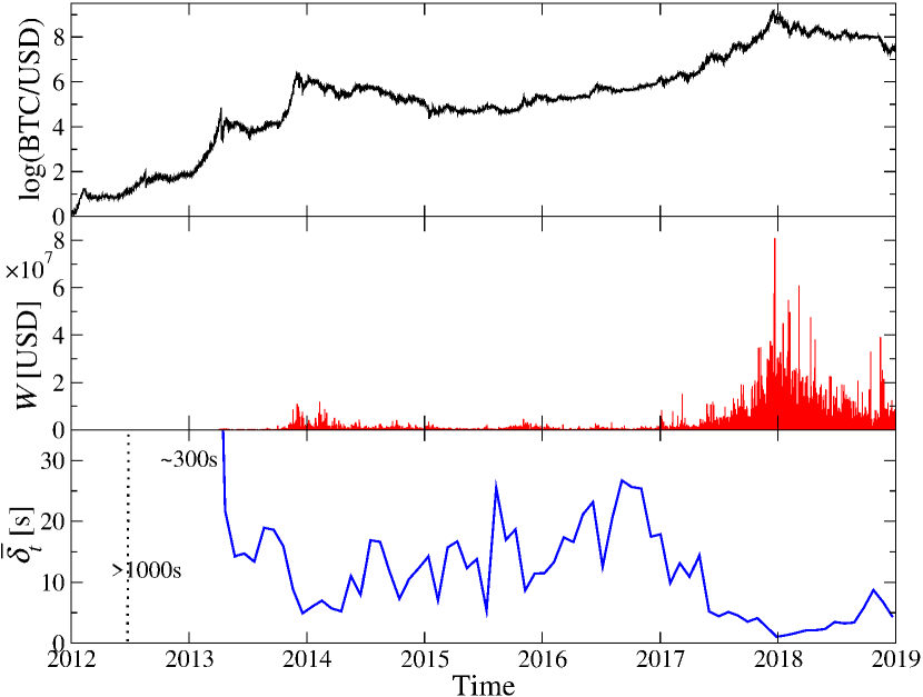
The analysis starts with the tick-by-tick quotes of the BTC/USD exchange rate as it is the most liquid and frequently traded cryptocurrency asset (Bitstamp quotes). Figure 11 shows the BTC/USD exchange rate, the BTC volume (in USD) traded during hour-long intervals, and average inter-transaction time calculated over monthly windows. There is an upward trend of BTC/USD throughout the years until the turn of 2017 and 2018. The trend was accompanied by a volume increase and a reduction in the average inter-transaction time. In 2012 and the first half of 2013, the trade volume was negligible. Subsequently, the peak of the first bull phase, at the turn of 2013 and 2014, was accompanied by an increase in volume and a reduction in the inter-transaction times. A side trend dominated the BTC/USD rate over the next three years and was associated with a volume decline and less frequent trading. A resume of the bull market towards the end of 2016, with spectacular growth in 2017 in particular, brought a further substantial increase in volume accompanied by a decrease in the average inter-transaction times. At the peak of the speculative bubble, at the turn of 2017 and 2018, the time between transactions became as short as around a second. A subsequent bear market caused a decrease in volume, which, however, remains above the pre-crash level observed in 2017. The average inter-transaction time was also affected but remains below 10 seconds.
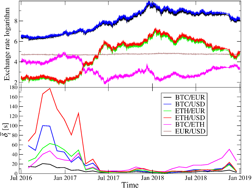
The mutual exchange rates (logarithms, top panel) and the inter-transaction intervals averaged over monthly windows (bottom panel) for the BTC, ETH, USD, and EUR based on the Kraken and Dukascopy data are shown in Figure 12. In parallel with Figure 11, one observes a gradual shortening of for the cryptocurrencies down to below 10 seconds in the bull-market phase (between mid-2017 and a trend reversal in early 2018). On the contrary, in the bear-market phase of 2018, a decrease in the BTC and ETH valuation in regular currencies was accompanied by an increase in . Only for BTC/EUR one still observed s. By looking at the exchange rate fluctuations over time, one can notice the considerably lower volatility of EUR/USD, almost resembling a flat line in the scale of Figure 12, as compared to the cryptocurrency-involving rates.
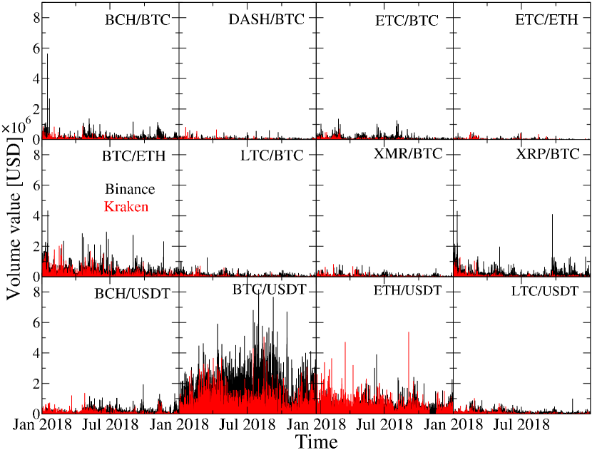
No strictly analogous result could be shown for the Binance dataset since it does not contain tick-by-tick quotes. Instead, the trading frequency can be related to the average length of intervals without trade (zero-return sequences) and the number of periods without trading. In Figure 13, the volume time-series from both exchanges were compared for 12 exchange rates involving both the most liquid cryptocurrencies (BTC, ETH) and the least liquid ones (DASH, XMR, LTC, XRP, BCH). Since on the Binance platform, the cryptocurrency value may only be expressed in terms of other cryptocurrencies, to facilitate the inter-platform comparison, the USD has to be replaced by a proxy – Tether (USDT), whose USD-based exchange rate fluctuates closely around 1. Therefore, the ETH/USD on Kraken corresponds to ETH/USDT on Binance. Figure 13 shows that a higher 1-min volume is seen on Binance for all exchange rates under consideration, which implies that the average inter-transaction time on Binance is shorter than on Kraken (see Table 1 in Sect. 3.3). The volume accumulates principally in BTC/USD and BTC/USDT, and then on ETH/USDT, BTC/ETH, and XRP/ETH.
3.3 Fluctuation distributions
At the dawn of scientific interest in the financial markets, it was believed that a normal distribution [1] could approximate the PDF of the stock market returns. Later, it was discovered by Benoît Mandelbrot that such distributions have significantly heavier tails and comply with the stable Lévy regime [2]. Consequently, the truncated Lévy distributions began to be used in this context [94]. Currently, it is accepted that, in mature financial markets, the CDFs of the absolute normalized returns in the bulk part develop fat tails of the form
| (1) |
where with and denote, respectively, sample mean and standard deviation. This relationship with different values of has been reported for many different asset types, including shares, currencies, commodities, and cryptocurrencies [5, 6, 95, 23, 96, 97, 68, 58, 98].
In particular, high-frequency stock-market data is frequently described by an inverse cubic dependence [99, 6, 100], i.e., the one with . A well-known fact is that the tail thickness of the return PDFs/CDFs decreases as increases from second to minute, hour, and longer scales [101, 102, 71]. A normal or exponential distribution can already approximate the return distributions for daily data. On the other hand, the return distributions for over the range of a few seconds are closely matched by the power-type functions [101]. This can easily be explained by the central limit theorem, provided the returns are independent: as increases, the distribution should converge to a normal distribution [103].
In general, it often happens that the fluctuations of a power-law type are associated with some critical phenomenon that occurs in the dynamics of a given system. However, in the financial market case, it was pointed out [104] that such behaviour of the return distributions might be related solely to the finite-size effects in the number of active agents and, therefore, any particular form of a power-law PDF may be viewed as accidental and non-universal [105, 106], opposite to what was believed earlier [100].
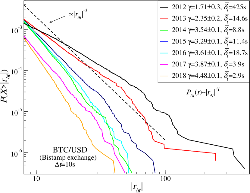
In order to calculate the cumulative probability distribution function (CDF), the tick-by-tick datasets from Bitstamp and Kraken were transformed to time-series of normalized returns , at a sampling frequency s. For the Bitstamp BTC/USD rate, it provides one with returns. As the analyzed period of 2012-2018 features diversified dynamics, the statistical properties of the returns have to be considered separately for each year. Figure 14 presents the CDFs of the absolute normalized returns. A power-type relation of the distribution tail (Eq.(1)) is observed for each year, at least over a part of the available return magnitudes, with the widest scaling range apparent in 2012. However, one has to notice that even in this latter case the power-law scale range does not exceed 1.5 decade, while its width gradually decreases each year and it falls well below one decade in 2018. This suggests that it is safer to consider these CDFs as only carrying some signatures of the power-law distributions and not being precisely the power-law ones.
There is evolution of the exponent from lower () towards higher values (), and the opposite trend for the estimation error. Furthermore, there is a relation between the shortening of the average inter-transaction time and the growing tail index , hallmarking a phenomenon observed in other financial markets as well. This relation can be interpreted as defining the internal time-flow of the market: the faster the trading and the shorter the inter-transaction intervals, the faster is the time-flow experienced by the assets and, consequently, the shorter are time-scales over which particular effects are observed [101]. The acceleration of market evolution is, therefore, a natural consequence of both the technological advances and the increasing market-participant influx that conjointly lead to higher transaction frequency. For example, for s, the return CDF tails for the BTC/USD, which were initially in the Lévy-stable regime with , became gradually thinner with in 2014 and in 2018 (figure 14). At present, the inverse-cubic scaling has to be addressed for a sampling frequency of s.
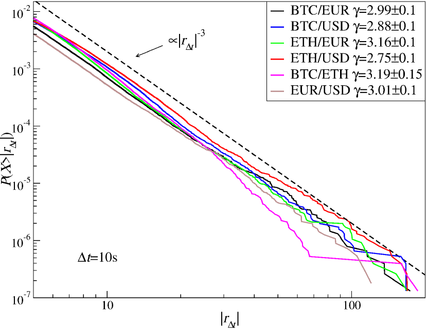
A comparison between the CDFs obtained for different exchange rates is presented in Figure 15 based on five return time-series from Kraken, namely BTC/USD, BTC/EUR, ETH/USD, ETH/EUR, and BTC/ETH (s, ), alongside the EUR/USD return time-series from Dukascopy (s, ). Here, the data covers the entire available interval, from mid-2016 through end-2018. Except for BTC/ETH, the distributions show a near power-law decay over about one decade, with the scaling exponent dwelling around . The values are slightly below this level for the BTC/USD and ETH/USD; these are the rates that, in a first part of the period under consideration, experienced the smallest trading frequency, with s. The BTC/EUR and ETH/EUR returns are characterized by that is the closest to 3, in parallel with the much more liquid Forex pair, EUR/USD, while the BTC/ETH crypto-crypto rate shows a slightly faster decay with .
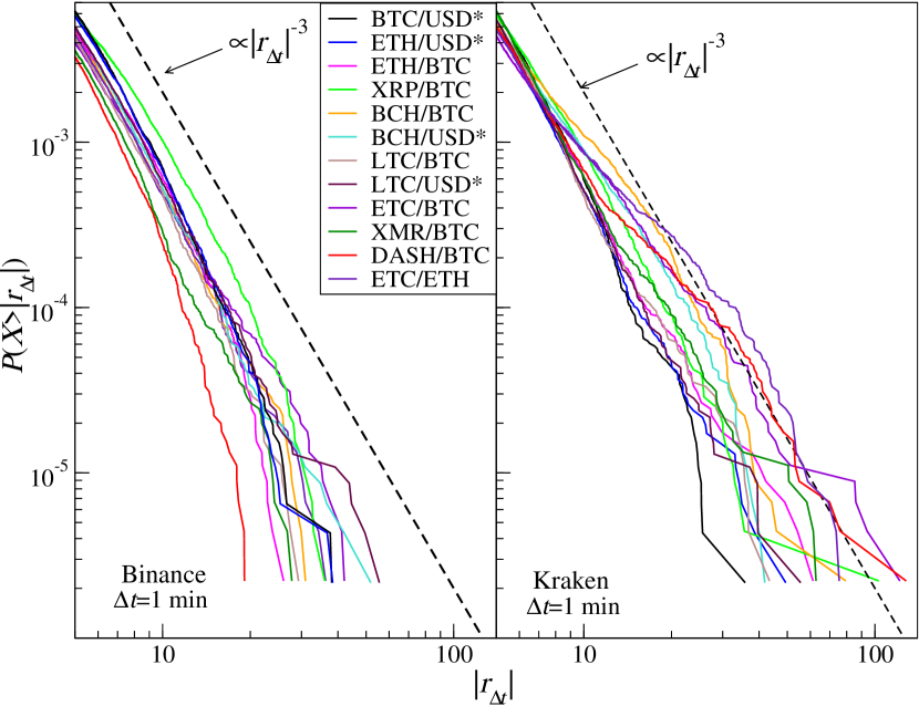
The results for the two different platforms, Kraken and Binance, are collated in Figure 16 and Table 1. By decreasing the sampling frequency to min (Jan-Dec 2018, ), the fluctuations of BTC and ETH can be compared with those of a few among the least-liquid cryptocurrencies, namely, XRP, BCH, LTC, XMR, DASH, ETC (all cryptocurrencies alongside their tickers are listed in the Appendix A). The exchange rates on Binance are characterized by a higher trading frequency (i.e., shorter average length and lower average number of non-trading periods, Table 1) compared to their counterparts on Kraken (see also Fig. 13). This affects the values of the exponent: while on both platforms, the exchange rate returns form CDFs with , the CDF tails for the exchange rate returns on Binance tend to decay faster than their counterparts on Kraken. This pattern is also discernible in Figure 16 and is in line with the observation that the trading frequency is related to the inner time-pace of a market. The less liquid exchange rates from Kraken have a slower internal time and, consequently, their rates of return distributions are characterized by thicker tails and poorer scaling (i.e., larger estimation error). By contrast, the CDFs for the rates with a higher trading frequency and volume resemble those characterizing the mature financial markets.
| [USD] | ||||||||
|---|---|---|---|---|---|---|---|---|
| Name | Bi | Kr | Bi | Kr | Bi | Kr | Bi | Kr |
| BTC/USD∗ | 3.450.1 | 3.630.15 | 1.07 | 1.61 | 8559 | 55360 | 196331 | 33998 |
| ETH/USD∗ | 3.390.1 | 3.40.1 | 1.10 | 1.78 | 16184 | 67807 | 61430 | 19711 |
| BTC/ETH | 3.300.1 | 3.180.2 | 1.09 | 2.62 | 12134 | 82074 | 60824 | 5250 |
| XRP/BTC | 2.910.1 | 2.990.15 | 1.20 | 3.50 | 41043 | 72556 | 31510 | 2763 |
| BCH/BTC | 3.360.1 | 2.350.15 | 1.25 | 4.39 | 29973 | 68059 | 16299 | 1251 |
| BCH/USD∗ | 3.360.1 | 2.610.15 | 1.40 | 3.83 | 40922 | 75427 | 15893 | 2151 |
| LTC/BTC | 3.420.1 | 3.340.15 | 1.17 | 5.09 | 34360 | 62675 | 13110 | 940 |
| LTC/USD∗ | 3.230.15 | 3.410.1 | 1.29 | 3.48 | 45208 | 79983 | 11793 | 1725 |
| ETC/BTC | 3.020.1 | 2.310.2 | 1.56 | 6.34 | 76691 | 55647 | 10164 | 709 |
| XMR/BTC | 3.680.15 | 3.210.15 | 1.37 | 6.58 | 47852 | 54832 | 4176 | 614 |
| DASH/BTC | 4.040.15 | 2.520.2 | 1.46 | 7.58 | 55684 | 49134 | 2777 | 416 |
| ETC/ETH | 3.340.1 | 2.180.2 | 2.30 | 9.15 | 82458 | 41861 | 1333 | 266 |
| Average | 3.380.11 | 2.930.16 | 1.35 | 4.66 | 40922 | 63785 | 35470 | 5816 |
Summarizing, it can be argued that, for a given exchange rate, in order to meet the characteristics typical of mature financial markets like the inverse-cubic dependence, a sufficiently high trading frequency is required. From the vantage point of the s, for the most liquid BTC/USD exchange rate on the Bitstamp platform, this was achieved in 2014; by contrast, on the Kraken the exchange the rates involving some of the least-liquid cryptocurrencies appear to be still in a “pre-cubic” immature phase.
3.4 Temporal autocorrelations
Another standard characteristic used to describe the financial returns is the autocorrelation function
| (2) |
where denotes the time-average. A typical behaviour of for the financial returns is its immediate decay either to zero or to below zero [107, 6, 108, 109, 23]. However, the autocorrelation function of volatility (i.e., absolute value of the returns) decays with an increasing according to a power law [110, 6, 111, 112, 113, 23]. The decay range corresponds to the average width of the volatility clusters [114]. This phenomenon, which can be observed across all markets, is a manifestation of long-term memory [96]: large fluctuations are statistically followed by large ones and small fluctuations by small ones [2]. The long-range autocorrelation, which is a linear effect in volatility, becomes a nonlinear correlation from the perspective of returns. Importantly, this implies that the returns can reveal multiscaling (see Section4).
It should be borne in mind that the autocorrelation function is a well-defined quantity only insofar as the data are drawn from a stationary process. Thus, if there is a trend in the data, it has to be removed beforehand. This also includes trivial periodic patterns. In the high-frequency financial data, one observes, for example, significant seasonal trends in volatility, including daily trends, weekly trends, and some longer-period trends. It is well-established that a satisfactory method of trend removal entails dividing each return corresponding to a time-point by the standard deviation of the returns calculated for the same moment over a sufficient number of trading days, i.e., , where indexes the intervals starting from the market opening.
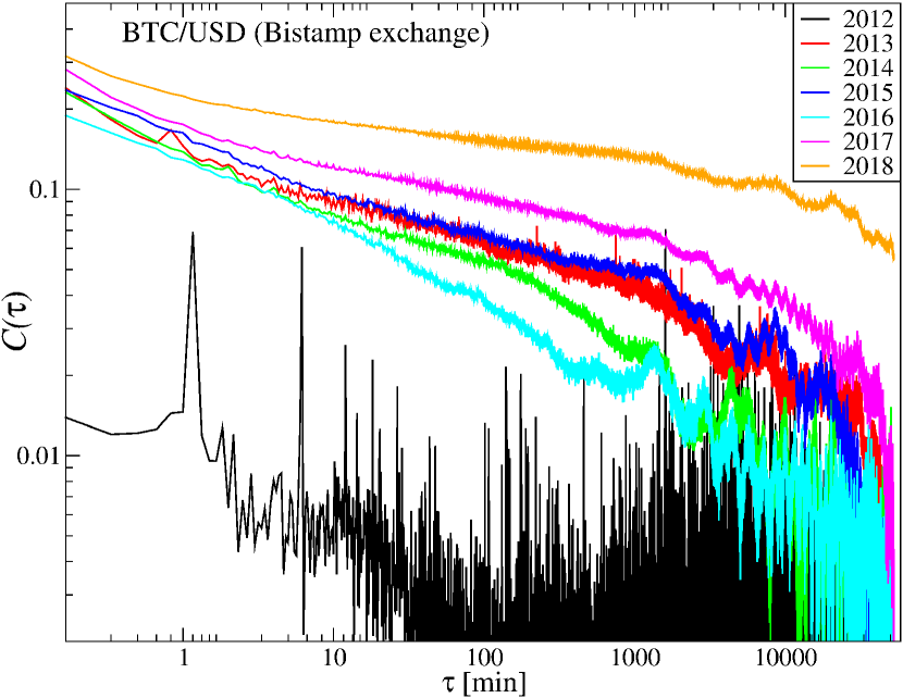
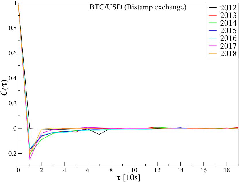
Figure 17 shows the autocorrelation function calculated for the BTC/USD volatility time-series split into annual parts. The quotes from the Bitstamp platform were first converted to absolute logarithmic returns, then detrended to remove seasonality. Similar to the CDF tails, a significant shift in the autocorrelation is observed between 2012 and the subsequent years. In the former, is only short-range correlated, with memory disappearing after a few minutes. However, long-range memory has a power-law form: accordingly, started to emerge already in 2013 and was systematically built up to reach substantial strength even for intervals as long as min by 2018. The effect of increasing the volatility autocorrelation time can be explained in terms of the increasing number of transactions carried out in a time unit.
The long-range, linear autocorrelation in volatility corresponds to non-linear correlations on the level of signed returns. In turn, non-linear correlations are responsible for the multifractal effects (see Sect. 4).
On the other hand, the autocorrelation function calculated for the original, signed returns does not indicate any linear memory effects for s (Figure 18). A negative value of is a statistical artifact related to isolated price jumps followed by price regression to a former level; these events are frequent on sampling frequencies comparable to the average inter-transaction interval. The observed autocorrelation function behavior for both returns and volatility resembles their counterparts on the other mature markets.
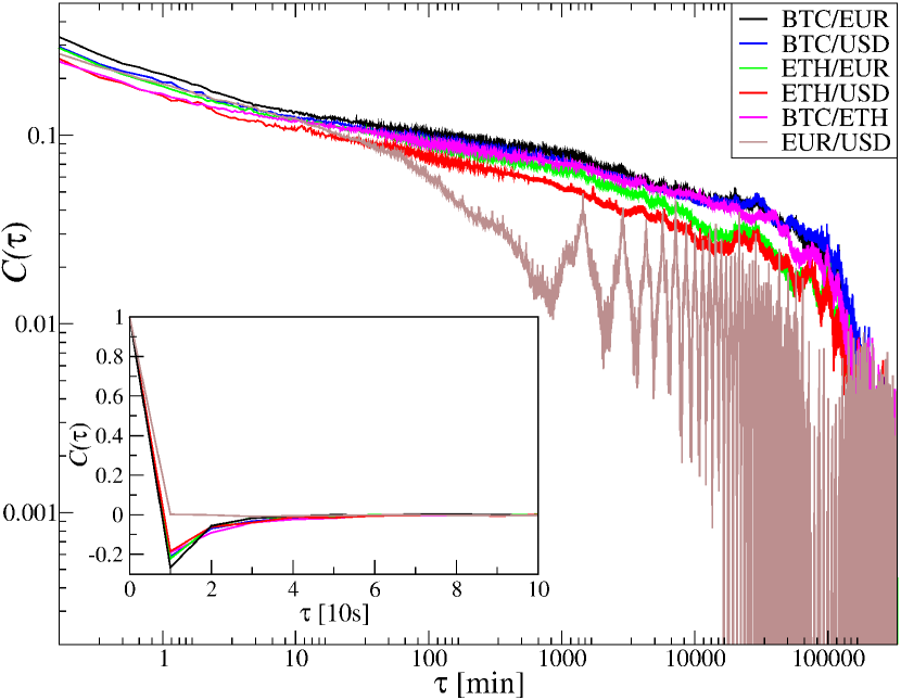
The volatility autocorrelations function for the BTC and ETH expressed in USD and EUR, as well as for BTC/ETH (Kraken), are displayed in Figure 19. For all cryptocurrency exchange rates under consideration, it decays with approximately according to a power-law up to about a week. However, in the case of EUR/USD (Dukascopy) the power-law regime breaks after already about one day, which can be accounted for by a shorter volatility-cluster length. This effect can be seen in Figure 20, where with s are shown for six exchange rates over the analyzed period. For the rates involving cryptocurrencies, the cluster length is an order of magnitude larger than for EUR/USD. Five cycles of high/low volatility during a week can be distinguished for the EUR/USD, while only three cycles per month are visible for the cryptocurrencies (insets in Fig. 20). Again, this can be explained by a higher trading frequency on the Forex than on Kraken. The average inter-transaction time is a few seconds on Kraken, whereas Forex transactions take place at least an order of magnitude faster.
Similarly to Bitstamp BTC/USD data, and indeed to all mature financial markets, the autocorrelation function for the returns (inset in Fig. 19) drops immediately to zero for the EUR/USD and even below zero for the cryptocurrency rates, indicating that no linear correlation exist for the signed returns.
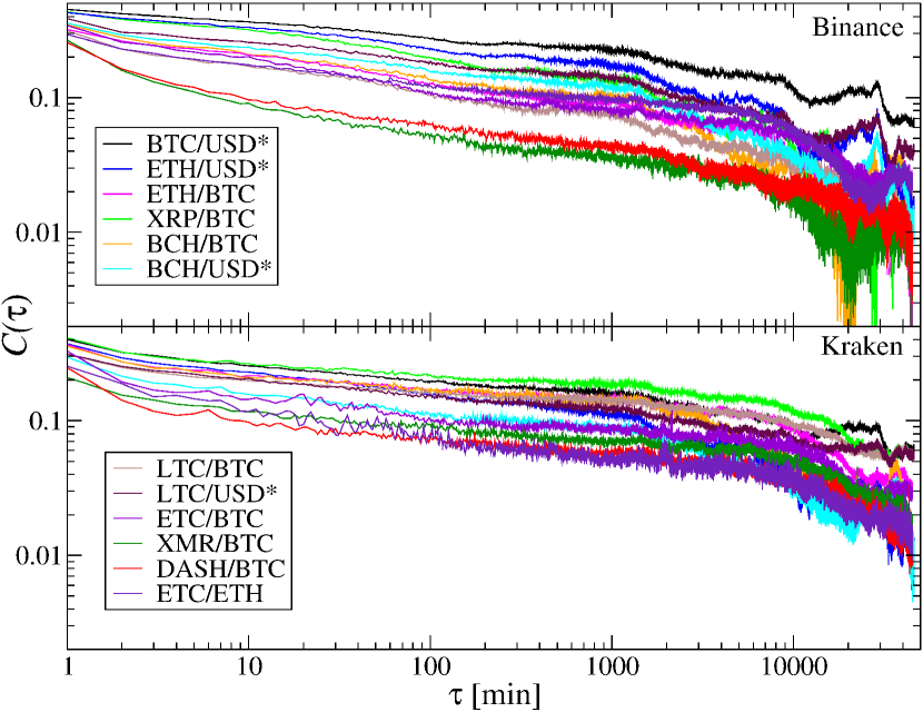
The difference in average trading frequency between Binance and Kraken affects not only the return CDFs but also the volatility autocorrelation function. In both cases, one observes its power-law decay (Figure 21), but on Binance, it is faster: it breaks down already after about 1,000 minutes as opposed to about 10,000 on Kraken. In the case of signed returns, the autocorrelation function exhibits a typical behavior: it immediately drops to negative values and then oscillates around zero (not shown).
4 Multiscale correlations
The commonly used correlation measures in time-series analysis, such as the autocorrelation function, the spectral density [115] and the Pearson correlation coefficient [116], only provide information about linear interdependencies in the data. However, a typical feature of financial markets is the occurrence of nonlinear correlations [96, 117], which are the primary source of multifractality in their temporal dynamics (an additional factor reinforcing multifractality is related to the “fat tails” of the probability density function) [118, 119, 120, 121, 122, 117]. Multifractality is an attribute of many complex systems wherein a sufficiently large number of elements interact according to nonlinear laws [123]. This kind of system organization is a well-evident characteristic of the financial markets, which in this study are represented by the cryptocurrency market.
In Section 3.4, it was demonstrated that the power-law decay of the autocorrelation function estimated for absolute values of the log-returns reveals nonlinear correlations. Therefore, signatures of multiscaling can also be anticipated in the cryptocurrency market. In the following section, advanced methods for the quantitative description of nonlinear correlations based on the multifractal methodology will be presented: namely, the multifractal detrended fluctuation analysis (MFDFA), its generalization for the cross-correlation case, known as multifractal cross-correlation analysis (MFCCA), and the -dependent detrended cross-correlation coefficient . The analyses of the time-series data from the cryptocurrency market were carried out through these methods.
4.1 Detrending based multifractal methodology
Historically, the first method for analyzing fractal time-series is the rescaled range analysis (R/S), proposed by the British hydrologist Harold Edwin Hurst [124]. In his original work, Hurst introduced and applied the R/S algorithm to study the recurrent flooding on the river Nile. In the case of nonstationary data, to correctly quantify correlations in a signal, it is necessary to identify and remove trends, which is impossible to attain using the R/S algorithm. To address this fundamental shortcoming, in 1995, Peng et al. proposed the detrended fluctuation analysis (DFA), which can be applied to nonstationary data [125, 126]. Within the DFA method, the trend represented by the -th degree polynomial is subtracted. This procedure leads to the removal of nonstationarity from the data. However, the choice of the polynomial degree is crucial to obtain reliable results. If the polynomial degree is too high, the procedure could destroy the fluctuation structure. On the other hand, with too low a degree, the polynomial may not remove nonstationarity effectively [126, 127]. In most cases, a second-order polynomial is used for the analysis of financial data. Alternatives have been discussed in Ref. [127].
Multifractal detrended fluctuation analysis (MFDFA) is a more recent development of the DFA algorithm, covering the case of nonlinear correlations case [128]. Using the MFDFA, the nonlinear organization in a time-series is quantitatively described within a fractal formalism. In recent years, cross-correlation versions of the DFA and MFDFA methods have also been proposed. The generalization of the DFA to the cross-correlation case is known as the detrended cross-correlation analysis (DCCA) method [129], whereas multifractal detrended cross-correlation analysis (MF-DXA) is an extension of the MFDFA [119].
In the latter case, since the cross-correlation fluctuation function may assume positive and negative values, proposed formulas, related to calculation of the moments, lead to erroneous conclusions. To avoid this effect, many authors resort to taking the absolute values of the cross-correlation fluctuations functions, which, in turn, risks leading to the artifactual detection of multifractal cross-correlations even for uncorrelated signals [130]. A solution to this problem is offered by the multifractal cross-correlation analysis (MFCCA) algorithm, which has been proposed in Ref. [130].
An alternative to the DFA-based methods of quantifying multiscale correlations is provided by the algorithms using wavelet transforms like, e.g., the wavelet transform modulus maxima (WTMM) [131, 132, 133] and the multifractal cross-wavelet transform (MFXWT) [134] for the auto- and cross-correlation cases, respectively. However, this is MFCCA that is currently deemed to be the most reliable method for studying the multiscale correlations in the time series [135, 114].
The robustness of the time-series analysis carried out by means of the multifractal methodology has fuelled considerable popularity of the corresponding methods, and their application throughout highly diversified scientific fields [123] such as biology [136, 137], chemistry [138, 139], physics [140, 141], geophysics [142, 143], hydrology [144, 145], quantitative linguistics [146, 147], medicine [148, 149], meteorology [150, 151], music [152, 153], psychology [154, 155] and especially finance [156, 157, 158, 159, 160, 161, 162, 117].
Notwithstanding the broad application of the multifractal methodology, it must be noted that their proper application and drawing conclusions require certain experience, otherwise some serious misinterpretation of results might occur. One needs to realize that not all indications of multiscaling found in data may be considered an actual manifestation of multifractality in the strict mathematical sense. It was shown in literature that multiscaling can also be a finite-sample effect especially if the analyzed data has a fat-tail PDF [114]. In many instances of empirical data, including the financial data, multiscaling is observed over rather a moderate range of available scales like, e.g., one decade, while at the remaining scales other effects can be seen, like an exponential cut-off of the PDF tails or the outlier events, which do not fit into any fractal organization of the data. The multifractal methodology allows one for a reliable and convenient quantitative description of the temporal organization of nonstationary signals, including the heterogeneity of their singularities, while only sometimes it also allows for undoubted identification of a genuine multifractal structure.
4.1.1 MFCCA as a generalization of MFDFA and DCCA
The multifractal cross-correlation analysis (MFCCA) [130] allows for quantitative description of both the scaling properties of data and the degree of multiscale detrended cross-correlation between two time series. Given two time-series , , where , corresponding profiles are calculated according to
| (3) |
where and denote the means of the and time-series, respectively.
Then, the profiles and are divided into separate segments with length , starting at the beginning and at the end of the time-series, where . In each segment , a trend is identified by fitting a polynomial of degree , separately for the series – i – . As said, for financial time-series a typical choice is [135]. After removing the trend, cross-covariance is calculated
| (4) |
for segment and
| (5) |
for , and subsequently it is used to calculate the -th order covariance function [130]
| (6) |
where denotes the sign of . Fractal detrended cross-correlation between two time-series i is manifested in the scaling relationship
| (7) |
where and are the scaling exponents. The parameter acts as a filter which strengthens or suppresses the covariance calculated on segments having length . For positive , segments containing large fluctuations have a predominant impact on the sum in Eq.(6), whereas for negative , segments with small fluctuations dominate in . In the presence of multifractal cross-correlation, a dependence of on is observed, whereas for the monofractal case, is independent of .
Multifractal analysis of a single time-series by means of MFDFA [128] corresponds to a special case of the MFCCA procedure, wherein . Then Eq.(6) is reduced to
| (8) |
As in Eq.(7), fractality manifests itself in a power-law relation
| (9) |
where is the generalized Hurst exponent, which for corresponds to standard Hurst exponent [163]. In the case of a monofractal time series, is constant, whereas for a multifractal one, depends on . In the latter case, the time series reveals a sort of hierarchical organization of the returns [164].
The singularity spectrum can be calculated by a Legendre transform:
| (10) |
where is the Hölder exponent, and is fractal dimension of the time series points with singularities . In the case of multifractals, the shape of the singularity spectrum characteristically resembles an inverted parabola.
Width of the singularity spectrum
| (11) |
where and are the minimum and maximum values of , is a quantity intended to measure the diversity of singularities present in time series. Even if the scaling range in of the fluctuation functions is limited to a decade or so and, thus, no actual multifractal structure exists in correlation of the time series, remains a convenient quantity to assess the detrended correlation heterogeneity.
Another important feature of the spectrum is its asymmetry (skewness), which can be measured by the asymmetry coefficient [164]
| (12) |
where , , and corresponds to the maximum value observed for . A positive coefficient denotes a left-sided asymmetry of the spectrum. This corresponds to a more developed multiscaling (stronger correlations) at the level of large fluctuations. In turn, a negative value of denotes a right-sided asymmetry, implicating small fluctuations as the dominant source of multiscaling.
To assess the strength of multifractal cross-correlation, the scaling exponent and the average of generalized Hurst exponents calculated for each time series separately
| (13) |
have to be compared. Thus, the difference between and is calculated
| (14) |
For perfect multiscale cross-correlation, , whereas for desynchronization between the time-series, [71, 98]. Additional notions about are given in Subsect. 4.1.3.
4.1.2 Detrended cross-correlation coefficient
The fluctuation functions as defined by Eq.(7) can also be used as a basis for determining the -dependent detrended correlation coefficient (DCCA) [123]
| (15) |
where and are calculated from Eq.(8). This measure allows one for describing quantitatively the cross-correlations between two time-series and after removal of a polynomial trend at different time scales . Besides, the parameter allows the detrended fluctuation magnitude range for which the signals and are the most strongly correlated. Such two-dimensional decomposition of the overall correlations into the components corresponding to particular magnitudes and scales provides a significant advantage over standard correlation measures since correlations between empirical time-series are usually not uniformly distributed over fluctuations of different size and different time scales [165]. can be used for investigating non-stationary time series that are not necessarily fractal [123]. For the coefficient assumes values from to [123] and their interpretation is the same as the Pearson correlation coefficient [116]. For small fluctuations have the dominant contribution to and vice-versa for . In the case of , the coefficient is reduced to [166].
4.1.3 Relationship between and
In the previous section, it was shown that the coefficient quantifies the correlations with respect to a time scale . Throughout the literature on financial cross-correlations, the Epps effect [167, 168, 169, 23], which involves an increasing level of correlation as the time-interval between the returns increases (a higher correlation level for hourly returns compared to the minute returns), is well-evident. Similarly, for the coefficient and its more general version , different correlation levels appear across scales [170, 171, 172, 173, 123, 174, 175, 176, 177, 161, 178].
Since and are derived from the same fluctuation function given by Eq.(7), they are linked by a meaningful relationship. If the condition of the scaling of the fluctuation functions for both cross-correlation and single time-series and is fulfilled, proportionality coefficients can be determined. Based on the relation (15) and the properties of (for , ), the following relation can be written [123]:
| (16) |
and after substitution:
| (17) |
For this leads to:
| (18) |
To satisfy Eqs.(16) and (17), for the proportionality coefficients must fulfill the relation [130]. Hence, is positive whereas , which is the difference between and , can be either positive or negative [130]. For positive , i.e., , grows faster with increasing than . Thus, also increases with increasing . The reverse situation occurs when is negative [98]. In that case, decreases with increasing . For , does not change with increasing .
4.2 Analysis of the Hurst exponent in the cryptocurrency market
In section 3.4, it was shown that the autocorrelation function for absolute returns (volatility) decays according to a power-law relation (“long memory”) [181]. A well-known measure that describes long memory quantitatively is the Hurst exponent [124]. It quantifies the kind of self-similarity in the time-series alongside the associated degree of persistence. denotes the absence of autocorrelation, that is, the successive fluctuations are uncorrelated. imply a persistent time-series with positive autocorrelation: a price change in the same direction as the previous one is more probable than in the opposite direction. On the other hand, denotes an antipersistent time series with negative autocorrelation: a price change in the opposite direction is more likely than in the same direction as the previous one.
Mature financial markets typically feature Hurst exponents dwelling around [21, 182], which effectively implies the impossibility of predicting the direction of the next price change at any time point. Contrariwise, significant deviations from this level are often fount in emerging markets [182, 183], hallmarking market inefficiency [184]. can, therefore, be taken as an indication of market maturation [185, 68]. Furthermore, a drop below over a short time-interval may be a predictor of an upcoming trend change [186, 187]. Throughout this study, the Hurst exponent is calculated using the MFDFA method for (Eq.(9)).
The temporal evolution of the Hurst exponents over the 10-seconds log-returns of BTC/USD exchange rate () from the Bitstamp exchange, from March 2013 to December 2018, is shown in Fig. 22 (top panel). Earlier periods (see Fig. 11) were characterized by considerably longer inter-transaction times and, hence, a larger number of zero returns. The Hurst exponent was calculated for separate monthly windows, each containing about 260,000 observations, and the results are shown in Fig. 22 (top panel). By the end of 2016, the exponent had attained values indicating antipersistence (), which is typical for risky, growing markets. Alongside increased trade frequency (i.e., shortening of the inter-transaction times), approached 0.5 in 2018. This is in line with the results obtained for the return PDFs and autocorrelation functions in Sect. 3, wherein 2018 was also indicated as the year during which the BTC/USD exchange rate attained characteristics closest to those typically observed for Forex.
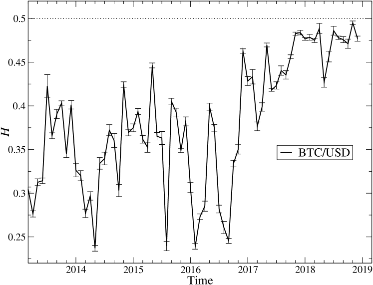
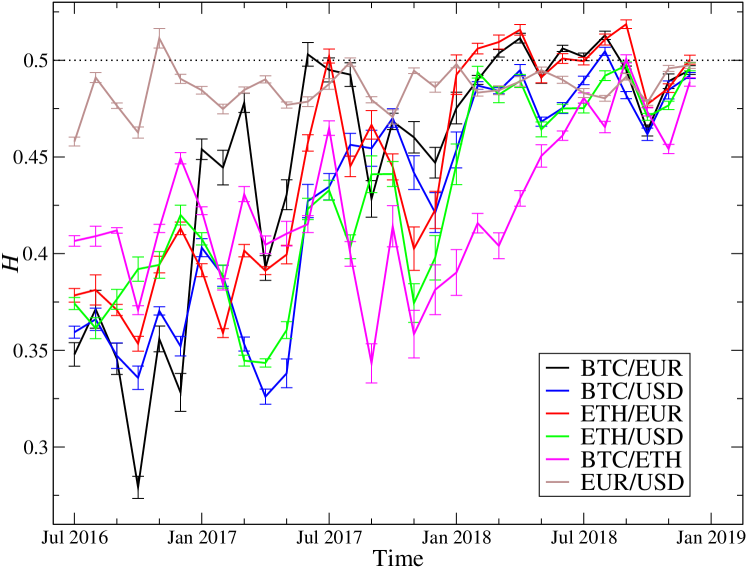
The Hurst exponent evolution for more exchange rates: BTC/EUR, BTC/USD, ETH/EUR, ETH/USD, and BTC/ETH can be shown based on data from the Kraken platform. This is done, however, in expense of a shorter interval available: July 2016–December 2018. The returns were constructed with s and was calculated over monthly windows – Fig. 22 (bottom panel). Like in the case of BTC/USD from Bitstamp, the exchange rates from Kraken were associated with until mid-2017. Then from 2018 the Hurst exponents increased to a 0.5 level for all the exchange rates involving USD and EUR, while BTC/ETH remained in the antipersistent regime until mid-2018. This shift of is parallel to the shortening of the inter-transaction times on Kraken that started in April 2017. For comparison, for the EUR/USD exchange rate is also shown – Fig. 22 (bottom panel). This demonstrates clearly the cryptocurrency market development [71].
| Name | Binance | Kraken |
| BTC/USD∗ | 0.47 | 0.48 |
| ETH/USD∗ | 0.48 | 0.49 |
| ETH/BTC | 0.51 | 0.48 |
| XRP/BTC | 0.46 | 0.45 |
| BCH/BTC | 0.48 | 0.43 |
| BCH/USD∗ | 0.48 | 0.48 |
| LTC/BTC | 0.47 | 0.45 |
| LTC/USD∗ | 0.47 | 0.47 |
| ETC/BTC | 0.47 | 0.45 |
| XMR/BTC | 0.46 | 0.43 |
| DASH/BTC | 0.46 | 0.44 |
| ETC/ETH | 0.42 | 0.41 |
| Average | 0.47 | 0.45 |
Table 2 shows values of the Hurst exponent calculated for the returns ( min) of a few equivalent exchange rates that were obtained independently from two platforms: Binance and Kraken. The time series cover the whole year 2018. On average, larger exponents can be observed for the cryptocurrency pairs listed on Binance, where is closer to . This goes in parallel with a higher trading frequency on this platform than on Kraken (see Sect. 3). The smallest Hurst exponent was obtained on both platforms for ETC/ETH, which is characterized by the lowest trading frequency correlating also with relatively small Hurst exponents for Kraken’s BCH/BTC, XMR/BTC, and DASH/BTC (in each case ).
4.3 Multiscaling of the exchange rates
The Hurst exponent discussed in the previous subsection can account for linear correlations only. A more subtle characteristics of the time series complexity is the occurrence of multiscale autocorrelations. They can be described by the generalized Hurst exponent family with that belongs to some predefined range related to the properties of the return PDF tails. can be calculated with help of MFDFA according to Eq.(9). A complementary information can be found in the singularity spectrum , whose width given by Eq.(11) can be considered as a measure of the time series complexity or diversity of its internal structure [114, 188, 117].
4.3.1 Temporal evolution of the multiscale autocorrelations
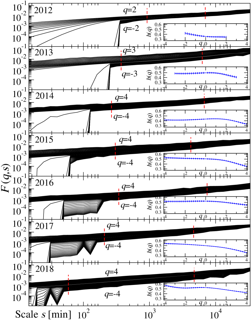
Figure 23 presents the fluctuation functions defined by Eq. 8 and the generalized Hurst exponents calculated for the s return time series of the BTC/USD exchange rate divided into annual intervals 2012-2018 (the Bitstamp data). A systematic improvement of the scaling quality can be observed each subsequent year, especially for (small returns). This improvement is closely related to the gradual shortening of the inter-transaction times on this exchange rate, thus shortening also the zero-return sequences that influence the algorithm output. In 2012 such intervals without trading reached 600 minutes, thus the range of satisfactory scaling is very short in this case. There was no dependence of on negative s until 2017 (see insets in Fig. 23). Thus, a power-law dependence of on during earlier years reflects solely the organization of the larger fluctuations. It can also be recalled that the CDF tail for BTC/USD increased from in 2012 to over 3 from 2014 on (Sect. 3). This result led to limiting the range in from [-2,2] for 2012, through [-3,3] for 2013, to [-4,4] for 2014 and the subsequent years (because of the non-existent higher-order moments of the corresponding PDFs).
Figure 24 presents the singularity spectra for the same individual years as Fig. 23. From 2013 until 2017 the spectra are asymmetric with strong dominance of the left wing corresponding to large returns and only in 2018 the right wing corresponding to small returns becomes significant. In the years 2013-2016 the asymmetry coefficient assumed values between 0.7 and 0.8. The spectrum was widest in 2017 attaining width with , while in 2018 it became symmetric with and . Based on these values, in 2018 can be categorized as multifractal with well-developed hierarchical organization for both the small and large returns. This means that, along with increasing transaction frequency on BTC/USD, the small returns ceased to behave like noise and the nonlinear correlations eventually built up also in this case. Such a symmetry between the fluctuations of different magnitude is a well-grounded observation on Forex [23, 189] and other mature markets [117, 98]. The results for 2012 and 2013 are characterized by the largest error, which is related to a short range of scaling in that may be used to assess the scaling exponents and . Moreover, taking into account the lack of long-range nonlinear correlations in 2012 (see Sect. 3.4), the time-series for this period can be considered as monofractal (if fractal at all).
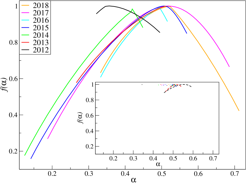
The observed multiscale characteristics disappear when considering the Fourier surrogates of the data [190] or the shuffled time series. In the former case, nonlinear correlations are destroyed through the Fourier-phase randomization of the original data and only linear correlations survive. Their singularity spectra are narrow and located at the values of that match the Hurst exponent of the original time series (see Fig. 24). In the latter case, shuffling destroys all correlations (i.e., linear and nonlinear) but preserves the return distributions. The spectra are also narrow and located roughly at . It should be pointed out that the slightly wider spectra featured for 2012 and 2013 are a numerical artifact caused by the heavy tails of the corresponding PDFs (see Refs. [114, 191, 121, 122] for more details).
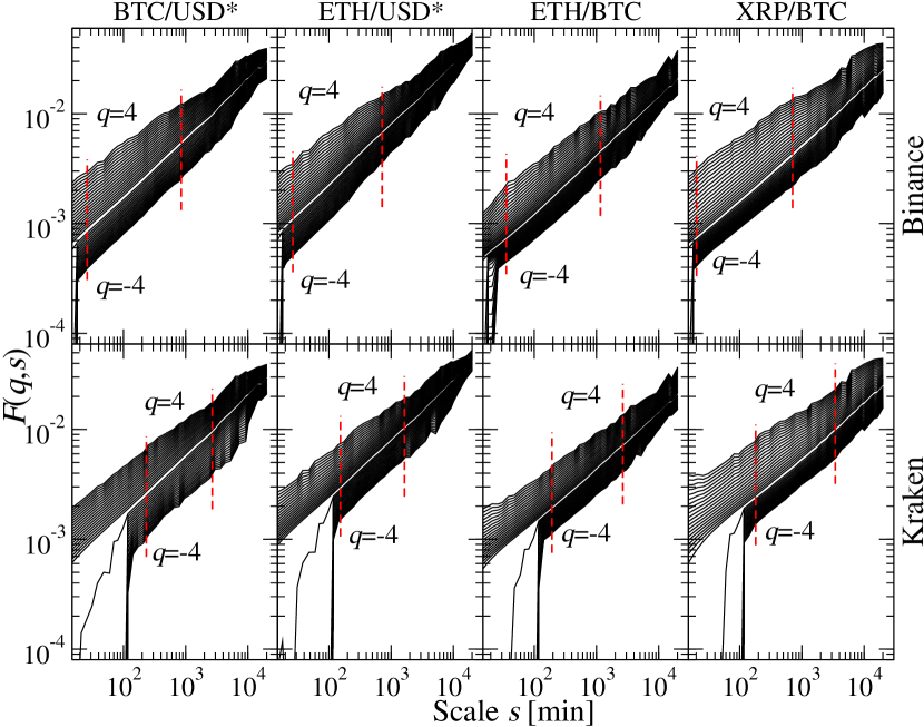
In order to look at a broader picture, one may also compare the multiscale properties of BTC/USD with other exchange rates or even the same exchange rates from different trading platforms. Fig. 25 exhibits the fluctuation functions calculated from the min returns of the most liquid exchange rates listed on Binance and Kraken: BTC/USD∗, ETH/USD∗, BTC/ETH, and XRP/BTC, where USD∗ means either US dollar (Kraken) or USDT (Binance). The data covers 2018. Since the related PDFs are heavy-tailed with , a range of was restricted to [-4,4] [192]. The functions are indefinite for small and negative because the considered exchange rates were traded with a moderate frequency, especially on Kraken, where non-trading intervals could be as long as 100 min. Fortunately, the scaling quality for min is comparable between both exchanges. The dotted lines in Figure 25 mark the range of scales , for which the singularity spectra presented in Fig. 26 were estimated. These spectra are characterized by a left-sided asymmetry on both platforms. For Binance they are slightly wider and more symmetric than for Kraken, which suggests that the nonlinear organization of the small fluctuations is better developed on the former platform, owing to a higher trading frequency there. Like in the case of BTC/USD from Bitstamp, the observed multiscale effects disappear here when the Fourier and the shuffled surrogates are considered. Other exchange rates listed in Tab. 1 (Sect. 3.4), which are quoted simultaneously on Binance and Kraken, cannot be compared between the two because of a low trading frequency on Kraken and the PDF heavy tails of the corresponding time series. However, in general the returns for these exchange rates are monofractal and they have already been characterized by the Hurst exponent (Tab. 2).
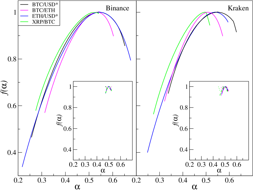
4.3.2 Multiscale characteristics for currencies and cryptocurrencies
Figure 27 shows and calculated or five the most liquid cryptocurrency pairs: BTC/EUR, BTC/USD, ETH/EUR, ETH/USD, and BTC/ETH from Kraken and, for a benchmark, the fiat currency pair EUR/USD from Forex. The returns with s cover an interval from July 2016 to December 2018. The scale range used to calculate is denoted by vertical dashed lines in each case. A maximum used to estimate should not be longer than the length of the average cluster of volatility assessed with the help of autocorrelation function (Sect. 3.4), otherwise the estimated is not credible [114]. Similar to BTC/US from Bitstamp discussed in Sect. 4.3.1, on Kraken the long periods without transactions lead to with undefined values for the negative s and for the small scales . This effect does not occur in the case of EUR/USD, because Forex is a much more liquid market.
A lack of dependence of on for the negative s and a clear dependence for (insets of Fig. 27) indicates that a heterogeneous hierarchical organization can only be seen for the medium and large returns, while the small returns are rather homogeneous. In contrast, for EUR/USD is symmetric, proving that the fluctuations of all magnitudes are responsible for the multiscale organization of the data. It appears noteworthy that a symmetric characterized also BTC/USD in 2018.
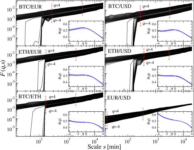
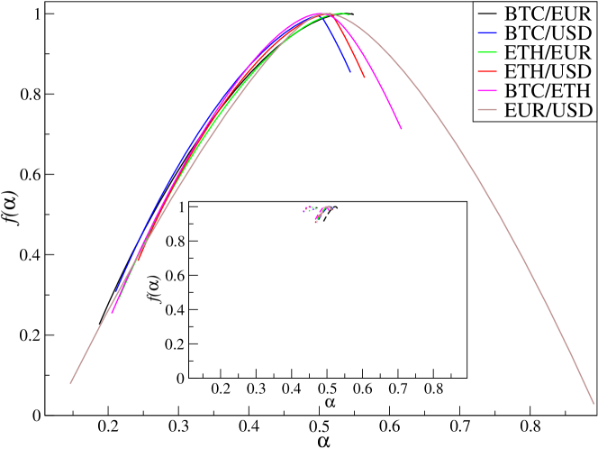
The multiscale properties characterizing the cryptocurrency exchange rates from Kraken and EUR/USD from Forex are illustrated in Figure 28, where their singularity spectra are compared. The spectrum for EUR/USD is the widest with and the most symmetric with . The widest spectrum for Kraken, representing the crypto-crypto pair BTC/ETH, is a result of the longest right-side wing of with . This spectrum is still considerably narrower if compared to that for EUR/USD, however. The other cryptocurrency/fiat exchange rates are also characterized by the left-sided asymmetry: and in each case. As a consequence, the small returns quantified by the right wing of behave as if they were monofractal noise. This results confirms that the Forex exchange rates show more complex dynamics than the cryptocurrency exchange rates.
The observed multiscale effects disappear entirely if the non-linear correlations are selectively destroyed via the Fourier surrogates or if the returns are shuffled. In the latter case, the impact of the heavy tails on the singularity spectra is evident (inset of Fig. 28). The spectra for the shuffled data are a little broader if compared to the case of the Fourier surrogates. However, they are narrower than their counterparts derived for BTC/USD from Bitstamp in 2012 and 2013, which stems from the thinner return PDF tails on Kraken.
Summing up, complexity of the BTC/USD exchange rate returns has evolved in time and, by 2017, it approached the complexity observed typically on Forex and even attained that level in 2018. Similar conclusion could be drawn for the exchange rates listed on Kraken, where ETH/USD shows the multiscale properties similar to BTC/USD. An exchange rate without any fiat currency involved – BTC/ETH – also reveals complexity typical for Forex. The exception that allows for distinguishing between the cryptocurrency exchange rates and the Forex ones is a less evident hierarchical organization of the small fluctuations in the former case. This is because a high trading frequency is needed to develop multiscaling at the level of small fluctuations. The impact of trading frequency is also seen when comparing the same exchange rates listed on different trading platforms. On Binance, where the frequency is larger, the return time-series show the multiscale properties that are closer to those typically observed on Forex than their counterparts listed on Kraken.
5 Multiscale cross-correlations
Throughout the two preceding sections, it was shown that the cryptocurrency exchange rate fluctuations are characterized by heavy tails of the return probability distributions and by volatility clustering related to nonlinear temporal correlations in the returns and responsible for multifractality. Additional properties are revealed when one considers multivariate data consisting of two or more exchange rates. In Sec. 5.1, cross-correlations among the cryptocurrencies and fiat currencies will be analyzed using the previously-presented methods based on detrending, namely the MFCCA (Sect. 4.1.1) and (4.1.2). These allow for a quantitative description of nonlinear cross-dependencies over different time-scales and fluctuation magnitudes, conferring a significant advantage over classical linear correlation [116]. As for linear cross-correlations, the multifractal characteristics of individual time-series does not imply that such the same are also multifractally cross-correlated. Multifractal cross-correlations of the triangular arbitrage opportunity data will be discussed in Sect. 5.2.3. The results reported in this section are based on three data sets:
-
1.
Kraken-2: BTC and ETH quotations expressed in USD and EUR taken from Kraken and covering from Jul. 2016 to Dec. 2018, transformed to return time-series with s,
-
2.
Kraken-11: Quotations of BCH, BTC, DASH, ETC, ETH, LTC, REP, USDT, XMR, XRP, ZEC expressed in USD and EUR, taken from Kraken and covering the interval Jan. 2018 to Dec. 2018, transformed to return time-series with min (here, only the most liquid pairs were considered), and
-
3.
Binance-12: Crypto-crypto exchange rates obtained from BAT, BCH, BNB, BTC, ETH, ICX, IOTA, LTC, LSK, NEO, USDT, XLM taken from Binance and covering the same interval, also transformed to return time-series with min.
See Appendix A for the full names and statistical properties of all cryptocurrencies considered in this section.
5.1 Multiscale cross-correlations for the BTC and ETH
The bivariate fluctuation functions calculated (Eq.(6)) for the exchange rates involving cryptocurrencies show scaling behaviour over a range of scales. Figure 29 (main panels) illustrates this observation by showing for ten pairs of the exchange rate return time-series, representing the most liquid cryptocurrencies BTC and ETH (the Kraken-2 dataset), ordered from top to bottom with decreasing scaling quality.
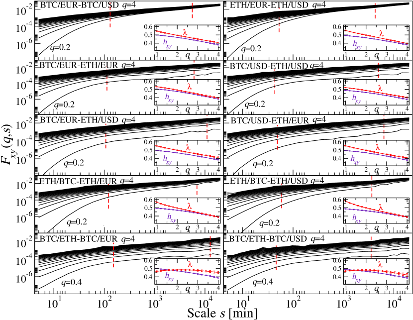
In this case, scaling signifies that the considered exchange rates are cross-correlated at various levels of their hierarchical organization. The most convincing scaling is seen for the bitcoin expressed in EUR and USD, as well as for the ethereum in the same fiat currencies (top panels). Contrariwise, the weakest scaling is associated with correlations for the exchange rates involving BTC and a fiat currency, or only cryptocurrencies, namely BTC/ETH (two bottom panels).
However, the scaling of can only be observed for medium and large returns () whereas, for small returns (), the function becomes negative and there is no multiscale cross-correlation. This finding agrees with the multifractal properties of the individual exchange rates reported in Sec.4, for which similar properties were also observed for medium and large returns, with their spectra accordingly featuring a strong left-side asymmetry. Indeed, this effect is typical for mature financial markets [189, 161, 58, 98].
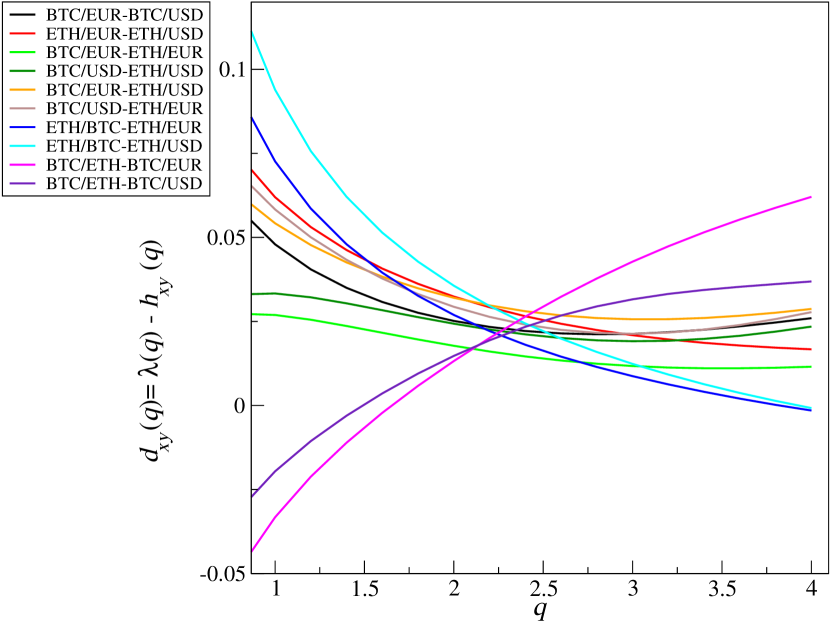
The dependencies of the scaling exponent and average generalized Hurst exponent defined, respectively, by Eq.(7) and Eq.(13) in Sect.4.1, are shown in Fig. 29. Through varying , reflects the multifractal character of cross-correlations between all 10 exchange rates, at least for . The weakest dependence on and, thus, the least-developed multifractality could be seen for BTC/ETH–BTC/EUR and BTC/ETH–BTC/USD, which are also characterized by the weakest scaling. The cross-correlations between these exchange rate pairs are also characterized by a negative difference ; this is in contrast with the other pairs, for which this is positive and depends appreciably on (Figure 30). The significant magnitude of observed for some exchange rate pairs implies a strong dependence of the cross-correlation on the scale (see Sect. 4.1.3). Indeed, since for the majority of pairs, the detrended cross-correlation coefficient increases substantially with for both medium and large returns, with this effect being stronger for than for (Figure 31). The same can be explained by the occurrence of large returns in the individual exchange rates, significantly contributing variance on small scales and counteracting the build-up of cross-correlations (i.e., on longer scales these are averaged out). Since for such returns are amplified more intensely than for , it becomes obvious that for small is closer to zero in the former case. However, this -dependence is less evident here than on mature financial markets [123, 161, 98], in particular the Forex, for which [58] (see Sect. 5.3 for further details).
The maximum level of depends on the exchange rate pair; for the dataset considered here, high values are attained by the pairs such that the same cryptocurrency is expressed in terms of the fiat currencies, USD and EUR, for which . This situation can be explained by the considerably lower volatility of EUR/USD as compared to the cryptocurrencies (Fig. 12). By contrast, the lowest level of is found for the pairs involving the same cryptocurrency expressed in a fiat currency and another cryptocurrency, namely BTC/ETH–BTC/EUR and BTC/ETH–BTC/USD. The remaining pairs are associated with intermediate levels of . Moreover, BTC/ETH–BTC/EUR and BTC/ETH–BTC/USD together with ETH/BTC–ETH/EUR and ETH/BTC–ETH/USD show a sign change of (Fig. 30) when transitioning from to , which hallmarks a change in the monotonic behaviour of for .
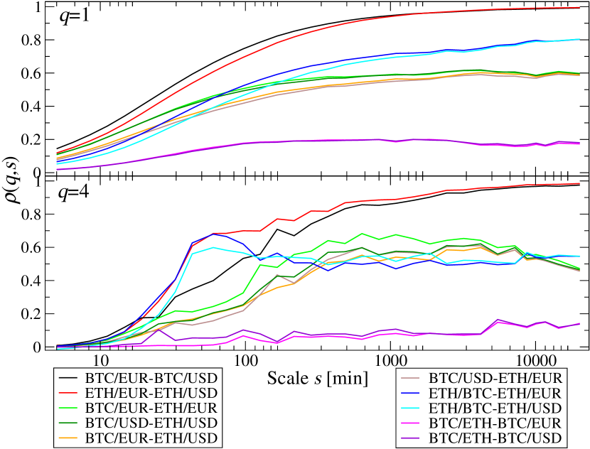
The Kraken-2 dataset covers the period Jul. 2016 through Dec. 2018, over which the cryptocurrency trading steadily accelerated, leading to a consistent reduction in the inter-transaction times. The coefficients calculated over a half-year periods are presented in Figure 32. During the interval from Jul. 2016 to Dec. 2017, the correlations on the smallest time-scales remained close to zero, and increased markedly with . This markedly changed during 2018, when became higher than before for small , and its maximum value was attained faster. The weakest correlations between BTC/ETH–BTC/EUR and BTC/ETH–BTC/USD observed in Fig. 31 can be accounted for the fact that, following the crash of the cryptocurrency market in Jan 2018, flipped sign because both the BTC and ETH decreased with respect to the EUR and USD (Fig. 13). However, the decrease observed for the ETH is larger and faster than for the BTC, so BTC/ETH rate can be seen to rise, weakening the global (i.e., whole-period) correlations between BTC/ETH and BTC/EUR, and between BTC/ETH and BTC/USD. For comparison, it should be noted that does not depend on in the case of a Forex exchange rate cross-correlation, such as EUR/USD–EUR/JPY (bottom right panel of Fig. 32), which is typical in low-volatility periods wherein no extraordinary event affects the Forex systematically [58].
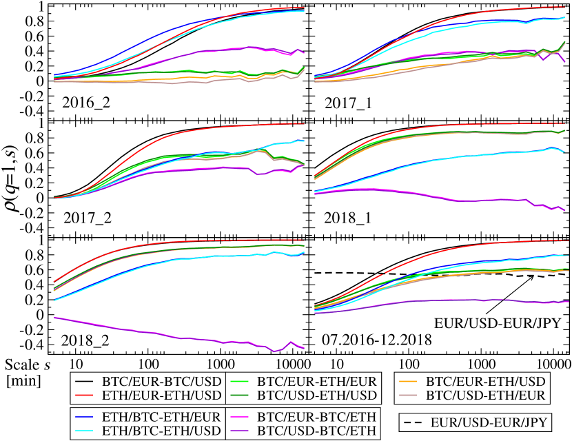
Until the end of 2017, insofar as two exchange rates hinged around a common base currency (e.g., BTC/EUR–ETH/EUR and BTC/USD–ETH/USD), one would observe a stronger cross-correlation compared to the situation of different base currencies (e.g., BTC/EUR–ETH/USD and BTC/USD–ETH/EUR); an example is visible in Fig. 32. In 2018, however, similar cross-correlation levels could already be seen between the two cases. This observation can be explained in terms of the market synchronization that takes place over longer time-scales; it is also related to a significant slowing in the frequency and size of the triangular arbitrage opportunities over the period from Mar. 2018 to Dec. 2018, as visible in Figure 33.
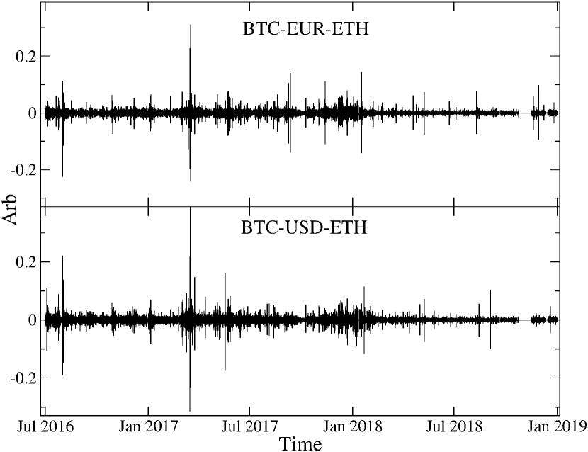
Three (crypto)currencies are deemed to be in a triangle relationship if it is possible to make a transaction cycle through three exchange rates and return to the initial (crypto)currency [57, 58]. Given the five exchange rates from Kraken-2, two triangles are available: EUR BTC ETH EUR and USD BTC ETH USD, where the double arrows indicate the two possible exchange directions [57]. The arbitrage opportunity occurs at a time if
| (19) |
or
| (20) |
The formulas are, evidently, unchanged when considering the USD in place of the EUR. Because the bid price for the same exchange rate needs to be lower than the ask price, such arbitrage opportunities are rather rare. For example, on Forex they occur only during events that elevate the volatility [58].
In the case of a dataset without the bid and ask prices, it is impossible to calculate the exact arbitrage opportunity as one has to replace the exchange rates in Eq.(19) and Eq.(20) with logarithmic prices at the end of each interval of length :
| (21) |
where A/B is the exchange rate between the (crypto)currencies A and B, and . For the above-mentioned triangles, the following arbitrage cases are possible:
| (22) |
| (23) |
If Arb(EUR-BTC-ETH) or Arb(USD-BTC-ETH) , there exists a possibility of carrying out the arbitrage. Time-series of the arbitrage opportunity are shown in Fig. 33. Towards the end of 2018, their frequency and size decreased, which could be associated with a more intense synchronization of the exchange rates engendered by the inter-transaction time shortening on Kraken. This situation also translates into an increased cross-correlation level over the shortest time-scales during the same period.
5.2 Multiscale cross-correlations on the different trading platforms
This section reports the primary results concerning the exchange-rate cross-correlations of liquid cryptocurrencies on the two trading platforms, Kraken (the Kraken-11 dataset) and Binance (the Binance-12 dataset). More specifically, both the cross-correlations within one platform and the inter-platform ones were considered. Only BTC and ETH (Kraken) and BTC, ETH, USDT, and BNB (Binance) were liquid enough to serve as bases. For each platform, a symmetric -correlation matrix , where , can be created for each scale , whose entries correspond to calculated for two exchange rates, with .
5.2.1 Intra-platform multiscale cross-correlations
The representative behavior of in four typical cases for each platform is shown in Fig. 34 (Kraken) and Fig. 35 (Binance).
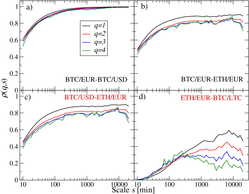
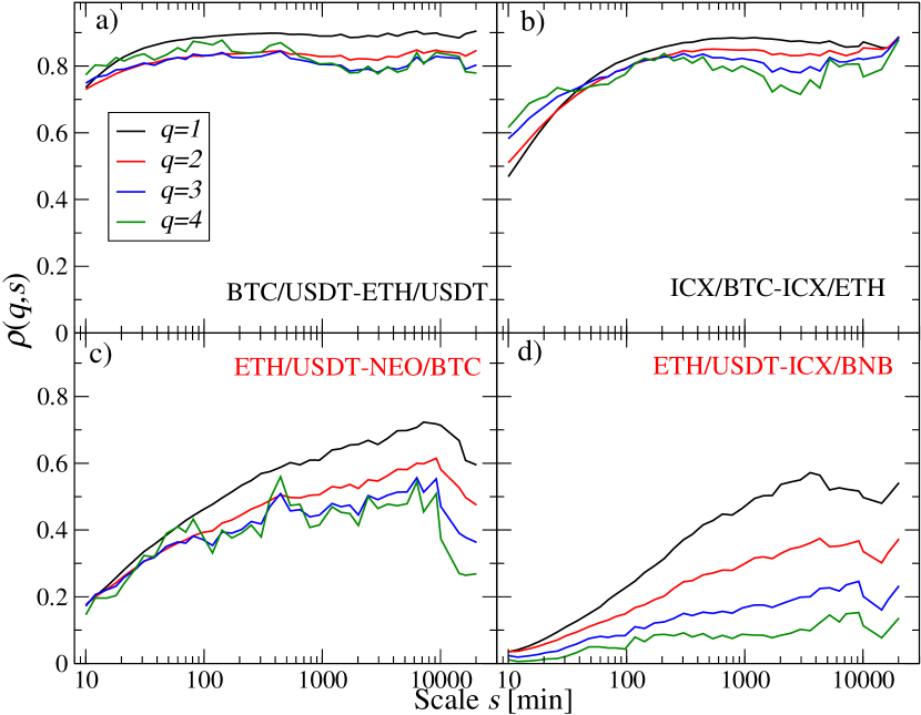
Among the exchange rates considered for Kraken, the strongest correlation, approaching unity for large , is seen for BTC/EUR–BTC/USD (Fig. 34(a)); this indicates that, on such scales, it is largely irrelevant whether the BTC is expressed in EUR or USD, since the traditional currencies are markedly less volatile than the cryptocurrencies. Over shorter scales, however, the cross-correlations are weaker for any setting of , because the market is incompletely synchronized and there occur arbitrage opportunities. Meanwhile, for a given , is larger for shorter average inter-transaction intervals. The cross-correlation strength for the cryptocurrencies expressed in the same fiat currency, EUR or USD, ranks second, with the largest value of ( min) observed for the most liquid pair, namely BTC and ETH (Fig. 34(b)).
The third case is a situation that characterizes Kraken in particular: a pair of exchange rates does not form a triangle relation (i.e., four (crypto)currencies are involved), but one cryptocurrency is expressed in USD whereas the other in EUR. If the cryptocurrencies are BTC and ETH (Fig. 34(c)), the cross-correlation strength is only slightly lower than that in Fig. 34(b), and it is only for the smallest . Again, this is connected to the small volatility of the fiat currencies. Finally, there is the case of exchange rates that also do not form a triangle, but involve only one fiat currency. Here, a maximum is considerably smaller than in the previous cases; the most strongly correlated pair is ETH/EUR–BTC/LTC, with and even for the longest scales (Fig. 34(d)). For the shortest scales considered ( min), such exchange rates are largely independent of each other. A notable feature is the significant dependence of the cross-correlation strength on .
Since on Binance cryptocurrencies are only traded among themselves, one cannot calculate for BTC/X–BTC/Y, where X, Y are fiat currencies, and one cannot create a plot equivalent to Fig. 34(a). Nevertheless, it is possible to use Tether (USDT) as a proxy for the US dollar, and thus create a plot equivalent to Fig. 34(b). Indeed, Fig. 35(a) shows that the cross-correlation between the exchange rates that involve the same “fiat” base, i.e., BTC/USDT–ETH/USDT, is the strongest among all the rates considered on Binance. By replacing the USDT with ICX, a less liquid cryptocurrency, the cross-correlations decrease for small , while remaining on a level similar to that for USDT for min (Fig. 35(b)).
If the exchange rates do not share the same base, they do not form a triangle, and is substantially smaller than in panels (a) and (b) over all and all scales (Fig. 35(c)-(d)). Since, over small , trading on different exchange rates does not happen to be synchronized, especially for the exchange rates that do not form any triangle (no arbitrage possibility), the cross-correlations are much weaker than over large , from the perspective of which trading is more synchronous. The liquidity of a cryptocurrency liquidity plays a key role here: for the more liquid exchange rates, e.g., BTC/NEO in Fig. 35(c), the maximum level of is higher compared to the less liquid ones, e.g., ICX/BNB in Fig. 35(d).
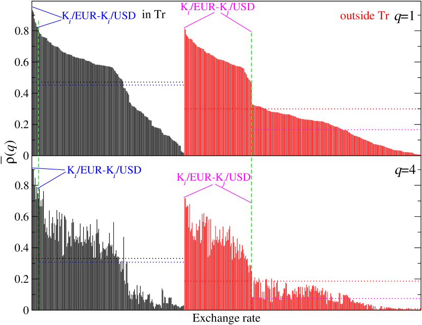
Cross-correlations between the exchange rates of the form Ki/EUR–Kj/USD, where Ki, Kj () denote cryptocurrencies, are on average stronger than those involving only a single fiat currency X, i.e., Ki/X–Kj/Kl, or no fiat currency at all, i.e., Ki/Kl–Kj/Km, where . This is shown in Fig. 36 for all possible exchange rate pairs from Kraken-11, split into the triangle-related (black) and triangle-unrelated (red) ones. Each vertical bar represents the absolute detrended cross-correlation coefficient averaged over all scales: , and in descending order. By comparing the triangle cross-correlations with the non-triangle ones, it becomes apparent that a primary factor responsible for the magnitude of is the number of exchange rates that revolve around a fiat currency: the exchange rates of two cryptocurrencies tend to be less correlated with the other exchange rates than those involving the USD or EUR. Notably, this property is largely preserved if a different value of is selected (e.g., compare the top and bottom panels of Fig. 36).
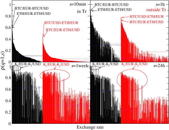
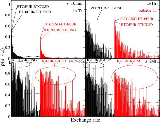
Fig. 37 shows calculated for representative individual scales (i.e., min, h, day, and days) instead of , and arranged in the same manner as Fig. 36, for (top panel) and (bottom panel). Typically, the magnitude of increases with raising for a given exchange rate pair with the largest cross-correlation, close to unity, being reached for Ki/EUR–Ki/USD in accordance with Fig. 34(a). Thus, on long temporal scales, it becomes inconsequential whether a cryptocurrency is expressed in EUR or USD. This effect is visible not only for the most liquid cryptocurrencies, e.g., the BTC and ETH, but also for the less liquid ones. However, for min, only the most liquid exchange rates feature . By increasing and focusing on the larger returns, one observes that only the exchange rates having the form Ki/EUR–Kj/USD differ from 0 significantly on the shortest scale min; these exchange rates also increase most markedly in .
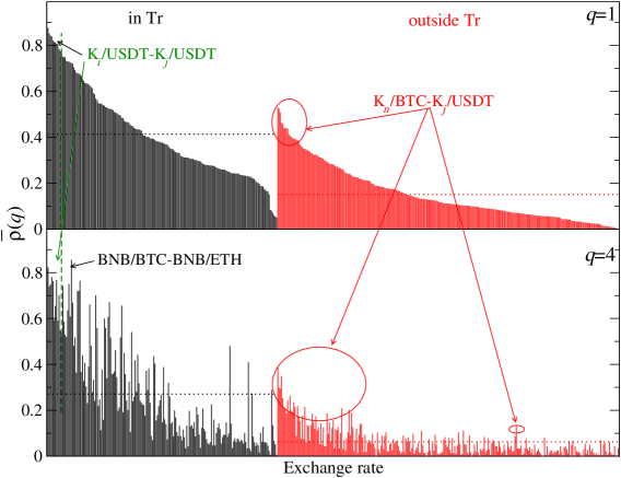
The same key factor, namely the average number of transactions in a time interval, determines the cross-correlation strength on the Binance platform (the Binance-12 dataset). Given the absence of any exchange rate involving fiat currency, for the strongest cross-correlations are those observed for the exchange rate pairs involving two different cryptocurrencies alongside a common base, USDT: Ki/USDT–Kj/USDT (the triangle-relation case with Ki, Kj=BCH, BNB, BTC, ETH, LTC, NEO, K Kj), and those involving two cryptocurrencies, USDT and the most liquid BTC: Kl/BTC–Kj/USDT (the non-triangle-relation case with Kl=BAT, BCH, BNB, ETH, ICX, IOTA, LTC, LSK, NEO, XLM, K Kj); see Fig. 38. However, the agreement between the magnitude of for and is less clear on Binance than on Kraken, because of higher volatility of the cryptocurrencies as compared to USD and EUR.
On the level of individual scales, the average cross-correlations among the Binance exchange rates increase with (see Fig. 39), which is in agreement with Fig. 35 and points to the analogous result obtained for the Kraken data (Fig. 36). In contrast with Kraken, however, the largest values of do not change with in the case of the triangle-forming exchange rates Ki/USDT–Kj/USDT (for ) and BTC/Km–ETH/Km, where Ki and Kj denote the same cryptocurrencies as in the preceding paragraph, and Km denotes any cryptocurrency denoted by Kl and additionally USDT (for ). On the other hand, the pairs Kl/BTC–Kj/USDT are the strongest cross-correlated ones among the triangle-unrelated exchange rates. On Binance, there is a considerably larger difference in between the triangle-related and the triangle-unrelated rates on the short scale of min. In the former case (i.e., with a common base cryptocurrency), market synchronization occurs on shorter scales because of the triangular arbitrage possibility. In contrast, in the latter case (i.e., lack of a common base), there is no direct arbitrage possible, and a longer time is needed to synchronize the exchange rates.
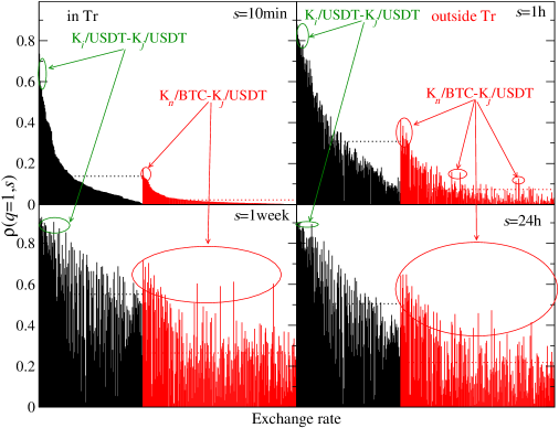
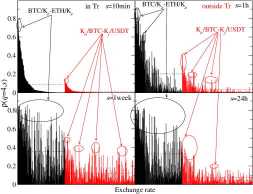
Remarkably, since the cross-correlations among the exchange rates differ in magnitude, a cross-correlation hierarchy is formed, which can be expressed as a dendrogram by applying a hierarchical clustering algorithm [7, 22, 193]. As this is defined over a metric space, each average -coefficient for the exchange rates and must be transformed to a respective distance , defined as follows
| (24) |
where the absolute value is taken to eliminate the impact of exchange direction. This definition of implies that with for perfect cross-correlation between the exchange rates and , and for statistically independent pairs.
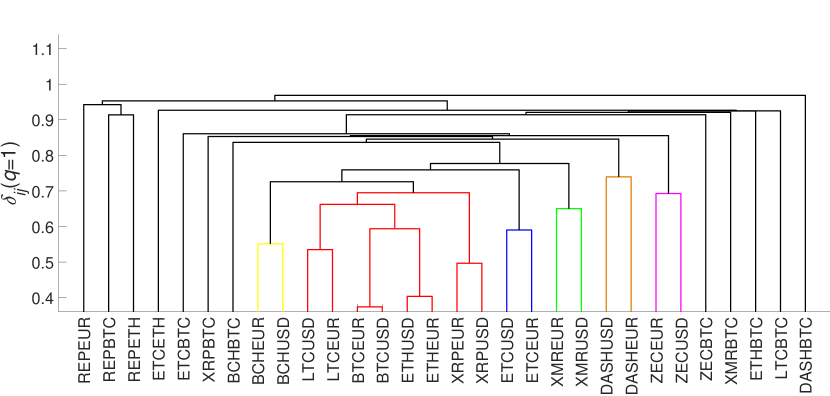
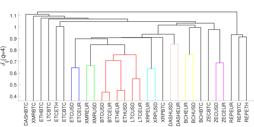
The so-constructed dendrograms are presented in Fig. 40 for the exchange rates from Kraken (except for USDT/USD, which is independent of the rest of the market), and in Fig. 41 for the exchange rates from Binance (except for the least correlated one, LSK/BNB). On both platforms, the distances increase with (i.e., substantial returns are less cross-correlated than typical ones) but, for a given , they are typically larger on Binance; actually, this could already be observed in Fig. 36 and Fig. 38 based on . On Kraken, clusters for and appear similar to each other, with the most liquid cryptocurrencies (i.e., BTC, ETH, LTC, and XRP) being separated the least if expressed in fiat currencies (the red cluster). The other exchange rates form clusters insofar as the same cryptocurrency is expressed in EUR and USD; hence, they essentially elucidate a correlated movement of USD and EUR viewed from a perspective of less liquid cryptocurrencies.
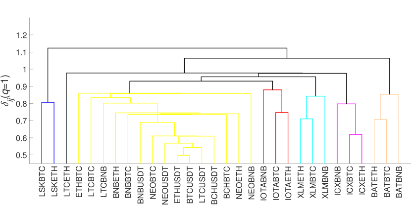
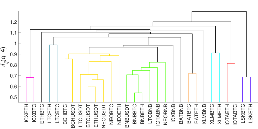
On Binance, two large clusters, based on USDT and BNB, can be distinguished for . On the other hand, a cluster of cryptocurrencies expressed in BNB does not exist for , and the exchange rates involving USDT merge with those involving the BTC, BNB, and ETH, as well as a few other rates, including BNB/USDT and NEO/BTC. Less liquid cryptocurrencies, such as LSK, ICX, BAT, XLM, and IOTA expressed in BTC, BNB, and ETH, form their own clusters. This arrangement signifies that, while the most liquid cryptocurrencies are strongly correlated within their group, the less liquid ones are more independent. For , the main clustering factor is a common base. A significant fluctuation of the base cryptocurrency price implies that all other assets become correlated if they are expressed in this particular cryptocurrency. This effect is also observed on the Forex when some currency experiences a high volatility period (see Ref. [58] for examples about the Swiss franc during the Swiss National Bank interventions in 2011 and 2015 British pound after the Brexit referendum result was announced in 2016).
5.2.2 Inter-platform multiscale cross-correlations
In this subsection, cross-correlations for the selected exchange rate pairs listed simultaneously on both Kraken and Binance are directly compared. In this context, the USD and USDT are treated as the same currency and denoted by USD∗.
Figure 42 shows the bivariate fluctuation function for the most correlated exchange rates in a triangle relationship, namely the BTC/USD∗–ETH/USD∗ (top panel), and without a triangle relationship, namely the ETH/USD∗–XRP/BTC (bottom panel). As in Sect. 5.1, is also presented here only for , and shows a consistent power-law dependence on scale. By contrast, for negative corresponding to small returns, fluctuates around zero, denoting the absence of cross-correlation among such returns (not shown because of the log-log plot). A difference between the platforms can be appreciated in insets of Figure 42, which present and as defined by Eq.(7) and Eq.(13) in Sect. 4.1. The difference between these quantities is considerably larger on Kraken than on Binance, which suggests that, on the latter, the exchange rates synchronize over shorter time-scales. Nevertheless, on both platforms the exchange rates without a triangle relation show a later synchronization onset (larger ) compared to the exchange rates in a triangle relationship, especially for .
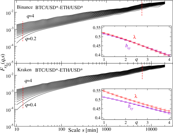
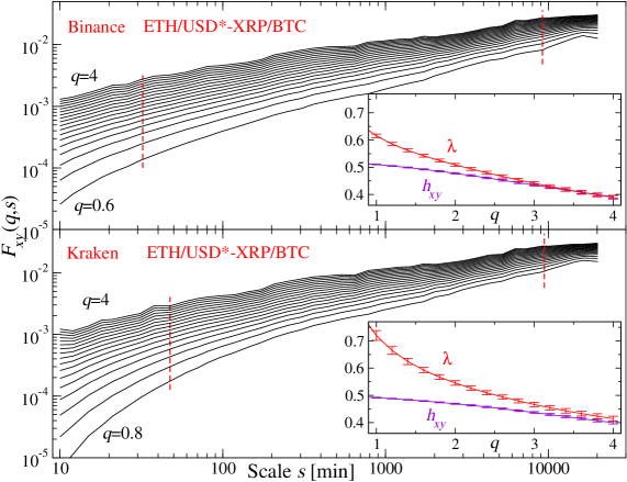
Given that corresponds directly to the functional behavior of , this quantity is shown in Fig. 43 for the same exchange rate pairs as in Fig. 42. Over the shortest scales, on the order of min, and for both BTC/USD∗–ETH/USD∗ and ETH/USD∗–XRP/BTC, is smaller in the case of Kraken: for ETH/USD∗–XRP/BTC, the cross-correlation even approaches zero. Moreover, substantially increases with (however, only in terms of its overall behavior, as is not sensitive to scale) on Kraken, which corresponds to positive (insets in Fig. 42). Differently, practically does not depend on for BTC/USD∗–ETH/USD∗ on Binance, which goes in parallel with in this case. On the other hand, in the case of the exchange rates that do not form a triangle (ETH/USDT–XRP/BTC) on Binance, for , which agrees with a weak average dependence of on in Fig. 43. The correlation strength on both platforms converges to a common level at the scale min, which defines the time needed to attain full synchronization of different exchange rates.
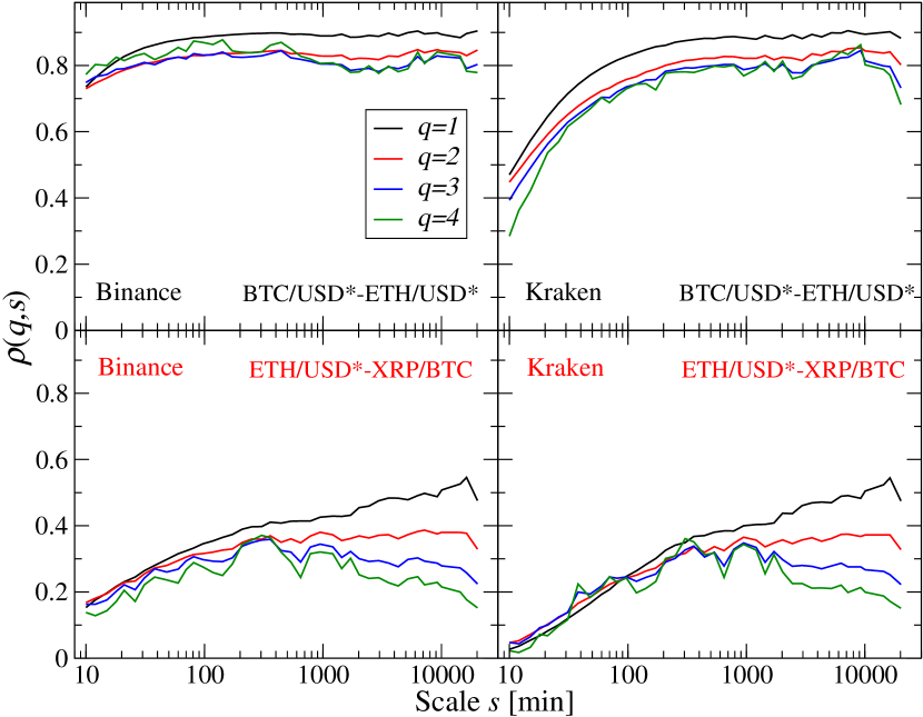
| Time scale | Binance | Kraken | Binance | Kraken | |
| Tr =10min | 0.163 | 0.092 | 0.117 | 0.029 | |
| P =10min | 0.045 | 0.029 | 0.021 | 0.005 | |
| Tr =1h | 0.309 | 0.229 | 0.208 | 0.162 | |
| P =1h | 0.120 | 0.086 | 0.061 | 0.070 | |
| Tr =24h | 0.490 | 0.479 | 0.262 | 0.259 | |
| P =24h | 0.299 | 0.287 | 0.120 | 0.123 | |
| Tr =1 week | 0.573 | 0.570 | 0.276 | 0.276 | |
| P =1 week | 0.381 | 0.380 | 0.139 | 0.137 | |
Table 3 presents averaged over all possible exchange rate pairs listed on both platforms for sample values of and . In almost every case, the triangle-related pairs produce larger than the unrelated ones. While for shorter time-scales (i.e., min and hour) the cross-correlations are stronger on Binance than Kraken, for longer time-scales (i.e., day and week) the correlation levels converge, as was already been pointed out above (Fig. 43).
Since there are exchange rates listed on both platforms, pairs may be formed not only within the same platform but also across them, for example, drawing the first from Binance and the second from Kraken. As events on Binance may occur ahead of Kraken or vice versa, an additional parameter has to be introduced, namely a delay , whose sign denotes which exchange rate is delayed: here, signifies that an exchange rate representing Binance leads, whereas means this exchange rate is lagged with respect to Kraken. Figure 44 displays the fluctuation function for a sample exchange rate involving the most liquid cryptocurrencies BTC/ETH. Different temporal relations between the time-series are considered: (top), min (middle), and min (bottom). The scaling quality of is maximized and the difference is minimized if Binance leads by a minute (middle panel). The weakest scaling and the largest can be seen in the opposite case when Kraken leads by a minute (bottom panel). The equal-time case () is located in between these extremes.
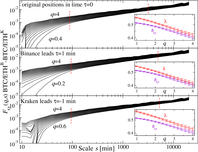
The cross-correlation strength for the pair BTC/ETH–BTC/ETH, expressed in terms of for min, min, and min, is shown in Fig. 45 (left). While, for all considered lags , the function converges to unity over sufficiently long scale , which is a desired effect in the case of the equivalent exchange rates, the strongest cross-correlation at the shortest scales of min is observed for min and min. This finding implies that the BTC/ETH movements on Binance are, on average, advanced by 1-2 min with respect to Kraken. For , the cross-correlation is weaker as well as for and min. This picture is stable across different positive values of (top left and bottom left), suggesting that the effect is present on both typical and large returns. A leading position of Binance is by no means surprising, as the BTC/ETH volume traded and associated trading frequency are higher than on Kraken. These results, based on , are supported by the characteristics of , which is the smallest for min and min, as visible in Fig. 45 (right).
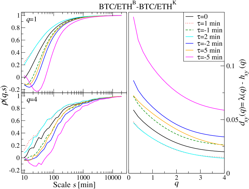
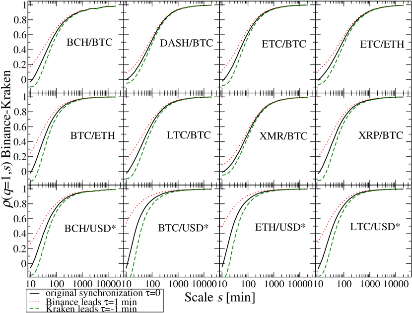
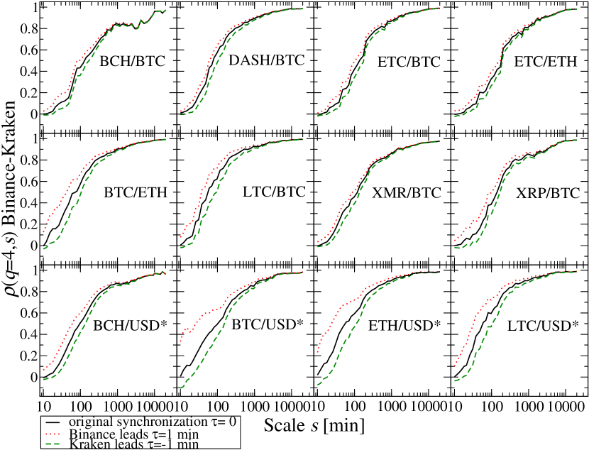
The leading role of Binance is also visible for the remaining 11 cross-platform exchange rate pairs by means of calculated for min, , and min (Fig. 46). While, in each case with , Binance is advanced by 1 min (the largest value of ), the exact cross-correlation strength depends on the exchange rate liquidity, with the most liquid rates being BTC/USD∗ and ETH/USD∗. Like for BTC/ETH, the cross-correlation strength increases with and converges to unity, more slowly for than for . Furthermore, for (large returns), not all exchange rates synchronize more markedly when min is used; in this regard, it is possible that, for the less liquid exchange rates, the market needs a longer lag to sense synchronization of large fluctuations. This effect could be accounted for by the higher trading frequency on Binance. In other words, when a transaction is completed on it, and there is no parallel trade on Kraken, the next transaction on Kraken will take into account what already has happened on Binance.
Another platform specialized in cryptocurrency trading is Bitstamp. The detrended cross-correlation coefficient calculated from the BTC/USD∗ returns (USD∗ stands for USD on Bitstamp) with min traded simultaneously on two out of three platforms: Binance, Kraken, and Bitstamp, is plotted in Fig. 47 for data spanning the entire year 2018. For Bitstamp vs. Kraken data, the effect of the asymmetric information spreading is absent, and for any , the cross-correlations are strongest for . On the other hand, comparing Binance and Bitstamp data, the situation resembles that of Binance vs. Kraken, i.e., Binance advances by 1 min. This can be explained in terms of the trading frequency, which is comparable between Bitstamp and Kraken, but lower than on Binance.
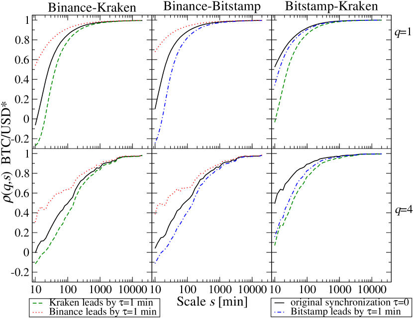
5.2.3 Arbitrage on the cryptocurrency market
Exchange rates on the Binance platform are characterized by higher volume and trading frequency compared to their counterparts on Kraken (see Tab. 1) in Sect. 3.3. Due to the less frequent trade, information needs more time to diffuse, directly translating into triangular arbitrage opportunities. In an analogy with Eq.(23), these are defined as an exchange rate return sum
| (25) |
where is calculated according to Eq.(21) and A, B, C are cryptocurrencies (in the case of Kraken, additionally including the USD). Time-series of the arbitrage opportunities at the return time sampling frequency min on Binance and Kraken (independently) for BTC/USD∗, BTC/ETH, and ETH/USD∗ are presented in Fig. 48. The largest arbitrage opportunities occurred in parallel on both exchanges at the beginning of 2018, i.e., during a period of highest volatility, which accompanied the cryptocurrency market crash. Their magnitudes, however, were systematically larger on Kraken.
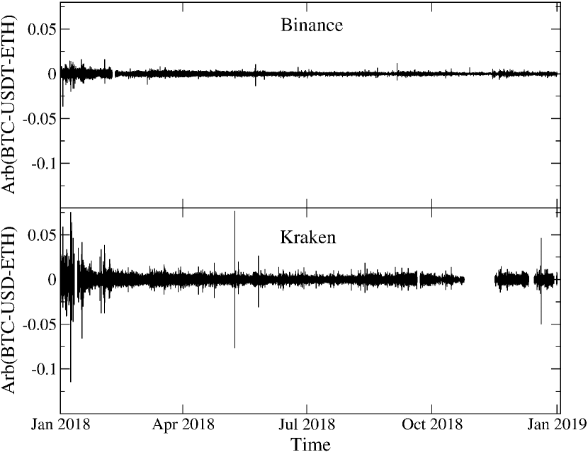
Tab. 4 lists the average and the maximum Arb values of the arbitrage opportunity for all triangles that can be created simultaneously on both platforms based on the available data (the Kraken-11 and Binance-12 datasets). Both and Arb are markedly lower on Binance. The smallest values of these quantities occur for a triangle including the most-traded exchange rates, namely, the BTC/USD∗, BTC/ETH, and ETH/USD∗. Triangular arbitrage opportunities for the exchange rates listed separately on Binance and Kraken are provided in the Appendix A in Tables 8 and 9.
| Kraken | Binance | |||
|---|---|---|---|---|
| Triangle | Average | Max | Average | Max |
| BTC-USD∗-ETH | 0.0017 | 0.1147 | 0.0006 | 0.0367 |
| BTC-USD∗-BCH | 0.0028 | 0.4701 | 0.003 | 0.0793 |
| BTC-USD∗-LTC | 0.0019 | 0.2016 | 0.0009 | 0.093 |
| ETC-ETH-BTC | 0.0019 | 0.246 | 0.0014 | 0.063 |
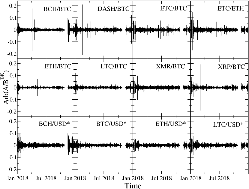
The leading role of Binance results in the cross-platform correlations that was discussed in Sect. 5.2.2, and is also identifiable in the arbitrage opportunity data comprising 12 exchange rates listed simultaneously on it and Kraken. In this context, time-series are defined by
| (26) |
where is given by Eq.(21), B stands for Binance, and K for Kraken. As expected, the largest opportunities occur on the least liquid rates, namely, DASH/BTC, ETC/BTC, and ETC/ETH (Fig. 49). Conversely, on the most liquid rates such as BTC/USD∗, ETH/USD∗, and BTC/ETH, arbitrage is a rare event at the sampling frequency of min, and its magnitude is considerably lower.
It appears as though the effect of the synchronization delays experienced by the different trading platforms occurs over time-scales that are unique for the cryptocurrency market and vastly longer than the other markets, like the Forex or the stock market. This is due to the decentralization, slower information spreading, and lower liquidity of the cryptocurrency market. It translates into numerous arbitrage opportunities, both for exchange rate pairs and triangles. Also, there is no reference price of a cryptocurrency, unlike in the Forex where Reuters offers the reference rates. Similar effects were analyzed by applying the same methodology to the stock markets [130] and oil markets [98], but the results were not as conclusive as for the cryptocurrency market.
To summarize this part, it can be stated that (1) the more frequently traded cryptocurrencies are, the faster is the synchronization of their fluctuations. This leads to high cross-correlation values over short time-scales and their weak dependence on , which translates into a small difference in . (2) The cross-correlations between the exchange rates forming a triangle are more robust, especially over time-scales on the order of a minute, compared to those not related in this way. (3) Large fluctuations are more weakly cross-correlated than medium ones. However, this difference is smaller than in the Forex, which will be addressed in Sect. 5.3. (4) The arbitrage opportunities in a triangle relationship are sparser on the frequently-traded exchange rates, and their magnitude is smaller.
5.3 Multiscale cross-correlations and triangular arbitrage on Forex
The Forex differs from the cryptocurrency markets in the volume traded, transaction frequency, liquidity, and factors related to its external connections with economy and politics. Predictably, its multiscale properties are therefore different. To illustrate this, a selection of the eight most liquid major currencies are considered in this section, namely the Australian dollar (AUD), Canadian dollar (CAD), Swiss franc (CHF), Euro (EUR), British pound (GBP), Japanese yen (JPY), New Zealand dollar (NZD), and US dollar (USD). Each currency can be expressed in the remaining ones, giving a total of 28 exchange rates (all of them are explicitly listed in Figure 50). The representative data were drawn from the Forex broker Dukascopy [93], and cover the year 2018.
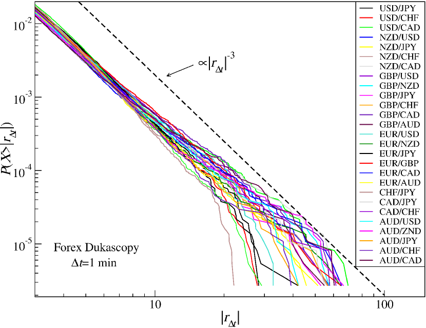
As for the cryptocurrencies, the returns are calculated with min. For most of the exchange rates, the inverse cubic law is met by the return CDFs when (Fig. 50). Therefore, the bivariate fluctuation function may be calculated for without concerns about moment divergence.
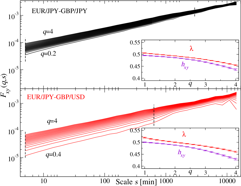
The bivariate fluctuation function reveals better scaling for the triangle-related exchange rates (i.e., a common base currency, top panel), which translates into a smaller distance between and compared to the exchange rates without a triangle relation; Fig. 51 illustrates this based on two sample cases (i.e., a triangle relation - top, without triangle - bottom). In both cases, the difference is maximal for , unlike the cryptocurrencies, for which the largest arises for (Fig. 30). In general, this difference is smaller on the Forex than the cryptocurrency markets, since the cross-correlation strength depends less markedly on (Fig. 52). This effect can be attributed to the larger liquidity of the Forex exchange rates because, on the cryptocurrency platforms, does not depend on the scale for the most liquid pair, BTC and ETH, expressed in a common base currency. The most pronounced difference between cryptocurrencies and fiat currencies is the much higher values of for the Forex exchange rates without a triangle relationship. In the case of cryptocurrencies, approaches zero on the shortest scales for the out-of-a-triangle rates. On the Forex, is also lower in this case than for triangle-related exchange rates (Fig 52), but not as substantially as in the cryptocurrency market. Large returns are, in general, considerably less cross-correlated on the Forex than on the cryptocurrency market: namely, there is a substantial dependence of on for both the in-triangle and out-of-triangle exchange rates (Fig. 52).
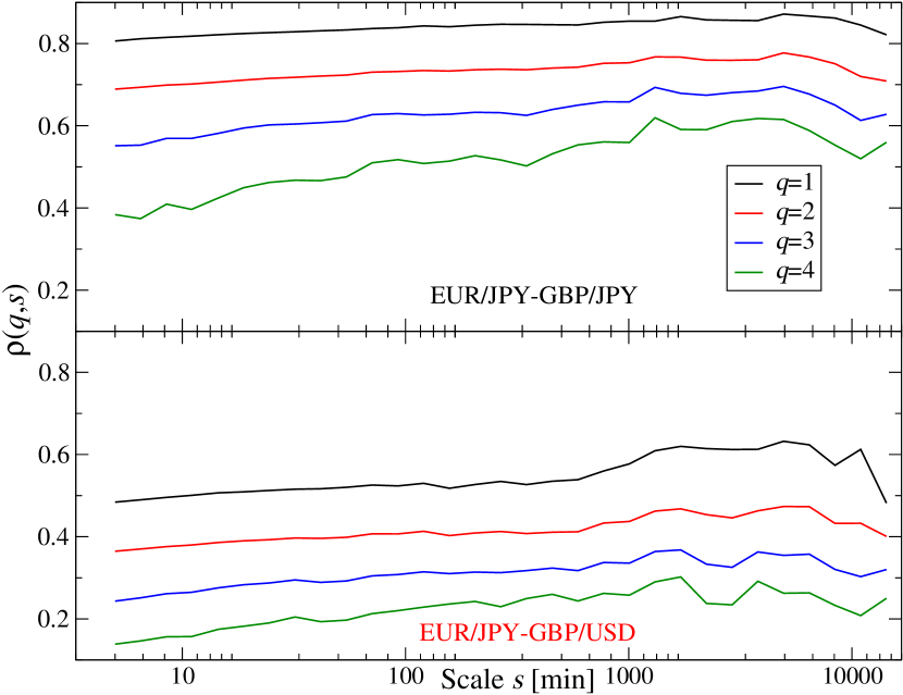
Fig. 53 shows for all exchange rates under consideration over four scales, namely min, h, day, and week. For , the coefficient only weakly depends on scale, while such a dependence is more pronounced for . The exchange rates in a triangle relation are considerably more strongly cross-correlated than those not related in this way (black vs. red plots). Since the AUD and NZD represent countries whose economies are greatly coupled, the exchange rate pairs of the form Wi/AUD–Wj/NZD, where Wi, Wj denote all the other currencies, behave effectively as if Wi and Wj were expressed in a common base currency, which significantly amplifies the corresponding .
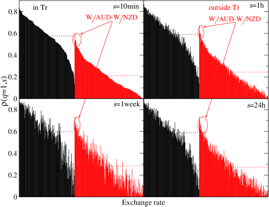
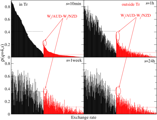
For , there is a large difference in the cross-correlation strength between the in-triangle and the outside-triangle exchange rate pairs, at both the individual and average levels; is also smaller than for . Furthermore, a moderate scale dependence can be appreciated for the outside-of-triangle exchange rates. The shifts in the ranked positions of with increasing are substantial, but this does not lead to an increase in the average cross-correlation levels (horizontal lines in Fig. 53), unlike the cryptocurrencies showing for min (see Fig. 37 and Fig. 39 in Sect. 5.2.1). A difference in trading frequency between the cryptocurrencies and the fiat currencies can plausibly account for this observation.
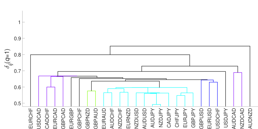
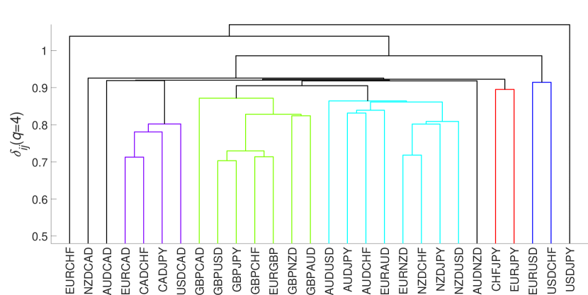
A cross-correlation hierarchy of the 28 exchange rates calculated with the hierarchical clustering algorithm from shows that the large fluctuation cross-correlations () form more pronounced clusters consisting of the exchange rates involving a common base currency, namely CAD, GBP, AUD, and NZD (Fig. 54). This arises because each independent movement of a base currency with respect to the other currencies contributes to their evolution, which can be viewed as their cross-correlation insofar as they are expressed in this particular base currency. The effect is most influential during the extreme volatility periods that typically accompany important economic and political events [58]. For typical fluctuations (), the subdivision into clusters is weaker. The most numerous cluster encompasses exchange rates not related by a triangle relation, namely, EUR/AUD–NZD/CHF and AUD/JPY–NZD/USD. This indicates that, for a sampling interval of min, the Forex is largely synchronized, and information is transmitted quickly, even outside triangle relations.
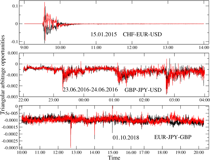
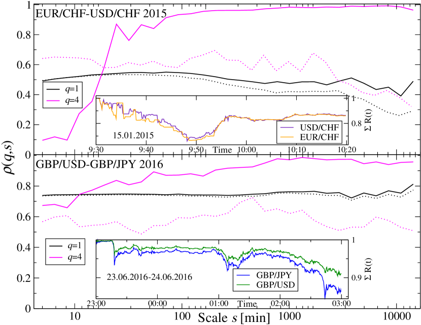
Together with the higher cross-correlation levels over the shortest scales , this is associated with a higher liquidity and trading frequency on the Forex. An associated effect is a much rarer occurrence of the triangular arbitrage opportunities. In Fig. 55, deviations from a triangle relation calculated for the bid and ask prices in analogy to Eq.(19) and Eq.(20) are shown for three triangles: CHF-EUR-USD, GBP-JPY-USD, and EUR-JPY-GBP during time-intervals of particular market instability, namely, stemming from the Swiss National Bank’s policy change on EUR/CHF, and the Brexit referendum (on the Forex, an arbitrage opportunity can occur only during elevated volatility periods [58]). Periods of maximum volatility are presented in detail in Fig. 56 (insets). During them, the individual exchange rates involving the CHF and GBP changed so rapidly that the others could not keep up, allowing the formation of arbitrage possibilities on the triangle-related exchange rates. For comparison, a day without any volatility-amplifying event from 2018 is also shown in Fig. 55. The main plots in Fig. 56 display calculated for the above-mentioned exchange rate pairs with and . The latter case shows that large returns during the turmoil periods are responsible for significant decorrelation of the exchange rates, whereas the average returns remain cross-correlated as customary. If these periods are removed, the arbitrage opportunities disappear, and the cross-correlation strength increases.
These properties of the Forex, including the paucity of arbitrage opportunities, more frequent trading, and shorter time-scales at which market synchronization occurs, motivate the view that the cryptocurrency market remains a markedly less mature market by comparison. Among the cryptocurrencies, only the BTC and ETH, when expressed in USD (or its equivalent USDT) on the most significant trading platforms, reveal signatures similar to those typical of exchange rates on the Forex.
5.4 COVID-19 impact on multiscale cross-correlations between the cryptocurrency market and traditional markets
Till beginning of 2020, it was generally believed that, viewed by many as a ”safe haven”, the cryptocurrency market was rather detached from the other financial markets and exhibited its individual dynamics [83, 86, 87, 88, 89, 90]. Whether this is still a valid hypothesis can be verified by calculating the generalized detrended cross-correlation coefficient given by Eq.(15) for time series of 1-min log-returns of BTC/USD and ETH/USD and 20 conventional assets, among which are 13 traditional currencies: Australian dollar (AUD), euro (EUR), British pound (GBP), New Zealand dollar (NZD), Canadian dollar (CAD), Swiss franc (CHF), Chinese offshore yuan (CNH), Japanese yen (JPY), Mexican peso (MXN), Norwegian krone (NOK), Polish zloty (PLN), Turkish lira (TRY), and South African rand (ZAR), 3 stock market indices: Dow Jones Industrial Average (DJIA), NASDAQ100, S&P500, and 4 commodities: gold (XAU), crude oil (CL), silver (XAG), and copper (HG), all expressed in US dollar. Fig. 57 shows temporal evolution of their standardized prices or values
| (27) |
between Jan 2018 and Sep 2020 (Monday-Friday). This interval includes a market panic related to the Covid-19 pandemic outburst [194]. The data comes from Dukascopy [93].
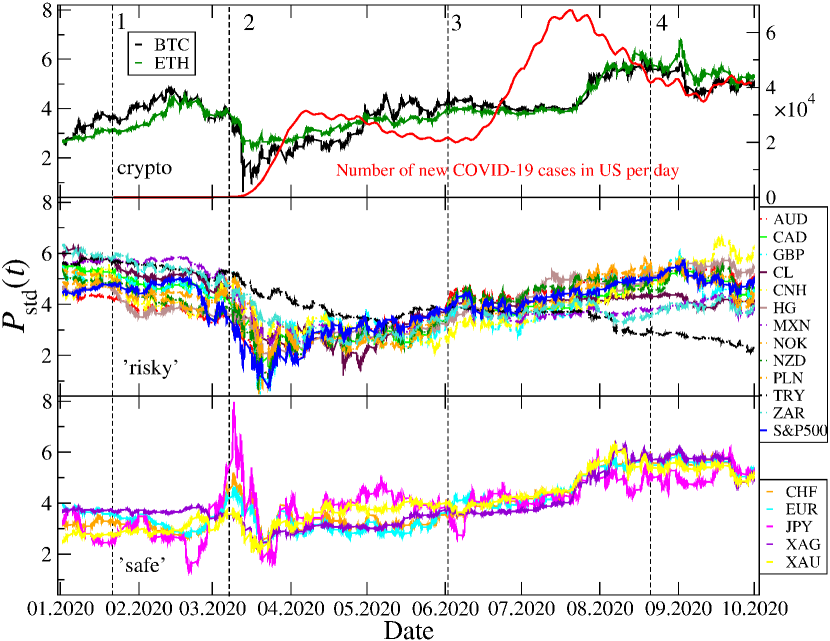
The analysis was carried out for several different time scales but, for the sake of clarity, only two scales are considered here: the shortest available scale min and the scale corresponding roughly to a trading day in the NYSE stock market min (an actual trading day lasts for 390 min). For the return-magnitude filtering parameter also two values are discussed here: , which does not favor any specific magnitude range, and , which amplifies the large return contribution.
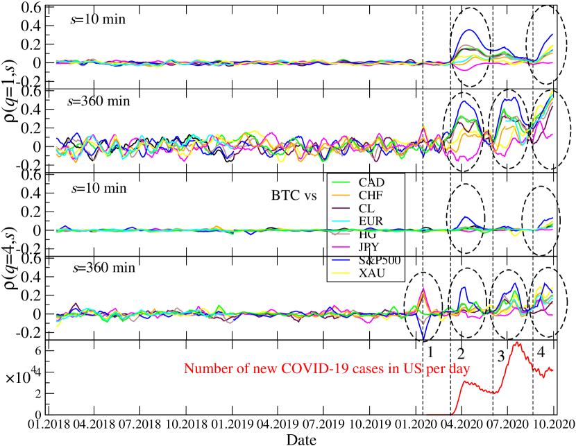
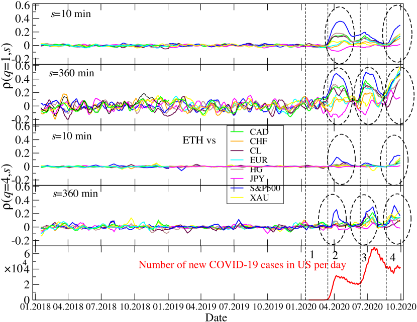
Figs. 58 and 59 display for a combination of the and values described above. In each panel for BTC/USD (Fig. 58) or ETH/USD (Fig. 59) and each of 8 other assets: CAD, CHF, CL, EUR, HG, JPY, S&P500, and XAU are shown. Some of the assets listed in the beginning of this section have been omitted since their cross-correlation with other assets is similar to one of the assets that are shown: NASDAQ100 and DJIA are similar to S&P500, XAG is similar to XAU, the currencies: AUD, NZD, ZAR, CHN, MXN, EUR, GBP, NOK, and PLN are similar to CAD. On the other hand, TRY has been omitted because for almost all the time it was uncorrelated with BTC and ETH.
In accordance with the initial hypothesis, the cryptocurrency market and the traditional assets used to reveal no significant cross-correlation in 2018 and 2019. However, this situation altered in 2020 with 4 specific periods of the statistically significant cross-correlations that can be distinguished. All these periods are related to the Covid-19 pandemic. The first one (see the corresponding number in in Figs. 57–59) was associated with a drop of S&P500 and the other US stock market indices triggered by the first identified local case of Covid-19 on Jan 21, 2020. During this time BTC continued its upward trend, which led to negative for BTC and S&P500 for . At that time, BTC was also positively correlated with some other financial instruments considered safe: JPY, CHF, and gold. Interestingly, the cross-correlation between ETH and the other assets were still insignificant. One could argue that, at that initial Covid-19 phase, BTC fulfilled its planned role as a hedge for risky assets.
This statement is no longer true since the Covid-19-related market panic of March 2020, when almost all financial assets expressed in USD, including the cryptocurrencies, sharply lost their value. The positive cross-correlation between BTC and the traditional assets were the most evident during that time. was larger for min than for min, but nevertheless both were significant. Typical for the cryptocurrency market as it has been reported in Sect. 5.2, such behaviour can be explained by the fact that the cross-correlations need time to build up. In the case of large returns (), BTC was positively cross-correlated with S&P500 mainly, while it was more independent in respect to the other assets. However, generally () BTC is positively cross-correlated also with copper, crude oil, gold, and CAD. There was no substantial cross-correlation between BTC and CHF or EUR, and was negative for BTC vs. JPY. From this point of view, BTC became a risky asset. In March 2020 one could observe similar behaviour of also in the case of ETH, because the global financial market panic did not spare any cryptocurrency.
After transient restoration of the financial markets in April and May, the fear returned in June 2020 with the beginning of the 2nd Covid-19 wave (period 3 in Figs. 57–59). It was accompanied by strong positive cross-correlation of BTC and ETH with the traditional assets except JPY that was observed mostly for min. was smaller for min, but still positive and significant for . What is even more interesting is the behaviour of the detrended cross-correlations in the 4th considered period that started in late Aug 2020 after Covid-19 slowing down in the United States. Since that point BTC and ETH have been positively correlated with all the considered traditional assets, even with JPY, on all considered time scales. BTC, ETH, and the other assets expressed in USD gained value; S&P500 and NASDAQ100 even reached their all-time highs. This surprisingly collective behaviour of the considered financial instruments may be connected with weakness of USD, in which they are expressed. This is visible especially for EUR, which is now one of the most strongly correlated assets with BTC and ETH for min, while it was rather weakly correlated before.
It seems that the events connected with Covid-19 triggered the emergence of cross-correlations between the major cryptocurrencies and the traditional markets. These cross-correlations occurred not only during the sharp market falls earlier in 2020, but also during the still lasting recovery phase. Therefore it may be concluded that the cryptocurrencies have ceased to be an island detached from the traditional markets and become a connected part of the world’s financial markets. This can be a sign of positive verification of the cryptocurrencies during one of the most turbulent periods in the recent years. However, this observation is still fresh, therefore a question of whether it is transient or stable remains open. Especially in the context of a highly inflationary policy adopted by the Federal Reserve and other central banks, which is about substantial increasing of the monetary base (Fig. 2).
6 Correlation matrix and network analysis of cross-correlations
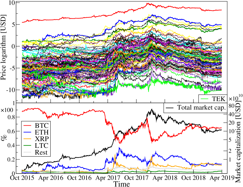
This section discuss a multivariate approach to cross-correlations among the cryptocurrency prices. A data set consists of cryptocurrency daily quotes expressed in USD covering the period 10/2015-03/2019. They form a set of time series of length . A complete list of cryptocurrency tickers and names can be found in the Appendix B. The data source is CoinMarketCap website [25] that collects quotations from all active cryptocurrency trading platforms (273 in March 2019) and evaluates the cryptocurrency prices on an ongoing basis. Prices of the same cryptocurrency from different trading platforms are weighted by their transaction volume with a larger volume corresponding to a larger weight. Fig. 60 shows the individual cryptocurrency price logarithm time series (top panel) and cryptocurrency capitalization (bottom panel), defined as a product of price and the number of issued cryptocurrency units.
By the turn of 2017 and 2018, a systematic increase in the entire market capitalization can be observed. It was followed by a bear market continuing throughout 2018. There were also changes in the individual cryptocurrency market share: by March 2017, BTC capitalization accounted for over of the total cryptocurrency market value, then it fell to around in May 2017, only to rise again to in December 2017. The next two cryptocurrencies in terms of their capitalization, ETH and XRP, moved in the opposite direction. The market share of ETH increased in the first half of 2017, which was related to the ICO-mania discussed earlier. The ICO offers at that time were released on the Ethereum platform mainly and that raised the ETH valuation. In May 2017, the shares of BTC and ETH in the entire market capitalization differed by just a few per cent. The second period of growing ETH importance fell on tip of the ICO-bull market: ETH peaked in January 2018, almost a month after the BTC peak. Fig. 60 presents also a market share of the 4th largest cryptocurrency: LTC. The remaining cryptocurrencies did not account for more than of the entire market capitalization. All the cryptocurrencies considered here account for of the market capitalization.
6.1 Correlation matrix
The analysis starts from a set of time series of logarithmic returns , with Kj denoting cryptocurrencies (), X denoting either a fiat currency (USD) or a cryptocurrency, being sampling interval, and indexing consecutive sampling moments. The log-returns can be normalized
| (28) |
where is standard deviation of . Correlation matrix for a base (crypto)currency X is given by
| (29) |
where is a data matrix of size and denotes matrix transpose. A separate matrix can be constructed for each of available base (crypto)currencies X. Each element of is a Pearson correlation coefficient for a pair of exchange rates K/X–K/X with . As a real symmetric matrix, has real eigenvalues and the same number of the associated eigenvectors :
| (30) |
where the eigenvalues are numbered in the ascending order: … and . Through their components , the eigenvectors can be associated with eigensignals that are linear combinations of the original return time series:
| (31) |
These eigensignals may be associated with respective orthogonal portfolios [195].
A convenient reference for the empirical correlation matrices is the Wishart ensemble of random matrices [196], whose universal properties describe uncorrelated data. Matrices of the Wishart ensemble are constructed as the correlation matrices from time series of i.i.d. random variables with the Gaussian distribution [197]. Analytical form of p.d.f. describing an eigenvalue distribution of is known:
| (32) |
| (33) |
where and , id the length of the time series and is the number of time series. The above relationship is called the Marchenko-Pastur distribution that is strictly valid in the infinite limit [198]. A comparison between the Marchenko-Pastur distribution and the empirical matrix eigenvalue distribution can show how noise and collectivity impacts the cryptocurrency market.
A typical feature of mature financial markets is a dominant share of noise effects in the cross-correlations among financial instruments. In this case an eigenvalue distribution of can be approximated by the Marchenko-Pastur distribution for a majority of the eigenvalues [198]. At the same time, there is usually at least one eigenvalue outside the Marchenko-Pastur distribution [199, 200, 201, 202, 203, 204, 205, 206]. This eigenvalue or these eigenvalues, together with their associated eigenvectors, reflect how collective are the price movements on a given market [8, 96].
6.1.1 Correlation matrix elements
In a generic case of uncorrelated signals, the off-diagonal entries of are Gaussian-distributed with zero mean [196]. However, in the case of empirical correlation matrices, there may be a shift in this distribution (positive or negative mean) and presence of heavy tails [8, 201]. On the cryptocurrency market, the off-diagonal matrix entry distribution largely depends on a base currency as Fig. 61 documents for several representative cases. For all base currencies, this distribution differs from a random case. The smallest deviation is noticeable for X=BTC, which means that the market observed from a BTC perspective is the least correlated. The more peripheral (lower capitalization) a base cryptocurrency is chosen, the more the distribution is shifted to the right with an extreme case of TEK. In this case, all the exchange rate pairs involving TEK as the base give and the distribution mean is located close to 0.9. For such a peripheral cryptocurrency, the market is the most collective. This is even more evident for an artificial cryptocurrency (fict in Fig. 61), whose each exchange rate is driven by a geometric Brownian motion () of . In this situation the distribution is closer to the random matrix case than any other one. The fictitious cryptocurrency volatility is responsible for this behavior: when it increases, the off-diagonal elements are shifted to the right. For the distribution for X=fict looks similar to that obtained for X=TEK.
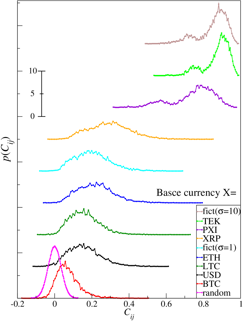
6.1.2 Correlation matrix eigenvalues
PDFs describing the eigenvalue distribution for three base currencies: USD and the two extreme case cryptocurrencies: BTC and TEK are shown in Fig. 62. The following characteristics describing the market cross-correlation structure can be observed: (1) a market factor [205, 206], which shows the average level of cross-correlations (2) a distance between and the rest of eigenvalues, which determines a share of the genuine cross-correlations, and (3) the eigenvalue bulk location in the Wishart region [77]. Value of corresponds to a right-side shift of the average off-diagonal element of in Fig. 61. The smallest shift of occurs for X=BTC. Most of the remaining eigenvalues in this case are located within the limits set by Eq.(33). For X=USD a value of is higher, which means that the cryptocurrency market is more collective if expressed in USD than in BTC. The largest value of is obtained when the cryptocurrencies are expressed in TEK. is responsible for more than of the matrix trace, which effectively “squeezes” the other eigenvalues to around zero. This leads them to “push out” the noise-related eigenvalues even though they still specify random cross-correlations [207].
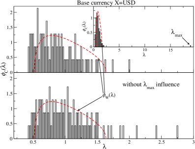
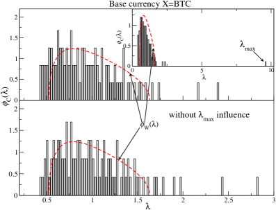
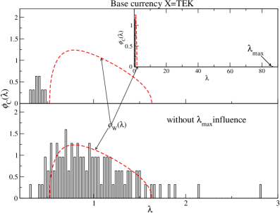
A complementary indicator of collectivity is the eigenvector components corresponding to (Fig. 63). Through a significant contribution of the same sign from all time series (all eigenvector components), they reflect the collective nature of the respective eigenvector. Here, the “squeezing” effect is also visible while preserving the eigenvector corresponding to the second largest eigenvalue . They are shown in Fig. 63 (bottom panels). For X=BTC and X=USD, the eigenvector components have a distribution close to a normal one, while for X=TEK the distribution is dominated by a few components only.
In order to eliminate the “squeezing” effect, the influence of the largest eigenvalue has to be subtracted. This can be accomplished by fitting to each time series the eigensignal with the least-square method:
| (34) |
where and are parameters. A residual correlation matrix that no longer contains a market factor is constructed from the residual time series [206]. The eigenvalue PDFs after eliminating are presented in the lower panels of Fig. 62. In all the cases, the outlying eigenvalue has disappeared and the vast majority of eigenvalues fall within . This observation also applies to the extreme case of X=TEK. The eigenvectors of are different in general from the eigenvectors of (see Fig. 64). For each X their component distribution is approximated well by the normal distribution, exactly as the eigenvector component distribution for the random matrices W.
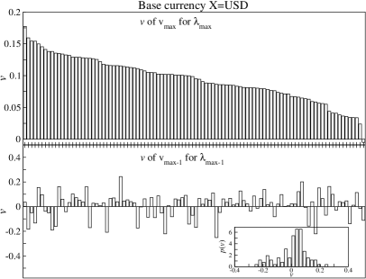
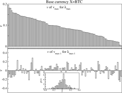
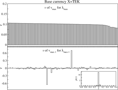
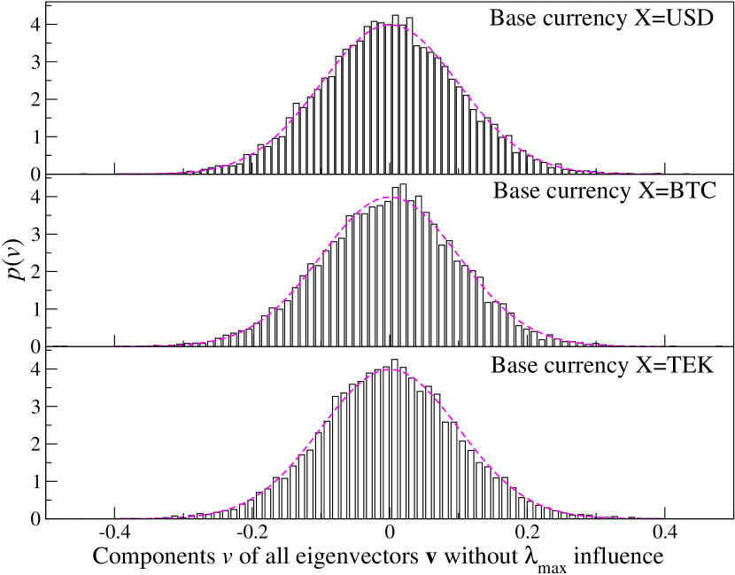
6.1.3 The largest eigenvalue for various base currencies
Fig. 65 displays for all the considered cryptocurrencies treated as the base, together with a fictitious currency created like before (see 6.1.1). This allows one to see what the entire market structure looks like from each cryptocurrency’s perspective. The extremes X=BTC and X=TEK previously shown in detail are the lowermost and the uppermost ladder rungs here. A value of corresponding to a given base currency X should be interpreted as the relative importance of a given cryptocurrency.
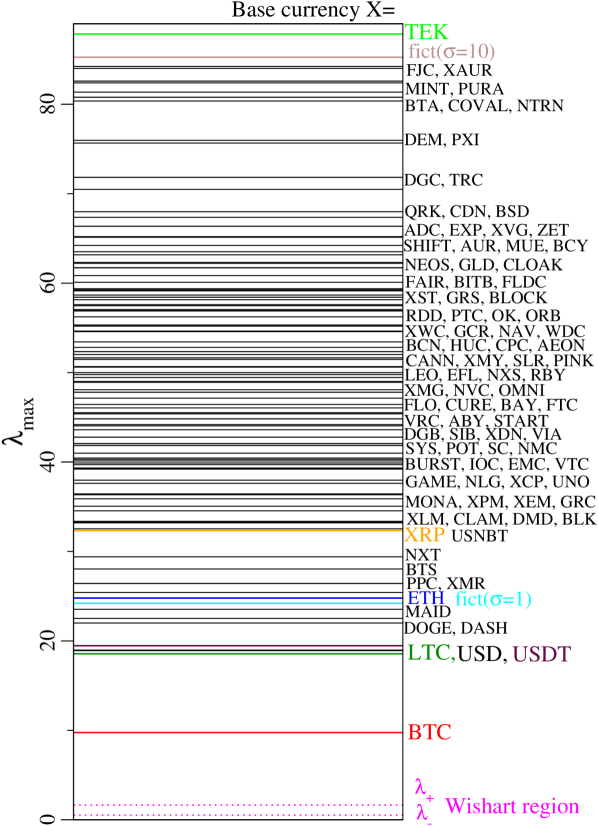
A sharp change in the valuation of a peripheral cryptocurrency that is not correlated with the other cryptocurrencies and has its individual dynamics does not affect their behaviour, but nevertheless it does change values of all the cryptocurrencies expressed in it. As a result, the entire market’s valuation shifts and the cryptocurrencies appear strongly cross-correlated and synchronous. In this case is large. On the other hand, a similar change in the valuation of an important cryptocurrency that have a number of other cryptocurrencies following it results in that the other cryptocurrencies can have their dynamics affected, too. Consequently, any valuation change when the other cryptocurrencies are expressed in this cryptocurrency turns out to be relatively small and the market appears less cross-correlated.
For the fictitious currency (fict()) and USD, is relatively low, because despite having their dynamics independent from the cryptocurrency market, they are characterized by a low volatility level if compared to the cryptocurrencies. Therefore, their small, uncorrelated changes do not affect much the market valuation if they are this valuation base. A situation is completely different when volatility of the fictitious currency is raised to (fict()). Then the largest eigenvalue reaches a high level above 80. A significant change of the fictitious currency value causes shifting of the cryptocurrency valuations expressed in it. Therefore, from an independent, highly volatile currency’s perspective, the market seems substantially collective. The “dragging” effect of a rapid change in a base currency value is shown in section 5.3 and in Ref. [58]. Large volatility of CHF and GBP caused on long time scales a cross-correlation increase among the exchange rates with one of these currencies being the base.
The above interpretation of – the lower its value, the more important the base cryptocurrency X – is also supported by capitalization volume. TEK, for which is the largest, has one of the smallest capitalizations, while BTC has the largest one. In addition, TEK/USD shows a trend that differs from the other cryptocurrencies’ trends (Fig. 60).
6.1.4 Quasi-idempotence
Another measure that can be applied to rank the importance of cryptocurrencies is quasi-idempotence [208]. The underlying notion is to assess how close an experimentally-obtained connectivity, synchronization, or correlation matrix is to the same squared infinitely many times. Considering a weighted network, the corresponding matrix is the least sensitive to squaring (closest to equilibrium) whenever the edge weights are simply reflections of the corresponding node strengths; in other words, when the connectivity between any two nodes is a reflection of their common participation in global connectivity. Quasi-idempotence, therefore, can be deemed an index at the same time of self-similarity and collectivity. Here, it was calculated according to
| (35) |
where and denote the initial correlation matrix for a base (crypto)currency X and the same squared infinitely many times, practically obtained according to a truncation criterion while maintaining unit norm at each step to avoid divergence. yields a vector containing the rearranged off-diagonal elements of with and denotes the element-wise Pearson correlation between the two vectors. As the measure is ill-defined in the presence of negative entries (due to possible non-convergence), anticorrelations were clipped to zero. While related to the largest eigenvalue analysis, this approach is mathematically distinct and entails a more complex dependency on the entire spectrum. Consequentially, as visible in Fig. 66, it not only confirmed but demonstrated even more markedly the centrality of the Bitcoin, such as that the lowest values of were consistently observed when this was taken as the base currency: such a finding underlines that the “collective dynamics” which endow the correlation matrix with a non-random structure largely stem from the influence of this currency. Similar dependencies can be detected in maturing culture neurons, physical networks of chaotic oscillators as well as simulations of stochastic Kuramoto networks [208].
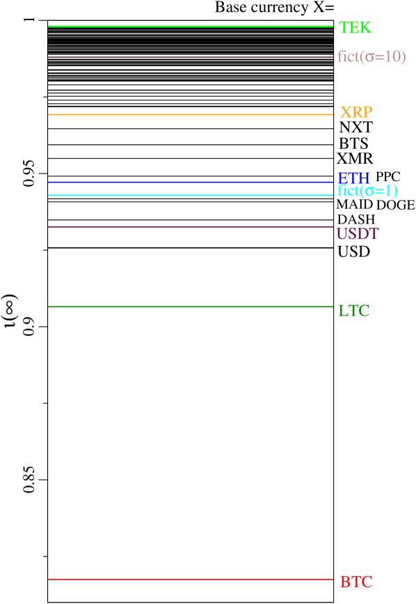
6.1.5 Evolution of the market cross-correlation structure
As characteristics of the individual cryptocurrency exchange rates evolve over time, a cross-correlation structure of the market can also change as the market develops. Top panel in Fig. 67 presents of for X=BTC, X=ETH, X=XRP, X=TEK, X=USD, and X=fict (constructed from a geometric Brownian motion with ) calculated for various base currencies in a half-year (182 days) rolling window with a one-day step. Bottom panel of Fig. 67 presents evolution of a market capitalization share of the most important cryptocurrencies calculated in the same way.
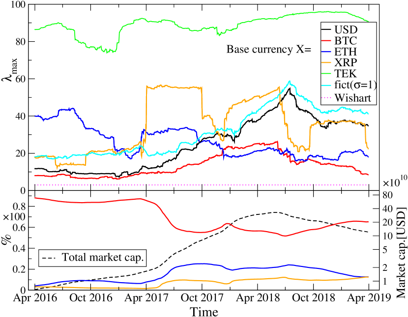
The extreme cases (X=BTC and X=TEK) do not change significantly over time. However, the increase in and, consequently, in the market cross-correlation strength is particularly strong for X=USD and X=fict(), whose dynamics are independent of the cryptocurrency market. The largest growth can be seen in the semi-annual windows ending from January to August 2018 – this interval includes a period of a strong bull market followed by a crash. This behaviour is consistent with an observation that stock markets are strongly collective during sharp declines [8, 209, 210]. After the cryptocurrency market calmed down in the second half of 2018, for USD and fict() decreased, but they still remain above the 2017 level.
If X=ETH one can see a systematic drop in that is due to a capitalization increase of this cryptocurrency (Fig. 67). In the windows ending from December 2017 to June 2018 was lower than , which was a temporary takeover of the dominant role on the cryptocurrency market by ETH. At that time ETH’s share in the market capitalization increased while the BTC’s share dropped, which was related to the ICO-mania mentioned earlier. The number of ICO offers was released mainly on the Ethereum platform which shot up a demand for ETH, rose its importance, and strengthened links with other cryptocurrencies. An additional factor that caused BTC to decline at the turn of 2017 and 2018 was that BTC experienced its valuation peak in December 2017, while the other major cryptocurrencies, including ETH, about a month later. From January 2018 a bear phase spread across the market, with BTC losing relatively less value, which translated into an increase in its market capitalization share. This was accompanied by a systematic decline in , which can be interpreted as a return of the bitcoin’s dominant position.
If X=XRP one can see jumps in (Fig. 67) that were associated with a 102% increase in the XRP/USD rate valuation on 04/02/2017. Such a big change implied valuation change of all the cryptocurrencies expressed in XRP, leading to a collective behaviour of the entire market if observed from the XRP perspective. Inclusion of that day in a semi-annual rolling window translates directly into a sharp increase in . In contrast, a decline in half a year later was caused by falling out of that day from the rolling window. This confirms the previously presented interpretation of the largest eigenvalue magnitude.
6.2 Minimal spanning tree representation of the cryptocurrency market
Based on the correlation matrix , one can also construct a network representation of the market. Nodes can represent the exchange rates and edges can be the cross-correlations between two exchange rates with weights equal to .
Minimal spanning tree (MST) is a connected subset of a weighted network that spans this network and minimizes a sum of the metric edge lengths. It was first applied to a cross-correlation analysis of a stock market in Ref. [7] and, since then, it has been successfully used to analyze cross-correlation topology of various markets such as: Forex [211, 212, 213, 193, 214, 215], the stock market [216, 217, 218, 219, 220, 221, 222, 223, 165], the commodity market [11], and the cryptocurrency market [73]. For the mature markets, a node degree PDF for MST can be approximated by a power-law tails [96]. In the case of the stock and Forex markets, the tail scaling exponents assume values that are similar to the hierarchical models of complex networks [224].
Because the off-diagonal elements of do not meet the metric conditions, it is necessary to transform edge weights into internode distances defined by
| (36) |
that already fulfill these conditions [7]. Since the Pearson correlation coefficient takes values in , the distance is confined to . With this measure, the MST graphs that represent market structure can be constructed by following the Prim’s algorithm [225].
Fig. 68 presents a strongly centralized MST for X=USD, constructed from a set of X/USD exchange rates recorded daily over the period 10/2015–03/2019. is multiplicity (degree) of a node corresponding to BTC/USD, while other nodes have multiplicity not exceeding 10. The node degree can be interpreted as a centrality measure expressing a relative importance of the exchange rate. The larger degree of a node corresponding to a given cryptocurrency, the more it affects the remaining cryptocurrencies [214]. Dominance of BTC in the structure of MST for USD as the base currency is consistent with the already-discussed results of the largest eigenvalue analysis (Fig. 6.1.3).
MST for X=USD, whose dynamics is not directly related to the cryptocurrency market, seems to best describe the market topology. However, as shown in Sect. 6.1, the cross-correlation structure depends heavily on the base currency choice. Fig. 69 shows MST for X=BTC, which looks profoundly different. It is much more decentralized and there is no dominant node. The largest degree is observed for BTS/BTC and MAID/BTC. For the entire period under consideration, MSTs created for the base cryptocurrencies less important than BTC are even more centralized than that for X=USD: most nodes have a unit degree and they are connected to BTC. Results for all the cryptocurrencies used as the base ones are presented in Sect. 6.3.
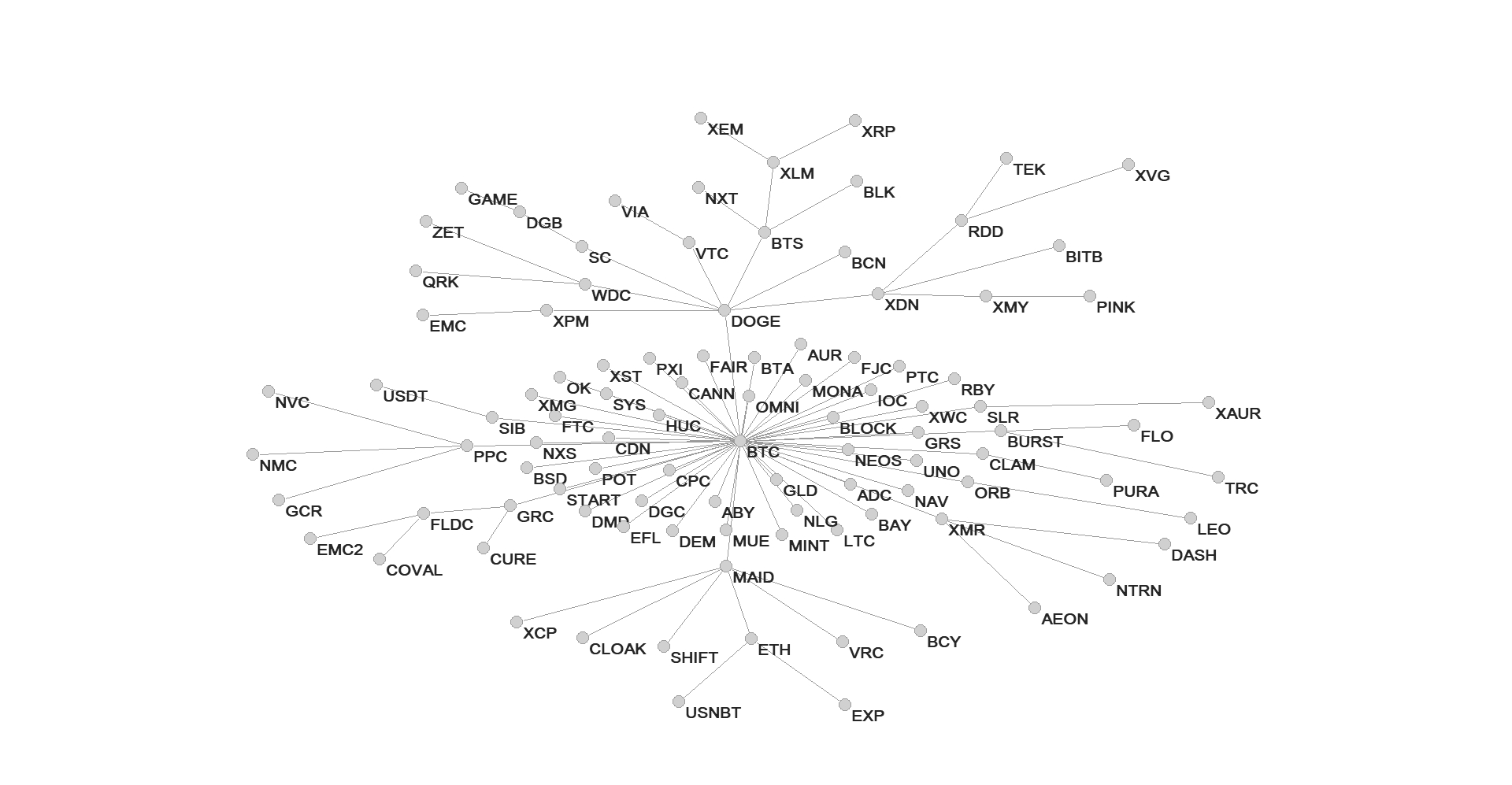
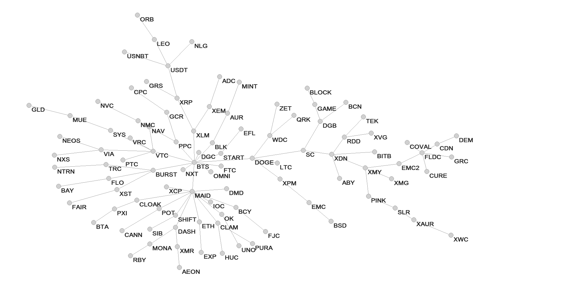
On Forex, the node degree distributions are in agreement with the power-law model, which means that these trees are scale-free for some base currencies [193, 214]. Scaling of the node degree CDF can be parameterized by an exponent :
| (37) |
where is the MST node degree and X base cryptocurrency. Fig. 70 presents a node degree CDF for three base cryptocurrencies with the largest capitalization: X=BTC, X=ETH, and X=XRP together with X=USD. Due to the changing market cross-correlation structure observed in Sect. 6.1.5, the results were also shown in semi-annual windows, apart from the entire-period case from 10/2015 to 03/2019.
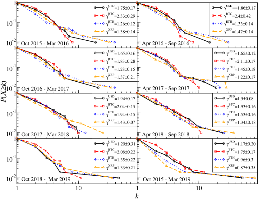
For the whole considered period (bottom right panel in Fig. 70) some trace of scaling can be identified only for X=BTC. In other cases a node with the largest degree, that is BTC, disrupts scaling, because the corresponding MSTs are highly centralized. In a majority of the semi-annual intervals, there is no satisfactory scaling quality, either. Only for X=BTC in some intervals, oscillates around 2, which is a value associated with a decentralized network topology. A significant scaling quality improvement occurs in the interval 10/2017 to 3/2018. A related event is the BTC significance decline described in Sect. 6.1.5 with the associated maximum node degree decreasing for BTC. This made it possible to develop a hierarchical structure of the nodes with the scaling tails of the node degree CDFs. An example of such a situation is X=XRP with and a well-developed scale-free tail. Slightly worse scaling is seen for a subsequent window 04/2018–09/2018, where . In that interval a CDF scaling is also noticeable for X=USD. The last semi-annual window 10/2018–03/2019 displays a return of the BTC domination and, thus, a transition of the MST structure to a centralized form.
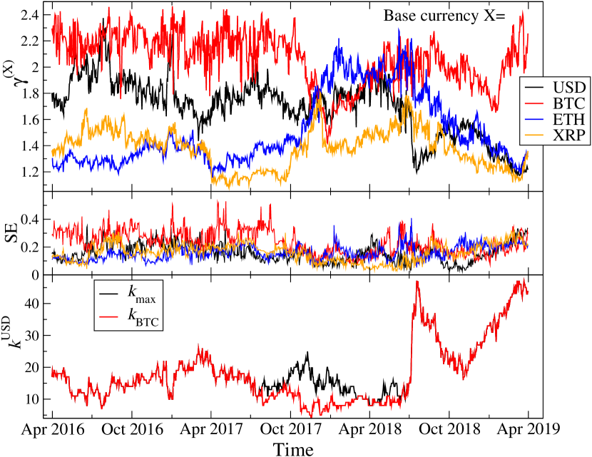
Evolution of the scaling exponent for the above-mentioned base currencies X is presented in Fig. 71 (top panel). A semi-annual rolling window with a step of 1 day is applied. A scaling quality improvement measured by a power-law fit standard error can be observed in the rolling windows that end between 10/2017 and 5/2018 (middle panel) and it corresponds to the period of the interim BTC/USD market capitalization share and node degree decline (bottom panels of Fig. 71 and Fig. 71). On contrary, in the windows that end between 8/2017 and 4/2018, there are nodes with a larger degree than BTC/USD. This is related to a strong bull market that started on all cryptocurrencies. During that time, the market was increasingly collective from the X=USD perspective as shown in Fig. 67. Between 11/2017 and 3/2018, increased above 2, which corresponded to a dominant role takeover by ETH (see also Fig. 67 for behaviour). This change was associated with the ICO-mania and the increasing capitalization and the ETH significance. Between 5/2018 and 7/2018, which was the final phase of the bull market, the market became decentralized and , , and were above 1.8. However, was equal to around 1.6 at that time, which is close to the theoretically derived value for a hierarchical network model: [226, 227].
The CDF tails lose their scale-free form when BTC dominance returns. This can be seen in the windows that end in 07/2018 in a form of a sharp jump in , which is the BTC/USD node (bottom panel of Fig. 71). The BTC/USD node degree increased by a factor of 5 when 1/7/2018 fell out of the corresponding semi-annual window. On that day BTC’s valuation dropped down by 5%, while ETH’s valuation increased by 10%. Other large-capitalization cryptocurrencies also rallied on that day. The market MST returned to its centralized topology.
6.3 The largest eigenvalue vs. MST maximum node degree
Interpretations of and are mutually related. Expressing cryptocurrency values in a base currency X of large capitalization takes some cross-correlation contribution that is associated with the dynamics of X. From the perspective of a dominant cryptocurrency, the market seems to be rather weakly collective and the corresponding network representation is decentralized. On the other hand, if one expresses other cryptocurrencies in a base currency with its own dynamics, the market is collective and the network is strongly centralized.
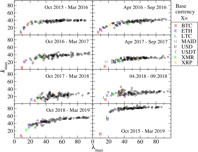
Fig. 72 shows vs. for all the possible choices of the base currency X calculated in fixed semi-annual windows and over the whole interval 10/2015–3/2019 (bottom left). Each circle or letter denotes different X. (Instead of that describes the CDF tail scaling property, the maximum node degree is used here. This replacement is necessary because for the most choices of X, the scaling quality was not sufficient. It does not alter the interpretation, however.) If a base cryptocurrency is located in the bottom left corner of a plot, its hierarchical position in the market structure is dominant. In all the periods, except for 10/2017–3/2018, BTC holds a dominant position. During 10/2017–2/2018 one could also observe the lowest value of , located below the level of . This allowed for the formation of a hierarchical structure with the power-law node degree CDF, which disappeared after the bull market ended in 1/2018 and BTC’s dominance returned (Fig. 72).
While considering the whole interval, one can observe the highest for a vast majority of the base cryptocurrencies (bottom right panel of Fig. 72). This is consistent with the fact that the most nodes are connected to the BTC/USD node and have unit degree, which gives the overall centralized structure of MST. BTC seems to dominate the cryptocurrency market in a way much more significant than USD does [22, 193, 214], which makes it the most natural base for this market.
6.4 Cryptocurrency network topology on Binance
In order to extend sensitivity of the network approach, the MST formalism is a method at hand [165]. It allows one to unveil the network properties on various time scales and from a perspective of different fluctuation amplitudes (selected by means of a parameter). A construction scheme for MST is parallel to the original MST except for a distance that has to be calculated from the detrended cross-correlation coefficient defined by Eq.(15) in Sect. 4.1.2. It inherits ’s dependence on the parameters and :
| (38) |
Only positive values of are considered ( and ), which guarantees that is a metric [165].
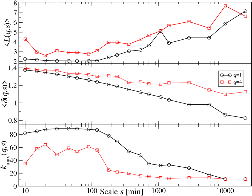
MST are formed from cryptocurrency exchange rate quotes from the Binance platform (a detailed list is given in the Appendix C). Time series of returns were sampled with 1 min resolution and cover the whole year 2018. Trading on Binance occurs predominantly on the exchange rates where BTC is the base. In 2018 there were 93 such exchange rates. The second most frequently traded cryptocurrency was ETH (90 exchange rates). It was also possible to obtain 30 exchange rates expressed in Binance coin (BNB) and 8 exchange rates expressed in USDT, but here there are only considered those involving BTC. This choice preserves dynamics of the individual cryptocurrencies without being distorted by evolution of the strongest one (see Sect. 6.1.3). Because of fixing X=BTC, the BTC superscript is dropped in all quantity symbols for clarity.
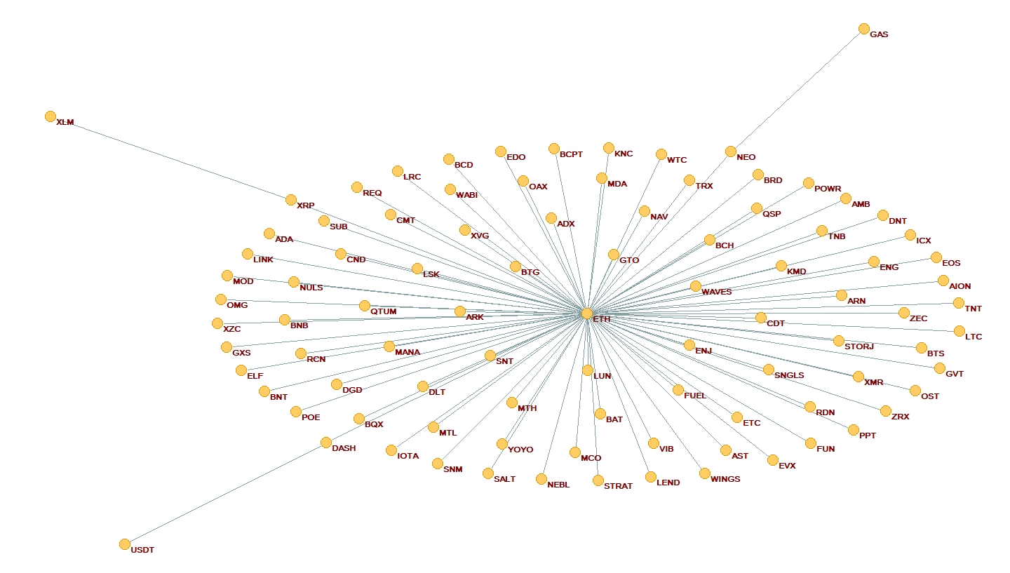
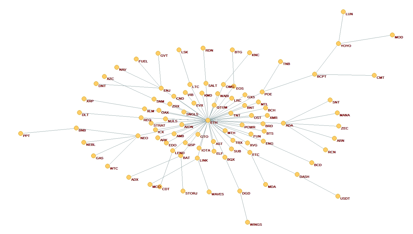
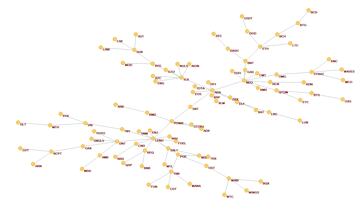
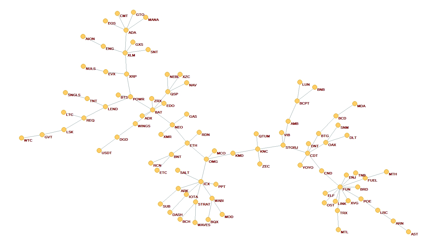
Mean distance decreases with increasing (middle panel in Fig. 73), which is a natural consequence of the increased cross-correlation strength on longer time scales (Sect. 5.2). In contrast, it increases with . The average shortest path length calculated for binary edges (i.e., the MST edges are considered as unweighted here) increases with and it is larger for than for , which indicates that MST becomes less centralized for large returns (top panel in Fig. 73). The MST topology shows a kind of “phase transition” for min. Below this scale it is almost perfectly centralized for with and and significantly centralized for with and . The central node represents always ETH or, more precisely, the exchange rate ETH/BTC (Fig. 74), because for short time scales the information flow enters the market principally through the most actively traded cryptocurrency – ETH. The situation looks different for the time scales longer than 120 min, because for such scales the ETH hub loses centrality and MST becomes decentralized gradually (Fig. 73). For the longest considered time scale of 2 weeks drops below 20 for both and . The corresponding MSTs are distributed (Fig. 75).
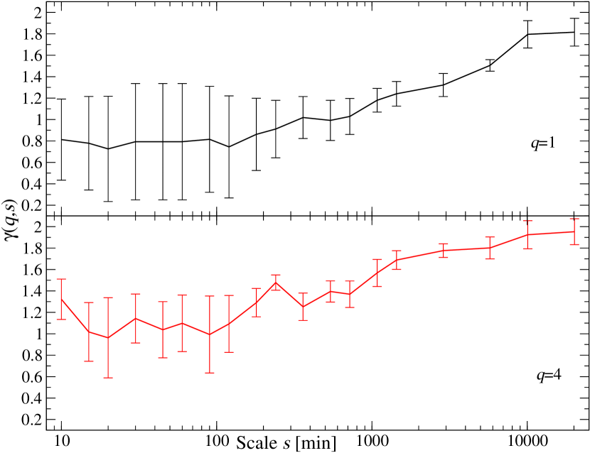
Despite the fact that for the shortest scales min, the results are statistically significant. This was checked by calculating and their standard deviation for 100 realizations of surrogate data (randomly shuffled returns of 93 exchange rates). Only in a few cases exceeded threshold.
The above observations are supported by the scaling properties of the MST node degree CDFs. For each and , the corresponding CDF tails were approximated by a power-law function with the exponent (Eq.(37)). Fig. 76 shows values of this exponent together with the standard error of a linear regression fit. Up to min, one does not observe any power-law scaling (large error bars) with a dominant role of the ETH node being responsible for this behaviour (see Fig. 75). However, for min the maximum node degree decreases and the node degree CDF reveal a scaling tail (a smaller error, Fig. 76). The exponent increases with increasing reaching values higher than 1.8 for week, which are characteristic for decentralized networks.
The MSTs reach topology of the hierarchical network model [226, 227] corresponding to later for ( min) than for ( min). This is because for large returns the cryptocurrency exchange rates are globally less correlated than for medium returns, which opens more space for the formation of sub-clusters in MSTs for . This result shows that a standard MST construction () offers too little sensitivity and it is thus inferior to the MST approach.
The network approach presented here for X=BTC confirms the results reviewed in earlier sections according to which the cross-correlation between the cryptocurrency exchange rates tend to increase with increasing time scales because of the fact that less frequently traded exchange rate pairs need time to synchronize. With increasing scale, the MST structure becomes more diverse and decentralized. A dominant position of ETH observed for short scales disappears and a hierarchical structure develops. This happens faster for large returns than for medium ones because the cross-correlations are weaker for the former.
7 Summary and conclusions
A striking development of the cryptocurrency market in the last several years – from a small and peripheral market to a market at the level of a middle-size stock exchange capitalization – provides a unique opportunity to observe its quick structural self-organization. Availability of the high frequency data allows one to conduct advanced statistical studies of the processes governing the market evolution from its birth to the present.
In this review we presented the most important results derived from a few studies carried out based on available high-frequency data from the cryptocurrency exchange platforms. A main stress was put on methods known well from statistical physics like the detrended fluctuation analysis with its multifractal extensions quantifying nonlinear dependencies in data and the cross-correlation matrix analysis exploiting universal predictions of the random matrix theory and the complex network theory.
A principal conclusion that can be inferred from the presented results is that the cryptocurrency market has gradually been pursuing its way to maturity. It is still not a fully developed market unlike, for example, Forex, since there are still significant differences between both as regards liquidity and the number of transactions, among others. The following characteristics of the market were also discussed in detail: the leptokurtic tails of the return probability distribution functions, the long memory in volatility, the antipersistent dynamics of the returns, the multiscale auto- and cross-correlations between the cryptocurrency exchange rate returns in respect to other cryptocurrencies and the fiat currencies like USD and EUR. Behaviour of the exchange rates on different trading platforms was also a subject of interest.
All these properties, known together as the financial stylized facts, characterize mature financial markets with the stock markets, the commodity markets, and the foreign currency market, among others. In contrast, on developing/emerging markets some or all these properties may not be observed at all. Thus, their existence (or lack thereof) can determine a development stage of a particular market. On the cryptocurrency market one observes a gradual shift from an early, immature stage prior to 2014 towards more developed stages after that year with some parts of the market reaching even a stage of the almost-complete maturity. These parts consist predominantly of the exchange rates involving bitcoin (BTC), ethereum (ETH), a and several other the most liquid cryptocurrencies like ripple (XRP) and litecoin (LTC). That shift was caused by a significant increase of the trading volume and frequency that was seen on the market over the years. This observation points out to these quantities as the principal driving factors of market development.
More specifically, as regards the most mature and long-traded part of the market, i.e., the exchange rates BTC/USD and ETH/USD, the return autocorrelation function was changing its form from short-term memory to long-term one with a power-law decay. In parallel, the return CDF tails lost their initial Lévy-stable form with the exponent form and became inverse cubic power law ( or even less). As mentioned above, these shifts took place around 2013-2014 and after that both characteristics do not differ from mature markets. An analogous change of dynamics happened in 2017, when the Hurst exponent rose from to , i.e., from the antipersistent regime typical for developing markets to the neutral regime proper to mature markets. The same was visible for the multiscale autocorrelations – the singularity spectra change shape from a strong left-side asymmetry seen till 2017 to a mature, symmetric form in 2018. As in other markets, multiscaling is observed for large returns, but, contrary to that, the smaller returns are monofractal here unlike the corresponding returns on Forex and other mature markets.
One of the key features of Forex is possibility of expressing any currency in any other currency. On cryptocurrency market such a possibility emerged gradually as new trading platforms became available. Initially, only the exchange rates involving main fiat currencies were traded, but after a few years the cryptocurrencies could also be expressed in each other without participation of the traditional currencies. In this case the most liquid exchange rate – BTC/ETH – reveal autocorrelation that resembles the autocorrelation of EUR/USD. However, like in immature markets, was still left-side asymmetric even in the second half of 2018. Multiscaling and other stylized facts might be viewed as indicators of market complexity. Therefore, a process of market maturing is inevitably associated with complexity increase. A feature that can also be considered in this context is multiscale cross-correlations among the exchange rates. Such cross-correlations were found at the level of medium and large returns and their strength increases with increasing scale (unlike Forex, where such dependence is much weaker). Moreover, for a fixed scale, the detrended cross-correlations were getting stronger over the years, which is especially evident for small scales. This is associated with reduction in the triangular arbitrage opportunities. The less opportunities are detectable, the more liquid and mature the market is, because lack of liquidity slows a rate of information spreading. Since the cryptocurrency market is decentralized and since liquidity varies among the trading platforms, different platforms display different stage of the market maturity – a feature unique for this market.
The strength of the multiscale detrended cross-correlations among the exchange rates depends crucially on whether the two exchange rates involve a common base (crypto)currency – if this is the case, they are substantially stronger. There is a hierarchical structure of cross-correlations in the market: one can identify the exchange rate clusters consisting of stronger-than-average correlated rates – typically those that remain in a triangle relation with each other. Because of a slower information flow, the clusters do not comprise the exchange rates without triangle relationship, which is a feature distinct from Forex, where there are other factors that correlated currencies, like the geographic proximity.
At present it is still too early to discuss whether the cryptocurrency market will survive for a substantial period of time or in which direction it may evolve except for that it is very likely that its liquidity can improve constantly in the following years. One of the key reasons is that despite its high volatility level at present, this market offers new investment opportunities, thus actually facilitating portfolio diversification. Here an important role is played by the most liquid cryptocurrencies, ETH and BTC, which, if chosen for the exchange rate base, decollectify the market and, in turn, allow one for further portfolio diversification within the cryptocurrency market itself. These cryptocurrencies seem to be also the most mature ones and thus the most credible.
In this context the results that is among the most important is a kind of “phase transition” that has been noticed recently in 2020 during the Covid-19 pandemic. The cryptocurrency market evolution used to show no cross-correlation with the evolution of the traditional markets: the prices of BTC or ETH and other financial instruments like the fiat currencies, stock indices, and commodities were uncorrelated on average. However, this suddenly changed during this year’s turmoil observed on the markets that was related to the Covid-19 outburst: the major cryptocurrency prices became cross-correlated. First, the positive cross-correlations were seen with the instruments considered safe, like Japanese yen, but later such cross-correlations appeared also with rather the risky instruments like S&P500, typical currencies, and commodities. Interestingly, this occurred not only during the market panic at the 1st pandemic wave in early Spring 2020, but also during the recovery phase experienced by the traditional markets in late Spring and even during the pandemic slowdown in Summer 2020. It seems that the cryptocurrency market ceased to be viewed as a “safe haven” by the investors and become a part of the network constituting the global market. It is an important question whether this coupling is a transient feature only or, maybe, it is another manifestation of the market’s maturation and it will continue to be observed in future.
Appendix A Full names and statistical properties of cryptocurrencies from Binance and Kraken
| Ticker | Full name |
|---|---|
| BAT | Basic Attention Token |
| BCH | Bitcoin Cash |
| BTC | Bitcoin |
| BNB | Binance coin |
| DASH | Dash |
| ETC | Ethereum Classic |
| ETH | Ethereum |
| ICX | ICON |
| LSK | Lisk |
| LTC | Litecoin |
| MIOTA | IOTA |
| NEO | NEO |
| REP | Augur |
| USDT | Tether |
| XLM | Stellar |
| XMR | Monero |
| XRP | Ripple |
| ZEC | Zcash |
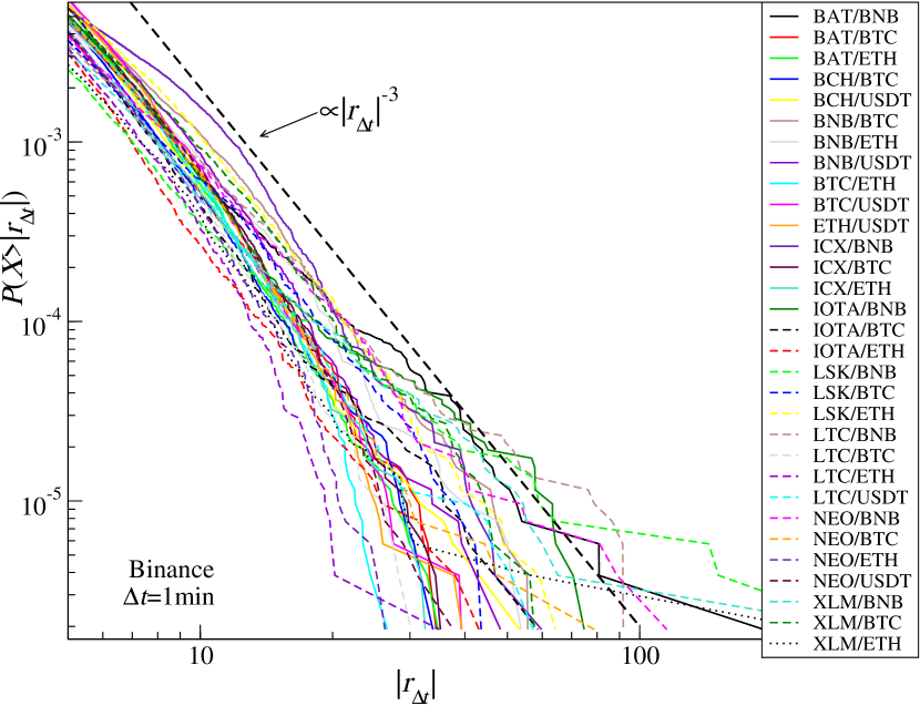
| Name | |||||
|---|---|---|---|---|---|
| BTC/USDT | 3,450,1 | 1,07 | 8559 | 196331 | 0,47 |
| ETH/USDT | 3,390,1 | 1,10 | 16184 | 61430 | 0,48 |
| BTC/ETH | 3,300,1 | 1,09 | 12134 | 60824 | 0,51 |
| BNB/BTC | 2,670,2 | 1,26 | 40098 | 18634 | 0,43 |
| BCH/BTC | 3,360,1 | 1,25 | 29973 | 16299 | 0,48 |
| BNB/USDT | 3,080,15 | 1,20 | 31320 | 16268 | 0,46 |
| BCH/USDT | 3,360,1 | 1,40 | 40922 | 15893 | 0,48 |
| ICX/BTC | 3,150,1 | 1,58 | 77707 | 15336 | 0,45 |
| NEO/USDT | 3,290,1 | 1,27 | 42709 | 14830 | 0,47 |
| XLM/BTC | 2,710,15 | 1,33 | 67637 | 14556 | 0,46 |
| NEO/BTC | 3,170,15 | 1,34 | 61330 | 14445 | 0,46 |
| LTC/BTC | 3,420,1 | 1,17 | 34360 | 13110 | 0,47 |
| LTC/USDT | 3,230,15 | 1,29 | 45208 | 11793 | 0,47 |
| IOTA/BTC | 3,260,15 | 1,30 | 52793 | 7928 | 0,45 |
| NEO/ETH | 3,540,1 | 1,94 | 80537 | 3765 | 0,42 |
| ICX/ETH | 3,240,15 | 2,20 | 87489 | 3496 | 0,42 |
| BNB/ETH | 2,740,2 | 1,47 | 65950 | 2755 | 0,45 |
| XLM/ETH | 2,960,2 | 1,95 | 85581 | 2580 | 0,43 |
| LSK/BTC | 2,720,15 | 1,94 | 92975 | 2489 | 0,44 |
| BAT/BTC | 3,120,15 | 1,85 | 88702 | 2166 | 0,45 |
| LTC/ETH | 3,610,15 | 2,18 | 93044 | 1825 | 0,42 |
| LSK/BNB | 2,390,35 | 10,27 | 44317 | 1595 | 0,41 |
| IOTA/ETH | 3,520,15 | 2,29 | 91798 | 1495 | 0,43 |
| NEO/BNB | 2,540,2 | 3,66 | 87796 | 1294 | 0,40 |
| LTC/BNB | 2,320,25 | 3,86 | 88053 | 830 | 0,41 |
| BAT/ETH | 3,480,15 | 2,93 | 95765 | 516 | 0,41 |
| LSK/ETH | 2,750,15 | 4,19 | 81720 | 451 | 0,39 |
| ICX/BNB | 2,510,2 | 4,80 | 76597 | 260 | 0,36 |
| IOTA/BNB | 2,880,25 | 4,35 | 81816 | 130 | 0,39 |
| BAT/BNB | 2,700,3 | 6,84 | 61754 | 72 | 0,36 |
| XLM/BNB | 2,590,3 | 3,65 | 90019 | 12 | 0,37 |
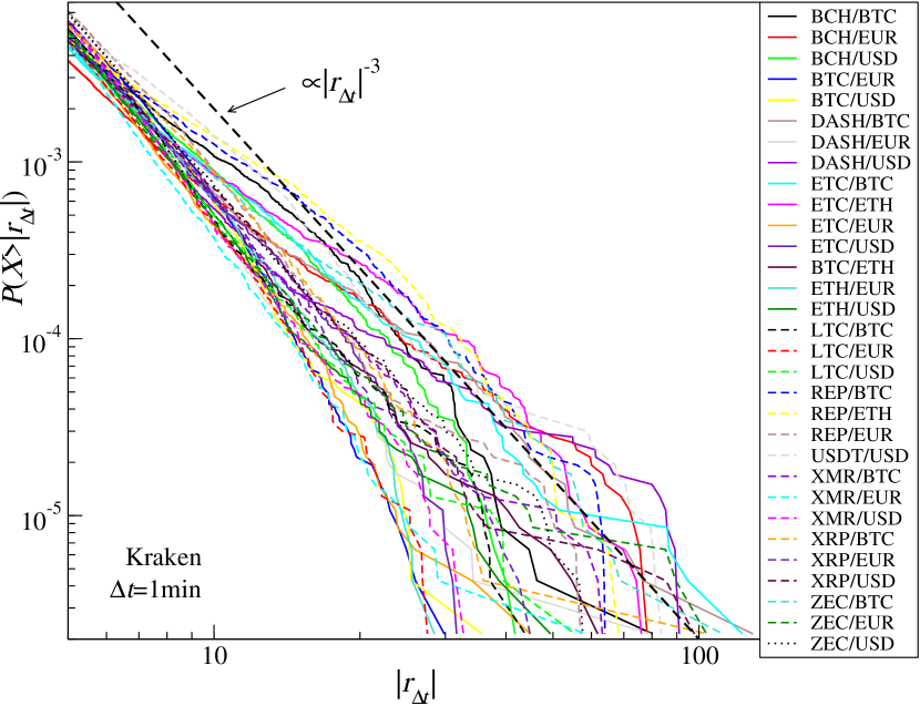
| Name | |||||
|---|---|---|---|---|---|
| BTC/EUR | 3,610,1 | 1,49 | 44310 | 35599 | 0,48 |
| BTC/USD | 3,630,15 | 1,61 | 55360 | 33998 | 0,48 |
| ETH/USD | 3,40,1 | 1,78 | 67807 | 19711 | 0,49 |
| ETH/EUR | 3,370,15 | 1,65 | 61097 | 18171 | 0,49 |
| XRP/EUR | 3,140,15 | 2,28 | 77480 | 7321 | 0,46 |
| XRP/USD | 2,860,2 | 2,69 | 80418 | 6259 | 0,46 |
| BTC/ETH | 3,180,2 | 2,62 | 82074 | 5250 | 0,48 |
| XRP/BTC | 2,990,15 | 3,50 | 72556 | 2763 | 0,45 |
| BCH/USD | 2,610,15 | 3,83 | 75427 | 2151 | 0,48 |
| BCH/EUR | 2,280,3 | 3,31 | 82295 | 2036 | 0,47 |
| USDT/USD | 2,370,3 | 8,97 | 43821 | 1747 | 0,31 |
| LTC/EUR | 3,610,1 | 3,11 | 84104 | 1732 | 0,48 |
| LTC/USD | 3,410,1 | 3,48 | 79983 | 1722 | 0,47 |
| BCH/BTC | 2,350,15 | 4,39 | 68059 | 1251 | 0,43 |
| ETC/USD | 3,160,15 | 4,18 | 74681 | 1114 | 0,47 |
| ETC/EUR | 3,530,15 | 4,01 | 75596 | 973 | 0,47 |
| LTC/BTC | 3,340,15 | 5,09 | 62675 | 940 | 0,45 |
| XMR/EUR | 3,770,15 | 4,16 | 76277 | 865 | 0,49 |
| XMR/USD | 3,730,2 | 5,58 | 63385 | 864 | 0,49 |
| ETC/BTC | 2,310,2 | 6,34 | 55647 | 709 | 0,45 |
| XMR/BTC | 3,210,15 | 6,58 | 54832 | 614 | 0,43 |
| DASH/EUR | 3,590,15 | 6,47 | 57268 | 526 | 0,48 |
| DASH/BTC | 2,520,2 | 7,58 | 49134 | 416 | 0,44 |
| ZEC/USD | 3,180,2 | 7,45 | 51105 | 354 | 0,48 |
| DASH/USD | 2,810,3 | 9,36 | 42727 | 394 | 0,47 |
| REP/EUR | 3,090,25 | 6,79 | 54740 | 374 | 0,45 |
| ZEC/EUR | 3,250,25 | 6,20 | 59369 | 345 | 0,47 |
| ZEC/BTC | 2,290,25 | 7,51 | 51170 | 345 | 0,42 |
| ETC/ETH | 2,180,2 | 9,15 | 41861 | 266 | 0,41 |
| REP/BTC | 2,050,25 | 8,43 | 46419 | 247 | 0,41 |
| REP/ETH | 2,000,3 | 11,57 | 35701 | 158 | 0,40 |
| Triangle | Mean | Max |
|---|---|---|
| BTC-USDT-BNB | 0,00096 | 0,0465 |
| BTC-USDT-ETH | 0,00059 | 0,0367 |
| BTC-USDT-LTC | 0,00087 | 0,0931 |
| BTC-USDT-NEO | 0,00097 | 0,1029 |
| BTC-USDT-BCH | 0,00129 | 0,0793 |
| BNB-ETH-USDT | 0,00126 | 0,0582 |
| LTC-ETH-USDT | 0,00127 | 0,0955 |
| NEO-ETH-USDT | 0,00131 | 0,0435 |
| LTC-BNB-USDT | 0,00203 | 0,2517 |
| NEO-BNB-USDT | 0,00222 | 0,2924 |
| ETH-BAT-BTC | 0,00255 | 0,1249 |
| ETH-BNB-BTC | 0,00108 | 0,0631 |
| ETH-BNT-BTC | 0,00286 | 0,0889 |
| ETH-ETC-BTC | 0,00139 | 0,0630 |
| ETH-ICX-BTC | 0,00148 | 0,0823 |
| ETH-IOTA-BTC | 0,00159 | 0,0699 |
| ETH-LSK-BTC | 0,00243 | 0,2139 |
| ETH-LTC-BTC | 0,00115 | 0,05458 |
| ETH-NEO-BTC | 0,00115 | 0,09129 |
| ETH-XLM-BTC | 0,00138 | 0,71637 |
| BTC-BAT-BNB | 0,00447 | 0,57722 |
| BTC-ICX-BNB | 0,00343 | 0,2256 |
| BTC-IOTA-BNB | 0,00266 | 0,23356 |
| BTC-LSK-BNB | 0,00486 | 1,16489 |
| BTC-LTC-BNB | 0,00185 | 0,24864 |
| BTC-NEO-BNB | 0,00204 | 0,284 |
| BTC-XLM-BNB | 0,00228 | 0,7974 |
| ETH-BAT-BNB | 0,00483 | 0,5747 |
| ETH-ICX-BNB | 0,00355 | 0,2288 |
| ETH-IOTA-BNB | 0,00292 | 0,24176 |
| ETH-LSK-BNB | 0,00519 | 1,16722 |
| ETH-NEO-BNB | 0,00227 | 0,28951 |
| ETH-XLM-BNB | 0,00258 | 0,79693 |
| Triangle | Mean | Max |
|---|---|---|
| BTC-EUR-ETH | 0,00112 | 0,0776 |
| BTC-EUR-BCH | 0,00186 | 0,2003 |
| BTC-EUR-DASH | 0,00131 | 0,2087 |
| ETC-EUR-ETH | 0,00160 | 0,1586 |
| ETC-EUR-BTC | 0,00149 | 0,2449 |
| BTC-EUR-XMR | 0,00146 | 0,1258 |
| BTC-EUR-LTC | 0,00129 | 0,1359 |
| BTC-EUR-XRP | 0,00156 | 0,1919 |
| BTC-EUR-REP | 0,00176 | 0,2080 |
| ETH-EUR-REP | 0,00184 | 0,2920 |
| BTC-EUR-ZEC | 0,00139 | 0,2408 |
| BTC-USD-ETH | 0,00121 | 0,1147 |
| BTC-USD-BCH | 0,00179 | 0,1852 |
| BTC-USD-DASH | 0,00126 | 0,2179 |
| ETC-USD-ETH | 0,00159 | 0,1671 |
| ETC-USD-BTC | 0,00145 | 0,2415 |
| BTC-USD-XMR | 0,00138 | 0,1187 |
| BTC-USD-LTC | 0,00124 | 0,1336 |
| BTC-USD-XRP | 0,00155 | 0,2269 |
| BTC-USD-ZEC | 0,00133 | 0,2203 |
| ETC-ETH-BTC | 0,00119 | 0,2459 |
| REP-ETH-BTC | 0,00139 | 0,3511 |
Appendix B List of 100 cryptocurrency names from CoinMarketCap
| Ticker | Full name | Ticker | Full name |
|---|---|---|---|
| BTC | Bitcoin | GAME | GameCredits |
| ETH | Ethereum | GCR | Global Currency Reserve |
| XRP | Ripple | GRC | GridCoin |
| LTC | Litecoin | NLG | Gulden |
| XLM | Stellar | LEO | LEOcoin |
| USDT | Tether | MINT | MintCoin |
| DASH | Dash | NMC | Namecoin |
| XMR | Monero | MUE | MonetaryUnit |
| XEM | NEM | XMY | Myriad |
| BCN | Bytecoin | NAV | NavCoin |
| BTS | BitShares | NTRN | Neutron |
| DGB | DigiByte | OK | OKCash |
| XVG | Verge | OMNI | Omni |
| DOGE | Dogecoin | PINK | Pinkcoin |
| SC | Siacoin | POT | PotCoin |
| MAID | MaidSafeCoin | PURA | Pura |
| MONA | Monacoin | RBY | Rubycoin |
| EMC | Emercoin | SHIFT | Shift |
| RDD | ReddCoin | SIB | SIBCoin |
| NXT | Nxt | SLR | SolarCoin |
| SYS | SysCoin | XST | Stealth |
| NXS | Nexus | VRC | VeriCoin |
| GRS | Groestlcoin | XAUR | Xaurum |
| VTC | Vertcoin | NEOS | NeosCoin |
| PPC | Polishcoin | IOC | I/O Coin |
| UNO | Unobtanium | AUR | Auroracoin |
| XPM | Primecoin | CURE | Curecoin |
| XWC | Whitecoin | NVC | Novacoin |
| BAY | BitBay | USNBT | NuBits |
| VIA | Viacoin | PTC | Pesetacoin |
| AEON | Aeon | GLD | GoldCoin |
| ABY | ArtByte | CANN | CannabisCoin |
| BITB | Bean Cash | TRC | Terracoin |
| BCY | Bitcrystals | QRK | Quark |
| BSD | Bitsend | EFL | e-Gulden |
| BLK | Blackcoin | ADC | AudioCoin |
| BURST | Burst | CPC | CPChain |
| BLOCK | Blocknet | XMG | Magi |
| CLAM | Clams | HUC | HunterCoin |
| COVAL | Circuits of Value | ORB | Orbitcoin |
| CLOAK | Cloakcoin | CDN | Canada eCoin |
| XCP | Counterparty | DEM | Deutsche eMark |
| DMD | Diamond | ZET | Zetacoin |
| XDN | DigitalNote | BTA | Bata |
| EMC2 | Einsteinium | WDC | WorldCoin |
| EXP | Expanse | FJC | FujiCoin |
| FAIR | Faircoin | START | Stratcoin |
| FTC | Feathercoin | DGC | Digitalcoin |
| FLO | Flo | TEK | TEKcoin |
| FLDC | Foldigcoin | PXI | Prime-XI |
Appendix C List of 94 cryptocurrency names from Binance
| Ticker | Full name | Ticker | Full name |
|---|---|---|---|
| ADA | Cardano | LTC | Litecoin |
| ADX | AdEx | LUN | Lunyr |
| AION | Aion | MANA | Decentraland |
| AMB | Ambrosus | MCO | MCO |
| ARK | Ark | MDA | Moeda Loyalty Points |
| ARN | Aeron | MOD | Modum |
| AST | AirSwap | MTH | Monetha |
| BAT | Basic Attention Token | MTL | Metal |
| BCD | Bitcoin Diamond | NAV | NavCoin |
| BCH | Bitcoin Cash | NEBL | Neblio |
| BCPT | Blockmason Credit Protocol | NEO | NEO |
| BNB | Binance coin | NULS | NULS |
| BNT | Bancor | OAX | OAX |
| BQX | Ethos | OMG | OmiseGO |
| BRD | Bread | OST | OST |
| BTC | Bitcoin | POE | Po.et |
| BTG | Bitcoin Gold | POWR | Power Ledger |
| BTS | BitShares | PPT | Populous |
| CDT | Blox | QSP | Quantstamp |
| CMT | CyberMiles | QTUM | QTUM |
| CND | Cindicator | RCN | Ripio Credit Network |
| DASH | Dash | RDN | Raiden Network Token |
| DGD | DigixDAO | REQ | Request |
| DLT | Agrello | SALT | SALT |
| DNT | District0x | SNGLS | SingularDTV |
| EDO | Eidoo | SNM | SONM |
| ELF | Aelf | SNT | Status |
| ENG | Enigma | STORJ | Storj |
| ENJ | Enjin Coin | STRAT | Stratis |
| EOS | EOS | SUB | Substratum |
| ETC | Ethereum Classic | TNB | Time New Bank |
| ETH | Ethereum | TNT | Tierion |
| EVX | Everex | TRX | Tron |
| FUEL | Etherparty | USDT | Tether |
| FUN | FunFair | VIB | Viberate |
| GAS | Gas | WABI | Tael |
| GTO | Gifto | WAVES | Waves |
| GVT | Genesis Vision | WINGS | Wings |
| GXS | GXChain | WTC | Waltonchain |
| ICX | ICON | XLM | Stellar |
| IOTA | MIOTA | XMR | Monero |
| KMD | Komodo | XRP | Ripple |
| KNC | Kyber Network | XVG | Verge |
| LEND | Aave | XZC | Zcoin |
| LINK | Chainlink | YOYO | Yoyow |
| LRC | Loopring | ZEC | Zcash |
| LSK | Lisk | ZRX | 0x |
References
- [1] L. Bachelier, Théorie de la spéculation, Annales scientifiques de l’École Normale Supérieure 3e série, 17 (1900) 21–86. doi:10.24033/asens.476.
- [2] B. Mandelbrot, The variation of certain speculative prices, The Journal of Business 36 (1963) 394–394. doi:10.1086/294632.
- [3] C. Schinckus, 1996–2016: Two decades of econophysics: Between methodological diversification and conceptual coherence, The European Physical Journal Special Topics 225 (17) (2016) 3299–3311. doi:10.1140/epjst/e2016-60099-y.
- [4] R. Kutner, M. Ausloos, D. Grech, T. D. Matteo, C. Schinckus, H. E. Stanley, Econophysics and sociophysics: Their milestones & challenges, Physica A 516 (2019) 240–253. doi:10.1016/j.physa.2018.10.019.
- [5] T. Lux, The stable Paretian hypothesis and the frequency of large returns: an examination of major German stocks, Applied Financial Economics 6 (6) (1996) 463–475. doi:10.1080/096031096333917.
- [6] P. Gopikrishnan, V. Plerou, L. A. Nunes Amaral, M. Meyer, H. E. Stanley, Scaling of the distribution of fluctuations of financial market indices, Physical Review E 60 (1999) 5305–5316. doi:10.1103/PhysRevE.60.5305.
- [7] R. N. Mantegna, Hierarchical structure in financial markets, The European Physical Journal B 11 (1999) 193–197. doi:10.1007/s100510050929.
- [8] S. Drożdż, F. Gümmer, A. Z. Górski, F. Ruf, J. Speth, Dynamics of competition between collectivity and noise in the stock market, Physica A 287 (3) (2000) 440–449. doi:10.1016/S0378-4371(00)00383-6.
- [9] F. Westerhoff, S. Reitz, Commodity price dynamics and the nonlinear market impact of technical traders: empirical evidence for the US corn market, Physica A 349 (3) (2005) 641–648. doi:10.1016/j.physa.2004.11.015.
- [10] S. Drożdż, J. Kwapień, P. Oświęcimka, Criticality characteristics of current oil price dynamic, Acta Physica Polonica A 114 (4) (2008) 699–702. doi:10.12693/APhysPolA.114.699.
- [11] P. Sieczka, J. A. Hołyst, Correlations in commodity markets, Physica A 388 (8) (2009) 1621–1630. doi:10.1016/j.physa.2009.01.004.
- [12] J. Perello, J. Masoliver, The effect of non-ideal market conditions on option pricing, Physica A 308 (1) (2002) 420–442. doi:10.1016/S0378-4371(02)00627-1.
- [13] D. D. Thomakos, T. Wang, L. T. Wille, Modeling daily realized futures volatility with singular spectrum analysis, Physica A 312 (3) (2002) 505–519. doi:10.1016/S0378-4371(02)00845-2.
- [14] J. L. McCauley, G. H. Gunaratne, An empirical model of volatility of returns and option pricing, Physica A 329 (1) (2003) 178–198. doi:10.1016/S0378-4371(03)00589-2.
- [15] G. Cuniberti, M. Raberto, E. Scalas, Correlations in the bond-future market, Physica A 269 (1) (1999) 90–97. doi:10.1016/S0378-4371(99)00083-7.
- [16] A. Bershadskii, Invasion-percolation and statistics of US Treasury bonds, Physica A 300 (3) (2001) 539–550. doi:10.1016/S0378-4371(01)00374-0.
- [17] W.-X. Zhou, D. Sornette, Causal slaving of the US treasury bond yield antibubble by the stock market antibubble of August 2000, Physica A 337 (3) (2004) 586 – 608. doi:10.1016/j.physa.2004.02.009.
- [18] T. Kaizoji, M. Kaizoji, A mechanism leading from bubbles to crashes: the case of Japan’s land market, Physica A 344 (1) (2004) 138–141. doi:10.1016/j.physa.2004.06.104.
- [19] W.-X. Zhou, D. Sornette, Is there a real-estate bubble in the US?, Physica A 361 (1) (2006) 297–308. doi:10.1016/j.physa.2005.06.098.
- [20] P. Richmond, A roof over your head; house price peaks in the UK and Ireland, Physica A 375 (1) (2007) 281–287. doi:10.1016/j.physa.2006.09.003.
- [21] M. Ausloos, Statistical physics in foreign exchange currency and stock markets, Physica A 285 (1) (2000) 48–65. doi:10.1016/S0378-4371(00)00271-5.
- [22] S. Drożdż, A. Z. Górski, J. Kwapień, World currency exchange rate cross-correlations, The European Physical Journal B 58 (4) (2007) 499–502. doi:10.1140/epjb/e2007-00246-8.
- [23] S. Drożdż, J. Kwapień, P. Oświęcimka, R. Rak, The foreign exchange market: return distributions, multifractality, anomalous multifractality and the Epps effect, New Journal of Physics 12 (10) (2010) 105003. doi:10.1088/1367-2630/12/10/105003.
- [24] S. Nakamoto, Bitcoin: A peer-to-peer electronic cash system, http://bitcoin.org/bitcoin.pdf (2008).
- [25] CoinMarketCap, https://coinmarketcap.com.
- [26] J.-C. Gerlach, G. Demos, D. Sornette, Dissection of Bitcoin’s multiscale bubble history from January 2012 to February 2018, Royal Society Open Science 6 (2019) 180643. doi:10.1098/rsos.180643.
- [27] T. Aste, Cryptocurrency market structure: connecting emotions and economics, Digital Finance 1 (1) (2019) 5–21. doi:10.1007/s42521-019-00008-9.
- [28] CME Group, https://www.cmegroup.com/.
- [29] J. Weatherford, The History of Money, Currency, 1998.
- [30] Board of Governors of the Federal Reserve System (US), https://fred.stlouisfed.org.
- [31] R. Wattenhofer, The Science of the Blockchain, CreateSpace Independent Publishing Platform, 2016.
- [32] Bitcoin pizzaday, https://www.investopedia.com/news/bitcoin-pizza-day-celebrating-20-million-pizza-order/.
- [33] Ethereum, https://www.ethereum.org/.
- [34] R. Shiller, Irrational Exuberance, Princeton University Press, 2000.
- [35] Bitcoin, https://bitcoin.org/en/how-it-works.
- [36] Byzantine fault, https://en.wikipedia.org/wiki/Byzantine_fault.
- [37] Bitcoin mining, https://academy.binance.com/blockchain/mining-pools-explained.
- [38] M. J. Osborne, A. Roubinstein, A Course in Game Theory, 1st Edition, Vol. 1, The MIT Press, 1994.
- [39] 51 percent attack cost, https://www.crypto51.app/.
- [40] Cambridge Bitcoin Electricity Consumption Index, https://www.cbeci.org/.
- [41] Bitcoin transaction rate per second, https://www.blockchain.com/charts/transactions-per-second.
- [42] C. Wu, L. Zhou, C. Xie, Y. Zheng, J. Yu, Data quality transaction on different distributed ledger technologies, in: J. Li, X. Meng, Y. Zhang, W. Cui, Z. Du (Eds.), Big Scientific Data Management, Springer International Publishing, Cham, 2019, pp. 301–318. doi:10.1007/978-3-030-28061-1-30.
- [43] Proof of stake description, https://academy.binance.com/blockchain/proof-of-stake-explained.
- [44] Delegated proof of stake description, https://academy.binance.com/blockchain/delegated-proof-of-stake-explained.
- [45] J. Tatar, C. Burniske, Cryptoassets: The Innovative Investor’s Guide to Bitcoin and Beyond, McGraw-Hill Education, 2017.
- [46] Ripple, https://ripple.com/.
- [47] Monero ransom, https://www.nytimes.com/2019/01/10/world/europe/norway-kidnapping-monero.html.
- [48] Icobench.com, https://ICOBench.com.
- [49] EOS, https://eos.io/.
- [50] Cardano, https://www.cardano.org/.
- [51] Tether, https://tether.to/.
- [52] L. Gudgeon, S. M. Werner, D. Perez, W. J. Knottenbelt, DeFi protocols for loanable funds: Interest rates, liquidity and market efficiency, arXiv:2006.13922 (2020).
- [53] A. Yelowitz, M. Wilson, Characteristics of Bitcoin users: an analysis of Google search data, Applied Economics Letters 22 (13) (2015) 1030–1036. doi:10.1080/13504851.2014.995359.
- [54] I. Makarov, A. Schoar, Trading and arbitrage in cryptocurrency markets, Journal of Financial Economics 135 (2) (2020) 293–319. doi:10.1016/j.jfineco.2019.07.001.
- [55] K. A. Froot, E. M. Dabora, How are stock prices affected by the location of trade?, Journal of Financial Economics 53 (2) (1999) 189–216. doi:10.1016/S0304-405X(99)00020-3.
- [56] A. De Jong, L. Rosenthal, M. A. Van Dijk, The risk and return of arbitrage in dual-listed companies, Review of Finance 13 (3) (2009) 495–520. doi:10.1093/rof/rfn031.
- [57] D. J. Fenn, S. D. Howison, M. Mcdonald, S. Williams, N. F. Johnson, The mirage of triangular arbitrage in the spot foreign exchange market, International Journal of Theoretical and Applied Finance 12 (08) (2009) 1105–1123. doi:10.1142/S0219024909005609.
- [58] R. Gębarowski, P. Oświęcimka, M. Wątorek, S. Drożdż, Detecting correlations and triangular arbitrage opportunities in the Forex by means of multifractal detrended cross-correlations analysis, Nonlinear Dynamics 98 (2019) 2349–2364. doi:doi:10.1007/s11071-019-05335-5.
- [59] P. Daian, S. Goldfeder, T. Kell, Y. Li, X. Zhao, I. Bentov, L. Breidenbach, A. Juels, Flash boys 2.0: Frontrunning, transaction reordering, and consensus instability in decentralized exchanges, arXiv:1904.05234 (2019).
- [60] Binance, https://www.binance.com/.
- [61] Kraken, https://www.kraken.com/.
- [62] Bitstamp, https://www.bitstamp.net/.
- [63] Dimensions, https://app.dimensions.ai/.
- [64] Cryptocurrency market size, https://howmuch.net/articles/worlds-money-in-perspective-2018.
- [65] L. Kristoufek, BitCoin meets Google Trends and Wikipedia: Quantifying the relationship between phenomena of the Internet era, Scientific Reports 3 (2013) 3415. doi:doi:10.1038/srep03415.
- [66] L. Kristoufek, What are the main drivers of the Bitcoin price? Evidence from wavelet coherence analysis, Plos One 10 (4) (2015) 1–15. doi:10.1371/journal.pone.0123923.
- [67] A. F. Bariviera, M. J. Basgall, W. Hasperué, M. Naiouf, Some stylized facts of the Bitcoin market, Physica A 484 (2017) 82–90. doi:10.1016/j.physa.2017.04.159.
- [68] S. Drożdż, R. Gębarowski, L. Minati, P. Oświęcimka, M. Wątorek, Bitcoin market route to maturity? Evidence from return fluctuations, temporal correlations and multiscaling effects, Chaos 28 (7) (2018) 071101. doi:10.1063/1.5036517.
- [69] J. Garnier, K. Solna, Chaos and order in the bitcoin market, Physica A 524 (2019) 708–721. doi:https://doi.org/10.1016/j.physa.2019.04.164.
- [70] K. Wu, S. Wheatley, D. Sornette, Classification of cryptocurrency coins and tokens by the dynamics of their market capitalizations, Royal Society Open Science 5 (9) (2018) 180381. doi:10.1098/rsos.180381.
- [71] S. Drożdż, L. Minati, P. Oświęcimka, M. Stanuszek, M. Wątorek, Signatures of the crypto-currency market decoupling from the Forex, Future Internet 11 (7). doi:10.3390/fi11070154.
- [72] L. Kristoufek, M. Vosvrda, Cryptocurrencies market efficiency ranking: Not so straightforward, Physica A 531 (2019) 120853. doi:https://doi.org/10.1016/j.physa.2019.04.089.
- [73] D. Stosic, D. Stosic, T. B. Ludermir, T. Stosic, Collective behavior of cryptocurrency price changes, Physica A 507 (2018) 499–509. doi:10.1016/j.physa.2018.05.050.
- [74] A. F. Bariviera, L. Zunino, O. A. Rosso, An analysis of high-frequency cryptocurrencies prices dynamics using permutation-information-theory quantifiers, Chaos 28 (7) (2018) 075511. doi:10.1063/1.5027153.
- [75] E. Bouri, R. Gupta, D. Roubaud, Herding behaviour in cryptocurrencies, Finance Research Letters 29 (2019) 216–221. doi:10.1016/j.frl.2018.07.008.
- [76] D. Zięba, R. Kokoszczyński, K. Śledziewska, Shock transmission in the cryptocurrency market. is Bitcoin the most influential?, International Review of Financial Analysis 64 (2019) 102–125. doi:10.1016/j.irfa.2019.04.009.
- [77] S. Drożdż, L. Minati, P. Oświęcimka, M. Stanuszek, M. Wątorek, Competition of noise and collectivity in global cryptocurrency trading: Route to a self-contained market, Chaos 30 (2) (2020) 023122. doi:10.1063/1.5139634.
- [78] P. Ferreira, L. Kristoufek, E. J. de Area Leao Pereira, DCCA and DMCA correlations of cryptocurrency markets, Physica A 545 (2020) 123803. doi:https://doi.org/10.1016/j.physa.2019.123803.
- [79] T. Papadimitriou, P. Gogas, F. Gkatzoglou, The evolution of the cryptocurrencies market: A complex networks approach, Journal of Computational and Applied Mathematics 376 (2020) 112831. doi:https://doi.org/10.1016/j.cam.2020.112831.
- [80] K. Polovnikov, V. Kazakov, S. Syntulsky, Core-periphery organization of the cryptocurrency market inferred by the modularity operator, Physica A 540 (2020) 123075. doi:10.1016/j.physa.2019.123075.
- [81] S. Corbet, A. Meegan, C. Larkin, B. Lucey, L. Yarovaya, Exploring the dynamic relationships between cryptocurrencies and other financial assets, Economics Letters 165 (2018) 28–34. doi:10.1016/j.econlet.2018.01.004.
- [82] A. Corelli, Cryptocurrencies and exchange rates: A relationship and causality analysis, Risks 6 (4). doi:10.3390/risks6040111.
- [83] Q. Ji, E. Bouri, R. Gupta, D. Roubaud, Network causality structures among Bitcoin and other financial assets: A directed acyclic graph approach, The Quarterly Review of Economics and Finance 70 (2018) 203–213. doi:10.1016/j.qref.2018.05.016.
- [84] W. Kristjanpoller, E. Bouri, Asymmetric multifractal cross-correlations between the main world currencies and the main cryptocurrencies, Physica A 523 (2019) 1057–1071. doi:10.1016/j.physa.2019.04.115.
- [85] S. Drożdż, J. Kwapień, P. Oświęcimka, T. Stanisz, M. Wątorek, Complexity in economic and social systems: cryptocurrency market at around COVID-19, Entropy 22 (9) (2020) 1043. doi:10.3390/e22091043.
- [86] A. Urquhart, H. Zhang, Is Bitcoin a hedge or safe haven for currencies? An intraday analysis, International Review of Financial Analysis 63 (2019) 49–57. doi:10.1016/j.irfa.2019.02.009.
- [87] S. J. H. Shahzad, E. Bouri, D. Roubaud, L. Kristoufek, B. Lucey, Is Bitcoin a better safe-haven investment than gold and commodities?, International Review of Financial Analysis 63 (2019) 322–330. doi:10.1016/j.irfa.2019.01.002.
- [88] P. Wang, W. Zhang, X. Li, D. Shen, Is cryptocurrency a hedge or a safe haven for international indices? A comprehensive and dynamic perspective, Finance Research Letters 31 (2019) 1–18. doi:10.1016/j.frl.2019.04.031.
- [89] T. Conlon, S. Corbet, R. J. McGee, Are cryptocurrencies a safe haven for equity markets? an international perspective from the COVID-19 pandemic, Research in International Business and Finance 54 (2020) 101248. doi:10.1016/j.ribaf.2020.101248.
- [90] S. J. H. Shahzad, E. Bouri, D. Roubaud, L. Kristoufek, Safe haven, hedge and diversification for G7 stock markets: Gold versus bitcoin, Economic Modelling 87 (2020) 212–224. doi:10.1016/j.econmod.2019.07.023.
- [91] S. Corbet, B. Lucey, A. Urquhart, L. Yarovaya, Cryptocurrencies as a financial asset: A systematic analysis, International Review of Financial Analysis 62 (2019) 182–199. doi:10.1016/j.irfa.2018.09.003.
- [92] F. Fang, C. Ventre, M. Basios, H. Kong, L. Kanthan, L. Li, D. Martinez-Regoband, F. Wu, Cryptocurrency trading: A comprehensive survey (2020). arXiv:2003.11352.
- [93] Dukascopy, https://www.dukascopy.com.
- [94] R. N. Mantegna, H. E. Stanley, Stochastic process with ultraslow convergence to a gaussian: The truncated Lévy flight, Physical Review Letters 73 (1994) 2946–2949. doi:10.1103/PhysRevLett.73.2946.
- [95] V. Plerou, P. Gopikrishnan, L. A. Nunes Amaral, M. Meyer, H. E. Stanley, Scaling of the distribution of price fluctuations of individual companies, Physical Review E 60 (1999) 6519–6529. doi:10.1103/PhysRevE.60.6519.
- [96] J. Kwapień, S. Drożdż, Physical approach to complex systems, Physics Reports 515 (3) (2012) 115–226. doi:10.1016/j.physrep.2012.01.007.
- [97] S. Begusic, Z. Kostanjcar, H. E. Stanley, B. Podobnik, Scaling properties of extreme price fluctuations in Bitcoin markets, Physica A 510 (2018) 400–406. doi:10.1016/j.physa.2018.06.131.
- [98] M. Wątorek, S. Drożdż, P. Oświęcimka, M. Stanuszek, Multifractal cross-correlations between the world oil and other financial markets in 2012–2017, Energy Economics 81 (2019) 874–885. doi:10.1016/j.eneco.2019.05.015.
- [99] P. Gopikrishnan, M. Meyer, L. A. Amaral, H. E. Stanley, Inverse cubic law for the distribution of stock price variations, European Physical Journal B 3 (2) (1998) 139–140. doi:10.1007/s100510050292.
- [100] X. Gabaix, P. Gopikrishnan, V. Plerou, H. E. Stanley, A theory of power-law distributions in financial market fluctuations, Nature 423 (2003) 267–270. doi:10.1038/nature01624.
- [101] S. Drożdż, M. Forczek, J. Kwapień, P. Oświęcimka, R. Rak, Stock market return distributions: From past to present, Physica A 383 (1) (2007) 59–64. doi:10.1016/j.physa.2007.04.130.
- [102] R. Rak, S. Drożdż, J. Kwapień, P. Oświęcimka, Stock returns versus trading volume: is the correspondence more general?, Acta Physica Polonica B 44 (2013) 2035–2050. doi:10.5506/APhysPolB.44.2035.
-
[103]
S. Drożdż, J. Kwapień, F. Gümmer, F. Ruf, J. Speth,
Are the contemporary financial
fluctuations sooner converging to normal?, Acta Physica Polonica B 34 (8)
(2002) 4293–4306.
URL www.actaphys.uj.edu.pl/R/34/8/4293/pdf - [104] M. Cristelli, L. Pietronero, A. Zaccaria, Critical overview of agent-based models for economics, arXiv:1101.1847 (2011).
- [105] Alfi, V., Pietronero, L., Zaccaria, A., Self-organization for the stylized facts and finite-size effects in a financial-market model, EPL 86 (5) (2009) 58003. doi:10.1209/0295-5075/86/58003.
- [106] Alfi, V., Cristelli, M., Pietronero, L., Zaccaria, A., Minimal agent based model for financial markets II - Statistical properties of the linear and multiplicative dynamics, Eur. Phys. J. B 67 (3) (2009) 399–417. doi:10.1140/epjb/e2009-00029-3.
- [107] E. Fama, The behavior of stock-market prices, The Journal of Business 38 (1965) 34–105.
- [108] Z. Palagyi, R. N. Mantegna, Empirical investigation of stock price dynamics in an emerging market, Physica A 269 (1) (1999) 132–139. doi:10.1016/S0378-4371(99)00087-4.
- [109] Z. Xu, R. Gencay, Scaling, self-similarity and multifractality in FX markets, Physica A 323 (2003) 578–590. doi:10.1016/S0378-4371(03)00030-X.
- [110] Z. Ding, C. W. Granger, R. F. Engle, A long memory property of stock market returns and a new model, Journal of Empirical Finance 1 (1) (1993) 83–106. doi:10.1016/0927-5398(93)90006-D.
- [111] R. Mantegna, H. E. Stanley, Introduction to Econophysics: Correlations and Complexity in Finance, Cambridge University Press, 1999.
- [112] R. Cont, Empirical properties of asset returns: stylized facts and statistical issues, Quantitative Finance 1 (2001) 223–236. doi:10.1080/713665670.
- [113] R. Kutner, F. Świtała, Remarks on the possible universal mechanism of the non-linear long-term autocorrelations in financial time-series, Physica A 344 (1) (2004) 244–251. doi:10.1016/j.physa.2004.06.126.
- [114] S. Drożdż, J. Kwapień, P. Oświęcimka, R. Rak, Quantitative features of multifractal subtleties in time-series, EPL (Europhysics Letters) 88 (6) (2010) 60003. doi:10.1209/0295-5075/88/60003.
- [115] P. Stoica, Spectral Analysis of Signals, Prentice Hall, 2005.
- [116] K. Pearson, Note on regression and inheritance in the case of two parents, Proceedings of the Royal Society of London 58 (1895) 240–242. doi:10.1098/rspl.1895.0041.
- [117] Z.-Q. Jiang, W.-J. Xie, W.-X. Zhou, D. Sornette, Multifractal analysis of financial markets: a review, Reports on Progress in Physics 82 (12) (2019) 125901. doi:10.1088/1361-6633/ab42fb.
- [118] J. Kwapień, P. Oświęcimka, S. Drożdż, Components of multifractality in high-frequency stock returns, Physica A 350 (2) (2005) 466–474. doi:10.1016/j.physa.2004.11.019.
- [119] W.-X. Zhou, The components of empirical multifractality in financial returns, EPL (Europhysics Letters) 88 (2) (2009) 28004. doi:10.1209/0295-5075/88/28004.
- [120] J. Baruník, T. Aste, T. di Matteo, R. Liu, Understanding the source of multifractality in financial markets, Physica A 391 (17) (2012) 4234–4251. doi:10.1016/j.physa.2012.03.037.
- [121] D. Grech, G. Pamuła, On the multifractal effects generated by monofractal signals, Physica A 392 (23) (2013) 5845–5864. doi:10.1016/j.physa.2013.07.045.
- [122] R. Rak, D. Grech, Quantitative approach to multifractality induced by correlations and broad distribution of data, Physica A 508 (2018) 48–66. doi:10.1016/j.physa.2018.05.059.
- [123] J. Kwapień, P. Oświęcimka, S. Drożdż, Detrended fluctuation analysis made flexible to detect range of cross-correlated fluctuations, Physical Review E 92 (2015) 052815. doi:10.1103/PhysRevE.92.052815.
- [124] H. Hurst, Long-term storage capacity of reservoirs, Transactions of American Society of Civil Engineers 116 (1951) 770.
- [125] C.-K. Peng, S. V. Buldyrev, S. Havlin, M. Simons, H. E. Stanley, A. L. Goldberger, Mosaic organization of DNA nucleotides, Physical Review E 49 (1994) 1685–1689. doi:10.1103/PhysRevE.49.1685.
- [126] J. W. Kantelhardt, E. Koscielny-Bunde, H. H. Rego, S. Havlin, A. Bunde, Detecting long-range correlations with detrended fluctuation analysis, Physica A 295 (3) (2001) 441–454. doi:10.1016/S0378-4371(01)00144-3.
- [127] P. Oświęcimka, S. Drożdż, J. Kwapień, A. Górski, Effect of detrending on multifractal characteristics, Acta Physica Polonica A 123 (3) (2013) 597–603. doi:10.12693/APhysPolA.123.597.
- [128] J. W. Kantelhardt, S. A. Zschiegner, E. Koscielny-Bunde, S. Havlin, A. Bunde, H. E. Stanley, Multifractal detrended fluctuation analysis of nonstationary time series, Physica A 316 (1) (2002) 87–114. doi:10.1016/S0378-4371(02)01383-3.
- [129] B. Podobnik, H. E. Stanley, Detrended cross-correlation analysis: A new method for analyzing two nonstationary time series, Physical Review Letters 100 (2008) 1–4. doi:10.1103/PhysRevLett.100.084102.
- [130] P. Oświęcimka, S. Drożdż, M. Forczek, S. Jadach, J. Kwapień, Detrended cross-correlation analysis consistently extended to multifractality, Physical Review E 89 (2014) 023305. doi:10.1103/PhysRevE.89.023305.
- [131] J. F. Muzy, E. Bacry, A. Arneodo, Wavelets and multifractal formalism for singular signals: Application to turbulence data, Physical Review Letters 67 (1991) 3515–3518. doi:10.1103/PhysRevLett.67.3515.
- [132] J. F. Muzy, E. Bacry, A. Arneodo, The multifractal formalism revisited with wavelets, International Journal of Bifurcation and Chaos 04 (02) (1994) 245–302. doi:10.1142/S0218127494000204.
- [133] A. Arneodo, E. Bacry, J. Muzy, The thermodynamics of fractals revisited with wavelets, Physica A 213 (1) (1995) 232–275. doi:10.1016/0378-4371(94)00163-N.
- [134] Z.-Q. Jiang, X.-L. Gao, W.-X. Zhou, H. E. Stanley, Multifractal cross wavelet analysis, Fractals 25 (06) (2017) 1750054. doi:10.1142/S0218348X17500542.
- [135] P. Oświęcimka, J. Kwapień, S. Drożdż, Wavelet versus detrended fluctuation analysis of multifractal structures, Physical Review E 74 (2006) 016103. doi:10.1103/PhysRevE.74.016103.
- [136] A. Eke, P. Herman, B. Sanganahalli, F. Hyder, P. Mukli, Z. Nagy, Pitfalls in fractal time series analysis: fMRI BOLD as an exemplary case, Frontiers in Physiology 3 (2012) 417. doi:10.3389/fphys.2012.00417.
- [137] E. Maiorino, L. Livi, A. Giuliani, A. Sadeghian, A. Rizzi, Multifractal characterization of protein contact networks, Physica A 428 (2015) 302–313. doi:10.1016/j.physa.2015.02.026.
- [138] G. Helene, A. M. Tarquis, M. R. Wiesner, Multifractal analysis of particle size distributions in soil, Environmental Science & Technology 32 (9) (1998) 1176–1182. doi:10.1021/es9704343.
- [139] V. V. Udovichenko, P. E. Strizhak, Multifractal properties of copper sulfide film formed in self-organizing chemical system, Theoretical and Experimental Chemistry 38 (4) (2002) 259–262. doi:10.1023/A:1020572016637.
- [140] M. Lafouti, M. Ghoranneviss, S. Meshkani, A. S. Elahi, The MDF technique for the analysis of tokamak edge plasma fluctuations, Journal of Plasma Physics 80 (1) (2014) 43–58. doi:10.1017/S0022377813000895.
- [141] P. Mali, S. Sarkar, S. Ghosh, A. Mukhopadhyay, G. Singh, Multifractal detrended fluctuation analysis of particle density fluctuations in high-energy nuclear collisions, Physica A 424 (2015) 25–33. doi:10.1016/j.physa.2014.12.037.
- [142] L. Telesca, V. Lapenna, M. Macchiato, Multifractal fluctuations in earthquake-related geoelectrical signals, New Journal of Physics 7 (2005) 214–214. doi:10.1088/1367-2630/7/1/214.
- [143] A. Witt, B. D. Malamud, Quantification of long-range persistence in geophysical time series: Conventional and benchmark-based improvement techniques, Surveys in Geophysics 34 (2013) 541–651. doi:10.1007/s10712-012-9217-8.
- [144] E. Koscielny-Bunde, J. W. Kantelhardt, P. Braun, A. Bunde, S. Havlin, Long-term persistence and multifractality of river runoff records: Detrended fluctuation studies, Journal of Hydrology 322 (1) (2006) 120–137. doi:10.1016/j.jhydrol.2005.03.004.
- [145] Q. Zhang, C.-Y. Xu, Z. Yu, C.-L. Liu, Y. D. Chen, Multifractal analysis of streamflow records of the East River basin (Pearl River), China, Physica A 388 (6) (2009) 927–934. doi:10.1016/j.physa.2008.11.025.
- [146] M. Ausloos, Generalized hurst exponent and multifractal function of original and translated texts mapped into frequency and length time series., Physical Review E 86 (2012) 031108. doi:10.1103/PhysRevE.86.031108.
- [147] S. Drożdż, P. Oświęcimka, A. Kulig, J. Kwapień, K. Bazarnik, I. Grabska-Gradzińska, J. Rybicki, M. Stanuszek, Quantifying origin and character of long-range correlations in narrative texts, Information Sciences 331 (2016) 32–44. doi:10.1016/j.ins.2015.10.023.
- [148] J. C. Echeverria, M. S. Woolfson, J. A. Crowe, B. R. Hayes-Gill, G. D. H. Croaker, H. Vyas, Interpretation of heart rate variability via detrended fluctuation analysis and filter, Chaos 13 (2) (2003) 467–475. doi:10.1063/1.1562051.
- [149] Y. Chen, L. Cai, R. Wang, Z. Song, B. Deng, J. Wang, H. Yu, DCCA cross-correlation coefficients reveals the change of both synchronization and oscillation in EEG of Alzheimer disease patients, Physica A 490 (2018) 171–184. doi:10.1016/j.physa.2017.08.009.
- [150] R. Rak, S. Bwanakare, Quantitative characteristics of correlations of meteorological data, Acta Physica Polonica A 129 (5). doi:10.12693/APhysPolA.129.922.
- [151] S. Adarsh, D. S. Dharan, A. R. Nandhu, B. Anand Vishnu, V. K. Mohan, M. Wątorek, Multifractal description of streamflow and suspended sediment concentration data from Indian river basins, Acta Geophysica 68 (2020) 519–535. doi:10.1007/s11600-020-00407-2.
- [152] Z.-Y. Su, T. Wu, Multifractal analyses of music sequences, Physica D 221 (2) (2006) 188–194. doi:10.1016/j.physd.2006.08.001.
- [153] T. C. Roeske, D. Kelty-Stephen, S. Wallot, Multifractal analysis reveals music-like dynamic structure in songbird rhythms, Scientific Reports 8 (2018) 4570. doi:10.1038/s41598-018-22933-2.
- [154] A. Garas, D. Garcia, M. Skowron, F. Schweitzer, Emotional persistence in online chatting communities, Scientific Reports 2 (1). doi:10.1038/srep00402.
- [155] E. A. Ihlen, B. Vereijken, Multifractal formalisms of human behavior, Human Movement Science 32 (4) (2013) 633–651. doi:10.1016/j.humov.2013.01.008.
- [156] M. Ausloos, K. Ivanova, Multifractal nature of stock exchange prices, Computer Physics Communications 147 (1) (2002) 582–585. doi:10.1016/S0010-4655(02)00372-7.
- [157] L. Calvet, A. Fisher, Multifractality in asset returns: Theory and evidence, The Review of Economics and Statistics 84 (3) (2002) 381–406. doi:10.1162/003465302320259420.
- [158] A. Turiel, C. J. Perez-Vicente, Role of multifractal sources in the analysis of stock market time series, Physica A 355 (2) (2005) 475–496. doi:0.1016/j.physa.2005.04.002.
- [159] S. Dutta, D. Ghosh, S. Chatterjee, Multifractal detrended Cross Correlation Analysis of Foreign Exchange and SENSEX fluctuation in Indian perspective, Physica A 463 (2016) 188–201. doi:10.1016/j.physa.2016.07.027.
- [160] D. Grech, Alternative measure of multifractal content and its application in finance, Chaos, Solitons & Fractals 88 (2016) 183–195. doi:10.1016/j.chaos.2016.02.017.
- [161] L. Zhao, W. Li, A. Fenu, B. Podobnik, Y. Wang, H. E. Stanley, The q-dependent detrended cross-correlation analysis of stock market, Journal of Statistical Mechanics 2018 (2) (2018) 023402. doi:10.1088/1742-5468/aa9db0.
- [162] J. Klamut, R. Kutner, T. Gubiec, Z. R. Struzik, Multibranch multifractality and the phase transitions in time series of mean interevent times, Phys. Rev. E 101 (2020) 063303. doi:10.1103/PhysRevE.101.063303.
- [163] T. C. Halsey, M. H. Jensen, L. P. Kadanoff, I. Procaccia, B. I. Shraiman, Fractal measures and their singularities: The characterization of strange sets, Physical Review A 33 (1986) 1141–1151. doi:10.1103/PhysRevA.33.1141.
- [164] S. Drożdż, P. Oświęcimka, Detecting and interpreting distortions in hierarchical organization of complex time series, Physical Review E 91 (2015) 030902. doi:10.1103/PhysRevE.91.030902.
- [165] J. Kwapień, P. Oświęcimka, M. Forczek, S. Drożdż, Minimum spanning tree filtering of correlations for varying time scales and size of fluctuations, Physical Review E 95 (2017) 052313. doi:10.1103/PhysRevE.95.052313.
- [166] G. Zebende, DCCA cross-correlation coefficient: Quantifying level of cross-correlation, Physica A 390 (4) (2011) 614–618. doi:10.1016/j.physa.2010.10.022.
-
[167]
T. W. Epps, Comovements in stock
prices in the very short run, Journal of the American Statistical
Association 74 (366) (1979) 291–298.
URL http://www.jstor.org/stable/2286325 - [168] J. Kwapień, S. Drożdż, J. Speth, Time scales involved in emergent market coherence, Physica A 337 (1) (2004) 231–242. doi:10.1016/j.physa.2004.01.050.
- [169] B. Toth, J. Kertesz, The Epps effect revisited, Quantitative Finance 9 (7) (2009) 793–802. doi:10.1080/14697680802595668.
- [170] F. Ma, Y. Wei, D. Huang, L. Zhao, Cross-correlations between West Texas Intermediate crude oil and the stock markets of the BRIC, Physica A 392 (21) (2013) 5356–5368. doi:10.1016/j.physa.2013.06.061.
- [171] F. Ma, Q. Zhang, C. Peng, Y. Wei, Multifractal detrended cross-correlation analysis of the oil-dependent economies: Evidence from the West Texas intermediate crude oil and the GCC stock markets, Physica A 410 (2014) 154–166. doi:10.1016/j.physa.2014.05.023.
- [172] M. Pal, P. M. Rao, P. Manimaran, Multifractal detrended cross-correlation analysis on gold, crude oil and foreign exchange rate time series, Physica A 416 (2014) 452–460. doi:10.1016/j.physa.2014.09.004.
- [173] J. C. Reboredo, M. A. Rivera-Castro, G. F. Zebende, Oil and US dollar exchange rate dependence: A detrended cross-correlation approach, Energy Economics 42 (2014) 132–139. doi:10.1016/j.eneco.2013.12.008.
- [174] J. Baruník, E. Kocenda, L. Vacha, Gold, oil, and stocks: Dynamic correlations, International Review of Economics & Finance 42 (C) (2016) 186–201. doi:10.1016/j.iref.2015.08.0065.
- [175] J. Li, X. Lu, Y. Zhou, Cross-correlations between crude oil and exchange markets for selected oil rich economies, Physica A 453 (2016) 131–143. doi:10.1016/j.physa.2016.02.039.
- [176] L. Yang, Y. Zhu, Y. Wang, Y. Wang, Multifractal detrended cross-correlations between crude oil market and Chinese ten sector stock markets, Physica A 462 (2016) 255–265. doi:10.1016/j.physa.2016.06.040.
- [177] M. Hussain, G. F. Zebende, U. Bashir, D. Donghong, Oil price and exchange rate co-movements in Asian countries: Detrended cross-correlation approach, Physica A 465 (2017) 338–346. doi:10.1016/j.physa.2016.08.056.
- [178] P. Ferreira, E. J. de Area Leao Pereira, M. F. da Silva, H. B. Pereira, Detrended correlation coefficients between oil and stock markets: The effect of the 2008 crisis, Physica A 517 (2019) 86–96. doi:10.1016/j.physa.2018.11.021.
- [179] L.-Y. He, S.-P. Chen, Nonlinear bivariate dependency of price-volume relationships in agricultural commodity futures markets: A perspective from Multifractal Detrended Cross-Correlation Analysis, Physica A 390 (2) (2011) 297–308. doi:10.1016/j.physa.2010.09.018.
- [180] L. Kristoufek, Can the bivariate Hurst exponent be higher than an average of the separate Hurst exponents?, Physica A 431 (2015) 124–127. doi:10.1016/j.physa.2015.02.086.
- [181] F. Lillo, J. Farmer, The long memory of the efficient market, Studies in Nonlinear Dynamics & Econometrics 8 (3) (2004) 1–35. doi:10.2202/1558-3708.1226.
- [182] T. D. Matteo, T. Aste, M. M. Dacorogna, Long-term memories of developed and emerging markets: Using the scaling analysis to characterize their stage of development, Journal of Banking & Finance 29 (4) (2005) 827–851. doi:10.1016/j.jbankfin.2004.08.004.
- [183] D. O. Cajueiro, B. M. Tabak, Testing for predictability in equity returns for European transition markets, Economic Systems 30 (1) (2006) 56–78. doi:0.1016/j.ecosys.2005.09.003.
- [184] B. M. Tabak, D. O. Cajueiro, Assessing inefficiency in euro bilateral exchange rates, Physica A 367 (2006) 319–327. doi:10.1016/j.physa.2005.12.007.
- [185] T. D. Matteo, T. Aste, M. Dacorogna, Scaling behaviors in differently developed markets, Physica A 324 (1) (2003) 183–188. doi:10.1016/S0378-4371(02)01996-9.
- [186] D. Grech, Z. Mazur, Can one make any crash prediction in finance using the local Hurst exponent idea?, Physica A 336 (1) (2004) 133–145. doi:10.1016/j.physa.2004.01.018.
- [187] M. Wątorek, B.Stawiarski, Log-periodic power law and generalized hurst exponent analysis in estimating an asset bubble bursting time, e-Finanse 12 (3) (2016) 49–58. doi:10.1515/fiqf-2016-0001.
- [188] S. Drożdż, R. Kowalski, P. Oświęcimka, R. Rak, R. Gębarowski, Dynamical variety of shapes in financial multifractality, Complexity 2018 (2018) 7015721. doi:10.1155/2018/7015721.
- [189] R. Rak, S. Drożdż, J. Kwapień, P. Oświęcimka, Detrended cross-correlations between returns, volatility, trading activity, and volume traded for the stock market companies, EPL (Europhysics Letters) 112 (4) (2015) 48001. doi:10.1209/0295-5075/112/48001.
- [190] T. Schreiber, A. Schmitz, Surrogate time series, Physica D 142 (3) (2000) 346–382. doi:10.1016/S0167-2789(00)00043-9.
- [191] W.-X. Zhou, Finite-size effect and the components of multifractality in financial volatility, Chaos, Solitons & Fractals 45 (2) (2012) 147–155. doi:10.1016/j.chaos.2011.11.004.
- [192] P. Oświęcimka, J. Kwapień, S. Drożdż, Multifractality in the stock market: price increments versus waiting times, Physica A 347 (2005) 626–638. doi:10.1016/j.physa.2004.08.025.
- [193] A. Z. Górski, S. Drożdż, J. Kwapień, Scale free effects in world currency exchange network, The European Physical Journal B 66 (2008) 91–96. doi:10.1140/epjb/e2008-00376-5.
- [194] E. Estrada, COVID-19 and SARS-CoV-2. Modeling the present, looking at the future, Physics Reports 869 (2020) 1–51. doi:10.1016/j.physrep.2020.07.005.
- [195] H. Markowitz, Portfolio selection, The Journal of Finance 7 (1) (1952) 77–91. doi:10.1111/j.1540-6261.1952.tb01525.x.
- [196] M. L. Mehta, Random Matrices, Elsevier, 2004.
- [197] J. Wishart, The generalised product moment distribution in samples from a normal multivariate population, Biometrika 20A (1/2) (1928) 32–52.
- [198] V. A. Marčenko, L. A. Pastur, Distribution of eigenvalues for some sets of random matrices, Mathematics of the USSR-Sbornik 1 (4) (1967) 457–483. doi:10.1070/sm1967v001n04abeh001994.
- [199] L. Laloux, P. Cizeau, J.-P. Bouchaud, M. Potters, Noise dressing of financial correlation matrices, Physical Review Letters 83 (1999) 1467–1470. doi:10.1103/PhysRevLett.83.1467.
- [200] V. Plerou, P. Gopikrishnan, B. Rosenow, L. A. Nunes Amaral, H. E. Stanley, Universal and nonuniversal properties of cross correlations in financial time series, Physical Review Letters 83 (1999) 1471–1474. doi:10.1103/PhysRevLett.83.1471.
- [201] S. Drożdż, J. Kwapień, F. Gümmer, F. Ruf, J. Speth, Quantifying the dynamics of financial correlations, Physica A 299 (1) (2001) 144–153. doi:10.1016/S0378-4371(01)00289-8.
- [202] S. Drożdż, F. Grümmer, F. Ruf, J. Speth, Dynamics of correlations in the stock market, in: H. Takayasu (Ed.), Empirical Science of Financial Fluctuations, Springer Japan, Tokyo, 2002, pp. 41–50. doi:10.1007/978-4-431-66993-7-6.
- [203] A. Utsugi, K. Ino, M. Oshikawa, Random matrix theory analysis of cross correlations in financial markets, Physical Review E 70 (2004) 026110. doi:10.1103/PhysRevE.70.026110.
- [204] S. Drożdż, J. Kwapień, J. Speth, M. Wójcik, Identifying complexity by means of matrices, Physica A 314 (1) (2002) 355–361. doi:10.1016/S0378-4371(02)01066-X.
- [205] V. Plerou, P. Gopikrishnan, B. Rosenow, L. A. N. Amaral, T. Guhr, H. E. Stanley, Random matrix approach to cross correlations in financial data, Physical Review E 65 (2002) 066126. doi:10.1103/PhysRevE.65.066126.
- [206] J. Kwapień, S. Drożdż, P. Oświęcimka, The bulk of the stock market correlation matrix is not pure noise, Physica A 359 (2006) 589–606. doi:10.1016/j.physa.2005.05.090.
- [207] H. Haken, Advanced Synergetics, Springer, Berlin, 1987.
- [208] L. Minati, J. Winkel, A. Bifone, P. Oświęcimka, J. Jovicich, Self-similarity and quasi-idempotence in neural networks and related dynamical systems, Chaos 27 (4) (2017) 043115. doi:10.1063/1.4981908.
- [209] T. Preis, D. Y. Kenett, H. E. Stanley, D. Helbing, E. Ben-Jacob, Quantifying the behavior of stock correlations under market stress, Scientific Reports 2 (2012) 752. doi:10.1038/srep00752.
- [210] L. Sandoval, I. D. P. Franca, Correlation of financial markets in times of crisis, Physica A 391 (1) (2012) 187–208. doi:10.1016/j.physa.2011.07.023.
- [211] M. McDonald, O. Suleman, S. Williams, S. Howison, N. F. Johnson, Detecting a currency’s dominance or dependence using foreign exchange network trees, Physical Review E 72 (2005) 046106. doi:10.1103/PhysRevE.72.046106.
- [212] T. Mizuno, H. Takayasu, M. Takayasu, Correlation networks among currencies, Physica A 364 (2006) 336–342. doi:10.1016/j.physa.2005.08.079.
- [213] M. J. Naylor, L. C. Rose, B. J. Moyle, Topology of foreign exchange markets using hierarchical structure methods, Physica A 382 (1) (2007) 199–208. doi:10.1016/j.physa.2007.02.019.
- [214] J. Kwapień, S. Gworek, S. Drożdż, A. Górski, Analysis of a network structure of the foreign currency exchange market, Journal of Economic Interaction and Coordination 4 (2009) 55–72. doi:10.1007/s11403-009-0047-9.
- [215] W. Jang, J. Lee, W. Chang, Currency crises and the evolution of foreign exchange market: Evidence from minimum spanning tree, Physica A 390 (4) (2011) 707–718. doi:10.1016/j.physa.2010.10.028.
- [216] G. Bonanno, N. Vandewalle, R. Mantegna, Taxonomy of stock market indices, Physical Review E 62 (2000) R7615–8. doi:10.1103/PhysRevE.62.R7615.
- [217] S. Micciché, G. Bonanno, F. Lillo, R. N. Mantegna, Degree stability of a minimum spanning tree of price return and volatility, Physica A 324 (1) (2003) 66–73. doi:10.1016/S0378-4371(03)00002-5.
- [218] J.-P. Onnela, A. Chakraborti, K. Kaski, J. Kertész, A. Kanto, Dynamics of market correlations: Taxonomy and portfolio analysis, Physical Review E 68 (2003) 056110. doi:10.1103/PhysRevE.68.056110.
- [219] G. Bonanno, G. Caldarelli, F. Lillo, S. Micciché, N. Vandewalle, R. Mantegna, Networks of equities in financial markets, The European Physical Journal B 38 (2) (2004) 363–371. doi:10.1140/epjb/e2004-00129-6.
- [220] C. Eom, G. Oh, W.-S. Jung, H. Jeong, S. Kim, Topological properties of stock networks based on minimal spanning tree and random matrix theory in financial time series, Physica A 388 (6) (2009) 900–906. doi:10.1016/j.physa.2008.12.006.
- [221] B. M. Tabak, T. R. Serra, D. O. Cajueiro, Topological properties of stock market networks: The case of brazil, Physica A 389 (16) (2010) 3240–3249. doi:10.1016/j.physa.2010.04.002.
- [222] M. Wiliński, A. Sienkiewicz, T. Gubiec, R. Kutner, Z. Struzik, Structural and topological phase transitions on the German Stock Exchange, Physica A 392 (23) (2013) 5963–5973. doi:10.1016/j.physa.2013.07.0.
- [223] A. Sensoy, B. M. Tabak, Dynamic spanning trees in stock market networks: The case of asia-pacific, Physica A 414 (2014) 387–402. doi:10.1016/j.physa.2014.07.067.
- [224] S. Boccaletti, V. Latora, Y. Moreno, M. Chavez, D.-U. Hwang, Complex networks: Structure and dynamics, Physics Reports 424 (4) (2006) 175–308. doi:10.1016/j.physrep.2005.10.009.
- [225] R. C. Prim, Shortest connection networks and some generalizations, The Bell System Technical Journal 36 (6) (1957) 1389–1401. doi:10.1002/j.1538-7305.1957.tb01515.x.
- [226] J. D. Noh, Exact scaling properties of a hierarchical network model, Physical Review E 67 (2003) 045103. doi:10.1103/PhysRevE.67.045103.
- [227] E. Ravasz, A.-L. Barabási, Hierarchical organization in complex networks, Physical Review E 67 (2003) 026112. doi:10.1103/PhysRevE.67.026112.