Multi thermal atmosphere of a mini solar flare during magnetic reconnection observed with IRIS

Abstract

Context. The Interface Region Imaging Spectrograph (IRIS) with its high spatial and temporal resolution brings exceptional plasma diagnostics of solar chromospheric and coronal activity during magnetic reconnection.

Aims. The aim of this work is to study the fine structure and dynamics of the plasma at a jet base forming a mini flare between two emerging magnetic fluxes (EMFs) observed with IRIS and the Solar Dynamics Observatory (SDO) instruments.

Methods. We proceed to a spatio-temporal analysis of IRIS spectra observed in the spectral ranges of Mg II, C II and Si IV ions. Doppler velocities from Mg II lines are computed by using a cloud model technique.

Results. Strong asymmetric Mg II and C II line profiles with extended blue wings observed at the reconnection site (jet base) are interpreted by the presence of two chromospheric temperature clouds, one explosive cloud with blueshifts at 290 km s^-1 and one cloud with smaller Dopplershift (around 36 km s^-1). Simultaneously at the same location (jet base), strong emission of several transition region lines (e.g. O IV and Si IV), emission of the Mg II triplet lines of the Balmer-continuum and absorption of identified chromospheric lines in Si IV broad profiles have been observed and analysed.

Conclusions. Such observations of IRIS line and continuum emissions allow us to propose a stratification model for the white-light mini flare atmosphere with multiple layers of different temperatures along the line of sight, in a reconnection current sheet. It is the first time that we could quantify the fast speed (possibly Alfvénic flows) of cool clouds ejected perpendicularly to the jet direction by using the cloud model technique. We conjecture that the ejected clouds come from plasma which was trapped between the two EMFs before reconnection or be caused by chromospheric-temperature (cool) upflow material like in a surge, during reconnection.

1 Introduction

The Interface Region Imaging Spectrograph (IRIS, De Pontieu et al., 2014) has revealed several transient small scale phenomena in the solar atmosphere such as UV bursts (see the review of Young et al. (2018b)) recently called IRIS bombs or IBs (Peter et al., 2014; Grubecka et al., 2016; Chitta et al., 2017; Tian et al., 2018) explosive events (Kim et al., 2015; Chen et al., 2019; Gupta et al., 2015; Huang et al., 2017; Ruan et al., 2019), blow jets (Shen et al., 2017) and bidirectional outflow jets (Ruan et al., 2019). UV bursts are very tiny bright points with a bright core less than 2 arcsec. Their lifetime is short ($\approx$ 10 sec) but with possibly recurrent enhancements during one hour giving the impression of flickering (Pariat et al., 2007).

With IRIS, UV bursts are observed in chromospheric lines with extended wings (Mg II and C II), in transition region temperature line (Si IV) but have no signature in coronal lines. Si IV line profiles in UV bursts are commonly very wide, over 2.5 Å  (Vissers et al., 2015). In the IB observations of Peter et al. (2014) the two Si IV line wings presented a peak at $\pm$ 200 km s^-1 separated from the line center with intensity enhanced by a factor of 1000 compared to the surrounding atmosphere. These two peaks suggested bilateral outflows. In such broad Si IV profiles, dips corresponding to chromospheric temperature formation lines, e.g. Ni II at 1393.33 Å were observed, indicating the presence of cool plasma (10⁴ K) along the line of sight (LOS) (Peter et al., 2014). From these spectral observations Peter et al. (2014) concluded that hot pockets (100,000 K) were present in the photosphere. 10 to 20 % of UV brightenings are related to Ellerman bombs (EBs) characterized by the emission of far wing extension in chromospheric line profiles (H$\alpha$, Mg II). The question of formation heights of IBs and EBs arised (Grubecka et al., 2016). Hansteen et al. (2019) unified the problem by proposing numerical MHD simulations based on the 1.5D RH code (Pereira & Uitenbroek, 2015) and the fully MULTI3D code Leenaarts & Carlsson (2009) and found that IBs and EBs correspond to the same reconnection event, the reconnection occurring in different altitudes along the same vertical current sheet from the deep chromosphere to the corona. Si IV synthetized lines matched well with broad Si IV profiles observed in IBs ((Peter et al., 2014)). An other attempt to understand the height formation of EBs and IBs has been made by Grubecka et al. (2016) where the NLTE radiative transfer code in a 1D atmosphere model of Berlicki & Heinzel (2014) has been developed for the Mg II element. Grubecka et al. (2016) could fit the Mg II h and k line profiles in IBs and EBs by a deposit of heating at different levels in the atmosphere, between the photosphere (50 km) and high chromosphere (900 km). Their 1 D model is valid until the ionisation degree temperature of Mg II, so that they could not compute synthesized Si IV line profiles. More recently using the RADYN simulation code combined with the MULTI3D code, Reid et al. (2017) obtained synthesized line profiles for three elements: Mg II, Ca II, hydrogen (H$\alpha$) in Ellerman bombs with a deposit of energy at different altitudes between 300 and 1000 km in their 1D model. However they could neither work on the Si IV lines for the same reasons as Grubecka et al. (2016), neither fit the three lines of the three different elements simultaneously. A complete different point of view was brought by Judge (2015) where it was proposed that IB spectra shape is due to Alfvénic turbulence.

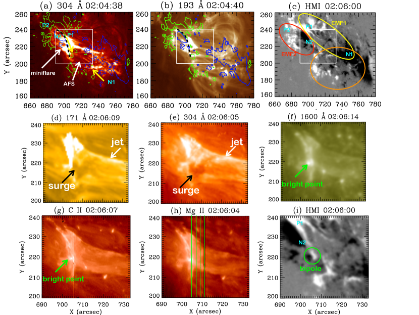
Figure 1: Multi-wavelength observations of the solar jet and surge in different AIA and IRIS wavebands on March 22, 2019. Panels (a-b) show the active region AR 12736 with the mini flare in AIA 304 Å and 193 Å passbands respectively. Panel (c) shows the longitudinal magnetic field configuration observed with HMI consisting of emerging magnetic fields (EMF): EMF1 (P1-N1) and EMF2 (P2-N2) and an earlier EMF encircled respectively by yellow, red, orange ovals. On panels (a-b) the maps are overlaid with the HMI magnetic field contours of strength $\pm$ 300 Gauss, where green contours are for positive and blue for negative magnetic polarity, the magnetic polarity inversion line (PIL) between P1 and N2 along the North-South bright area is indicated by a dashed black line and the dark elongated structures between N1 (yellow arrow) and P1 (AFS), are pointed by a white arrow. The small white square in panels (a-c) shows the FOV for the panels (d to i). Panels (d-f) represent three different AIA channels (171 Å, 304 Å, and 1600 Å), zooming on the jet base in triangle-shape and the surge indicated with white and black arrows respectively. Panels (g-h) are IRIS SJI 1330 Å  and SJI 2796 Å. The four positions of the IRIS slit are shown with green vertical lines in panel (h). Panel (i) is a zoom of the magnetic configuration at the jet base along the PIL between P1 and N2. The polarities P1 and N2 are very much extended along the PIL between them. N2 is continuously sliding along (see magnetic field evolution in an attached animation). In panel (i), the bipole (part of N2-P1) where the reconnection takes place is encircled with green color. This region corresponds to the bright point indicated by a green arrow in panels (f and g). North is up and West is in the right in all the panels.

Broadened Si IV profiles could be also due to the sum of different structures having rapidly changing velocity however it does not seem to be the admitted solution for IBs because they are relatively stable during time, e.g. 15 minutes in the UV bursts studied by Gupta et al. (2015). For other observations of UV bursts the dip in double peaked Si IV line profiles is interpreted to be caused by self absorption mechanism (Yan et al., 2015). Si IV profiles observed in UV bursts vary spatially significantly across the IBs (Yan et al., 2015; Grubecka et al., 2016; Chitta et al., 2017).

With IRIS the chromospheric C II and Mg II lines are frequently observed not only in the UV bursts but also in the quiet chromosphere as well as in solar flares and jets (Leenaarts et al., 2013a; Rathore & Carlsson, 2015). They are optically–thick lines and need a radiative transfer approach to determine the physical quantities of plasma. The Mg II h and k resonance lines in the quiet Sun are formed over a wide range of chromospheric heights. They usually appear as doubly peaked profiles with a central reversal. Simulations in the quiet chromosphere has been carried out by Athay & Skumanich (1968); Milkey & Mihalas (1974); Ayres & Linsky (1976); Uitenbroek (1997); Lemaire et al. (2004); Leenaarts et al. (2013a, b); Pereira et al. (2013). The core of the line is formed just under the transition region (T$<$ 20,000K), the wings at the minimum of temperature (T = 5000 K).

IRIS spectral data allow to make many progresses on the plasma diagnostics in flares. Kerr et al. (2015) and Liu et al. (2015) recently discussed the emission of chromospheric lines as observed in solar flares. They said about these lines that: ”They appeared as redshifted, single-peaked profiles, however some pixels present a net blue asymmetry”. The blue asymmetry can be explained by down-flowing plasma absorbing the red peak emission and not by strong blueshift emission (Berlicki et al., 2005).

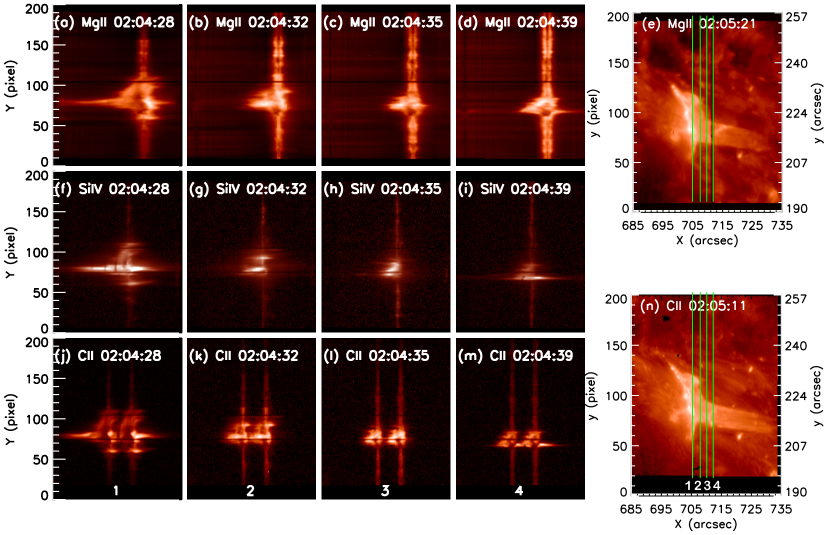
Figure 2: (Left columns 1- 4) IRIS spectra of the Mg II k line at 2796.35 Å (a-d), Si IV 1402.77 Å line (f-i), and C II 1330 Å line (j-m) at the four slit positions of raster 89. (from left to right), slit positions 1, 2, 3, 4 are corresponding to spectra 356, 357,358, 359. The spectra in slit position 1 (column 1) corresponds to the region of the mini flare at the reconnection site. (Right column) SJI 2796 (panel e) and SJI 1330 (panel n) with four green solid vertical lines indicating the four slit positions of the raster. The y axis unit in the SJIs (e and n) is in pixels on the left and arcsec on the right to show the correspondence between spectra and SJIs.

Chromospheric response to intense heating, even in the 1D model, is complicated. The shape of the emission line profiles depends sensitively on the physical conditions of the plasma and its dynamics, in particular the plasma flows that arise at the line core formation heights. They may have symmetrical profiles. Moreover the highest Near Ultraviolet (NUV) continuum enhancements observed in strong flares are most likely because of the Balmer continuum formed by Hydrogen recombination (Kleint et al., 2017) and consequently flares can be assimilated to white light flares, commonly observed in optical continuum where the energy deposit is localized at the minimum temperature region.

The ratio of IRIS transition region lines is also a good diagnostics for the determination of the plasma density in flares (Polito et al., 2016; Dudík et al., 2017). However theoretical simulations showed that this analysis is valid only if there is no self absorption in the transition lines like Si IV and/or if the Si IV lines are not optically thick (Dudík et al., 2017; Kerr et al., 2019). The electron density (N_e) in flare ribbons can be enhanced by two orders of magnitude more than in plage region (N_e $>$ 10 ¹³ cm^-3). For multiple flaring kernels, chromospheric lines show a rapidly evolving double-component structure: an enhanced emission component at rest, and a broad, highly red-shifted component of comparable intensity. Graham et al. (2020) interpreted such observations by beams penetrating very deep in the atmosphere. The red-shifted components migrate from redshifts towards the rest wavelength within 30 seconds. The electron beams would dissipate their energy higher, driving an explosive evaporation, and a counterpart condensation is created as a very dense layer.

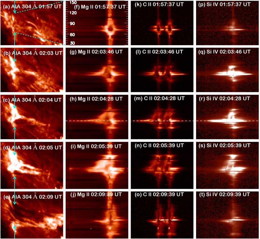
Figure 3: Jet reconnection base (UV burst or mini flare) and jet evolution between 01:57 UT to 02:09 UT (from top to bottom). First column presents the images in AIA 304 Å. Second, third, and last columns show IRIS spectra of the jet reconnection site (UV burst) at slit 1 in the Mg II k 2796.35 Å  line , C II doublet, and in Si IV 1393.76 Å respectively. The vertical cyan arrows and inclined dashed lines (panel (a)) in the first column indicate the position of the slit and the length of the spectra in the three other columns (30 $<$ y (pixel) $<$ 150). The white dashed line in panels (h, m, and r) shows the location for the profiles at y=79 pixel, presented in Fig. 4.

Solar jets are commonly observed with IRIS and the multi wavelength Atomospheric Imaging Assembly (AIA, Lemen et al., 2012) instruments. The characteristics of such jets vary in large parameter ranges: velocity between 100 to 400 km s^-1, length between 50 and 100 Mm (Nisticò et al., 2009; Joshi et al., 2020a). IRIS spectroscopic and imaging observations of jets reveal bidirectional outflows in transition region lines at the base of the jets implying explosive magnetic reconnection processes (Li et al., 2018; Ruan et al., 2019). Bidirectional outflows in the LOS are detected by the extended wings in chromospheric and transition line profiles (Dere et al., 1991; Innes et al., 1997; Tian et al., 2018; Ruan et al., 2019). While they are commonly related to magnetic reconnection, Judge (2015) proposed a different interpretation based on Alfvénic turbulence.

It is not clear the relationship between jets, flares, surges, EBs, and IBs. Young et al. (2018b) reviewed separately all these small transient IRIS phenomena with no real physical link between them. It is useful to be able to provide a scenario where all the pieces of puzzle (using IRIS line profiles of the different ions) can be integrated in a global model of atmosphere for mini flare, jet and IBs.

The present work is focused on a twisted jet and at its base, a flare of B6.7 GOES class (that we call mini flare in this study), which occurred on March 22, 2019 in NOAA AR 12736 around 02:05 UT. The magnetic topology of this region has been studied by Joshi et al. (2020b) (from now we will refer this study as Paper I) and is summarized in Sect. 2. The present paper is mainly focused on the IRIS data in the frame of AIA 304 Å observations. Mg II, Si IV, C II spectra and line profiles at the reconnection site of the jet, are analysed leading to a sketch of dynamical reconnection (Sect. 3). In Sect. 4 we discussed on a possible multi thermal reconnection model with multi layers from very deep layers in the atmosphere, e.g. at the minimum temperature region, to the corona. This is how a sandwich model with stratification of multi layers is proposed to explain the observations during the reconnection. In Sect. 5 we summarized the results and concluded on the multi facets of this mini flare (UV burst and white flare).

Table 1: IRIS observation of NOAA AR 12736 on March 22, 2019.

Location	Time (UT)	Raster	SJI
x=709$\arcsec$	01:43–02:42	FOV:                      6$\arcsec$ $\times$ 62$\arcsec$	FOV: 60$\arcsec$ $\times$ 68$\arcsec$
y=228$\arcsec$		Step size:                     2$\arcsec$	Bandpass: C II 1330 Å,
		Spatial resolution: 0.${\arcsec}$33	Mg II 2796 Å
		Step cadence:        3.6 s	Time cadence: 14 s for each passband

2 Instruments and Observations

2.1 Global evolution of the active region

We report on the observations of a solar twisted jet, a related surge and a mini flare at the jet base in NOAA AR 12736 located at N09 W60 on March 22, 2019.

Figure 1 summarizes the observations obtained with the multi-wavelength filters of AIA and the Helioseismic and Magnetic Imager (HMI, Schou et al., 2012) aboard Solar Dynamics Observatory (SDO, Pesnell et al., 2012), and IRIS. The jet and the mini flare are observed in all the AIA channels covering a wide range of temperatures (10⁵ - 10⁷ K) (animations are attached in AIA 304 Å and 193 Å). Figure 1 (panels a-b) show an example of the mini flare and the jet visible as bright elongated regions in AIA 304 Å (50,000 K) and 193 Å (1.25 MK) filters respectively.

The AR has been formed by successive emerging fluxes during 24 hours before the jet observations. The AR magnetic configuration at the time of the mini flare consists of three emerging magnetic flux (EMF): an earlier one (orange oval) and two very active EMFs: EMF1 (P1-N1) and EMF2 (P2-N2) highlighted by the yellow and the red ovals (Fig. 1 panel (c), see also the animation attached for the magnetic evolution with HMI observations). The contours of the longitudinal magnetic field ($\pm$ 300 Gauss) is overlaid on AIA 304 Å and 193 Å images (Fig. 1 a-b). The polarity inversion line (PIL) between these two EMFs (between P1 and N2 more precisely) is shown by a dashed dark line in panel (a-b). The images of second and third rows in Fig. 1 present a zoom view of the mini flare at the jet base at 02:06:05 UT observed with AIA. In panels (d-f) the jet is seen to develop westwards while the mini flare corresponds to a North-South arch-shape brightening along the PIL and a bright point in its middle (Fig. 1 panel f-g).

In the magnetic field evolution (an animation is also attached as MOV3) the negative polarity N2 is sliding along the positive polarity P1 with possibly reconnection between the two polarities N2-P1 (Fig. 1 panel i). The green circle indicates the small bipole which is the location of the reconnection site at the jet base corresponding to the ‘X’ point. In the bipole formed by the collision of two polarities belonging to two different magnetic systems, strong shear should exist as it was shown in other cases (Dalmasse et al., 2013). There is no visible hot loop in the AIA filters corresponding to this location. After our analysis of the IRIS spectra, we show that the Mg II line profiles at the jet base are similar to the Mg II line profiles in IBs formed in bald patch region where the magnetic field lines are tangent to the solar surface (Zhao et al., 2017). By analogy it suggests that there is a bald patch (BP) region inside the bipole (see section 3.4). It would explain why the bright point is visible at the minimum temperature in the atmosphere e.g in 1700 Å and 1600 Å (Fig. 1 panel f ). This is in the line of the main conclusion of Paper I, where it has been demonstrated that the magnetic reconnection initiating the jet started in a BP current sheet which rapidly became an X-null point current sheet.

In the AIA filters (Fig. 1 panels (a-b)) nearly horizontal dark strands forming arch filament systems (AFSs) are visible in each side of the mini flare. The EUV emission with wavelengths shorter than the hydrogen Lyman and helium discontinuity continuum (912 Å, 504 Å, 228 Å) suffers from the continuum absorption from H I, He I, and He II due to photoionization (Heinzel et al., 2003; Anzer & Heinzel, 2005). Mainly on the West side overlaying EMF1 and the former EMF (orange oval) the AFS structure has an East-West direction. It is common to observe AFS over EMF during the emergence of magnetic flux (Schmieder & Pariat, 2007).

2.2 IRIS observation mode

On March 22, 2019 between 01:43:27 UT and 02:42:30 UT, IRIS was targeting the jet base in the NOAA AR 12736 with a field of view of 60$\arcsec$ $\times$ 68$\arcsec$ centered at x=709$\arcsec$ and y=228$\arcsec$ . When the jet appeared, IRIS acquired slit jaw images (SJIs) in two passbands: SJIs 1330 Å (dominated by the C II lines) and SJI 2796 Å where the emission mainly comes from the Mg II k line.

Details of the IRIS observations are in Table LABEL:table1. The co-alignment between the different IRIS channels was achieved by using the drot_map function of IDL in solar software to correct the differential rotation. Those SJIs were taken at a cadence of 14 sec for each passband.

Simultaneously IRIS performed medium coarse rasters of 4 steps. The raster step size in x is 2$\arcsec$ so each spectral raster spans a field of view of 6$\arcsec$ x 62$\arcsec$ with four positions of the slit. The nominal spatial resolution is 0.$\arcsec$33. During the full observation time it was repeated 250 times. Calibrated level 2 data are used in this study. Dark current subtraction, flat field correction, and geometrical correction have been taken into account in the level 2 data (De Pontieu et al., 2014).

IRIS provides line profiles in Mg II k and h lines (2796.4 Å and 2803.5 Å respectively), Si IV (1393.76 Å, 1402.77 Å) and C II (1334.54 Å, 1335.72 Å) lines along the four slit positions (slit length of 202 pixels equivalent to 62 $\arcsec$). The Mg II h and k lines are formed at chromospheric temperatures, e.g. between 8000 K and 20000 K (De Pontieu et al., 2014; Heinzel et al., 2014; Alissandrakis et al., 2018). C II is formed around T=30,000 K and Si IV around 80,000 K. Many other chromospheric and photospheric lines have been identified in the spectra of the mini flare (see Table LABEL:table2).

Table 2: Identification of the lines in IRIS wavelength ranges of C II, Si IV, and Mg II lines observed in the mini flare at the jet base; (bl) means blended.

Ion	$\lambda$ (Å)		Ion	$\lambda$ (Å)		Ion	$\lambda$ (Å)
C II	1334.54		O IV	1399.776		Mg II triplet	2791.6
C II	1335.72		O IV	1401.163		Mg II k	2796.4
Fe II	1392.817		Si IV	1402.77		Mg II triplet	2797.9
Ni II	1393.33		O IV	1404.806 (bl)			2798.0
Si IV	1393.589		Si IV	1404.85 (bl)		Mg II h	2803.5
Si IV	1393.76		S IV	1406.06

2.3 Mini flare observed with AIA and IRIS

An example of IRIS SJIs in 1330 Å and 2796 Å  is presented in Fig. 1 (g-h). West is on the right and East on the left in all the panels with images. The FOV of IRIS SJIs includes the mini flare (bright point in panels (f-g)) and a part of the wide jet base. The bright point is considered as as the reconnection site (or ‘X’ point) at the jet base. The four positions of the slit scanned the mini flare site around x= 705$\arcsec$ and y = 220$\arcsec$ and the arch-shape brightening at the base of the jet (see in panel (h)). Globally the structures visible in IRIS SJIs are similar to those in AIA 304 Å (50,000 K). The FOV of IRIS has been shifted by 4 arcsec in x axis and 3 arcsec in y axis to be co-aligned with AIA coordinates.

In AIA 304 Å  between 02:04:09 UT to 02:06:09 UT we see that the jet base has a triangular shape. Between the two external sides of the jet’s triangular base there are two slightly bright patches in an East-West direction. In C II observations (an animation is attached as MOV4) we can follow the formation of small kernels at 02:04:28 UT, 02:05:25 UT, 02:05:39 UT, and 02:06:07 UT, travelling from one side to the other side of the triangle following these bright patches (from east to west). In AIA 304 Å images, the development of the surge is well visible in between 02:04 and 02:07 UT (Fig. 1 panel (e) at 02:06:05 UT). However, the surge is not so well visible in IRIS SJIs 1330 Å and 2796 Å  taken at the corresponding times (panels g-h). This can be explained because the absorption of the UV emission is only efficient for lines with wavelengths below the hydrogen Lyman continuum limit ($\lambda$ $<$ 912 Å) (Schmieder et al., 2004). Moreover, the non-visibility of the surge can be due to the large wavelength ranges of the IRIS SJIs filters where the full line profiles are integrated and the line emission in the jet was not strong enough.

3 Spectroscopic analysis

To process the IRIS Mg II h and k data, we used the spatial and wavelength information in the header of the IRIS level-2 data and derived the rest wavelengths of the Mg II k 2796.35 (4) Å, and Mg II h 2803.52 (6) Å  from the reversal positions of the averaged spectra at the disk. For C II and Si IV lines the zero velocity is defined in a similar way (see Table LABEL:table2 for the rest wavelengths used in the present work).

3.1 IRIS spectra of mini flare

We show one example of spectroscopic data obtained between 02:04:28 UT and 02:04:39 UT with the four slit positions 1, 2, 3, 4 for the three different elements Mg II, C II, and Si IV (Fig. 2). The correspondence between pixels along the slit and arcsecs in SJIs is shown as y coordinates of the SJIs (Figure 2 panels e and n). The slit position 1 shown in panel (n) crosses the bright zone between 60 to 105 pixels (around 210-230 arcsec) corresponding to the jet base. In the middle of the zone, the brightest point along the slit is the reconnection site (y $\approx$ pixel 79- 80 corresponding to the position ‘X’ (705$\arcsec$, 220$\arcsec$) in Figs. 1 (g) and 2 (e,n)). These spectra observed around 02:04 UT (panels a-m) correspond to the onset of the mini flare,

At the reconnection site the spectra shows very complex structures that we will analyse in the next sections. We note that in all the slit positions 1-4, similar features are shown, but they are more pronounced in the slit position 1, which seems to be exactly at the reconnection site for this time. We will mainly restrict our study to the slit position 1. It is not really possible to reconstruct an adequate spectroheliogram image with only four positions distant in x of 2$\arcsec$ each.

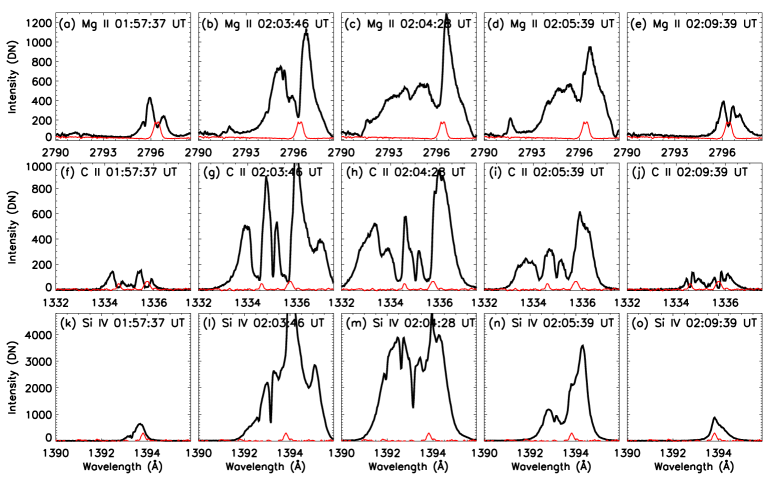
Figure 4: (from left to right) Evolution of jet reconnection site (UV burst) between 01:57 UT and 02:09 UT through the profiles of the Mg II k (a to e), C II (f to j), and Si IV 1394 (k to o) lines observed in slit 1 at y = 79 pixel. The location of the y point in the different spectras is shown in Fig. 3 with a white dashed line.The considered spectra data are the same as those used for Figure 3. The small red profile in each panel is the reference profile. The reference profiles of C II and Si IV lines are raised by a factor of 5 and 20 respectively.

3.2 Time evolution of IRIS spectra of mini flare

We note in Sect. 2.3 that AIA 304 Å images have a better contrast than the IRIS SJIs to show the cool structures visible by absorption. Therefore we co-align carefully the images in AIA 304 Å with the IRIS SJIs in order to indicate exactly the position of each pixel of the slit in the AIA 304 Å  images to be able to discuss the evolution of the structures visible in the 304 Å  images jointly with the spectra shape of IRIS lines using both coordinates the pixels along the slit and the AIA coordinates.The evolution of the structures visible in AIA 304 Å images: mini flare, jet and surge are summarized in five different times in Figure 3, corresponding to: pre reconnection time (first row), reconnection times (second and third rows), jet base extension (third row), after reconnection time (fifth row) (also see the movie in AIA 304 Å animation attached MOV1). Between the two vertical blue arrows in the AIA images (left column), a section of slit at position 1 is located. The right columns present the spectra in this section for the three elements Mg II, C II and Si IV. Table LABEL:table4 gives a detail about the characteristics of these typical profiles in the four slit positions during the different phases of the jet time observations. They are changing very fast and it is rather complicated to analyse all of them. We will nevertheless focus on the profiles which are important for understanding the reconnection process in Sects. 3.3 to 3.6 and be able to proceed to a dynamical model of reconnection (Sect. 14).

3.3 Characteristics of the spectra: spatio-temporal analysis of IRIS spectra

For each IRIS spectra shown in Fig. 3 we select the pixel 79 corresponding to the reconnection site and draw the line profile of the three elements for the five times (see Fig. 4). The line profiles help to interpret the nature and evolution of the structures during the different phases of the reconnection. We focus our analysis of Mg II and C II chromospheric lines in the following subsections during the three phases of the jet reconnection. Then we analyse in details the line profiles of the three elements during the reconnection times (Sect. 3.4).

3.3.1 Pre reconnection time

Around 01:57 UT in AIA 304 Å image, tiny vertical bright areas along the inversion line are visible (see panel (a1) in Fig. 3). The corresponding C II and Mg II spectra show very large central dip which could represent the presence of cool material at rest which absorbs the incident radiation (Fig. 3 panels (b1 and c1)) and the corresponding line profiles in Fig. 4 panels (a and f).

The Mg II k and C II line profiles at this position and around (pixels= 70, 76, 79) are presented again but with a zoom and with the x-axis in Dopplershift units in km s^-1 (Fig. 5). They are very broad with a central dip (FWHM more than 1 Å  which corresponds to +/-50 km/s) while the peaks of the Mg II and C II lines are equally distant (100 km s^-1). The central dip would imply that cool material absorbed the incident radiation more or less at the rest. Such cool material could be due to parts of arch filaments trapped in the magnetic field lines between the two EMFs (EMF1 and EMF2) in the vicinity of the bright point region before the reconnection.

3.3.2 During the reconnection time

Around 02:03 - 02:05 UT the mini flare (UV burst at the ‘X’ point) starts in the middle of this bright area with the onset of the jet ejection (Fig. 3 with 304 Å images in panels (b,c,d), Mg II spectra in panels (g,h,i) and C II spectra in panels (l,m,n)) and their corresponding line profiles in Fig. 4 panels (b,c,d and g,h,i). The bright jet is obscured by a surge, a set of dark (cool) materials in front of it; both the jet and the surge are extending toward the West at the same time. In AIA 304 Å  image at 02:05 UT the jet is extended along two bright branches with a dark area in between. During this time the spectra show very broad blue wings along the slit in the same zone $\pm$ 10 arcsec around y=220$\arcsec$. At y= 79 pixel (approximately at 220$\arcsec$), the profiles in all the lines are the most extended (Fig. 4 panels (b,c,d and g,h,i)). We notice that the spectra along the slit show a tilt at the northern bright branch (Fig. 3 panels i,n), which could indicate some rotational motion there (see Sect. 3.6 for more details). The wavelength positions of the dark absorption core of the Mg II and C II line profiles along the slit show a clear zigzag pattern of the blue and red shifts which could correspond to cool plasma motion with different velocities along the slit. In the next sections (Sects. 3.4 and 3.5) we analyse the profiles of the three lines to obtain quantitative values of the Dopplershifts of the plasma in the reconnection zone of the jet.

3.3.3 After reconnection time

At 02:09 UT, long dark East-West filament structures in the North of the reconnection site are observed in the 304 Å images (see Fig. 3 (e)). Their corresponding spectra show a dark core and weak emission in the red wings all along the slit (y(pixel)=70-105) which could correspond to cool plasma absorbing the red peak emission of the jet. This cool plasma may be plasma of the surge or to the arch filament system going away of the observer with Dopplershifts of less than 30 km s^-1 (Fig. 3 (j and o)). We note an enhancement of the continuum emission close to the Mg II lines which could correspond to enhancement of the Balmer continuum like in white light flares (Fig. 3 panel i) (Heinzel & Kleint, 2014).

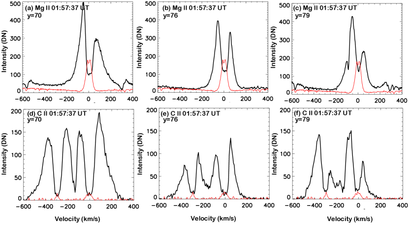
Figure 5: Comparison of the profiles of Mg II k (top row) and the two C II (bottom row) lines in three pixels along the slit at the position of the UV burst at 01:57:37 UT before the burst (Fig. 3 f). The x axis unit is velocity to compare the shift of the peaks of the Mg II and C II lines. We note the same large distance between the two peaks of the Mg II and C II lines, which could be due to the presence of cool material in the region of the reconnection before the reconnection. The red profiles are reference profiles, which were used to determine the rest wavelengths.

3.4 UV burst in ‘X’ point- large blueshift

The IRIS slit at position 1 crosses the mini flare (UV burst at ‘X’ point) so that the spectra along the slit bring many information about the dynamics of the UV burst as explained in the previous section (Sect. 3.3) and in Fig. 3. Figure 4 shows the evolution of the UV burst using the three lines (Mg II, C II, and Si IV) profiles for y(pixel)=79 (220$\arcsec$) with a time scale of one minute. The profiles change very fast on this time scale. We analyse these profiles at each time in order to derive the characteristics (velocity and temperature) of structures which are integrated along the LOS.

At 02:03:46 UT in very localized pixels inside the burst Mg II, C II and Si IV profiles have more or less symmetrical profiles with high peaks with extended blue and red wings ($\pm$ 200 km s^-1) (Fig. 4 panels b, g, i and in Annex: Fig. 16 a and 17). With such extended wing profiles in a few pixels we may think of bilateral outflows of reconnection (Ruan et al., 2019). Such outflows with super Alfvénic speeds were observed in a direction perpendicular to the jet initiated by the reconnection like in our observations.

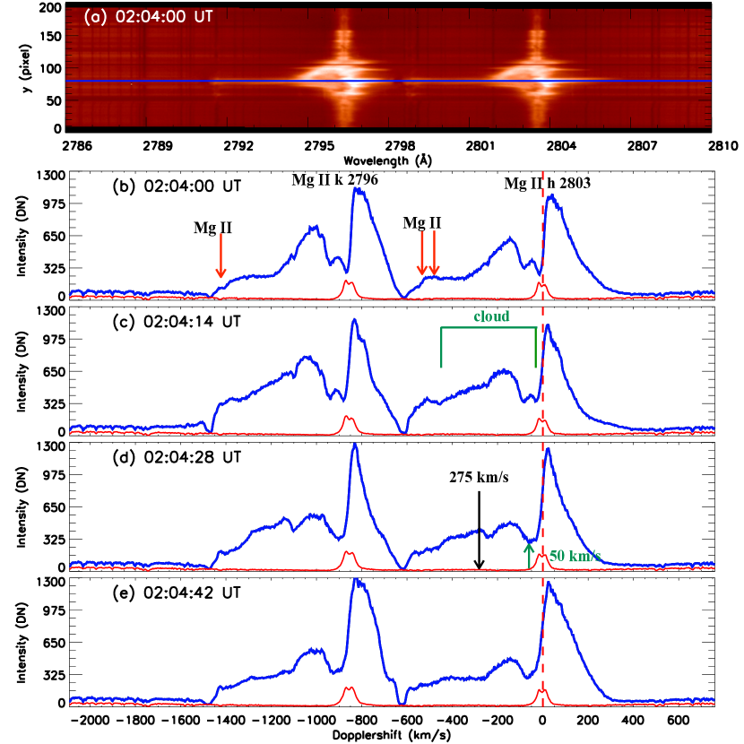
Figure 6: (a) Mg II spectra at 02:04:00 UT along the slit position 1 before the UV burst (Fig. 3 g). Panels (b-e) from top to bottom: evolution of the Mg II k and h line profiles (for y = 79 pixel in panel (a)) showed by a profile every 14 sec during less than one minute time (02:04:00-02:04:57 UT) (Fig. 3 h). The emission of the Mg II triplet line profiles–one at 2791.6 Å and other two at 2799 Å  are indicated by red arrows in panel (b). The horizontal green brace points the low intensity value of the Mg II blue peak, signature of the possible presence of an absorbing (red arrow in panel d) and emitting radiation cloud (black arrow in panel d) along the line-of-sight. The reference profiles are shown in red. The vertical red dashed lines in panels (b-e) show the position of rest wavelength at 2803.6 Å. The wavelength range in panel (a) and (b-e) is same in wavelength unit for panel (a) and the corresponding Dopplershift unit in panel (e).

For the time of reconnection around 02:04:28 UT, Mg II, Si IV and C II line spectra are presented for the four slit positions (Fig. 4). The profiles at this time at y=79 pixel exhibit a high peak of emission with strong blue shift extended wing (see third column (panels c,h,m) in Fig. 4) although the evolution of the profiles are shown with a low cadence. In Figures 6 and 7 we show the details of the fast evolution of the UV burst between 02:04:14 UT and 02:04:28 UT taking advantage of the high cadence of IRIS (14 sec).

The Mg II profiles of the UV burst during this time scale did not evolve drastically, contrary to the Si IV profiles in the same time interval. The Si IV profiles are very broad during the UV burst maximum with a FWHM of the order of 4 Å (Fig…7. A few seconds later at 02:04:57 UT the Si IV profiles consist only of one peak with a FWHM of 1 Å  and an intensity increasing about a factor of 100.

We analyse first the Mg II profiles of the mini flare (UV burst) to understand the composition and the dynamics of the plasma along the LOS. The zero velocity is defined, as we explained earlier, by the dip in the reverse profile of Mg II line profile observed in the chromosphere. The Mg II profiles are also very broad with a FWHM of the order of 5 Å  and asymmetric with a high red peak and a very extended blue wing (Fig. 6). The blue peak is much lowered compared to the red one. This characteristic of the profiles can be produced by the absorption of the blue peak emission by a cloud centered around 50 km s^-1. In the far blue wing an emission is detected until -5 Å, which might come from a second cloud centered around a higher value (intuitively determined around - 275 km s^-1) and the emission of the Mg II triplet at 2797.9 and 2798 Å which are effectively at -5 Å from Mg II h. All the Mg II triplet lines have been identified in the spectra (Table 2).

The profiles of Mg II, C II, Si IV lines at the UV burst plotted in Dopplershift units relative to the rest wavelength show similar velocities, which indicates that they correspond to real plasma moving with high flow speed (see Fig. 8). Although the extended blue wings could also be interpreted as due to a gradient of velocity inside the cloud along the LOS instead of a moving cloud. In the next section we apply a cloud model technique to have quantitative results.

3.5 Cloud Model Method for Mg II lines

Cloud model method was first introduced by Beckers (1964) for understanding asymmetric line profiles in the chromosphere. The structure overlying the chromosphere is defined by four constant parameters: optical thickness, source function, Doppler width and radial velocity. Moreover, Mein & Mein (1988) developed the cloud method by considering non constant source function and velocity gradients. Therefore this technique was applied for different structures with large velocities, mainly observed in the H$\alpha$ line, e.g. post flare loops (Gu et al., 1992; Heinzel et al., 1992), spicules on the disk (Heinzel & Schmieder, 1994), and atmospheric structures in the quiet-Sun (Mein et al., 1996; Chae et al., 2020), even using multi clouds (Gu et al. (1996); Dun et al. (2000), see review by Tziotziou (2007)). This new development allows to derive dynamical models in the chromosphere (Heinzel et al., 1999). This technique is valid for a chromospheric structure with a large discontinuity (e.g. a high radial velocity), overlying the chromosphere along the LOS.

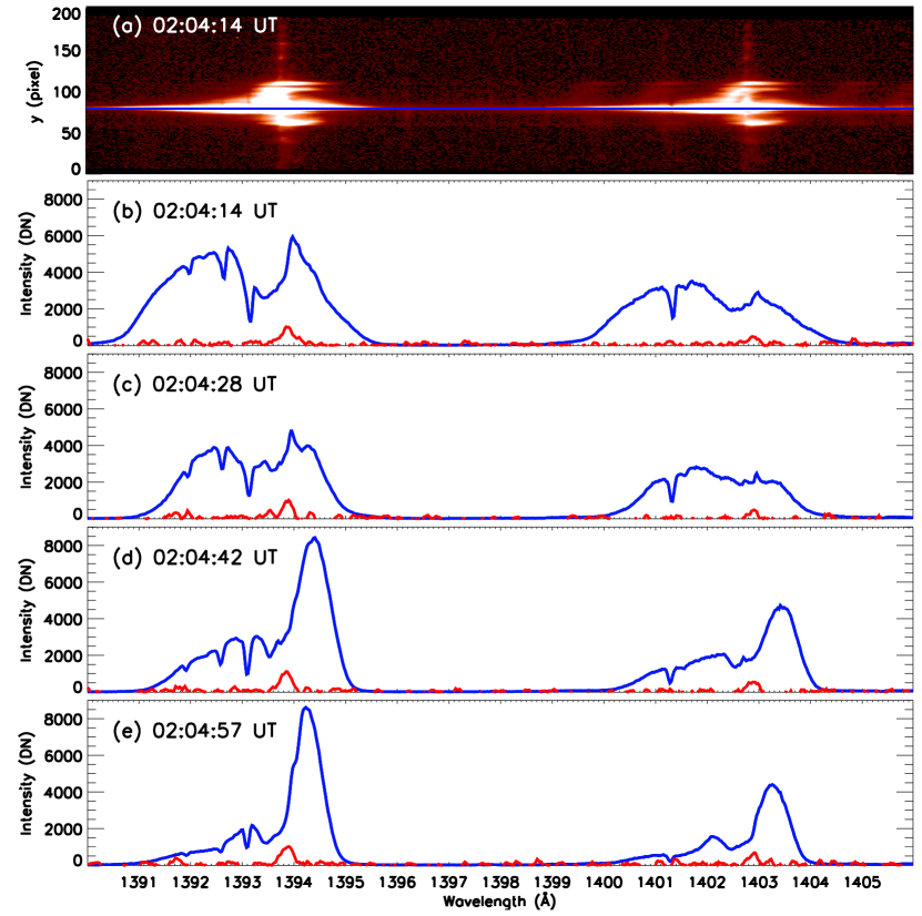
Figure 7: (a) Si IV spectra at 02:04:14 UT at the start of the UV burst (Fig. 3 a). Panels (b-e): from top to bottom: fast evolution during less than one minute, one Si IV profile every 14 s at slit position 1 between 02:04:14 UT and 02:04:57 UT. The profiles from panel (b-e) are taken at y(pixel) = 79, shown as blue horizontal line in panel (a). The reference profiles are shown in red. .

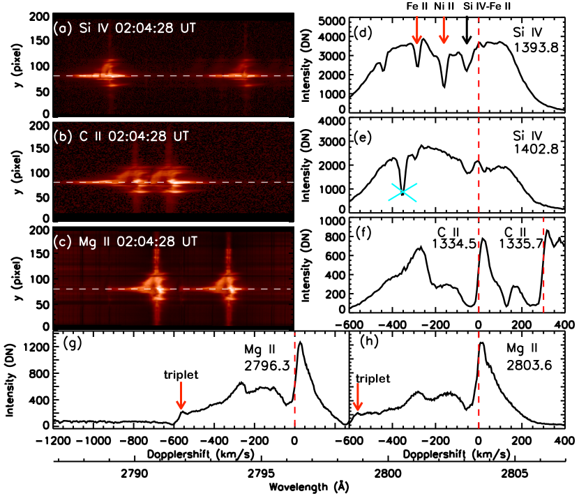
Figure 8: Spectra of the jet base (UV burst) showing the extended blue wing of Si IV line (panel (a)), C II line (panel (b)) and Mg II line (panel (c)) at 02:04:28 UT (Fig. 2 left column), the white horizontal dashed lines in these three panels indicate the position where the profiles are drawn in panels (d-h). In panels (d-h), the horizontal wavelength axis is shown as Dopplershift relative to the rest wavelength in each window. The Doppler-shift scale in all panels is the same for the comparison of the Dopplershifts in three element lines. We note the presence of dips in the Si IV profiles corresponding to absorption of chromospheric lines (Ni II 1393.33 Å  and Fe II 1393.589 Å) indicated by red arrows in (d). The black arrow in panel (d) indicates a dip due to self-absorption of Si IV line blended by a Fe II line. The cyan cross in panel (e) points a dip with missing data in the spectra. The dashed vertical red lines indicate the zero velocity. The red arrows in panels (g-h) indicate the emission of Mg II triplet lines.

Recently Tei et al. (2018) applied the cloud model technique with constant source functions to the Mg II lines which present complex profiles because of their central reversal. Considering multi clouds, Mg II complex profiles of off-limb spicules were successfully fitted (Tei et al., 2020).

Cloud model technique applied to Mg II lines allows us to unveil the existence of moving clouds over the chromosphere. For the present analysis, this is how during the peak phase of the reconnection two clouds overlying the region of reconnection are considered to fit the asymmetric Mg II profiles observed in the UV burst region. Mg II asymmetric line profiles are assumed to be the result of the presence of two overlapping clouds c1 and c2 located above a background atmosphere along the LOS. We suppose the background atmosphere is symmetric with high peaks in the Mg II lines. We consider a situation where the cloud c2 is located above the cloud c1 along the LOS. Assumptions relative to the two clouds are as follow;

1. The absorption profile of a cloud has a Gaussian shape.

2. The two clouds have generally different physical properties.

3. The source function, the LOS velocity, the temperature, the turbulent velocity in each cloud are independent of depth (constant in the cloud).

The first assumption concerning the absorption profile shape described by a Gaussian function is defended by the following argument. We are mainly interested in the Doppler-shifted feature and we derive its velocity using the standard cloud model. In the center of this Doppler feature, the line absorption profile is very well described by the Gaussian function (the Voigt function is approximately Gaussian in the line core and Lorentzian in the wings) and thus we use it for simplicity.

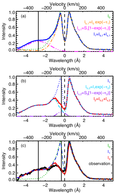
Figure 9: Two-cloud model calculation of the Mg II k line profile at 02:04:28 UT for pixel y=79 (Fig. 6 d). We consider a situation where the cloud c2 is located above the cloud c1 along the LOS. (a) Detail of the $I_{1}$ profile. Dotted (green) line shows $I_{0}$, the background intensity profile (symmetric) made from the red-side of the observed intensity profile (part of the mini flare symmetrical profile). Dot-dashed (orange) line shows $I_{b,1}\equiv I_{0}{\rm e}^{-\tau_{1}}$, the background intensity attenuated by the cloud c1. Dot-dot-dot-dashed (pink) line shows $I_{s,1}\equiv S_{1}[1-{\rm e}^{-\tau_{1}}]$, the emission from the cloud c1. Solid (blue) line shows $I_{1}=I_{b,1}+I_{s,1}$, the resulting intensity profile when there are only the background atmosphere and the cloud c1 along the LOS. (b) Detail of the $I_{2}$ profile. Dotted (blue) line shows $I_{1}$, the intensity from the background and the cloud c1 (as ”background” intensity profile for the cloud c2). Dot-dashed (light blue) line shows $I_{b,2}\equiv I_{1}{\rm e}^{-\tau_{2}}$, the intensity from the background and the cloud c1 attenuated by the cloud c2. Dot-dot-dot-dashed (purple) line shows $I_{s,2}\equiv S_{2}[1-{\rm e}^{-\tau_{2}}]$, the emission from the cloud c2. Solid (red) line shows $I_{2}=I_{b,2}+I_{s,2}$, the resulting (modeled) intensity profile when there are the background atmosphere, the cloud c1, and the cloud c2. (c) Comparison of observed (solid, black) and modeled (solid, red) profiles. The background profile $I_{0}$ (dotted, green) and the profile $I_{1}$ (dashed, blue) are also shown for comparison. The vertical solid black lines in each panel show the LOS velocity values of the considered clouds.

The total observed intensity $I_{m}(\Delta\lambda)$ emitted, when there is one cloud (m=1) or there are two clouds (m=2) on the background atmosphere of intensity $I_{0}(\Delta\lambda)$ along the LOS, is given by the relation

$$I_{m}(\Delta\lambda)=I_{m-1}(\Delta\lambda){\rm e}^{-\tau_{m}(\Delta\lambda)}+S_{m}[1-{\rm e}^{-\tau_{m}(\Delta\lambda)}],$$ (1)

where $S_{m}$ is constant the source function and

$$\tau_{m}(\Delta\lambda)\equiv\tau_{0,m}\exp\left[-\left(\frac{\Delta\lambda-\Delta\lambda_{{\rm LOS},m}}{\Delta\lambda_{{\rm D},m}}\right)^{2}\right]$$ (2)

is the optical thickness of the cloud c1 (m=1 case) or c2 (m=2 case) with the Doppler width

$$\Delta\lambda_{D,m}\equiv\frac{\lambda_{0}}{c}\sqrt{\frac{2k_{\rm B}T_{m}}{m_{\rm Mg}}+V_{{\rm turb},m}^{2}}.$$ (3)

Here, $\Delta\lambda=\lambda-\lambda_{0}$ is the difference between the wavelength, $\lambda$, and the rest wavelength of the Mg II line considered, $\Delta\lambda_{{\rm LOS},m}\equiv\lambda_{0}V_{{\rm LOS},m}/c$ is the shift of wavelength corresponding to the LOS velocity of the cloud of number m, $V_{{\rm LOS},m}$ ($c$ is the light speed); $T_{m}$ and $V_{{\rm turb},m}$ are the temperature and the turbulent velocity of the cloud of number m, respectively; $k_{\rm B}$ is the Boltzmann constant; $m_{\rm Mg}$ is the atomic mass of magnesium. Combining the equation (1) of $m=1$ and the one of $m=2$, the total observed intensity $I_{2}(\Delta\lambda)$ emitted by two clouds is given by the relation

$$I_{2}(\Delta\lambda)=I_{0}(\Delta\lambda){\rm e}^{-\tau_{1}(\Delta\lambda)}{\rm e}^{-\tau_{2}(\Delta\lambda)}+S_{1}[1-{\rm e}^{-\tau_{1}(\Delta\lambda)}]{\rm e}^{-\tau_{2}(\Delta\lambda)}$$ (4)

$$+S_{2}[1-{\rm e}^{-\tau_{2}(\Delta\lambda)}].$$

In the present work, we adopt $T_{1}=T_{2}=10^{4}$ K since the cloud temperatures do not affect the result as long as we use a temperature lower than 20000 K at which Mg II is ionized. This is because Mg atom is relatively heavy and the thermal width is small compared to the non-thermal velocity in this situation. For the background intensity, $I_{0}(\Delta\lambda)$, we use a symmetric line profile constructed from the red-side of the observed profile, as done by Tei et al. (2018). In addition, $\alpha_{m}$ is defined as the ratio of the source function of the cloud of number m to the background intensity at the line center [$\alpha_{m}\equiv S_{m}/I_{0}(\Delta\lambda=0)$]. We consider a situation where a low velocity component is in the foreground (c2) along the LOS in order to lower the peak intensity as it is observed. Figure 9 shows the result of a two–cloud model fitting. The values of the free parameters are summarized in Table 3. Two clouds have been detected, one with strong blueshifts (-290 km s^-1) and the other with a large optical thickness but lower blueshift (-36 km s^-1); these values are not far from our approximate estimation (Sect. 3.4). Note that here the radiative transfer is completely treated under the above conditions. The turbulent velocity derived for the cloud c1 is large (150 km s^-1). This could correspond to the existence of a large velocity gradient inside the cloud, which has not be considered in the assumptions where on the contrary all the parameters are constant. On the other hand, we may note that the assumption of a symmetrical Mg II profile background for the flare does not influence the fast cloud existence, since the wavelength range of this component is very far in the wing (see Fig. 9).

Table 3: Results of two-cloud modeling (c1 and c2)

Cloud c1
$\alpha_{1}$	$\tau_{0,1}$	$V_{{\rm LOS},1}$	$V_{{\rm turb},1}$
1.6	0.99	$-$290 km s-1	150 km s-1
Cloud c2
$\alpha_{2}$	$\tau_{0,2}$	$V_{{\rm LOS},2}$	$V_{{\rm turb},2}$
0.5	1.6	$-$36 km s-1	50 km s-1

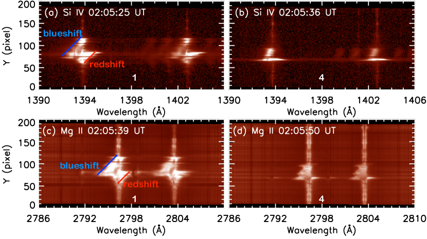
Figure 10: Tilt observed in the Si IV and Mg II spectra during the GOES flare time at slit positions 1 and 4, distant of 6 arcsec (panels a-b for Si IV lines, panels c-d for Mg II lines) (see Fig. 3 panels d, i, s). The blue and redshifts are shown with the solid lines in the spectra of Si and Mg at slit position 1.

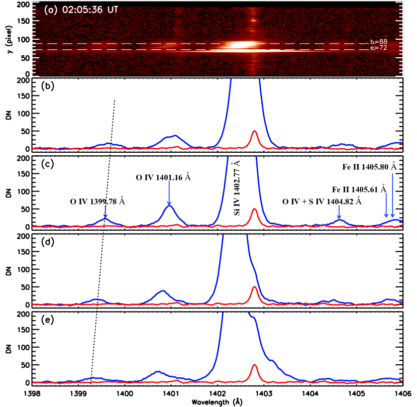
Figure 11: Si IV profiles in slit position 4 at 02:05:36 UT for pixels y = 72 (panel e), y = 76 (panel d), y = 82 (panel c), and y = 88 (panel b). The positions of these pixels lie between the two dashed lines in panel (a). The vertical dashed line in panels (b-e) represents the tilt of the spectra. In position 4 the profiles are mainly blueshifted above a pixel with bilateral flows. The nominal wavelengths of each identified line are written on the top of the lines and are listed in Table LABEL:table2. Reference profile is drawn in each panel in red.

3.6 Spectral tilt profiles

Spectra of the Mg II, C II, and Si IV lines show a spectral tilt at 02:05:39 UT (Fig. 3 panels (i,n,s)). Figure 10 details the spectra of Mg II and Si IV lines for different times 02:05:25 UT and 02:05:39 UT in two slit positions distant of 6 arcsec. The tilt is visible in these two positions, the profiles have dominant red wings in the southern part of the brightening (y(pixel) = 50 to 79), they become roughly symmetric in the middle of the brightening (y = 79) with large extended blue wing nevertheless and show dominant blue wings in the northern part with decreasing blueshifts until being symmetrical profiles (y = 79 to 120). The tilt is well visible in O IV lines, lines in emission identified in the vicinity of Si IV 1402.77 Å  (see Table LABEL:table2 and Fig. 11). We could quantify the displacement of the line according to the position along the slit.

These types of spectra are well known and are typically associated with twist (De Pontieu et al., 2014) or rotation (Rompolt, 1975; Curdt et al., 2012) or the presence of plasma in helical structures (Li et al., 2014). The tilt observed in our spectra can be explained by the presence of an helical structure at the base during the reconnection process due to transfer of twist from a flux rope in the vicinity of the jet, to the jet (Paper I).

3.7 Sketch of the dynamical plasma

We propose a sketch to explain the dynamics of the plasma during the reconnection (Fig. 14). We draw the field lines in solid black lines, the flow directions are indicated with blue or red arrows, with solid thick arrows for blueshifts or redshifts. Before the jet onset (panel a) the magnetic topology of the region consists of two emerging flux: EMF1 and EMF2 overlaid by AFS (see Sect. 2.1). Between EMF1 and EMF2 the bipole (P1-N2) is located, where the reconnection takes place. Just before the reconnection (panel b), there is the formation of a suspected bald patch region in the middle of the bipole with cool plasma trapped inside (see Sect. 3.2). At the time of reconnection (panel c) cool plasma clouds are ejected with strong blueshifts (see Sect. 3.3). As the region is located at W 60, the clouds with blueshifts are in fact ejected over the emerging flux EMF2. At the same time the bald patch is transformed in an ‘X’ null-point current-sheet with bilateral outflows (panel c). Simultaneously there is the ejections of the jet and surge on the right side of the reconnection site over EMF1 (panel d). After the reconnection long AFS and hot loops are formed overlying the region (panel e). This sketch is in the line of the cartoon proposed in Paper I for explaining the reconnection in a X-current sheet.

4 Multi temperature layers

4.1 Presence of cool material over hot atmosphere

During the reconnection time (around 02:04 UT) the IRIS spectra in the mini flare show the presence of cool material over hot plasma like in IBs (Sect. 3.3). This is how the Mg II large extended blueshift profiles have been interpreted by the existence of two cool clouds over the reconnection site at the time of the reconnection. One part of the trapped cool material could be ejected with a low velocity while the other part is ejected with a fast upward velocity during approximately one minute. Cool material is propelled to a distance of 20,000 km along the LOS in one minute (300 km s^-1 $\times$ 60 sec). Moreover the large dark dip in the Mg II line centers at this time could be considered as the cool plasma of the surge which exhibits low Dopplershifts but high transverse velocity (see also the animation attached as MOV1 in AIA 304 Å).

The presence of such cool plasma over the heated atmosphere at the reconnection site is also confirmed by the presence of chromospheric lines striping the Si IV profiles. Si IV 1393.8 Å  profiles in the UV burst reveal that the presence of absorption lines from singly ionized species (Fe II and Ni II) (Figs. 8d, 17e and Table LABEL:table2). The presence of such lines superimposed on emission lines implies that cool chromospheric material is stacked on top of hot material. The cool material would come from the bald patch region when the magnetic field lines were tangent to the solar surface at the photosphere (Fig. 14 panel b). During the bald patch reconnection cool material is ejected with more or less fast flows as we have shown in the explanation of the Mg II profiles. The wavelengths of these Fe II and Ni II lines are located at around 0.5 to 1 Å far from the Si IV line center. Therefore only when the Si IV line profiles are broad enough with extended wings, these chromospheric lines are shown themselves in absorption. It has been already observed in the IBs (Peter et al., 2014) and IRIS UV bursts (Yan et al., 2015).

Moreover at the time of the mini flare (02:04:28 UT) a narrow dip in the profile of Si IV at its rest wavelength is observed, blended by Fe II line (Figure 8). It could be due multi-component flows like in the IBs (Peter et al., 2014). If that would be the case, then one would expect the line profile to be composed of two or more Gaussians at different Dopplershifts representing the different flow components. However it looks not to be the case and the dip is deeper for the strongest Si IV line 1394 Å, and the dip is always at the rest wavelength. Therefore this dip in Si IV could be the signature of opacity effects as in the UV burst presented in Yan et al. (2015). The former authors show similar profiles of Si IV with self absorption and with chromospheric lines visible as absorption lines. They explain these profiles by the superposition of different structures, in the deep atmosphere the reconnection leads to a significantly enhanced brightness and width of Si IV, the light passes through the overlaying cool structures where Ni II leads to absorption. Higher up there is emission of Si IV in overlying cool loops which lead to narrow self-absorption of Si IV. This scenario is possible in our observations.

In the UV burst bilateral outflows and expelled clouds with super Alfvénic flows of the order 200 km s^-1 have been observed in Mg II and Si IV (Sect. 3.4). These profiles are similar to those of IBs found by Peter et al. (2014); Grubecka et al. (2016). However, we detected also O IV lines in the vicinity of Si IV 1393.76 Å (Table LABEL:table2 and Fig. 11). O IV are forbidden lines formed just below 0.2 MK. Our UV burst is definitively not exactly an IB where O IV lines were not detected (Peter et al., 2014) and did not support the long debate about the temperature of the formation on Si IV line. Si IV could be out of ionization equilibrium in high velocity flow plasma and the nominal formation temperature of Si IV could be in fact lower than 80,000 K (Dudík et al., 2014; Nóbrega-Siverio et al., 2018). However when we observe simultaneously O IV line emission as well as Si IV which is also formed at transition region temperatures it confirms that the plasma is heated and Si IV is not at chromospheric temperature. In fact AIA observations showed the mini flare in its hotter filters until 10⁷ K with 211 Å  filter.

4.2 Optical thickness and the electron density

Using IRIS transition region lines (O IV, S IV and Si IV) electron density may be computed (Dudík et al., 2017; Polito et al., 2016; Young et al., 2018a). We note that in the spectra corresponding to the reconnection site at the reconnection time, O IV lines are detected, even the emission is relatively weak (Figs. 7, 10 top panels and 11). Si IV line profiles vary drastically according to time or location as we have already mentioned in Sect. 3.4. The great variety of shapes of profiles of the Si IV lines rises a question about the variations of the optical thickness throughout the observed mini-flare area. For this investigation, we employ the method involving the intensity ratio of the Si IV 1393.75 Å and 1402.77 Å resonance lines (Del Zanna et al., 2002; Kerr et al., 2019). Since a long time this technique exists for stars to determine the amount of opacity in the Si IV lines and is very powerful for providing the physical dimensions of the scattering layer (Mathioudakis et al., 1999).

For computing the intensity Si IV ratio we select two observing times : one time during reconnection (02:04:28 UT) with slit 1 at the reconnection location (Fig. 7), and the other time at one minute later (02:05:36 UT) in slit 4 at the jet base (6″away the reconnection point).

4.2.1 Si IV integrated intensity

During the reconnection phase in slit position 1 at 02:04:28 UT, the extended profiles of the Si IV resonance lines were obtained by summing the intensities observed at the different wavelengths throughout the profiles (Fig.7). We note that the absorption features were excluded from the analysis. However the Si IV 1402 Å  are so wide (4 Å), overlying other transition region lines (O IV lines). We are not able to remove the contribution of these lines from the integrated Si IV line intensity values. Based on the relatively-low intensities of these blending lines, we do not expect the uncertainty of this method to exceed 10%.

Away from the reconnection region, in slit position 4 at 02:05:36 UT, we compute the line integrated intensities by fitting the observed profiles with Gaussian functions using the xcfit.pro fitting routine. Typically, two Gaussian functions were needed to fit each line profile of Si IV, in the mini-flare area between y = 76 and 88. The two Gaussian functions are separated by up to $\approx$0.4 Å, one function has a narrow Full Width half maximum (FWHM) and the other one an extended FWHM but with a lower intensity (Dudík et al., 2017). The two Si IV line profiles showed similar asymmetries. Particularly exceptional profiles of both lines were observed at y $\approx$80, where the ‘bumps’ in line red wings were considerably weaker. Based on this, we suggest that the bumps present in the profiles do not originate in blends, but in the motion of the emitting plasma. To check this assumption, we calculated synthetic spectra using CHIANTI v7.1 (Dere et al., 1997; Landi et al., 2013) for log($N_{\text{e}}$ [cm^-3]) = 11 (see below), flare DEM. Even though we found several lines blending both lines of Si IV, their contributions were found to be negligible.

4.2.2 Si IV ratio

The ratios of the Si IV 1393.75 Å and 1402.77 Å resonance lines are shown in Fig. 12. There, the diamonds indicate the measured ratios at different positions along the slit. They were color-coded in order to distinguish between the ratios measured in (blue) and away (red) from the reconnection region.

For optically thin plasma, this ratio should be equal to 2 (Del Zanna et al., 2002; Kerr et al., 2019), which we indicated using grey dashed line in Fig. 12. Even though all of the observed ratios are below this value, the ratios measured farther from the reconnection region (red diamonds) are consistently closer to 2 than those measured in the reconnection region (blue diamonds).

The computed ratio range for the red points, away of the reconnection site is between $\approx$1.72 and 1.95. The maximum values are around 1.9 for points 79 and 80 which infers to us the ability to derive the electron density.

For the blue points in the mini-flare area at the reconnection time, the low ratio value of Si IV lines (1.48 to 1.62) with a high uncertainty does not allow us to compute the electron density (Kerr et al., 2019). More-less the Si IV line profile shapes are similar to the Mg II line shapes (Fig. 8) with similar extended blue wings which means that such large profiles has several components like the Mg II lines containing certainly the emission of the flare plus the emission of a cloud with high velocities as we have concluded by analysing the Mg II profiles with the cloud model. It is nearly impossible to distinguish the two components in each Si IV profile and therefore to compute the optical thickness of the cloud and the flare region. The behaviour of Si IV line in flares is exactly in a similar way as predicted in the theoretical models (Kerr et al., 2019), that there is a stratification in the heights at which the various lines (Si IV, C II, Mg II) form, which varies with time in the flare. Initially the core of the Si IV 1393.75 line forms highest in altitude. Toward the end of the heating phase the compression of the chromosphere results as the lines formation in a very narrow region, which persists into the cooling phase. We believe to this stratification of heights of formation of Si IV, and C II lines during the flare. As it is suggested by Kerr et al. (2019) the Si IV intensity ratio represents the ratio of the source function of the lines, the magnitude of the lines depending on the temperature of the layer where they are formed. The thermalization of both Si IV lines would occur higher in the atmosphere where the temperature is larger. Tests using the RADYN code should be used to understand such low ratio values in term of opacity effect. One minute later after the flare this effect is negligible.

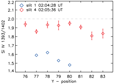
Figure 12: Variations in the Si IV 1393.75 Å and 1402.77 Å line ratio used as a probe for measuring the optical thickness. Blue diamonds indicate the ratios measured in the reconnection region, while red ones away from it and later on.

4.2.3 Diagnostics of the electron density

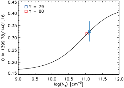
Figure 13: Diagnostics of the electron density using the intensities of the intercombination lines of O IV measured at y = 79 (blue), 80 (red).

The electron density could be computed in the mini flare area, away from the reconnection region (in slit 4) and observed a minute after the reconnection itself. In order to obtain the electron densities we used density-sensitive ratios of line intensities. IRIS routinely observes multiple inter-combination lines which provide ratios useful for this purpose as they are not affected by opacity issues (Polito et al., 2016; Young et al., 2018a). Here, we are able to obtain reliable fits of lines composing only one ratio, being the O IV 1399.78 Å and 1401.16 Å lines. The former line was however still weak, with reliable fits only at slit 4 observed at 02:05:36 UT and for y = 79 and 80.

The measured ratios are presented in Fig. 13. The emissivities are calculated using the dens_plotter.pro routine contained within the CHIANTI package for the peak temperature of formation of the ion (log($T$ [K]) = 5.15). At both locations, the resulting densities are roughly log($N_{\text{e}}$ [cm^-3]) = 11 $\pm$ 0.3. Note that these values correspond to those obtained by Polito et al. (2016) in a plage and a bright point. The mixed ratio proposed by Young et al. (2018a) with Si IV and O IV lines could not be computed due to the low counts.

4.2.4 Path length

Measured electron densities can then be used to calculate $\tau_{\text{0}}$ at the center of the line using e.g. Equation (21) of Dudík et al. (2017):

$$\tau_{\text{0}}\approx 0.26f\frac{\left\langle N_{\text{e}}\right\rangle}{10^{10}\text{ cm}^{-3}},$$ (5)

where $f$ is the path length ($\triangle s$) filling factor in an IRIS pixel defined as $f=\triangle s/0.33\arcsec$. The numerical factor of $0.26$ was by Dudík et al. (2017) calculated using thermal line widths of the resonance lines of Si IV for the Maxwellian distribution. However, the observed profiles of the Si IV lines are much broader. The widths resulting from fits are typically $>$0.5 Å, which reduces the numerical factor down to 0.012. Still, $\tau_{\text{0}}$ cannot be calculated unless the value of $f$ is known. If we for simplicity assume $f=1$ and utilize the measured density of log($N_{\text{e}}$ [cm^-3]) = 11, the modified formula leads to $\tau_{\text{0}}\approx 10^{-1}$. Note that at the same time and positions, ratios of the resonance lines were consistently closer to 2 compared to the values measured in the reconnection region, indicating relatively optically-thinner plasma.

The formula for $\tau_{\text{0}}$ can easily be rewritten in terms of the path length $\triangle s$. Using the relation for $f$ and measurements of the line widths and electron densities, we obtain (in kilometres):

$$\triangle s\approx 2000\tau_{\text{0}}.$$ (6)

Since we relaxed the assumption of $f=1$, the estimate for $\tau_{\text{0}}$ does not hold any further. However, as indicated by the resonance line ratios, outside of the reconnection region it is most likely $<1$ (Section 4.2.2). The possible path lengths are thus determined using the derived linear relation, while their upper boundary is $\approx$2000 km.

As it has been demonstrated for flares in stars (Mathioudakis et al., 1999) if the electron density in the atmosphere is known, opacity can provide important information on the linear dimensions of the scattering layer.

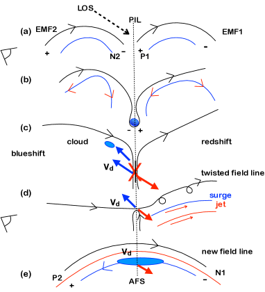
Figure 14: Sketch of the dynamics of the plasma in 2D (x,z) plane at the reconnection site before (panels a and b), during (panels c, d) and after the magnetic reconnection (panel e). The sketch is based on the characteristics of the spectra detailed in table LABEL:table4. Panel (a) corresponds to the time 01:51 UT, panel (b) to 01:59 UT, panel (c) between 02:02:21 and 02:04:28 UT, panel (d) to 02:05:39 UT, and panel (e) to 02:10 UT. The eye on the left side indicates that the observations are done on the side because the AR is located at W 60. The projected line of sight in the plane (x,z) is also shown by dashed arrow at the top. The magnetic field lines are shown with black solid lines with arrows. The vertical central dotted line is the polarity inversion line (PIL) between magnetic polarities N2 and P1. The red solid lines are for hot jet (in panel d) or loops (in panel e) and the velocity directions are indicated by thin blue/red arrows for the transverse flow (panels b and e) and thick arrows for blue/redshifts (V_d) estimated at the PIL zone (panels c, d, e) . In panel (a) EMF1 and EMF2 are two emerging magnetic flux (EMF), and N2-P1 is the bipole where the reconnection occurs in a bald patch with cool material trapped inside (blue circle in panel b). The blue lines and ovals are for the cool plasma visible with IRIS. The reconnection occurs at the ‘X’ point with bidirectional outflows (panel c). The cloud is a blue oval on the left. Nearly at the same time the jet (red line, hot plasma visible in AIA filters) and the surge (blue line) are expelled with some twist to the right (panel d). Panel (e) shows long loops (red line) and an arch filament system (AFS) (blue oval) between P2 and N1 after the reconnection.

5 Discussion and Conclusion

A question arises concerning the height of the magnetic reconnection of the mini flare at the jet base. When jets are observed over the limb like in the paper of Joshi et al. (2020a), the reconnection point is clearly visible in the corona (e.g 10 Mm in the case of Joshi et al. (2020a)). For events occurring on the disk it is difficult to derive the altitude of reconnection. Grubecka et al. (2016); Reid et al. (2017) and Vissers et al. (2019) used a NLTE radiative transfer code in a 1D atmosphere model to derive the altitude of formation of the reconnection in UV burst visible in Mg II lines. The altitude range spans the high photosphere and chromosphere (50 to 900 km). With IRIS it was also found in UV bursts or IRIS bombs (IBs) that cool plasma emitting in chromospheric lines could overlay hotter plasma at Si IV line temperature (Peter et al., 2014). After a long debate about the temperature of the Si IV lines in possibly non equilibrium state, 3D simulation based on Bifrost code (Gudiksen et al., 2011) coupled with the MULTI3D code (Leenaarts & Carlsson, 2009) succeeded to mimic the large observed Si IV profiles (very similar to our UV Si IV burst) and the extended wing of the Ca K line with synthetic profiles both formed at different altitudes simultaneously due to an extended vertical current sheet in a strong magnetized atmosphere (Hansteen et al., 2019). They proposed that “the current sheet is located in a large bubble of emerging magnetic field, carrying with it cool gas from the photosphere”. This scenario is certainly valid for our observations. We attempted to compute the optical thickness and the electron density in the mini flare area during the reconnection process (Kerr et al., 2019; Judge, 2015). The transition lines (Si IV and O IV) usually used for such estimations had so perturbed profiles that no reliable numbers could be put forward at the time of the reconnection. One minute later the Si IV lines were estimated to be nearly optical thin and the computed electron density arises to log($N_{\text{e}}$ [cm^-3]) = 11 $\pm$ 0.3, value which corresponds to a plage or bright point, similarly in the paper of Polito et al. (2016).

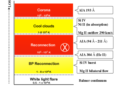
Figure 15: Model of multi-layers of the mini flare atmosphere during the jet reconnection in a bald patch region. The model is based on the observations of emission or absorption of the IRIS lines and continua, and the images of AIA in the multi temperature filters in the mini flare (UV burst) around 02:04:28 UT $\pm$ 60 sec (right column). The y axis is along the LOS. The LOS crosses successively cool and hot layers (white for minimum of temperature, yellow for chromosphere until transition region temperatures, red for coronal temperatures).

However, we have to consider that we have not only the signatures of IBs with IRIS but also the enhancement of Balmer continuum detected in IRIS spectra like in a white light mini flare. The mini flare is also visible as brightenings in all AIA filters with multi temperatures from 10⁵ K to 10⁷ K. This mini flare, called mini flare due to its small area and GOES strength flux (B6.7) is in fact a very energetic flare belonging to the category of white light flares. The chance is that the slit of IRIS with its high spatial and temporal resolution was exactly at the site of the reconnection. Therefore it is the first time that we have such important information on a white light mini flare.

We have all along Sect. 3 discussed on the signatures of the different elements and proposed a dynamical model for the magnetic reconnection in Sect. 4. The analysis of HMI magnetogram of the AR shows that the region consists of several EMFs. The jet occurs between two of them when the negative polarity of the following EMF was collapsing with the positive polarity of the leading EMF. Such magnetic topology leads to a bald patch magnetic configuration where the magnetic field lines are tangent to the photosphere (Paper I). This topology was confirmed by the first reconnection signature in Mg II lines with symmetric extended wings at 02:03:46 UT (Fig. 4 panel (b)) similar to those in IBs commonly occurring in bald patches (Georgoulis et al., 2002; Zhao et al., 2017). At the reconnection site these bilateral outflows ($\pm$ 200 km s^-1) observed in a few pixels were interpreted as reconnection jet (Sect. 3.4). Less than one minute later (02:04:28 UT) extended Mg II line blue wing suggests super Alfvénic flows (Fig. 4 panel (c). With the cloud model technique, which represents a formal solution of the transfer equation under some assumptions, two plasma clouds, one with high speeds (blueshifts of 290 km s^-1) and one with medium speed (blueshifts of 36 km s^-1) were detected (Sect. 3.5). The identification of ”explosive” i.e. 290 km s^-1 flow is unique in such circumstance of reconnection. We conjecture that cool plasma was trapped between the two EMFs which could correspond to arch filament plasma and was expelled during the reconnection. The second cloud with lower velocity is certainly due to the surge plasma accompanying the jet. In the AIA 304 Å movie, dark area was observed at this time looking stationary. The surge plasma could extend along the LOS in a first phase before being elongated along the jet towards the West direction at 02:05:39 UT (Fig. 14 panel (d)).

Table 4: Characteristics of the evolution of the pattern and Mg II spectra of the mini flare at the jet base (reconnection site in X) between the two arch filament systems observed in AIA 304 Å  and in the IRIS slit positions (1-4) (Figs. 2 and 3). The pixel numbers are the coordinates along the slit. This table is discussed in Sect. 3.7 and used to provide a dynamical model of the reconnection in Fig. 14.

Time (UT)	AIA 304 Å	IRIS Mg II spectra
		(slit 1)	(slit 2-3)	(slit 4)
01 :51 :15	Arch Filament Systems (AFS)	redshift at pixel 80	high peaks	blue shift at pixel 80
	over EMF1 and EMF2	strong central absorption	central absorption	central absorption
01 :54 :33	bright threads in X	blue/red shift at pixel 80	broad lines
	between the 2 AFS	central absorption
01 :56 :26	AFS with bright ends	long wings red and blue	large central absorption	thin blue
01 :59 :34	bright threads in X	ten y pixels with broad
	mixed with dark kernels	central absorption
02 :01:10	preflare in X	bright blue along 20 pixels	broad central absorption	thin
02 :02 :21	bright NS arch	extended blue wing profile	blue and broad	thin
02: 02: 59	onset of surge	strong central absorption	shift towards blue
02 :03 :32	kernels	very bright peaks symetrical	blue	blue
02 :04 :28	bright triangle jet base	bright tilt blue to red	large bright blueshift
02 :05 :39	mini flare	very bright blue tilt	bright tilt	bright tilt
	double jet and surge	extended blueshift
02 :06 :22	expansion	zigzag central absorption	zigzag	elongated thin wing
02 :07 :04	long surge over the jet	weak blue peak, redshift	weak broad profiles
02 :10 :21	long loops	thin blue pixel	broad weak	continuum
	bright and dark	weak extended redshift
02 :14 :24	long loops	one pixel extended peaks	weak broad profiles	extended thin blue-red
	long AFS	long red wing extension in y	red
02 :18 :24	end	symmetric profiles	weak broad profiles	continuum

During the reconnection phase at 02:04:28 UT (Fig. 4 panels (b, h, m)) and Fig. 14 (panel c)), we have many signatures of the different elements that allow us to build a multi layer model of the flare atmosphere along the current sheet. We propose for this flare atmosphere the sandwich model with successive cool and hot plasma along the LOS (Fig. 15). Emission at the minimum temperature is also detected with AIA 1600 Å and 1700 Å filters and confirmed this low level heating. Mg II and C II lines are good diagnostics for detecting plasma at chromospheric temperature (T $<$ 20,000K). We identified the bilateral outflows in the bald patches still visible at this time of reconnection in Si IV for example in Fig. 7. The bald patch current sheet is transformed to an ‘X’-point current sheet during the reconnection, which is responsible of the hot plasma detected in the AIA filters (94 Å  to 211 Å), as the MHD model suggests in Paper I. However we have again the signature of cool plasma. In fact Si IV profiles are striped by absorption lines formed at photospheric temperatures and clearly show the presence of cool plasma over transition region temperature material in the reconnection site (Sect. 4.1 and Fig. 8). This cool plasma is certainly due to the cool clouds, either the ejected fast cloud feed by trapped material in bald patch or by surge plasma. All this event is finally embedded in the corona. This demonstrated the possibility of having successive layers in the atmosphere with different velocities and temperatures in the current sheet region.

We have used the cloud model technique as a simple diagnostics tool. Such models are used to derive true velocities which usually differ from those obtained from Doppler shifts (this is the basic idea behind the cloud model). Then the question is what is the nature of the obtained velocities, expelled plasma blobs like in surges (Moreno-Insertis et al., 2008; Nóbrega-Siverio et al., 2018) as we suggested, upflows (evaporation), downflows (chromospheric condensations) as it is proposed for flares (Berlicki et al., 2005; del Zanna et al., 2006). However using the cloud-model technique cannot help us for the proper understanding of the nature of detected flows, it is just a diagnostics method. Numerical simulations using RADYN and RH (Kerr et al., 2019) or Flarix RHD codes (Kašparová et al., 2019) would certainly give more insights on the physical process involved. These observations could be the boundary conditions of future simulations. As we have discussed in section 4.2 we found similarities between such simulation models and our observations like the high variability of the Si IV lines depending strongly on opacity effects.

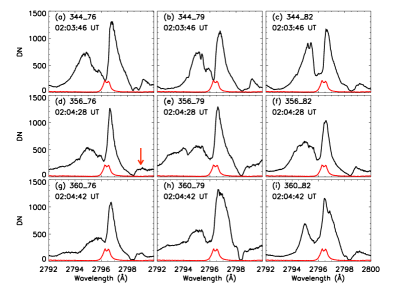
Figure 16: Evolution of Mg II k line profiles inside the UV burst for three times (each row distant of 42 s and 14 s respectively) and for three pixels distant of one arcsec (between each column).The UV burst in located in slit 1. The red profile is the reference profile in the quiet chromosphere. The red arrows indicate the emission of the Mg II triplet lines.

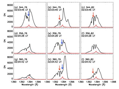
Figure 17: Evolution of Si IV 1393.76 Å line profiles inside the UV burst (same points as in Figure 16) for three times (each row distant of 42 s and 14 s respectively) and for three pixels distant of one arcsec (between each column).The UV burst in located in slit 1. The red profile is the reference profile in the quiet chromosphere. The red arrows indicate the absorption by the Ni II 1393.33 Å  and Fe II 1393.589 Å. The blue arrows indicate the dip in the central Si IV profile due to self absorption.

ANNEX

The spatio-temporal variations of the Mg II k and Si IV profiles are displayed for three times and for three different pixel values in Figures 16 and 17. The profiles vary fast on these time and spatial scales (in 30 sec. and 1$\arcsec$ respectively). We note the need of high spatial and temporal resolution spectra to detect with accuracy the time and the location of reconnection.