Prediction-Based Power Oversubscription in Cloud Platforms

Abstract

Datacenter designers rely on conservative estimates of IT equipment power draw to provision resources. This leaves resources underutilized and requires more datacenters to be built. Prior work has used power capping to shave the rare power peaks and add more servers to the datacenter, thereby oversubscribing its resources and lowering capital costs. This works well when the workloads and their server placements are known. Unfortunately, these factors are unknown in public clouds, forcing providers to limit the oversubscription so that performance is never impacted.

In this paper, we argue that providers can use predictions of workload performance criticality and virtual machine (VM) resource utilization to increase oversubscription. This poses many challenges, such as identifying the performance-critical workloads from black-box VMs, creating support for criticality-aware power management, and increasing oversubscription while limiting the impact of capping. We address these challenges for the hardware and software infrastructures of Microsoft Azure. The results show that we enable a $2\times$ increase in oversubscription with minimum impact to critical workloads.

I Introduction

Motivation. Large Internet companies continue building datacenters to meet the increasing demand for their services. Each datacenter costs hundreds of millions of dollars to build. Power plays a key role in datacenter design, build out, IT capacity deployment, and physical infrastructure cost.

The power delivery infrastructure forms a hierarchy of devices that supply power to different subsets of the deployed IT capacity at the bottom level. Each device includes a circuit breaker to prevent damage to the IT infrastructure in the event of a power overdraw. When a breaker trips, the hardware downstream loses power, causing a partial blackout.

To avoid tripping breakers, designers conservatively provision power for each server based on either its maximum nameplate power or its peak draw while running a power-hungry benchmark, such as SPEC Power [19]. The maximum number of servers is then the available power (or breaker limit) divided by the per-server provisioned value. This provisioning leads to massive power under-utilization. As the IT demand increases, it also requires building new datacenters even when there are available resources (space, cooling, networking) in existing ones, thus incurring huge unnecessary capital costs.

To improve efficiency and avoid these costs, prior work has proposed combining power capping and oversubscription [9, 32]. The idea is to leverage actual server utilization and statistical multiplexing across workloads to oversubscribe the delivery infrastructure by adding more servers to the datacenter, while ensuring that the power draw remains below the breakers’ limits. This is achieved by continuously monitoring the power draw at each level and using power capping (via CPU voltage/frequency and memory bandwidth throttling), when necessary. As throttling impacts performance, these approaches carefully define which workloads can be throttled and by how much. For example, Facebook’s Dynamo relies on predefined workload priority groups, and throttles each server based on the priority of the workload it runs [32]. Using Dynamo, Facebook was able to oversubscribe its datacenters by 8%, lowering costs by hundreds of millions of dollars.

This oversubscription approach works well when workloads and their server placements are known. Unfortunately, public cloud platforms violate these assumptions. First, each server runs many VMs, each with its workload, performance, and power characteristics. Hence, throttling the entire server would impact performance-critical (e.g., interactive services) and non-critical (e.g., batch) workloads alike. Second, VMs dynamically arrive and depart from each server, producing varying mixes of characteristics and preventing predefined server groupings or priorities. Third, each VM must be treated as a black box, as customers are often reluctant to accept deep inspection of their VMs. Thus, the platform does not know which VMs are performance-critical and which ones are not. For these reasons, oversubscription in public clouds has been limited so that performance is never impacted.

Our work. In this paper, we argue that cloud providers can increase oversubscription substantially by carefully scheduling VMs and managing power, based on predictions of workload performance criticality and VM CPU utilization. Our insight is that there are many non-critical workloads (e.g., batch jobs) that can tolerate a slightly higher rate of capping events and/or deeper throttling; the capping of performance-critical workloads must be controlled more tightly. Using predictions to identify these workloads and place them carefully across the datacenter provides the power slack and criticality-awareness needed to increase oversubscription.

Accurately predicting (black-box) workload criticality is itself a challenge. Prior work [6] associated a diurnal utilization pattern with user interactivity and the critical need for high performance. It inferred criticality using the Fast Fourier Transform (FFT) algorithm on the CPU utilization time series for each workload. Here, we present a more accurate and robust pattern-matching algorithm, and a machine learning (ML) model that uses the algorithm’s output during training. We also propose a model for predicting the 95th-percentile CPU utilization over a VM’s lifetime.

With these predictions, we increase the power slack in the datacenter by balancing the expected power draw and our ability to lower it via throttling when a power budget is exceeded (causing a capping event). We accomplish this with a criticality- and utilization-aware VM placement policy. When events occur, we must cap power intelligently as well. So, we propose a system that protects performance-critical VMs from throttling when capping a server’s power draw.

Using the above contributions and the history of power draws, we devise a new strategy for selecting the amount of oversubscription. The strategy limits the impact of capping on the two VM types to predefined acceptable values, thereby enabling significant but controlled increases in oversubscription. Providers that prefer to treat all external (i.e., third-party) VMs the same can simply assume them all to be critical, and classify only the internal (i.e., first-party) VMs into the two types at the cost of a lower increase in oversubscription.

We implement our work for the hardware, firmware, and software of Microsoft Azure. Specifically, we implement our criticality algorithm and ML models for Azure’s ML and prediction-serving system; implement our VM placement policy as an extension of Azure’s VM scheduler; implement our per-VM capping system as a host-level agent on each server, and leverage Azure’s capping mechanisms; and implement our oversubscription strategy using Azure’s historical power and utilization telemetry.

The evaluation shows that our criticality algorithm is substantially more accurate than FFTs, and that our ML models achieve high prediction accuracy. Our system and policy have not yet been deployed widely, so we evaluate them on the same hardware, firmware, and software that runs in production, but in an isolated environment. We also show that our system and policy lower the performance impact of a capping event, while our policy produces fewer events. Overall, we can increase oversubscription by $2\times$ (from 6 to 12%), compared to the state-of-the-art approach. This increase would save $75.5M in capital costs from just one datacenter site (128MW). Assuming that all external VMs are performance-critical would lower the savings to a still significant $28.1M. Large cloud providers have many such sites, so these savings would multiply.

We have started deploying our work in production at Microsoft and mention some lessons in Section V.

Related work. The prior work on power capping [13, 15, 20, 22, 23, 24, 25, 27, 34] and oversubscription [9, 11, 14, 21, 29, 31, 32] produced major advances in server and datacenter power management. Unfortunately, it falls short for real public clouds. For example, it has capped server power using inputs that are typically not available in the public cloud, such as application-level metrics or operator annotations. Moreover, it has employed reactive and expensive VM migration in clusters, instead of leveraging predictions for capping and capping-aware scheduling. Prior oversubscription works have focused on non-cloud datacenters and full-server capping when workloads and their priorities are known.

Summary. We make the following main contributions:

1. An algorithm and ML model for predicting performance criticality, and a model for predicting VM utilization.

2. A VM placement policy that uses these predictions to minimize the number of capping events and their impact.

3. A per-VM power capping system that uses predictions of criticality to protect certain VMs.

4. A strategy that leverages the contributions above to increase the amount of oversubscription.

5. Implementation and results for the infrastructure of Azure, showing large potential cost savings.

6. Lessons from production deployment of our work.

Though we build upon Azure’s infrastructure, our conceptual contributions (e.g., predicting criticality; using predictions in VM placement, power budget enforcement, and oversubscription) apply directly to any cloud platform.

II Background and Context

II-A Typical power delivery and server deployment

At the top of the power delivery hierarchy, the electrical grid provides power to a sub-station that is backed up by a generator. An Uninterruptible Power Supply (UPS) unit provides battery backup while the generator is starting up. The UPS feeds one power distribution unit (PDU) per row of servers. Each row PDU supplies power to several rack PDUs, each of which feeds a few server chassis. Each chassis contains a few power supplies (PSUs) and dozens of blade servers. A PDU trips its circuit breaker when the power draw exceeds the rated value (budget) for the unit, causing a power outage.

Designers deploy servers so that breakers never trip, leading to wasted resources (chiefly space, cooling, and networking). Combining hierarchical power capping and oversubscription enables more capacity to be deployed and better utilizes resources [9, 32]. For example, if designers find that the historical per-row power draw is consistently lower than the row PDU budget, they can “borrow” power from each row to add more rows (until they run out of row space) under the UPS budget. The extra rows oversubscribe the power at the UPS level. The servers downstream from the oversubscribed PDUs/UPS must be power-capped, whenever they are about to draw power that has already been borrowed.

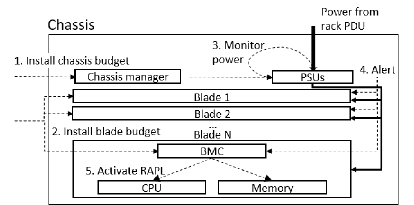
Figure 1: Chassis-level alert-based power capping.

II-B Azure’s existing power capping mechanisms

For clarity and ease of experimentation, in this paper we explore power budget enforcement at the chassis level.

Figure 1 shows Azure’s current mechanisms. Each chassis contains a manager that exposes the management interface. To enable capping, Azure first sets the total chassis-level power budget at the chassis manager and PSUs (step 1), and each individual blade power cap in its board management chip (BMC) (step 2). Azure sets each blade budget to its even share of the chassis budget.

Under normal operation, no capping takes place, i.e. each server is free to draw more power than its even share, as long as the total chassis draw is below the chassis budget. The PSUs monitor the chassis draw (step 3) and alert the blades directly when the chassis budget is about to be exceeded (step 4). Upon an alert, the blade power must be brought below its even-share cap. (Uneven caps are infeasible due to the overhead of dynamically reapportioning and reinstalling blade budgets.) The BMC splits the cap evenly across its sockets and uses Intel’s Running Average Power Limit (RAPL) [7] to lower the blade power (step 5). RAPL throttles the entire socket (slowing down all cores equally) and memory using a feedback loop until the cap is respected. Typically, RAPL brings the power below the cap in less than 2 seconds.

II-C Azure’s existing VM scheduler

A cloud platform first routes an arriving VM to a server cluster. Within each cluster, a VM scheduler is responsible for placing the VM on a server. The scheduler uses heuristics to tightly pack VMs, considering the incoming VM’s multiple resource requirements and each server’s available resources.

Azure’s scheduler implements its heuristics as two sets of rules. It first applies constraint rules (e.g., does the server have enough resources for the VM?) to filter invalid servers, and then applies preference rules each of which orders the candidate servers based on a preferred metric (e.g., a packing score derived from available resources). It then weights each candidate based on its order on the preference list for each rule and the rule’s pre-defined weight. Finally, it picks a server with the highest aggregate weight for allocation. No rules currently consider power draws or capping.

II-D Azure’s existing ML system

To integrate predictions into VM scheduling in practice, we target Resource Central [6], the existing ML and prediction-serving system in Azure. The system provides a REST service for clients (in our case the VM scheduler) to query for predictions. It can receive input features (e.g., user, VM size, guest OS) that are known at deployment time from the scheduler, execute one of our ML models (criticality or CPU utilization), and respond with the prediction and a confidence score. Model training is done in the background, e.g. once a day.

III Prediction-Based Oversubscription

Cloud providers provision servers conservatively, and have full-server capping mechanisms and capping-oblivious VM schedulers. We propose to provision servers more aggressively by making the infrastructure smarter and finer-grained via VM behavior predictions. Key challenges include having to create or adapt many components (e.g., scheduler, chassis manager) to the predictions, while ensuring that the tradeoff between oversubscription and performance is tightly controlled.

Next, we overview our design and then detail its main components. Then, we describe our strategy for provisioning servers to balance cost savings and performance impact.

III-A Overview

Figure 2 overviews our system and its operation, showing the existing and new/modified components in different colors. We modify the VM scheduler to use predictions of VM performance criticality and resource utilization. We implement our ML models so they can be managed and served by the existing ML and prediction-serving system. We modify the chassis manager to query the chassis power draw and interact with our new per-VM power controller. The controller manages its server’s power draw during a capping event.

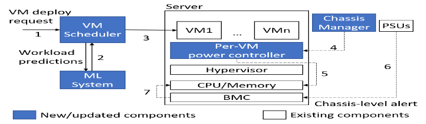
Figure 2: System overview.

In detail, a request to deploy a set of VMs arrives at our VM scheduler (arrow #1). The scheduler then queries the ML system for predictions of workload performance criticality and resource utilization (#2). Using these predictions, it decides on which servers to place the VMs (#3). After selecting each VM’s placement, the scheduler tags the VM with its predicted workload type and instructs the destination server to create it. Each chassis manager frequently polls its local PSUs to determine whether the power draw for the chassis crosses a threshold just below the chassis budget. (This threshold enables the controller to perform per-VM capping and hopefully avoid needing full-server RAPL.) When this is the case, the manager alerts the controller of each server in the chassis (#4).

Upon receiving the alert, the controller at each server manages the server’s (even) share of the chassis budget across the local VMs based on their workload types. It does this by first throttling the CPU cores used by non-performance-critical VMs (#5). Throttling these VMs may be enough to keep the power below the chassis budget, and protect the performance-critical VMs. If it is not enough, the PSUs alert the servers’ BMCs (#6), which will then use RAPL as a last resort to lower the chassis power below the budget (#7).

Limiting impact on non-critical VMs. Though we protect critical VMs from throttling, we limit the performance impact on non-critical VMs in three ways. First, for long-term server provisioning, our oversubscription strategy carefully selects chassis budgets to limit the number of capping events and their severity to predefined acceptable values (e.g., no more than 1% events for non-critical VMs, each lowering the core frequency to no less than 75% of the maximum). Second, for medium-term management, our scheduler places VMs seeking to minimize the number of events and their severity. Finally, in the shortest term, our per-VM controller increases the core frequency of non-critical VMs as soon as possible.

Treating external VMs as performance-critical. Providers who prefer to treat all paying customers the same can easily do so by assuming that all external VMs are performance-critical; only internal VMs (e.g., running the provider’s own managed services) would be classified into the two criticality types. We explore this assumption in Section IV-F.

III-B Predicting VM criticality and utilization

Our approach depends on predicting VM performance criticality and utilization at arrival time, i.e. just before the VMs are deployed. We train supervised ML models to produce these predictions based on historical VM arrival data and telemetry that was collected after those VMs were deployed. Since VMs are black boxes, our telemetry consists of CPU utilization data only, as deep inspection is not an option.

Inferring criticality. Predicting criticality requires a method to determine the VM labels, i.e. whether the workload of each VM is performance-critical or not, before we can train a model. As in prior work [6], we consider a workload critical if it is user-facing, i.e. a human is interacting with the workload (e.g., front-end webservers, backend databases), and less critical otherwise (e.g., batch, development and testing workloads). As user-facing workloads exhibit utilization patterns that repeat daily (e.g., high during the day, low at night), the problem reduces to identifying VMs whose time series of CPU utilizations exhibit 24-hour periods [6].

Obviously, some background VMs may exhibit 24-hour periods. This is not a problem as we seek to be conservative (i.e., it is fine to classify a non-user-facing workload as user-facing, but not vice-versa). Moreover, some daily batch jobs have strict deadlines, so classifying them as user-facing correctly reflects their needs. Importantly, focusing on the CPU utilization signal works well even when the CPU is not the dominant resource, as the CPU is always a good proxy for periodicity (e.g., network-bound interactive workloads exhibit more CPU activity during the day than at night).

We considered but discarded other approaches for inferring whether a VM’s workload is user-facing. For example, observing whether a VM exchanges messages does not work because many non-user-facing workloads communicate externally (e.g., to bring data in for batch processing).

Identifying periodicity. There are statistical methods for identifying periods in time series, such as FFT or the auto-correlation function (ACF). For example, [6] assumes a workload is user-facing if the FFT indicates a 24-hour period. We evaluated ACF and FFT methods on 840 workloads on Azure. Surprisingly, we find that both methods lead to frequent mis-classifications. We identify three culprits:

1. The diurnal patterns in user-facing workloads often have significant noise and interruptions. For example, we observe user-facing workloads with clear 24-hour periods for many days, interrupted by a period of constant or random load, causing them to be mis-classified as non-user-facing.

2. The diurnal patterns often exhibit increasing/decreasing trends (e.g., the workload becomes more popular over time), and varying magnitudes of peaks/valleys across days. These effects cause some user-facing workloads to be mis-classified.

3. There are many machine-generated workloads with periods of 1 hour, 4 hours, 6 hours or other divisors of 24 hours, which therefore also have 24-hour periods, leading to machine-generated workloads that are mis-classified as user-facing.

Part of the problem is that ACF and FFT are very general tools with different goals, e.g. decomposing a signal for compact representation and capturing general correlations, not solutions for our specific problem of 24-hour periods.

Criticality algorithm. Thus, we devise a new algorithm that is more robust and targeted at our specific problem. Our idea is to extract from a VM’s utilization time series a template for a typical 24-hour period and then check how well this template captures most days in the series. We design the template extraction and comparison to be robust to noise and interruptions to deal with issue #1 above. We pre-process the data using methods from time series analysis to address #2. To deal with #3, we extract templates for shorter periods (8 and 12 hours) and ensure that the 24-hour template is the best fit. These periods subsume the other short periods.

More precisely, the input to our pattern-matching algorithm is the average CPU utilization for each 30-minute interval over 5 weekdays. (Shorter workloads cannot be classified and should be conservatively assumed user-facing.) For each utilization time series, the algorithm does the following:

1. It de-trends and normalizes the time series, so that all days exhibit utilizations within the same rough range. De-trending scales each utilization based on the mean of the previous 24 hours, whereas normalization divides each utilization by the standard deviation of the whole time series.

2. It extracts the 24-hour template by identifying, for each time of the day (in 30-minute chunks), its “typical” utilization computed as the median of all utilizations in the pre-processed series that were reported at this time of the day.

3. It overlays the template over the pre-processed series for each day and computes the average deviation for each utilization, after excluding the 20% largest deviations.

4. It repeats steps 2 and 3 to compute average deviations for 8-hour and 12-hour templates, and then computes two scores: 24-hour average deviation divided by 8-hour average deviation (called Compare8), and 24-hour average deviation divided by 12-hour average deviation (called Compare12). If the scores are close to 0, the workload is likely to be user-facing. Ultimately, it classifies a time series as user-facing, if its Compare8 value is lower than a threshold (Section IV-B).

Criticality prediction. The algorithm above produces labels that we use to train an ML model to classify arriving VMs as user-facing or non-user-facing. Specifically, we train a Random Forest using the labels and many features (pertaining to the arriving VM and its cloud subscription) available at arrival time: the percentage of user-facing VMs in the subscription, the percentage of VMs that lived at least 7 days in the subscription, the total number of VMs in the subscription, the percentage of VMs in each CPU utilization bucket, the averages of the VMs’ average and 95th-percentile CPU utilizations in the subscription, the arriving VM’s number of cores and memory size, and the arriving VM’s type.

Utilization prediction. For utilization predictions, we train a two-stage model to predict 95th-percentile VM CPU utilization based on labels produced by previous VM executions (actual 95th-percentile utilizations over the VMs’ lifetimes) and the same VM features we use in the criticality model. Since predicting utilization exactly is hard, our model predicts it into 4 buckets: 0%-25%, 26%-50%, and so on. The first stage of the model is a Random Forest that predicts whether or not the 95th-percentile utilization is above 50%. In the second stage, we have a Random Forest for buckets 1-2 and another for buckets 3-4. We train these latter forests with just the VMs we can predict with high-confidence ($\geq$ 60%) in the first stage.

We experimented with single-stage models, but they did not produce accurate predictions with enough confidence.

III-C Modified VM scheduler

Our ability to increase oversubscription and the efficacy of the per-VM power controller depend on the placement of VMs in each cluster. Better placements have a balanced distribution of power draws across the different chassis to reduce the number of capping events (Goal #1); and a balanced distribution of cap-able power (drawn by non-user-facing VM cores) across servers, so the controller can lower the power during an event without affecting critical VMs (Goal #2). The scheduler must remain effective at packing VMs while minimizing the number of deployment failures (Goal #3).

Given these goals, we modify Azure’s VM scheduler to become criticality- and utilization-aware, using predictions at VM arrival time. Our policy is a preference rule that sorts the feasible servers based on a “score”. Each server’s score considers the predicted 95th-percentile CPU utilization of the VMs already placed in the same chassis (targets Goal #1), and the predicted criticality and 95th-percentile CPU utilization of the VMs already placed on the same server (targets Goal #2). The policy only considers CPU utilization because the CPUs are the dominant source of dynamic power in Azure’s servers. As Section IV-E shows, our policy does not degrade the packing of VMs onto servers, nor does it increase the percentage of VM deployment failures (achieves Goal #3).

1:function SortCandidates($V$, $\zeta$) $\triangleright$ $V$: VM to be placed, $\zeta$: list of candidate servers

2:    $\omega\leftarrow V^{PredictedWorkloadType}$

3:    for $c_{i}$ in $\zeta$ do

4:        $\kappa_{i}\leftarrow\textsc{ScoreChassis}(c_{i}.Chassis)$

5:        $\eta_{i}\leftarrow\textsc{ScoreServer}(\omega,c_{i})$

6:        $c_{i}.score\leftarrow\alpha\times\kappa_{i}+(1-\alpha)\times\eta_{i}$     

7:    return $\zeta.\textsc{sortDesc}(c_{i}.score)$

8:function ScoreChassis($C$)

9:    for $n_{i}$ in $C.Servers$ do

10:        for $v_{j}$ in $n_{i}^{VMs}$ do

11:           $\rho^{Peak}\leftarrow\rho^{Peak}+v_{j}^{PredictedP95Util}\times v_{j}^{cores}$         

12:        $\rho^{Max}\leftarrow\rho^{Max}+n_{i}^{cores}$     

13:    return $1-\left[\frac{\rho^{Peak}}{\rho^{Max}}\right]$

14:function ScoreServer($\omega$, $N$)

15:    for $v_{i}$ in $N^{UF\_VMs}$ do

16:        $\gamma^{UF}\leftarrow\gamma^{UF}+v_{i}^{PredictedP95Util}\times v_{i}^{cores}$     

17:    for $v_{i}$ in $N^{NUF\_VMs}$ do

18:        $\gamma^{NUF}\leftarrow\gamma^{NUF}+v_{i}^{PredictedP95Util}\times v_{i}^{cores}$     

19:    if $\omega=UF$ then

20:        return $\frac{1}{2}\times\left(1+\frac{\gamma^{NUF}-\gamma^{UF}}{N^{cores}}\right)$

21:    else

22:        return $\frac{1}{2}\times\left(1+\frac{\gamma^{UF}-\gamma^{NUF}}{N^{cores}}\right)$     

Algorithm 1 Criticality- & utilization-aware VM placement

Algorithm 1 shows our rule ($SortCandidates$) and two supporting routines. We show the predictions with the PredictedWorkloadType and PredictedP95Util superscripts. The rule ultimately computes the score for each candidate server (line #6). The higher the score, the more preferable the server. The score is a function of how preferable the server (line #5) and its chassis (line #4) are for the VM to be placed. Both server and chassis intermediate scores range from 0 to 1. We weight the intermediate scores to give them differentiated importance. We select the best value for the $\alpha$ weight in Section IV-E.

Function $ScoreChassis$ computes the chassis score for a candidate server by conservatively estimating its aggregate chassis CPU utilization, i.e. assuming all VMs scheduled to the chassis are at their individual 95th-percentile utilization at the same time. This value is the sum of the predicted 95th-percentile utilizations for the VMs scheduled to the chassis, divided by the maximum core utilization (#cores in chassis$\times$100%). This ratio is proportional to utilization. We subtract it from 1, so that higher values are better (line #13).

Function $ScoreServer$ scores a candidate server differently depending on the type of VM that is being deployed. First, it sums up the predicted 95th-percentile utilizations of the user-facing VMs (lines #15-16) and non-user-facing VMs (lines #17-18) independently. When a user-facing VM is being deployed, we compute how much more utilized the non-user-facing VMs on the server are than the user-facing ones. We do the reverse for a non-user-facing VM. The reversal is the key to balancing the cap-able power across servers. Adding 1 and dividing by 2 ensure that the resulting score will be between 0 and 1 (lines #20 and #22), while higher values are better.

The algorithm takes only 7 milliseconds, which is negligible as VM creation takes on the order of seconds [1].

III-D Per-VM power capping controller

Azure’s existing in-server capping system uses RAPL and out-of-band (i.e., independently of software on the server) PSU alerts to throttle all cores equally. This approach is simple and safe, but may strongly impact the user-facing workloads. On the other hand, a software-only approach that runs in-band (i.e., as a platform-level service) can be aware of workload types, poll the PSUs, and use per-core DVFS to cap non-user-facing VMs when necessary. However, this solution is vulnerable to software defects and communication issues.

To achieve safety and flexibility, we use a hybrid solution. Our modified chassis manager polls the PSUs every 200 milliseconds and alerts our in-band controller when the chassis power draw is close to the chassis budget. The controller uses per-core DVFS to cap the cores running non-user-facing VMs. To account for (1) high power draws that may occur between polls or (2) the inability of the controller to bring power below the budget, we use the out-of-band mechanisms as a backup.

To power-manage the cores per-VM, we use the core-grouping feature of the hypervisor (e.g., cpupools in Xen, cpugroups in Hyper-V) to split the logical cores into two classes: high-priority and low-priority. We assign the user-facing VMs and the I/O VM (e.g., Domain0 in Xen, Root VM in Hyper-V) to the high-priority class, and the non-user-facing VMs to the low-priority one. The hypervisor ensures that any threads associated with the given VM are scheduled only on the logical cores of its group.

Upon receiving an alert from the chassis manager, the per-VM power controller compares the server’s power draw to its budget. If the current draw is higher than the budget, the controller immediately lowers the frequency of the low-priority cores to the minimum p-state, i.e. half of the maximum frequency; the lowering of the frequency may entail a lower voltage as well. The goal is to lower the server’s power draw as quickly as possible without affecting the important workloads. However, this large frequency reduction may overshoot the needed power reduction. To reduce the impact on the non-user-facing VMs, the controller then enters a feedback loop where each iteration involves (1) checking the server power meter and (2) increasing the frequency of $N$ low-priority cores to the next higher p-state, until the power is close to the budget. It selects the highest frequency that keeps the power below this threshold. $N$ = 4 works well in our experiments.

It is possible that cutting the frequency of the low-priority cores in half is not enough to bring the power below the server’s budget. For example, a VM placement where there are not enough non-user-facing VMs in the workload mix, non-user-facing VMs exhibiting lower utilization than predicted, or a controller bug can cause this problem. In this case, the out-of-band mechanism will kick in as backup. Though RAPL will apply to all cores indiscriminately, protection from overdraw must take precedence over performance loss.

The controller lifts the cap after some time (30 secs by default), allowing all cores to return to maximum performance.

III-E Oversubscription strategy

We now describe our oversubscription strategy, which uses our capping system and placement policy, historical VM arrivals, and historical power draws, to increase server density. It relies on the algorithm below for computing an aggressive power budget for all the chassis of each hardware generation. Adapting it to find budgets for larger aggregations (e.g., rack, row) is straightforward. We refer to the uncapped, nominal core frequency as the “maximum” frequency.

To configure the algorithm, we need to select the maximum acceptable rate of capping events (e.g., #events per week) for user-facing ($emax_{UF}$) and non-user-facing ($emax_{NUF}$) VMs, and the minimum acceptable core frequency (e.g., half the maximum frequency) for user-facing ($fmin_{UF}$) and non-user-facing ($fmin_{NUF}$) VMs. If we want no performance impact for user-facing VMs, we set $emax_{UF}=0$ and $fmin_{UF}=$ maximum frequency. As we describe next, our 5-step algorithm finds the lowest chassis power budget that satisfies $emax_{UF},emax_{NUF},fmin_{UF},$ and $fmin_{NUF}$.

Estimate future behaviors based on history:

1. Estimate the historical average ratio of user-facing virtual cores in the allocated cores ($\beta$). Estimate the historical average P95 utilization of virtual cores in user-facing ($util_{UF}$) and non-user-facing ($util_{NUF}$) VMs.

Profile the hardware:

1. Estimate how much server power can be reduced by lowering core frequency at $util_{UF}$ and $util_{NUF}$, given $fmin_{UF}$ and $fmin_{NUF}$, respectively. This step produces two curves for power draw (one curve for each average utilization), as a function of frequency.

Compute power budgets based on historical draws:

1. Sort the historical chassis-level power draws (one reading per chassis per unit of time) in descending order.

2. Start from the highest power draw as the first candidate budget and progressively consider lower draws until we find $P_{min}$. For each candidate power budget, we check that the rate of capping events would not exceed $fmax_{UF}$ or $fmax_{NUF}$ (considering the higher draws already checked), and the attainable power reduction from capping is sufficient (given $\beta$ and the curves from step 2).

3. To compute the final budget, add a buffer (e.g., 10%) to the budget from step 4 to account for future variability of $\beta$ or substantial increases in chassis utilization.

We can use the difference between the overall budget computed in step 5 and the provisioned power to add more servers to the datacenter. Because we protect user-facing VMs and use our VM scheduling policy, this difference is substantially larger than in prior approaches, as we show in Section IV-F.

Example. Suppose we are willing to accept rates of 0.1% and 1% capping events for user-facing and non-user-facing VMs, respectively. Suppose further that, upon a capping event, we are willing to lower the core frequencies to 75% and 50% of the maximum, respectively. Now, assume we have 10000 historical chassis power draws (collected from every chassis), and that the highest draws have been 2900W, 2850W, and 2850W. We first consider 2900W. If we were to set the chassis budget to just below that value to say 2890W, there would be 1 capping event out of 10000 observations, i.e. a rate of 0.01%, and we would have to shave 10W during the event. Given the acceptable capping rates and minimum frequencies, we can operate with the data from step 1 and the curves from step 2 to determine (1) whether we could reduce power by 10W, and (2) whether there would be an impact on user-facing VMs. If we can achieve the reduction, we count 1 event out of 10000 that would affect non-user-facing VMs. If the user-facing VMs would also have to be throttled, we would count 1 event out of 10000 that would affect those VMs. Since both rates are lower than 0.1% and 1%, we can now check a budget just below 2850W, say 2840W. We repeat the process for this budget, which would lead to 3 events out of 10000, and the need to lower power by 60W (2900-2840) once and 10W (2850-2840) twice. Then the next lower draw and so on, until we violate the desired capping rates and minimum frequencies.

IV Evaluation

IV-A Methodology

Data analysis. We evaluate our criticality algorithm and ML models (Section IV-B) using standard metrics, such as precision and recall from predictions. We compute the metrics based on the entire VM workload of Azure in April 2019.

Real experiments. We run experiments on the same hardware that Azure uses in production. We use a chassis with 12 servers, each containing 40 cores split into two sockets. At their nominal frequency, each server draws between 112W (idle) and 310W (100% CPU utilization). At half this frequency, each server draws from 111W to 169W.

Our single-server experiments (Section IV-C) explore the dynamic behavior of our per-VM power capping controller and resulting VM workload performance for a combination of user-facing and non-user-facing VMs and various power budgets. For comparison, we use the existing full-server capping controller (Intel’s RAPL) in Azure. Our chassis-level experiments (Section IV-D) explore our system on 12 servers, including PSU alerts. For comparison, we use the existing chassis-level mechanisms in Azure (Figure 1).

For both sets of experiments, we use instances of a latency-critical transaction processing application (similar to TPC-E) for the user-facing workload, and instances of a batch Hadoop computation (Terasort) for the non-user-facing workload. For the user-facing workload, we use real inputs from Azure’s team responsible for it, whereas we use synthetic input data for the non-user-facing computation.

Simulation. We evaluate our modified VM scheduler in simulation (Section IV-E), leveraging the same simulator that Azure uses to evaluate changes to the VM scheduler before putting them in production; our only extension is to simulate calls to the ML system. An event generator drives the simulation with a sequence of VM arrivals. For each arrival, it invokes the production scheduling algorithm (or the scheduling algorithm with the addition of our policy) for server placement decisions. Running the actual scheduler code in the simulator ensures that simulations are faithful to reality.

We simulate a cluster of 60 chassis in 20 racks. The simulator produces VM arrivals based on distributions matching Azure’s load in April 2019. Table I lists the main statistics.

Parameter	Value
Cluster configuration	20 racks $\times$ 3 chassis $\times$ 12 blades
Blade configuration	2x20 cores
VM size dist. (cores)	1 (33%), 2 (27%), 4 (21%), 8 (10%), 16 (5%), 24 (3%), $>=$32 (1%)
Deployment size dist. (#VMs)	1 (39%), 2 (14%), 3-5 (16%), 6-10 (9%), 11-15 (8%), 16-25 (5%), $>$25(9%)
VM lifetime dist. (hours)	1 (52%), 2 (5%), 3-5 (10%), 6-10 (9%), 10-25(7%), 26-720 (8%), $>$720 (9%)
Workload type buckets	user-facing (UF), non-user-facing (NUF)
P95 utilization buckets	0-25%, 26-50%, 51-75%, 76-100%
Avg UF:NUF core ratio	4:6
Avg UF and NUF P95 util	65% (bucket #3), 44% (bucket #2)
# simulation days	30

TABLE I: Simulation parameters.

Technique	Recall	Recall	Precision
	target	achieved	achieved
Pattern-matching	99%	99%	76%
ACF	99%	99%	54%
FFT	99%	99%	48%
Pattern-matching	98%	98%	77%
ACF	98%	98%	56%
FFT	98%	98%	50%

TABLE II: Pattern-matching vs ACF vs FFT.

Prediction	Model	% High	Bucket 1	Bucket 2	Bucket 3	Bucket 4	Accuracy
		Conf.	R — P	R — P	R — P	R — P
Criticality	GB	99%	67% — 77%	99% — 99%	NA	NA	98%
	RF	99%	69% — 78%	99% — 99%	NA	NA	98%
P95 util	GB	68%	95% — 85%	47% — 77%	51% — 79%	94% — 80%	82%
	RF	73%	93% — 87%	61% — 76%	65% — 81%	92% — 83%	84%

TABLE III: Random Forest (RF) and Gradient Boosting (GB) models recall (R), precision (P), and accuracy for high-confidence predictions.

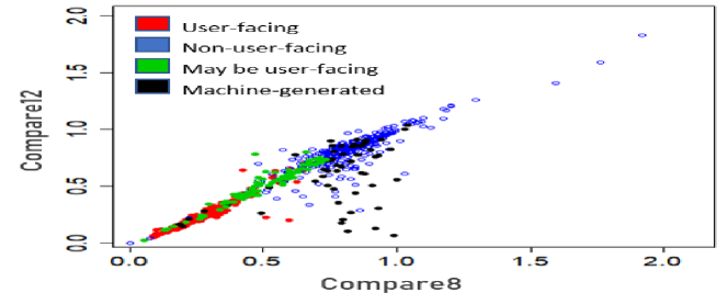
Figure 3: Algorithm compared to manual classification.

IV-B Criticality algorithm and ML models

Criticality algorithm. To evaluate our pattern-matching algorithm (Section III-B), we first compare its classifications to our own manual labeling of 840 workloads on Azure. Figure 3 shows one colored dot for each workload with coordinates corresponding to its Compare8 and Compare12 values. The colors indicate whether we deem the workload clearly user-facing, possibly user-facing, clearly machine-generated, or clearly non-user-facing. The figure shows that Compare8 can separate the first two groups, which the algorithm should conservatively classify as user-facing, from the last two. A vertical bar at Compare8=0.72 gets all important workloads to the left of the bar, and the vast majority of unimportant ones to the right of it. Compare12 does not separate the classes well.

Thus, the algorithm can accurately classify workloads based on their Compare8 value. For a quantitative assessment, we compare it to two well-known approaches for finding periodicity in a time series, ACFs and FFTs, for the same set of workloads. For both approaches, we do the same pre-processing and disambiguate between user-facing and machine-generated workloads using the same methods as in our algorithm.

As we want to protect user-facing VMs, we must achieve high recall for this class as the recall indicates the probability of correctly identifying these VMs. Table III shows the precision and recall, for two high recall targets (0.99 and 0.98) for whether a workload is user-facing. Our algorithm achieves the target recall with much higher precision than its counterparts.

ML models. We now evaluate our models for Azure’s entire VM workload. Table III lists the percentage of predictions with confidence score higher than 60% (3rd column), and the per-bucket recalls and precisions (4th-7th columns) and the accuracy (rightmost column) for those high-confidence predictions. The VM scheduler disregards predictions with lower confidence and conservatively assumes the VM being deployed will be user-facing and will exhibit 100% 95th-percentile utilization. For comparison, we show results for the equivalent Gradient Boosting (GB) models.

The table shows that our criticality model achieves 99% recall for user-facing VMs (Bucket 2), which is critical for protecting these VMs. The most important features for our model are the percentage of user-facing VMs observed in the cloud subscription, the percentage of VMs that live longer than 7 days in the subscription, and the total number of VMs in the subscription. The GB model achieves similar results.

Our utilization model also does well with good recall and precision (83-93%) for the most popular buckets (1 and 4), and good accuracy (84%) for the 73% of high-confidence predictions. Here, the most important features are the average of the VMs’ 95-percentile CPU utilizations in the subscription, the average of the VMs’ average CPU utilizations in the subscription, and the percentages of VMs in each CPU utilization bucket in the subscription. The GB model achieves similar accuracy, but with fewer high-confidence predictions and lower recall for the two middle (least popular) buckets.

IV-C Per-VM capping controller experiments

We run experiments on a server with our user-facing application running on a VM with 20 virtual cores and our non-user-facing application running simultaneously on another VM with 20 virtual cores. Each execution takes 10 minutes.

Figure 4 plots the dynamic power behaviors and core frequencies of full-server and per-VM capping with caps at 230W. In the bottom graph, we plot the lowest frequency of any non-user-facing core. The experiments have capping enabled throughout their executions. For comparison, we show the power profile of an experiment without any cap.

When unconstrained (no cap), the power significantly exceeds 250W. In contrast, full-server and per-VM capping keep the power draw below 230W. Because of the lower target of our controller (225W for the 230W cap), its power draws are slightly below those of full-server capping most of the time. The frequency curve depicts the adjustments that our controller makes to the performance of the non-user-facing VM. The steep drop to the lowest frequency occurs when the controller abruptly lowers the frequency to the minimum value when the power first exceeds the target. After that point, its feedback component smoothly increases and decreases the frequency.

Figure 5 shows the impact of capping during these experiments on the 95th-percentile latency of the user-facing application (10 leftmost bars) and the running time of the non-user-facing application (10 rightmost bars). Results are normalized to the unconstrained performance of each application. We also include bars for capping at 250W, 240W, 220W, and 210W.

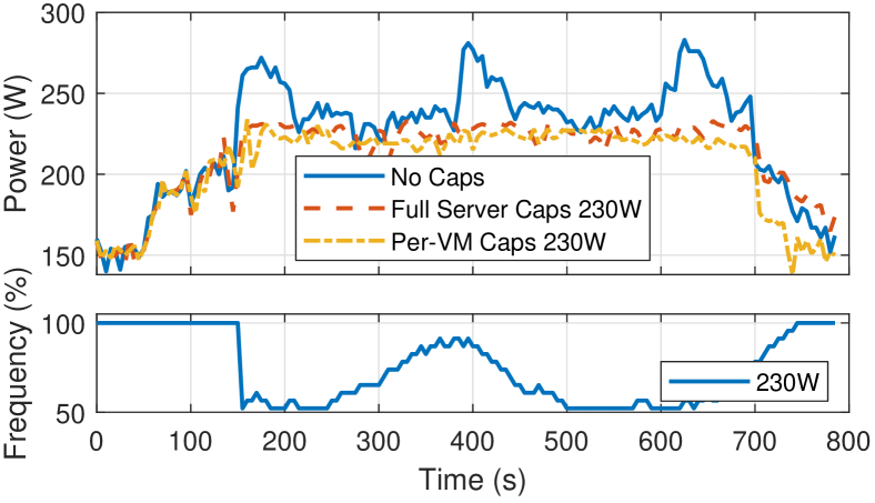
Figure 4: Server power dynamics.

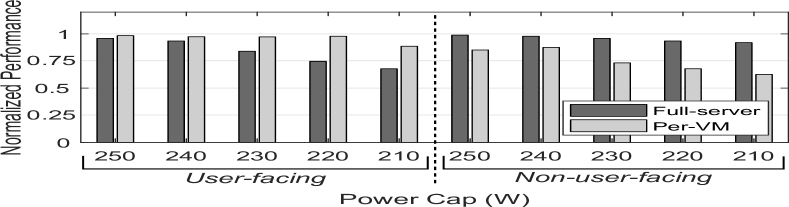
Figure 5: Performance impact of power capping.

The results show that full-server capping imposes a large tail latency degradation, especially for the lower caps. When the cap is 230W, the degradation is already 18%, which is often unacceptable for user-facing applications. For lower caps, full-server capping provides even worse tail latency (35% degradation for 210W). In contrast, our controller keeps tail latency very close to the unconstrained case, until the cap is so low (210W) that it becomes impossible to protect the user-facing application and RAPL needs to engage. This positive result comes at the cost of performance loss for the non-user-facing application. While full-server capping keeps running time fairly close to the unconstrained case, our controller degrades it by 28% for the 230W cap. This is the right tradeoff, as non-user-facing workloads have looser performance needs.

IV-D Chassis-level capping experiments

We now study the power draw at the chassis level, and the impact of different capping granularities (full-server vs per-VM) and VM placements. We experiment with a 12-server chassis running 36 copies of our user-facing application (each on a VM with 4 virtual cores), and 36 copies of our non-user-facing application (each running on a VM with 6 virtual cores). In terms of VM placement, we explore two extremes: (1) balanced placement, where we place the user-facing and non-user-facing VMs in round-robin fashion across the servers, i.e. 3 VMs of each type on each server; and (2) imbalanced, where we segregate user-facing and non-user-facing VMs on different sets of servers. Each experiment runs for 26 minutes.

Figure 6(left) plots the dynamic behavior of the chassis for an overall budget of 2450W for the two capping approaches. For comparison, we also plot the no-cap case. In these experiments, we use the balanced placement as an example.

As expected, both capping granularities are able to limit the power draw to the chassis budget, whereas the no-cap experiment substantially exceeds this value. We observe the same trends under the imbalanced placement approach. The VM placement does not matter in terms of the power profiles because the capping enforcement ensures no budget violations.

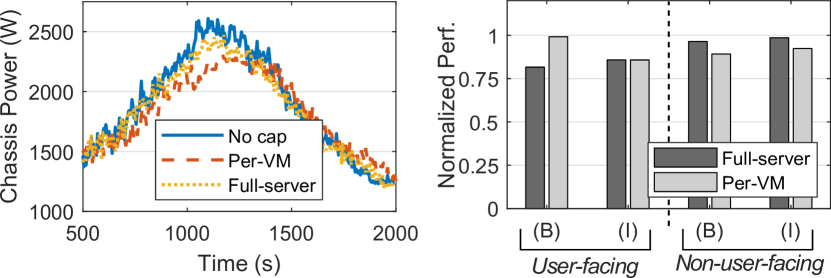
Figure 6: Chassis dynamics and performance vs placement.

However, VM placement has a large impact on application performance. Figure 6(right) plots the impact of VM placement and capping granularity on the average 95th-percentile latency of the user-facing applications (4 leftmost bars) and on the average running time of the non-user-facing applications (4 rightmost bars). We normalize to the no-cap results.

Per-VM capping under a balanced placement keeps the average tail latency the same as the no-cap experiment, despite the tight 2450W budget. In contrast, per-VM capping degrades performance as much as full-server capping when the placement is imbalanced. These results show that our controller protects user-facing VMs when the VM placement allows it.

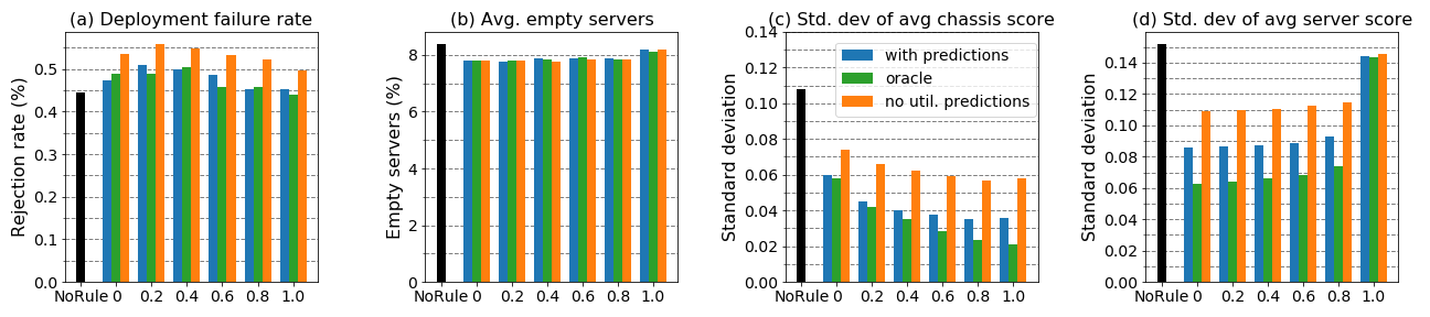
Figure 7: Key scheduler metrics, as a function of $\alpha$.

Full-server capping provides slightly better performance than per-VM capping for the non-user-facing applications. More interestingly, the results for balanced placement are slightly worse than for imbalanced placement, regardless of the capping granularity. For per-VM capping, the reason is that servers with only non-user-facing VMs need to reduce the frequency of fewer cores. For full-server capping, the reason is that servers with only non-user-facing VMs tend to have higher utilization, so a smaller reduction in frequency is enough for a large power reduction. Comparing the two rightmost bars, we see that full-server capping hurts performance slightly less than per-VM capping in the imbalanced case, as RAPL lowers frequency more slowly than our controller.

IV-E Cluster VM scheduler simulation

In the previous section, we explored extreme and manually-produced VM placements in controlled experiments. However, in practice, placements are determined by the VM scheduler. To evaluate our modified scheduler, we implement our VM placement policy in Azure’s VM scheduler, and simulate a cluster using 30 days of VM arrivals (Section IV-A). The simulator reports four main metrics:

• Deployment failure rate: the percent of VM deployment requests rejected by the scheduler due to resource unavailability or fragmentation. This rate has a direct impact on users, so our policy should not increase it;

• Average empty server ratio: the percent of servers without any VMs in the cluster averaged over time. Empty servers can accommodate the largest VM sizes, so our policy should not decrease this ratio;

• Standard deviation of the average chassis score, i.e. $1-(\rho^{Peak}/\rho^{Max})$ (Algorithm 1, line 13), for each chassis. This metric reflects how balanced the chassis are with respect to their power loads. Lower values are better and mean better balance and fewer power capping events;

• Standard deviation of the average server score, i.e. $(1/2)\times(1+(\gamma^{NUF}-\gamma^{UF})/N^{cores})$ (Algorithm 1, line 20), for each server. This metric reflects how balanced the servers are in terms of UF and NUF core 95th-percentile utilizations. Lower values mean better balance and that we are more likely to only need to cap NUF VMs.

Results. Figure 7 shows the results for these metrics, as a function of the $\alpha$ weight in our policy (Algorithm 1, line 6). $\alpha=1$ means that the server score is irrelevant, whereas $\alpha=0$ means that the chassis score is irrelevant. From left to right in each graph, the “NoRule” (black) bar represents the existing scheduler; the leftmost (blue) bar in each group represents our modified scheduler using our policy and ML predictions; the next (green) bar represents the modified scheduler using oracle predictions; and the rightmost (orange) the modified scheduler using criticality predictions, but no utilization predictions.

Comparing the black and blue bars illustrates the benefit of our policy and predictions. Figures 7(a) and (b) show that our modified scheduler impacts the failure rate slightly for low values of $\alpha$ (not at all for high values), while slightly decreasing the percentage of empty servers regardless of $\alpha$. The reason is that our policy may use a few more servers in the interest of better balancing the load. In fact, Figures 7(c) and (d) confirm that the load is more balanced using our policy and predictions. These latter graphs also show that the value of $\alpha$ is important. $\alpha=0$ produces much worse utilization balancing across chassis than other values. At the same time, $\alpha=1$ produces as poor server utilization balancing as the existing scheduler, whereas other values produce much better server balancing. These observations confirm that it is key to balance both across chassis and servers, as in our policy. $\alpha=0.8$ strikes a good compromise between the importance of these types of balancing.

Impact of prediction accuracy. Comparing the blue and green bars illustrates the impact of mispredictions and predictions with low confidence. Figures 7(c) and (d) show that oracle predictions produce only slightly better balancing than our real predictions for certain values of $\alpha$.

Impact of utilization predictions. Comparing the blue and orange bars illustrates the importance of having both criticality and utilization predictions. Clearly, it is critical to predict the workload type of each VM, as we want to protect the performance of user-facing VMs during capping events. The results demonstrate that having utilization predictions is also important. The lack of such predictions degrades the balancing substantially for most values of $\alpha$, and thus increases the capping rate and limits the power reduction during an event (thereby decreasing the potential for oversubscription).

IV-F Oversubscription increases

We now estimate the amount of oversubscription and dollar savings that result from our lower chassis power budgets. To do so, we translate the amount of budget we can reduce in each 60-chassis cluster into the infrastructure cost we would avoid. Oversubscription allows servers to be added to an existing datacenter (assuming space, cooling, and networking are available, as it is often the case), avoiding the cost of building a corresponding fraction of a new datacenter.

We instantiate our 5-step oversubscription strategy (Section III-E) with power telemetry from 1440 chassis over 3 months in 2018. We also use VM statistics from April 2019. Specifically, the 95th-percentile core utilizations for non-user-facing ($util_{NUF}$) and user-facing ($util_{UF}$) VMs were 44% and 65%, respectively, and the ratio of user-facing cores in the allocated cores ($\beta$) was 40%. We add a buffer of 10% to the chassis budget (step 5). For the results where providers treat external (i.e., third-party) VMs differently than internal (i.e., first-party) VMs, we adjust these parameters accordingly, while keeping the same amount of buffer.

Table IV lists results for several types of provisioning:

1. “Traditional” provisioning (no oversubscription);

2. State-of-the-art full-server capping without VM insights. In this approach, the power capping events need to be rare and the throttling has to be light to prevent performance loss to user-facing VMs. To model this approach with our provisioning strategy, we use $emax_{UF}+emax_{NUF}=$ 0.1%, $fmin_{UF}=fmin_{NUF}=$ 75%;

3. Predictions-based per-VM capping and scheduling, without impact on user-facing VMs. We use $emax_{UF}$ = 0, $fmin_{UF}$ = 100%, $emax_{NUF}$ = 1% and $fmin_{NUF}$ = 50%;

4. Predictions-based per-VM capping and scheduling, with minimal impact on user-facing VMs. To make this approach comparable to the others, we set the overall rate of capping events at 1%. Specifically, we use $emax_{UF}$ = 0.1%, $fmin_{UF}$ = 75%, $emax_{NUF}$ = 0.9% and $fmin_{NUF}$ = 50%;

5. Predictions-based per-VM capping and scheduling for internal VMs only (all external VMs considered user-facing), without impact on user-facing VMs;

6. Predictions-based per-VM capping and scheduling for internal VMs only (all external VMs considered user-facing), with minimal impact on user-facing VMs;

7. Predictions-based per-VM capping and scheduling for internal and non-premium external VMs, without impact on user-facing VMs; and

8. Predictions-based per-VM capping and scheduling for internal and non-premium external VMs, with minimal impact on user-facing VMs.

Approach	Chassis budget	Savings
	delta (%)	($10/W)
Traditional	0	0
State of the art	6.2%	$79.4M
Predictions for all VMs,
no UF impact	11.0%	$140.8M
Predictions for all VMs,
minimal UF impact	12.1%	$154.9M
Predictions for internal VMs,
no UF impact	8.4%	$107.5M
Predictions for internal VMs,
minimal UF impact	10.3%	$131.8M
Predictions for internal and
non-premium external VMs,
no UF impact	10.6%	$135.7M
Predictions for internal and
non-premium external VMs,
minimal UF impact	12.1%	$154.9M

TABLE IV: Comparison between provisioning approaches.

The state-of-the-art approach achieves 6.2% oversubscription. This amount is comparable to that (8%) achieved by Facebook [32], which knows the (single) workload that runs on each server. Public cloud platforms do not have this luxury.

In contrast, our approach (#3 and #4) can almost double the oversubscription and savings. We achieve more than 12% oversubscription with minimal impact on user-facing VMs. Assuming a datacenter campus of 128MW and an infrastructure cost of $10/W [2], 12.1% oversubscription translates into $154.9M in savings; an increase in savings of $75.5M over the state of the art. As providers can oversubscribe many campuses, the savings would be much higher in practice.

When providers prefer to treat external and internal VMs differently (approaches #5-#8), they can do so at the cost of a lower increase in oversubscription. For example, when treating all external VMs as user-facing and protecting the performance of user-facing VMs (#5), the increase in savings becomes $28.1M. At the other extreme, where we treat the premium external VMs as user-facing and allow minimal impact on user-facing VMs (#8), the increase in savings returns to $75.5M. The reason is that this provisioning approach has enough non-critical VMs, and oversubscription is limited only by the rate of capping events.

V Lessons from production deployment

So far, we have deployed our per-VM capping controller and ML models in production in Azure’s datacenters. Next, we discuss some of the lessons from these deployments.

Hypervisor support for per-VM power capping. Our prototype controller (Section III-D) leveraged the hypervisor’s core-grouping feature to manage the frequency of each VM’s physical cores. In production, Azure typically prefers not to restrict a VM to a subset of cores, so we could not rely on this feature. Instead, we had to extend the hypervisor to (1) add the capability to dynamically specify the frequency for a VM, and (2) carry the frequency to whichever cores it schedules the VM on during the context switch (changing the frequency takes tens of microseconds, whereas a scheduling quantum lasts 10 milliseconds). As most VMs are small (Table I), there was no need to manage frequency on a per-virtual-core basis.

Additional types of throttleable VMs. Some first-party customers were concerned about the impact of per-VM capping on their non-user-facing VMs. To alleviate their concerns, we added a configurable prioritized throttling list to our system. Using the list, we first consider low priority and internal non-production VMs for throttling and throttle production (including third-party, if configured) non-user-facing VMs as a last resort, i.e. when throttling the other types is insufficient.

Metrics to measure impact. Since VMs are black boxes, we cannot use any workload-specific metric to evaluate per-VM capping in production. Instead, our deployed system measures how long and how hard VMs are being capped. The data shows that our system is successful at protecting production user-facing VMs, while prioritizing the VMs that do get throttled.

Increasing rack density with per-VM capping. While deploying our system, we learned that Azure was installing fewer servers per rack – 28 instead of 36 – when deploying a new generation of power hungrier servers. Having fewer servers per rack reduces the probability that the rack power draw will hit the provisioned limit and cause capping using RAPL. With our per-VM capping system in place, Azure will go back to installing 36 servers per rack. This is another type of power oversubscription that per-VM capping enables.

Killing VMs. Some first-party customers indicated that they would prefer their VMs to be killed rather than throttled, as their services can handle losing VMs but an unpredictable impact due to throttling is not acceptable. Under extreme power draws, killing these customers’ VMs can help protect production user-facing VMs and throttle fewer non-user-facing ones. We will soon add this capability to our system.

Server support for per-VM management. Our production experience has highlighted the drawbacks of managing VM power per-component (e.g., core, uncore, memory). We expect that cloud providers would prefer to raise the level of abstraction from individual components to entire VMs, even if VM power would have to approximate. This would enable advances that have been too complex for production use, such as power-aware VM placement, enforcing per-VM power limits, and making capping and killing decisions based on VM power. We are working with silicon vendors towards this end.

VI Related Work

Our paper is the first to use ML predictions for increasing power oversubscription in public cloud platforms. Next, we discuss some of the most closely related works.

Leveraging predictions. Some works predict resource demand, resource utilization, or job/task length for provisioning or scheduling purposes, e.g. [5, 6, 10, 16, 17, 28]. In contrast, we introduce a new algorithm and ML models for predicting workload type and high-percentile utilization, seeking to protect critical workloads from capping and place VMs in a criticality- and capping-aware manner.

Server power capping. Most efforts have focused on selecting the DVFS setting required to meet a tight power budget as applications execute, e.g. [13, 15, 20, 22, 23, 24, 25, 27, 34]. Both modeling/optimization and feedback techniques have been used. The inputs to the selection have been either application-level metrics (e.g., request latency), low-level performance counters, or operator annotations (e.g., high priority application). Our capping controller uses per-core DVFS and feedback, so it adds to this body of work. However, it also uses predictions about the VMs’ performance-criticality as its inputs. Our approach seems to be the best for a cloud platform, since criticality information and application-level metrics are typically not available, and collecting and tracking low-level counters at scale involves undesirable overhead.

Cluster-wide workload placement/scheduling. Many works select workload placements to reduce performance interference or energy usage, e.g. [3, 4, 8, 26, 30, 33]. Unfortunately, they are often impractical for a cloud provider, relying on extensive profiling, application-level metrics, short-term load predictions, and/or aggressive resource reallocation (e.g., via live migration). Live migration is particularly problematic, as it retains contended resources, may produce traffic bursts, and may impact VM availability; it is better to place VMs where they can stay. Our scheduler uses predictions in VM placement. Unlike prior work, it reduces the number and impact of capping events, and increases power oversubscription.

Datacenter oversubscription. Researchers have proposed to use statistical oversubscription, where one profiles the aggregate power draw of multiple services and deploy them to prevent correlated peaks [9, 11, 14, 31]. Our work extends these works by using predictions to place the workload, inform capping, and increase oversubscription. Our oversubscription strategy is also the first to carefully control the extent and impact of capping on important cloud workloads.

Others have studied hierarchical capping in production datacenters [9, 14, 32]. Our paper focuses on chassis-level power budget enforcement to make our experimentation easier. However, our techniques extrapolate directly. For example, for row-level budget enforcement, we can place VMs across rows trying to balance rows and servers.

Finally, researchers have proposed using energy storage to shave power peaks in oversubscribed datacenters [12, 18]. When peaks last long, this approach may require large amounts of storage, which our work does not require. Nevertheless, the two approaches are orthogonal and can be combined.

VII Conclusions

We proposed prediction-based techniques for increasing power oversubscription in cloud platforms, while protecting important workloads. Our techniques can increase oversubscription by $2\times$. We discussed lessons from deploying our techniques in production. We conclude that recent advances in ML and prediction-serving systems can unleash further innovations in cloud resource provisioning and management.

References

- [1] S. I. Abrita, M. Sarker, F. Abrar, and M. A. Adnan, “Benchmarking vm startup time in the cloud,” in Benchmarking, Measuring, and Optimizing, C. Zheng and J. Zhan, Eds. Cham: Springer International Publishing, 2019, pp. 53–64.
- [2] L. A. Barroso, U. Hölzle, and P. Ranganathan, “The datacenter as a computer: Designing warehouse-scale machines,” Synthesis Lectures on Computer Architecture, vol. 13, no. 3, 2018.
- [3] A. Beloglazov and R. Buyya, “Energy Efficient Resource Management in Virtualized Cloud Data Centers,” in Proceedings of the 10th International Conference on Cluster, Cloud and Grid Computing, 2010.
- [4] N. Bobroff, A. Kochut, and K. Beaty, “Dynamic Placement of Virtual Machines for Managing SLA Violations,” in Proceedings of the International Symposium on Integrated Network Management, 2007.
- [5] R. N. Calheiros, E. Masoumi, R. Ranjan, and R. Buyya, “Workload Prediction Using ARIMA Model and its Impact on Cloud Applications’ QoS,” IEEE Transactions on Cloud Computing, vol. 3, no. 4, 2015.
- [6] E. Cortez, A. Bonde, A. Muzio, M. Russinovich, M. Fontoura, and R. Bianchini, “Resource central: Understanding and predicting workloads for improved resource management in large cloud platforms,” in Proceedings of the 26th Symposium on Operating Systems Principles, 2017.
- [7] H. David, E. Gorbatov, U. R. Hanebutte, R. Khanna, and C. Le, “RAPL: Memory Power Estimation And Capping,” in Proceedings of the International Symposium on Low-Power Electronics and Design, 2010.
- [8] C. Delimitrou and C. Kozyrakis, “Quasar: Resource-Efficient and QoS-Aware Cluster Management,” in Proceedings of the 19th International Conference on Architectural Support for Programming Languages and Operating Systems, 2014.
- [9] X. Fan, W.-D. Weber, and L. A. Barroso, “Power provisioning for a warehouse-sized computer,” in Proceedings of the 34th Annual International Symposium on Computer Architecture, 2007.
- [10] Z. Gong, X. Gu, and J. Wilkes, “Press: Predictive Elastic Resource Scaling for Cloud Systems,” in Proceedings of the International Conference on Network and Service Management, 2010.
- [11] S. Govindan, J. Choi, B. Urgaonkar, A. Sivasubramaniam, and A. Baldini, “Statistical profiling-based techniques for effective power provisioning in data centers,” in Proceedings of the 4th ACM European conference on Computer systems, 2009.
- [12] S. Govindan, D. Wang, A. Sivasubramaniam, and B. Urgaonkar, “Leveraging stored energy for handling power emergencies in aggressively provisioned datacenters,” SIGARCH Comput. Archit. News, vol. 40, no. 1, 2012.
- [13] A. Guliani and M. M. Swift, “Per-Application Power Delivery,” in Proceedings of Eurosys, 2019.
- [14] C.-H. Hsu, Q. Deng, J. Mars, and L. Tang, “Smoothoperator: Reducing power fragmentation and improving power utilization in large-scale datacenters,” in Proceedings of the 23rd International Conference on Architectural Support for Programming Languages and Operating Systems, 2018.
- [15] C. Isci, A. Buyuktosunoglu, C.-Y. Cher, P. Bose, and M. Martonosi, “An analysis of efficient multi-core global power management policies: Maximizing performance for a given power budget,” in Proceedings of the 39th annual IEEE/ACM international symposium on microarchitecture, 2006.
- [16] S. Islam, J. Keung, K. Lee, and A. Liu, “Empirical Prediction Models for Adaptive Resource Provisioning in the Cloud,” Future Generation Computer Systems, vol. 28, no. 1, 2012.
- [17] A. Khan, X. Yan, S. Tao, and N. Anerousis, “Workload Characterization and Prediction in the Cloud: A Multiple Time Series Approach,” in Proceedings of the International Conference on Network and Service Management, 2012.
- [18] V. Kontorinis, L. E. Zhang, B. Aksanli, J. Sampson, H. Homayoun, E. Pettis, D. M. Tullsen, and T. S. Rosing, “Managing distributed ups energy for effective power capping in data centers,” in Proceedings of the 39th International Symposium on Computer Architecture, 2012.
- [19] K. Lange, “Identifying shades of green: The specpower benchmarks,” Computer, vol. 42, 2009.
- [20] C. Lefurgy, X. Wang, and M. Ware, “Server-level power control,” in Proceedings of the 4th International Conference on Autonomic Computing, 2007.
- [21] Y. Li, C. R. Lefurgy, K. Rajamani, M. S. Allen-Ware, G. J. Silva, D. D. Heimsoth, S. Ghose, and O. Mutlu, “A Scalable Priority-Aware Approach to Managing Data Center Server Power,” in Proceedings of the International Symposium on High Performance Computer Architecture, 2019.
- [22] Y. Liu, G. Cox, Q. Deng, S. C. Draper, and R. Bianchini, “Fastcap: An efficient and fair algorithm for power capping in many-core systems,” in Proceedings of the IEEE International Symposium on Performance Analysis of Systems and Software, 2016.
- [23] D. Lo, L. Cheng, R. Govindaraju, P. Ranganathan, and C. Kozyrakis, “Heracles: Improving Resource Efficiency at Scale,” in ACM SIGARCH Computer Architecture News, vol. 43, no. 3, 2015, pp. 450–462.
- [24] K. Ma, X. Li, M. Chen, and X. Wang, “Scalable power control for many-core architectures running multi-threaded applications,” ACM SIGARCH Computer Architecture News, vol. 39, no. 3, 2011.
- [25] A. K. Mishra, S. Srikantaiah, M. Kandemir, and C. R. Das, “Cpm in cmps: Coordinated power management in chip-multiprocessors,” in Proceedings of the ACM/IEEE International Conference for High Performance Computing, Networking, Storage and Analysis, 2010.
- [26] D. Novakovic, N. Vasic, S. Novakovic, D. Kostic, and R. Bianchini, “DeepDive: Transparently Identifying and Managing Performance Interference in Virtualized Environments,” in Proceedings of the USENIX Annual Technical Conference, 2013.
- [27] R. Raghavendra, P. Ranganathan, V. Talwar, Z. Wang, and X. Zhu, “No ”power” struggles: Coordinated multi-level power management for the data center,” in Proceedings of the 13th International Conference on Architectural Support for Programming Languages and Operating Systems, 2008.
- [28] N. Roy, A. Dubey, and A. Gokhale, “Efficient Autoscaling in the Cloud Using Predictive Models for Workload Forecasting,” in Proceedings of the International Conference on Cloud Computing, 2011.
- [29] R. Sakamoto, T. Cao, M. Kondo, K. Inoue, M. Ueda, T. Patki, D. Ellsworth, B. Rountree, and M. Schulz, “Production Hardware Overprovisioning: Real-world Performance Optimization Using an Extensible Power-Aware Resource Management Framework,” in Proceedings of the International Parallel and Distributed Processing Symposium, 2017.
- [30] A. Verma, P. Ahuja, and A. Neogi, “pMapper: Power and Migration Cost Aware Application Placement in Virtualized Systems,” in Proceedings of the International Conference on Distributed Systems Platforms and Open Distributed Processing, 2008.
- [31] G. Wang, S. Wang, B. Luo, W. Shi, Y. Zhu, W. Yang, D. Hu, L. Huang, X. Jin, and W. Xu, “Increasing large-scale data center capacity by statistical power control,” in Proceedings of the 11th European Conference on Computer Systems, 2016.
- [32] Q. Wu, Q. Deng, L. Ganesh, C.-H. Hsu, Y. Jin, S. Kumar, B. Li, J. Meza, and Y. J. Song, “Dynamo: Facebook’s data center-wide power management system,” in Proceedings of the 43rd International Symposium on Computer Architecture, 2016.
- [33] H. Yang, A. Breslow, J. Mars, and L. Tang, “Bubble-flux: Precise Online QoS Management for Increased Utilization in Warehouse Scale Computers,” in Proceedings of the 40th Annual International Symposium on Computer Architecture, 2013.
- [34] H. Zhang and H. Hoffmann, “Maximizing Performance Under a Power Cap: A Comparison of Hardware, Software, and Hybrid Techniques,” in Proceedings of the International Conference on Architectural Support for Programming Languages and Operating Systems, 2016.