Learning Centric Wireless Resource Allocation for Edge Computing: Algorithm and Experiment

Abstract

Edge intelligence is an emerging network architecture that integrates sensing, communication, computing components, and supports various machine learning applications, where a fundamental communication question is: how to allocate the limited wireless resources (such as time, energy) to the simultaneous model training of heterogeneous learning tasks? Existing methods ignore two important facts: 1) different models have heterogeneous demands on training data; 2) there is a mismatch between the simulated environment and the real-world environment. As a result, they could lead to low learning performance in practice. This paper proposes the learning centric wireless resource allocation (LCWRA) scheme that maximizes the worst learning performance of multiple tasks. Analysis shows that the optimal transmission time has an inverse power relationship with respect to the generalization error. Finally, both simulation and experimental results are provided to verify the performance of the proposed LCWRA scheme and its robustness in real implementation.

I Introduction

Edge computing has been proposed in recent years as a solution to the high transmission cost in cloud computing and limited performance in local computing [1]. It pushes the cloud services from the network core to the network edges that are in closer proximity to Internet of Things (IoT) devices [2]. With the edge computing platform, various machine learning applications can reside at the edge, giving rise to an emerging paradigm termed edge intelligence [3]. Edge intelligence can be divided into edge model training and edge model inference. In general, there are two ways to implement edge model training: centralized training and distributed training. Centralized training collects sensing data generated from IoT devices and trains the learning models at the edge [4, 5]. Distributed training deploys individual learning models at user terminals, and all the users upload their local model parameters periodically to the edge for model aggregation and broadcasting [6]. Since the IoT devices usually can hardly process the data due to limited computation power, this paper focuses on centralized training.

In centralized training, a fundamental communication question is: how to allocate the limited wireless resources (such as time, energy) to train multiple learning tasks simultaneously? Existing methods such as the time fairness scheme, the throughput fairness scheme [7], or the importance-aware transmission scheme [8, 9] ignore the heterogeneous requests of learning tasks on the data amount, probably leading to low learning performance. Furthermore, all these schemes are verified only via computer simulation. Due to the transmission overhead of control signals [10] (which results in reduced number of useful data) and random nature of wireless channels [11] (e.g., disconnection/reconnection procedures), there is a mismatch between the simulated environment and the real-world environment. Therefore, apart from computer simulation, hardware experiments are required to demonstrate the robustness of resource allocation algorithms against practical uncertainties.

To address the above problems, this paper adopts the statistical mechanics of learning [14] to predict the learning accuracy of different tasks versus the amount of training data, and reveal the relationship between the learning performance and the wireless resources/channels. By leveraging the difference of convex programming (DCP), a learning centric wireless resource allocation (LCWRA) maximizing the learning performance is proposed. Analysis shows that the optimal transmission time has an inverse power relationship with respect to the generalization error. This empowers us to use a ranking-based procedure to derive the optimal time when the network energy is unlimited. Simulation results are provided to verify the performance of the proposed LCWRA scheme. Experimental results for robotic image dataset collection and vehicular point-cloud dataset collection are further carried out to demonstrate the effectiveness and robustness of LCWRA in real systems.

II System Model and Problem Formulation

Consider an edge intelligence system consisting of one server and $K$ users with dataset $\left\{\mathcal{D}_{1},\cdots,\mathcal{D}_{K}\right\}$. There are $M$ learning models to be trained at the edge, and let $\mathcal{Y}_{m}\in\left\{\mathcal{Y}_{1},\cdots,\mathcal{Y}_{M}\right\}$ denote the users who transmit training samples for the model $m\in\{1,\cdots,M\}$. The total number of training samples for model $m$ collected at the edge is

$$v_{m}=\sum_{k\in\mathcal{Y}_{m}}\left\lfloor\frac{d_{k}}{D_{k}}\right\rfloor+c_{m}\approx\sum_{k\in\mathcal{Y}_{m}}\frac{d_{k}}{D_{k}}+c_{m},$$ (1)

where $d_{k}$ represents the data amount transmitted by user $k\in\{1,\cdots,K\}$, $D_{k}$ represents the data size per sample, and $c_{m}$ denotes the number of historical samples available at the edge for model $m$. The approximation is based on $\lfloor x\rfloor\approx x$ when $x\gg 1$. In this paper, it is assumed that the datasets $\left\{\mathcal{D}_{1},\cdots,\mathcal{D}_{K}\right\}$ are independent and identically distributed. Therefore, the generalization error, denoted as $\Psi_{m}$ is a function of the number of samples $v_{m}$. To the best of the authors’ knowledge, there is no exact expression of $\Psi_{m}(v_{m})$. To this end, an inverse power law model [4, 5, 12, 13], which is supported by statistical mechanics of learning [14], is adopted to approximate $\Psi_{m}$ as

$$\Psi_{m}\approx a_{m}\,v_{m}^{-b_{m}},$$ (2)

where $a_{m},b_{m}>0$ are tuning parameters.

Our aim is to minimize $\{\Psi_{m}{|\forall m}\}$ by proper wireless resource allocations. Specifically, we consider the sample transmission in a single-hop time division multiple access (TDMA)-based wireless system. Within a period of $T_{\rm{max}}$, the user $k$ is assigned a duration of $t_{k}\in\mathbb{R}_{+}$ to transmit samples. As a result, the data amount transmitted by user $k$ is

$$d_{k}=t_{k}R_{k},$$ (3)

where $R_{k}$ represents the data-rate of user $k$. Since the network adopts the TDMA, the transmission of each user is scheduled by a wireless controller and therefore the transmission is collision-free[15]. Therefore, $R_{k}$ is determined by the bandwidth $B$ allocated to the system and the signal-to-noise ratio at user $k$, i.e.,

$$R_{k} =B\log_{2}\left(1+\frac{|h_{k}|^{2}E_{k}}{t_{k}\sigma^{2}}\right),$$ (4)

where $E_{k}\in\mathbb{R}_{+}$ represents the transmit energy at user $k$, $h_{k}\in\mathbb{C}$ represents the channel between the user $k$ and the edge, and $\sigma^{2}$ denotes the power of Gaussian white noise. Hence, the transmit power at user $k$ is $E_{k}/t_{k}$. The transmit power is limited by the hardware structure as $E_{k}/t_{k}\leq P_{\rm{max}}$, where $P_{\rm{max}}$ denotes the peak power. In applications such as sensor networks, the total energy is usually limited by an upper bound $E_{\mathrm{max}}$ for the consideration of energy efficiency [18], which gives $\sum_{k=1}^{K}E_{k}\leq E_{\rm{max}}$.

In the considered edge computing system driven by learning tasks, the aim is to minimize generalization errors subject to communication constraints, which leads to the following optimization problem.

$$\textrm{P}1:\quad \min_{\vec{\mathbf{t}},\vec{\mathbf{e}}}~{}\max_{m=1,\cdots,M}$$

$$\left\{a_{m}\left(\sum_{k\in\mathcal{Y}_{m}}\frac{t_{k}B}{D_{k}}\log_{2}\left(1+\frac{E_{k}|h_{k}|^{2}}{t_{k}\sigma^{2}}\right)+c_{m}\right)^{-b_{m}}\right\},$$

s.t. $$\sum_{k=1}^{K}t_{k}\leq T_{\textrm{max}},\quad\sum_{k=1}^{K}E_{k}\leq E_{\textrm{max}},$$ (5a)

$$\frac{E_{k}}{t_{k}}\leq P_{\rm{max}},\quad\forall k,$$ (5b)

$$\frac{t_{k}B}{D_{k}}\log_{2}\left(1+\frac{E_{k}|h_{k}|^{2}}{t_{k}\sigma^{2}}\right)\leq|\mathcal{D}_{k}|,\quad\forall k,$$ (5c)

$$t_{k}\geq 0,\ E_{k}\geq 0,\quad\forall k,$$ (5d)

where the min-max operation in the objective function aims to warrant the worst learning performance of all models, $\vec{\mathbf{t}}=[t_{1},\cdots,t_{K}]^{T}$ and $\vec{\mathbf{e}}=[E_{1},\cdots,E_{K}]^{T}$.

Use Case (Vehicular Point-Cloud Dataset Collection): For autonomous vehicles, object detection based on artificial intelligence (AI) models is needed for collision avoidance [19, 20]. To train AI models, AI companies (e.g., Google, Baidu) arrange vehicles to collect sensing data in various environment (as shown in Fig. 1). The time is limited as the sensing data is massive. Thus data selection and vehicular wireless resource allocation are required. After data transmission, the data is manually annotated and used for training AI models [21].

Figure 1: The use case of vehicular point-cloud dataset collection.

III DCP-based LCWRA Algorithm

For notation convenience, we first define function

$$d_{k}=\Theta_{k}(t_{k},E_{k})=t_{k}B\log_{2}\left(1+E_{k}|h_{k}|^{2}/(t_{k}\sigma^{2})\right).$$ (6)

As $\Theta_{k}(t_{k},E_{k})$ is the perspective transformation of logarithm function $B\log_{2}\left(1+E_{k}|h_{k}|^{2}/\sigma^{2}\right)$ with respect to $t_{k}$, it is concave with respect to both $t_{k}$ and $E_{k}$. On the other hand, as $a_{m}>0$ and $b_{m}>0$, $a_{m}\,x^{-b_{m}}$ is a decreasing and convex function of $x$. According to the composition law [22], $a_{m}\left(\sum_{k\in\mathcal{Y}_{m}}\Theta_{k}(t_{k},E_{k})/D_{k}+c_{m}\right)^{-b_{m}}$ is convex with respect to $\{t_{k}|\forall k\}$ and $\{E_{k}|\forall k\}$ . Because a point-wise maximum over a group of convex functions is convex, the objective function of P1 is convex. Adding to the fact that constraints (5a), (5b), and (5d) are all linear, the only nonconvex part in P1 is the constraint (5c).

To address the nonconvexity of (5c), we leverage difference of convex programming (DCP) [23] to replace the left side of constraint (5c) with its first order Taylor Expansion, which is an upper bound. Specifically, for any feasible solution $\vec{\mathbf{x}}^{\diamond}=\left[t_{k}^{\diamond},E_{k}^{\diamond}\right]^{T}$ of P1, we define the first order Taylor Expansion of $\Theta_{k}$ as a surrogate function $\widehat{\Theta}_{k}$:

$$\widehat{\Theta}_{k}(\vec{\mathbf{x}}|\vec{\mathbf{x}}^{\diamond})=\Theta_{k}\left(\vec{\mathbf{x}}^{\diamond}\right)+\left(\vec{\mathbf{x}}-\vec{\mathbf{x}}^{\diamond}\right)^{T}\nabla\Theta_{k}\left(\vec{\mathbf{x}}^{\diamond}\right).$$ (7)

Since $\Theta_{k}$ is a concave function, we have $\widehat{\Theta}_{k}(\vec{\mathbf{x}}|\vec{\mathbf{x}}^{\diamond})\geq\Theta_{k}(\vec{\mathbf{x}})$. Therefore, we can replace $\Theta_{k}$ in (5c) with $\widehat{\Theta}_{k}$ at a feasible point $\vec{\mathbf{x}}^{\diamond}=\{\vec{\mathbf{t}}^{\diamond},\vec{\mathbf{e}}^{\diamond}\}$ and formulate a surrogate problem of P1. Since the feasible set has shrunk, the surrogate problem would generate another feasible solution $\vec{\mathbf{x}}^{\prime}$, which can be used to derive a tighter surrogate problem. This leads to an iterative refinement procedure as follows: with an initial feasible solution $\vec{\mathbf{x}}^{(0)}=\left\{\vec{\mathbf{t}}^{(0)},\vec{\mathbf{e}}^{(0)}\right\}$, we update $\vec{\mathbf{x}}^{(n)}$ at the $n$-th iteration as

$$\vec{\mathbf{x}}^{(n)}=\left\{\vec{\mathbf{t}}^{(n)},\vec{\mathbf{e}}^{(n)}\right\}$$ (8)

$$=\arg\min_{\vec{\mathbf{t}},\vec{\mathbf{e}}}\max_{m}~{}\left\{a_{m}\left(\sum_{k\in\mathcal{Y}_{m}}\frac{\Theta_{k}(t_{k},E_{k})}{D_{k}}+c_{m}\right)^{-b_{m}}\right\}$$

under the constraints of (5a), (5b), (5d) and

$$\widehat{\Theta}_{k}(t_{k},E_{k}|t_{k}^{(n-1)},E_{k}^{(n-1)})/D_{k}\leq|\mathcal{D}_{k}|,\quad\forall k.$$ (9)

The above problem is convex, which can be readily solved by CVX software [22]. The entire iterative procedure is termed DCP-based LCWRA, and its convergence property is summarized below.

Theorem 1.

If $\vec{\mathbf{x}}^{\diamond(0)}$ is a feasible solution to P1, any limit point $\vec{\mathbf{x}}^{*}$ of the sequence $\left\{\vec{\mathbf{x}}^{\diamond(0)},\vec{\mathbf{x}}^{\diamond(1)},\cdots\right\}$ is Karush-Kuhn-Tucher solution to problem P1.

Proof.

It can be shown that $\widehat{\Theta}_{k}(\vec{\mathbf{x}}^{*}|\vec{\mathbf{x}}^{*})=\Theta_{k}(\vec{\mathbf{x}}^{*})$ and $\nabla\widehat{\Theta}_{k}(\vec{\mathbf{x}}^{*}|\vec{\mathbf{x}}^{*})=\nabla\Theta_{k}(\vec{\mathbf{x}}^{*})$. Combining the above results and $\widehat{\Theta}_{k}(\vec{\mathbf{x}}|\vec{\mathbf{x}}^{*})\geq\Theta_{k}(\vec{\mathbf{x}})$, and according to [23], the theorem is immediately proved. ∎

IV Ranking-Based LCWRA

In the previous section, problem P1 is solved numerically. In order to obtain insights on how learning tasks influence the resource allocation strategy, an analytical solution is derived in this section. In particular, it is assumed that $E_{\rm{max}}$ is sufficiently large such that $E_{\rm{max}}\geq T_{\rm{max}}P_{\rm{max}}$. Then, all users will transmit with their maximum power, i.e., $E_{k}/t_{k}=P_{\rm{max}}$, and the constraints (5b) and second part of (5a) are removed. The data-rate is fixed to $R_{k}=B\log_{2}\left(1+P_{\rm{max}}|h_{k}|^{2}/\sigma^{2}\right)$. Therefore, problem P1 with large $E_{\rm{max}}$ is given by

$$\textrm{P}2:\min_{\vec{\mathbf{t}},u}~{}~{} u,$$

s.t. $$u\geq a_{m}\Big{(}\sum_{k\in\mathcal{Y}_{m}}\frac{t_{k}R_{k}}{D_{k}}+c_{m}\Big{)}^{-b_{m}},\quad\forall m,$$ (10a)

$$\sum_{k=1}^{K}t_{k}\leq T_{\textrm{max}},$$ (10b)

$$\frac{t_{k}R_{k}}{D_{k}}\leq|\mathcal{D}_{k}|,\ t_{k}\geq 0,\quad\forall k,$$ (10c)

where $u$ is a slack variable denoting the level of generalization error. An efficient way to determine the optimal $u$, denoted as $u^{*}$ in $\mathrm{P}2$ is to use bisection algorithm. Specifically, given an upper bound for the searching interval, say $u_{\mathrm{max}}$, and a lower bound $u_{\mathrm{min}}$, the trial point is set to $u^{\diamond}=(u_{\mathrm{max}}+u_{\mathrm{min}})/2$. If $\mathrm{P}2$ with $u=u^{\diamond}$ is feasible, the upper bound is updated as $u_{\mathrm{max}}=u^{\diamond}$; otherwise, the lower bound is updated as $u_{\mathrm{min}}=u^{\diamond}$. The process is repeated until $|u_{\mathrm{max}}-u^{\diamond}|<\epsilon$, where $\epsilon$ is a small positive constant to control the accuracy. Initially, we set $u_{\mathrm{max}}=1$ and $u_{\mathrm{min}}=0$.

Now the remaining question is how to provide a feasibility check of $\mathrm{P}2$ given $u=u^{\diamond}$. To this end, we first minimize the transmission time via the following problem:

$$\textrm{P}3:\min_{\vec{\mathbf{t}}}~{}~{} \sum_{k=1}^{K}t_{k},$$

s.t. $$\sum_{k\in\mathcal{Y}_{m}}\frac{t_{k}R_{k}}{D_{k}}\geq\left(\frac{u^{\diamond}}{a_{m}}\right)^{-\frac{1}{b_{m}}}-c_{m},\quad\forall m,$$ (11a)

$$\frac{t_{k}R_{k}}{D_{k}}\leq|\mathcal{D}_{k}|,\ t_{k}\geq 0,\quad\forall k,,$$ (11b)

and then check if $\sum_{k=1}^{K}t_{k}^{*}\leq T_{\rm{max}}$. If so, problem $\mathrm{P}2$ with $u=u^{\diamond}$ is feasible; otherwise, the time budget cannot support learning performance $u^{\diamond}$ and $\mathrm{P}2$ with $u=u^{\diamond}$ is infeasible.

The transformation from $\mathrm{P}2$ to $\mathrm{P}3$ via bisection allows us to decouple the time variables among different groups. In other words, $\mathrm{P}3$ can be readily decomposed into subproblems $\mathrm{P}3[1],\cdots,\mathrm{P}3[M]$ for all the learning models respectively, and each $\mathrm{P}3[m]$ can be solved analytically by a ranking-based procedure. More specifically, define $U_{i,m}=R_{k}/D_{k}$, $V_{i,m}=|\mathcal{D}_{k}|$, and $z_{i,m}=t_{k}$, where $k\in\mathcal{Y}_{m}$ and $R_{k}/D_{k}$ is the $i$-th largest element in the set $\{R_{k}/D_{k},k\in\mathcal{Y}_{m}\}$. Then finding the optimal $t_{k}$ is equivalent to finding the optimal $z_{i,m}$, which can be achieved by solving the following problem.

$$\textrm{P}3[m]:\min_{\{z_{i,m}\}}\quad \sum_{i=1}^{|\mathcal{Y}_{m}|}z_{i,m},$$

s.t. $$\sum_{i=1}^{|\mathcal{Y}_{m}|}U_{i,m}z_{i,m}\geq\left(\frac{u^{\diamond}}{a_{m}}\right)^{-\frac{1}{b_{m}}}-c_{m},$$ (12a)

$$U_{i,m}z_{i,m}\leq V_{i,m},\quad i=1,...,|\mathcal{Y}_{m}|,$$ (12b)

$$z_{i,m}\geq 0,\quad i=1,...,|\mathcal{Y}_{m}|.$$ (12c)

The optimal solution to $\textrm{P}3[m]$ is summarized in the following theorem.

Theorem 2.

The optimal solution $z^{*}_{i,m}$ to $\textrm{P}3[m]$ is $z^{*}_{i,m}(u^{\diamond})=0$ if $\left(u^{\diamond}/a_{m}\right)^{-\frac{1}{b_{m}}}-c_{m}\leq 0$. Otherwise,

$$z^{*}_{i,m}(u^{\diamond})=$$

$$\frac{\min\left(V_{i,m},\left(\frac{u^{\diamond}}{a_{m}}\right)^{-\frac{1}{b_{m}}}-c_{m}-\sum_{j=1}^{i-1}U_{j,m}z^{*}_{j,m}(u^{\diamond})\right)}{U_{i,m}}.$$ (13)

Proof.

See [24, Appendix A]. ∎

According to Theorem 2, if $k=\arg\max_{j\in\mathcal{Y}_{m}}R_{j}$, we can set $i=1$ in (13), which gives

$$t^{*}_{k}={\frac{D_{k}}{R_{k}}}\min\left\{|\mathcal{D}_{k}|,\left(\frac{u^{\diamond}}{a_{m}}\right)^{-\frac{1}{b_{m}}}-c_{m}\right\},$$ (14)

This proves an inverse power relationship between the transmission time and the learning error $u^{\diamond}$. On the other hand, if $k\neq\arg\max_{j\in\mathcal{Y}_{m}}R_{j}$, we need to compute the required number of samples $\left(u^{\diamond}/a_{m}\right)^{-\frac{1}{b_{m}}}$ for task $m$, and then subtract the number of samples transmitted by other users in group $\mathcal{Y}_{m}$ with higher data-rates than $R_{k}$. In other words, the optimal time of a particular user $k$ would not be affected by the users in other groups or those in the same group but with lower data-rates than $R_{k}$. Therefore, the entire algorithm for solving $\rm{P}2$ based on Theorem 2 is termed ranking-based LCWRA.

V Simulation Results

In this section, simulation results are provided to verify the performance of the proposed algorithms. We consider the case of $K=4$ and $M=2$ with $\mathcal{Y}_{1}=\{1\}$ and $\mathcal{Y}_{2}=\{2,3,4\}$, where the first task is to classify MNIST dataset [25] via convolutional neural network (CNN), and the second task is to classify digits dataset in Scikit-learn [26] via support vector machine (SVM). For CNN, it has $6$ layers (as shown in Fig. 1 in [4]), and the training procedure is implemented via Adam optimizer with a learning rate of $10^{-4}$ and a mini-batch size of $100$. For SVM, it uses penalty coefficient $C=1$ and Gaussian kernel function $K(\mathbf{x}_{i},\mathbf{x}_{j})=\mathrm{exp}\left(-\widetilde{\gamma}\,\|\mathbf{x}_{i}-\mathbf{x}_{j}\|_{2}^{2}\right)$ with $\widetilde{\gamma}=0.001$. The data size of each sample is $D_{1}=6276~{}\mathrm{bits}$ for the MNIST dataset and $D_{2}=324~{}\mathrm{bits}$ for the digits dataset in Scikit-learn. It is assumed that there are $A_{1}=300$ CNN samples and $A_{2}=200$ SVM samples in the historical dataset. The bandwidth $B=180~{}\mathrm{kHz}$ [28]. The channel of user $k$ is generated according to $\mathcal{CN}(0,\varrho)$ where $\varrho=-90~{}\rm{dB}$ is the path loss [27], and the noise power is set as $-130~{}\rm{dBm/Hz}$. The simulation is repeated with $10$ independent channels, and each point in the figure is generated by averaging the $10$ monte-carlo runs.

The tuning parameters $\{a_{m}\}$ and $\{b_{m}\}$ are fitted using MNIST dataset and the digit dataset in Scikit-learn toolbox, respectively. For CNN, we vary the sample size $v_{1}$ as $(v^{(1)}_{1},v^{(2)}_{1},\cdots)=(100,150,200,300)$ and train the CNN for $5000$ iterations. The classification errors on a test dataset with another $1000$ MNIST samples are given by $(0.2970,0.2330,0.2150,0.1180)$. For SVM, we vary the sample size $v_{1}$ as $(v^{(1)}_{1},v^{(2)}_{1},\cdots)=(30,50,100,200)$. The classification errors on a test dataset with another $797$ samples are given by $(0.4774,0.2513,0.2010,0.1445)$. Via the nonlinear least squares fitting, we have $(a_{1},b_{1})=(7.3,0.69)$ and $(a_{2},b_{2})=(6.24,0.72)$. In practice, $\{a_{m},b_{m}\}$ are estimated via extrapolation of learning curves [12, 13] and exact $\left\{a_{m},b_{m}\right\}$ is not available. To this end, we also consider the practical LCWRA scheme with estimation errors of $(a_{m},b_{m})$ being $10\%$, i.e., $a_{1}\sim\mathcal{U}(7.3-0.73,7.3+0.73),b_{1}\sim\mathcal{U}(0.69-0.069,0.69+0.069)$, $a_{2}\sim\mathcal{U}(6.24-0.624,6.24+0.624),b_{2}\sim\mathcal{U}(0.72-0.072,0.72+0.072)$, where $\mathcal{U}(x,y)$ represents uniform distribution within $[x,y]$.

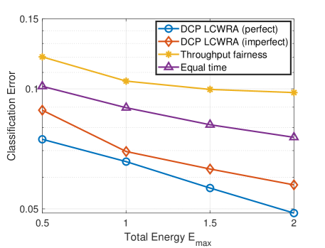
Based on the above settings, the classification error (i.e., the larger classification error between CNN and SVM) versus the total energy budget $E_{\rm{max}}=(0.5,1.0,1.5,2.0)$ in Joule at $T_{\rm{max}}=50~{}\rm{s}$ is shown in Fig. 2a. The maximum transmit power is set to $P_{\rm{max}}=(0.03,0.06,0.09,0.12)$ in Watt. Both perfect (i.e., $\{a_{m},b_{m}\}$ involve no estimation error) and imperfect (i.e., $\{a_{m},b_{m}\}$ involve $10\%$ estimation error) DCP-based LCWRA schemes are simulated. Besides the proposed DCP-based LCWRA algorithm, two benchmark schemes are also simulated: 1) the throughput fairness scheme [7]; 2) the time fairness scheme. It can be seen that no matter the parameters $\{a_{m},b_{m}\}$ are perfectly estimated or not, the proposed DCP-based LCWRA algorithm always achieves the minimum classification error and the error reduction could be up to $50\%$. This is because the proposed LCWRA finds that CNN is more difficult to train than SVM, and hence allocates more resources to user $1$. The proposed LCWRA collects $1253$ MNIST image samples, while the throughput fairness and time fairness schemes only collect $399$ and $553$ samples, respectively (when $(T_{\rm{max}},E_{\rm{max}},P_{\rm{max}})=(50,1,0.06)$). To verify the performance of the proposed ranking-based LCWRA, we consider the case of $E_{\rm{max}}=10$ and $P_{\rm{max}}=0.03$, and the classification error versus the total time budget $T_{\rm{max}}=(25,50,75,100)$ in second is shown in Fig. 2b. It can be seen from Fig. 2b that the proposed ranking-based LCWRA reduces the classification error by at least $20\%$.

Figure 2: Classification versus a) total energy at $T_{\rm{max}}=50~{}\rm{s}$ and $P_{\rm{max}}=(0.03,0.06,0.09,0.12)~{}\rm{W}$; b) total time at $E_{\rm{max}}=100~{}\rm{J}$ and $P_{\rm{max}}=0.03~{}\rm{W}$;

Finally, to demonstrate the effect of the number of nodes in the IoT application, we simulate 1) the case of $K=4$ with $\mathcal{Y}_{1}=\{1\}$ and $\mathcal{Y}_{2}=\{2,3,4\}$, and 2) the case of $K=6$ with $\mathcal{Y}_{1}=\{1,5,6\}$ and $\mathcal{Y}_{2}=\{2,3,4\}$. The worse error rate of the two tasks is 4.62% for the case of $K=6$ and 5.23% for the case of $K=4$. This indicates that more IoT nodes will improve the performance of the system. This is because more IoT nodes can generate more sensing data of various environment, and the edge could obtain a better training dataset by allocating resources to the new users $\{5,6\}$.

VI Experimental Results

TABLE I: Experimental Results

Scheme	Task	Communication				Learning
Name	Name	Time (s)	Rate (sample/s)	Total Numbr of Samples	Number of Samples	Online Accuracy	Minimum Online Accuracy	Offline Accuracy	Minimum Offline Accuracy
Time Fairness	CNN	$30$	$5$	450	140	65.3	65.3	75.5	75.5
	SVM	$30$	$10$		410	94.97		94.97
LCWRA	CNN	$48$	$5$	360 $(-20\%)$	210	74.5	74.5 $(+9.2\%)$	81.1	81.1 $(+5.6\%)$
	SVM	$12$	$10$		230	85.5		85.5

Due to the transmission overhead of control signals (which lead to reduced number of useful data) and random nature of wireless channels (e.g., disconnection/reconnection procedures), there is a mismatch between the simulated environment and the real-word environment. Therefore, in this section, two experiments to analyze the robustness of our scheme against practical uncertainties and complex environment are elaborated.

VI-A Robotic Image Dataset Collection

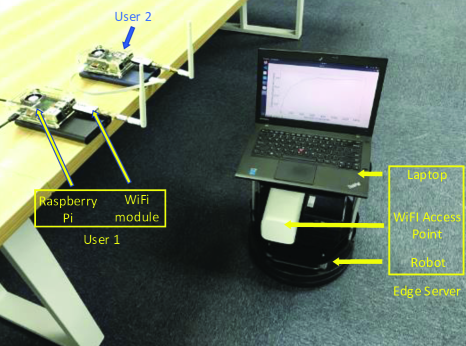
As shown in Fig. 3a, our first experiment consists of an mobile edge server and two IoT users. The edge server consists of a mobile robot (Turtlebot), a robot motion controller (Intel NUC), a computer (ThinkPad laptop), and a WiFi access point (Huawei 5G CPE Pro). The IoT user consists of a data storage module (Raspberry Pi 3 Model B) and a WiFi transmitter (with a $60~{}\rm{dB}$ attenuator to simulate the low transmit power of IoT devices). There are $1000$ MNIST data samples for training CNN and $1000$ digit samples for training SVM at user 1 and user 2 respectively.

All the functions are implemented using Python on a Ubuntu operating system. The communication between the edge and the IoT users is established using the IP address and the socket framework. A model training function (implemented based on Tensorflow), a data collection function (which tries to receive the wireless packets) and a buffer control function (which stores the collected data in a queue and updates the data batch before each training iteration) are developed at the edge server. A data transmission function (which tries to send the wireless packets) and a connection/reconnection function (which periodically searches for the target edge) are developed at each user.

In our experiment, the ranking-based scheme is implemented, which allocates the communication time according to Theorem 2. The total communication time is set to $1$ minute. The data-rates at users are fixed to $R_{1}=5D_{1}~{}\rm{bps}$ and $R_{2}=10D_{2}~{}\rm{bps}$ (i.e., user $1$ transmits $5$ samples per second and user $2$ transmits $10$ samples per second). The experiment is conducted in an office building shown in Fig. 3b, where user 1 is placed in the conference room and user 2 is placed in the corridor. The edge server has no historical data (i.e., $c_{1}=c_{2}=0$) and it cannot connect to both users at the initial location. As a result, the robot needs to move according to the trajectory defined in the ROS of Intel NUC, and communicate with different users at different locations. In our experiment, the server first enters the conference room to collect MNIST samples from user $1$, and then enters the corridor to collect digit samples from user $2$. Based on the above setup, the experimental results are shown in Table I. Compared with the time fairness scheme, the proposed LCWRA scheme improves the online accuracy (i.e., we test the trained models immediately after data collection) and the offline accuracy (we train the learning models until convergence and then test the models) by $9.2\%$ and $5.6\%$, respectively. The experiment demonstrates that the proposed LCWRA is robust against the uncertainty factors in real environment.

VI-B Vehicular Point-Cloud Dataset Collection

Figure 3: a) Experimental setup of the edge computing system; b) the edge data collection and training procedure.

Figure 4: Object detection results: a) task 1 with the LCWRA scheme; b) task 1 with the equal time allocation scheme; c) task 2 with the LCWRA scheme; d) task 2 with the equal time allocation scheme.

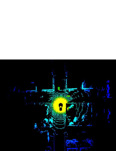
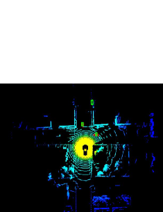
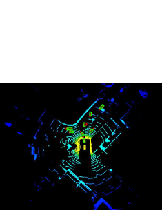
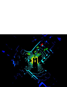
To verify the proposed LCWRA scheme in a more complex environment, we consider the use case of vehicular point-cloud dataset collection in Section II. Specifically, the case of $K=2$ with two different traffic scenarios is simulated: 1) sparse traffic scenario, and 2) dense traffic scenario. In each scenario, an autonomous driving car senses the environment, and generates on-board LiDAR point clouds. The sensing data is then uploaded to a network edge for model training. It is assumed that the transmission rates (controlled by the edge) at vehicles are fixed to $R_{1}=R_{2}=10~{}$samples/s. The total transmission time is $T_{\mathrm{max}}=16~{}$s. Notice that due to different traffics and environments, the learning error models for the two scenarios are different.

To simulate the two scenarios mentioned above, we employ the CARLA platform [29] for dataset generation and the SECOND neural network [19, 20] for object detection. Specifically, CARLA is an open-source simulator that supports development, training, and validation of autonomous driving systems. On the other hand, SECOND net is a voxel-based neural network that converts a point cloud to voxel features, and feeds the voxels into feature extraction and region proposal networks. As CARLA and SECOND are not compatible, we develop a data transformation module, such that the transformed dataset satisfies the KITTI standard [21].

Based on the above platform, we train the SECOND network for 50 epochs with a learning rate between $10^{-4}$ and $10^{-6}$ under different number of samples. Following similar procedures in Section V, the parameters in the error models for task 1 and task 2 are given by (3.95, 0.5) and (3.11, 0.71), respectively. Then, by executing our proposed algorithms, the numbers of collected data samples for the two tasks are obtained as 137 and 22. In contrast, with the equal-time allocation scheme, $80$ samples are collected for both task 1 and task 2. The trained models are tested on two validation datasets, each with 193 unseen samples ($>1000$ objects). The worse learning accuracies of the two tasks are $67.3\%$ for LCWRA algorithm and $46.84\%$ for equal time scheme, respectively. It can be seen from the Fig. 4 that by using the LCWRA algorithm, the performance of task 1 is significantly improved while the performance of task 2 is still acceptable.

VII Conclusions

This paper introduced the LCWRA scheme for edge intelligence systems. The joint energy and time allocation scheme was derived based on DCP and the asymptotic solution proved the inverse power relationship between the generalization error and the transmission time. Simulation results showed that the proposed LCWRA scheme significantly outperforms existing resource allocation schemes. Experiments demonstrated the robustness of the proposed algorithm in practical and complex environment.

Appendix A Proof of Theorem 2

First, if $\left(u^{\diamond}/a_{m}\right)^{-\frac{1}{b_{m}}}-c_{m}\leq 0$, the first constraint of P3[m] is always satisfied and P3[m] is equivalently written as

$$\min_{\{z_{i,m}\}}\quad \sum_{i=1}^{|\mathcal{Y}_{m}|}z_{i,m},$$

s.t. $$U_{i,m}z_{i,m}\leq V_{i,m},\quad i=1,...,|\mathcal{Y}_{m}|,$$ (15a)

$$z_{i,m}\geq 0,\quad i=1,...,|\mathcal{Y}_{m}|.$$ (15b)

It is clear that the optimal solution to the above problem is $z_{i,m}^{*}=0$.

On the other hand, if $\left(u^{\diamond}/a_{m}\right)^{-\frac{1}{b_{m}}}-c_{m}>0$, the Lagrangian of P3[m] is given by

$$L =\sum_{i=1}^{|\mathcal{Y}_{m}|}z_{i,m}+\lambda_{m}\left(\left(\frac{u^{\diamond}}{a_{m}}\right)^{-\frac{1}{b_{m}}}-c_{m}-\sum_{i=1}^{|\mathcal{Y}_{m}|}U_{i,m}\,z_{i,m}\right)$$

$$\quad{}{}+\sum_{i=1}^{|\mathcal{Y}_{m}|}\beta_{i,m}\left(U_{i,m}\,z_{i,m}-V_{i,m}\right)-\sum_{i=1}^{|\mathcal{Y}_{m}|}\gamma_{i,m}z_{i,m},$$ (16)

where $\left\{\lambda_{m},\beta_{i,m},\gamma_{i,m}\right\}$ are non-negative Lagrangian multipliers. According to KKT conditions, the following equations hold:

$$\frac{\partial L}{\partial z^{*}_{i,m}}=1-U_{i,m}\lambda_{m}+U_{i,m}\beta_{i,m}-\gamma_{i,m} =0,\quad\forall i,$$ (17a)

$$\lambda_{m}\left(\left(\frac{u^{\diamond}}{a_{m}}\right)^{-\frac{1}{b_{m}}}-c_{m}-\sum_{i=1}^{|\mathcal{Y}_{m}|}U_{i,m}\,z_{i,m}\right) =0,$$ (17b)

$$\beta_{i,m}\left(U_{i,m}\,z_{i,m}-V_{i,m}\right) =0,\quad\forall i,$$ (17c)

$$\gamma_{i,m}z_{i,m} =0,\quad\forall i.$$ (17d)

$$\left(\frac{u^{\diamond}}{a_{m}}\right)^{-\frac{1}{b_{m}}}-c_{m}-\sum_{i=1}^{|\mathcal{Y}_{m}|}U_{i,m}\,z_{i,m} \leq 0,\quad\forall i$$ (17e)

$$U_{i,m}\,z_{i,m}-V_{i,m} \leq 0,\quad\forall i,$$ (17f)

$$z_{i,m} \geq 0,\quad\forall i.$$ (17g)

Based on (17a)–(17g), we will first prove $\gamma_{1,m}=0$ by contradiction. Suppose that $\gamma_{1,m}\neq 0$. From (17d), we obtain $z^{*}_{1,m}=0$. As $\left(u^{\diamond}/a_{m}\right)^{-\frac{1}{b_{m}}}-c_{m}>0$, and according to (17e), we must have $\sum_{i=1}^{|\mathcal{Y}_{m}|}U_{i,m}\,z_{i,m}>0$. This means that there exists some $j$ such that $z^{*}_{j,m}>0$. Now, consider another solution $\{z_{i,m}^{\prime}\}$:

$$z_{i,m}^{\prime}=\begin{cases}\frac{\Delta}{U_{1,m}}&i=1\\ z^{*}_{j,m}-\frac{\Delta}{U_{j,m}}&i=j\\ z^{*}_{i,m}&i\notin\left\{1,j\right\}\end{cases},$$ (18)

where $\Delta>0$ is a small constant. Since 1) $\sum_{i}U_{i,m}z^{*}_{i,m}=\sum_{i}U_{i,m}z_{i,m}^{\prime}$; 2) $\frac{\Delta}{U_{1,m}}\leq V_{i,m}$; and 3) $z_{i,m}^{\prime}\geq 0$, $\{z_{i,m}^{\prime}\}$ is a feasible solution to P3[m]. However, the objective $\sum_{i}z_{i,m}^{\prime}=\sum_{i}z_{i,m}^{*}+\frac{\Delta}{U_{1,m}}-\frac{\Delta}{U_{j,m}}<\sum_{i}z_{i,m}^{*}$, where the inequality is due to $U_{1,m}>U_{j,m}$. This contradicts to $\{z^{*}_{i,m}\}$ being optimal.

Next, putting $\gamma_{1,m}=0$ into (17a), we have

$$U_{1,m}\lambda_{m}=1+U_{1,m}\beta_{1,m}.$$ (19)

Since $U_{1,m}\beta_{1,m}\geq 0$, we have $\lambda_{m}>0$. According (17b), the following equation holds:

$$\sum_{i=1}^{|\mathcal{Y}_{m}|}U_{i,m}z^{*}_{i,m}=\left(\frac{u^{\diamond}}{a_{m}}\right)^{-\frac{1}{b_{m}}}-c_{m}.$$ (20)

To derive $z^{*}_{i,m}$, we consider two cases.

• If $\beta_{1,m}\neq 0$, then $z^{*}_{1,m}=\frac{V_{1,m}}{U_{1,m}}$ according to (17c). In this case, $z^{*}_{1,m}\leq\frac{1}{U_{1,m}}\left(u^{\diamond}/a_{m}\right)^{-\frac{1}{b_{m}}}-\frac{c_{m}}{U_{1,m}}$ (which is obtained by putting $z^{*}_{1,m}=\frac{V_{1,m}}{U_{1,m}}$ into (20)).

• If $\beta_{1,m}=0$, then $\lambda_{m}=\frac{1}{U_{1,m}}$ according to (19). Putting this result into (17a), we have $1-\frac{U_{i,m}}{U_{1,m}}+U_{i,m}\beta_{i,m}-\gamma_{i,m}=0$. But since $U_{1,m}>U_{i,m}>0$ for any $i>1$ and $\beta_{i,m}\geq 0$, we obtain $\gamma_{i,m}>0$, meaning that $z^{*}_{i,m}=0$ for any $i>1$. Further due to (20), we have $z^{*}_{1,m}=\frac{1}{U_{1,m}}\left(u^{\diamond}/a_{m}\right)^{-\frac{1}{b_{m}}}-\frac{c_{m}}{U_{1,m}}$. In this case, $z^{*}_{1,m}\leq\frac{V_{1,m}}{U_{1,m}}$ (which is obtained from (17f)).

Based on the above discussions, $z^{*}_{1,m}$ is given by

$$z^{*}_{1,m}=\min\left\{\frac{V_{1,m}}{U_{1,m}},\,\frac{1}{U_{1,m}}\left(\frac{u^{\diamond}}{a_{m}}\right)^{-\frac{1}{b_{m}}}-\frac{c_{m}}{U_{1,m}}\right\}.$$ (21)

With the optimal $z^{*}_{1,m}$, the optimal $z^{*}_{j,m}$ with $j>1$ can be obtained by induction. More specifically, assuming that the optimal $z^{*}_{1,m},\cdots,z^{*}_{j-1,m}$ is known at the $j$-th iteration, and defining $S_{j,m}=\left(u^{\diamond}/a_{m}\right)^{-\frac{1}{b_{m}}}-c_{m}-\sum_{i=1}^{j-1}U_{i,m}z_{i,m}^{*}$, problem P3[m] is equivalently written into

$$\min_{\{z_{i,m}\}}\quad \sum_{i=j}^{|\mathcal{Y}_{m}|}z_{i,m},$$

s.t. $$\sum_{i=j}^{|\mathcal{Y}_{m}|}U_{i,m}z_{i,m}\geq S_{j,m},$$ (22a)

$$U_{i,m}z_{i,m}\leq V_{i,m},\quad i=j,...,|\mathcal{Y}_{m}|,$$ (22b)

$$z_{i,m}\geq 0,\quad i=j,...,|\mathcal{Y}_{m}|.$$ (22c)

It can be seen that the above problem has the same form as $\mathrm{P}3[m]$. Furthermore, $U_{j,m}$ is the largest among $\{U_{j,m},\cdots,U_{|\mathcal{Y}_{m}|,m}\}$. Therefore, the optimal $z^{*}_{j,m}$ can be obtained following a similar derivation in (21) and the proof is completed.

References

- [1] Y. Mao, C. You, J. Zhang, K. Huang, and K. B. Letaief, “A survey on mobile edge computing: The communication perspective,” IEEE Commun. Surv. Tutor., vol. 19, no. 4, pp. 2322–2358, Fourthquarter 2017.
- [2] S. Yu, X. Chen, L. Yang, D. Wu, M. Bennis, and J. Zhang, “Intelligent edge: Leveraging deep imitation learning for mobile edge computation offloading,” IEEE Wireless Commun., vol. 27, no. 1, pp. 92–99, Feb. 2020.
- [3] Z. Zhou, X. Chen, E. Li, L. Zeng, K. Luo, and J. Zhang, “Edge intelligence: Paving the last mile of artificial intelligence with edge computing,” Proc. IEEE, vol. 107, no. 8, pp. 1738–1762, Aug. 2019.
- [4] S. Wang, Y.-C. Wu, M. Xia, R. Wang, and H. V. Poor, “Machine intelligence at the edge with learning centric power allocation,” vol. 19, no. 11, pp. 7293–7308, Jul. 2020.
- [5] S. Wang, R. Wang, Q. Hao, Y.-C. Wu, and H. V. Poor, “Learning centric power allocation for edge intelligence,” in Proc. IEEE ICC, Dublin, Ireland, Jun. 2020.
- [6] G. Zhu, Y. Wang, and K. Huang, “Broadband analog aggregation for low-latency federated edge learning,” IEEE Trans. Wireless Commun., vol. 19, no. 1, pp. 491–506, Jan. 2020.
- [7] L. Li, M. Pal and Y. R. Yang, “Proportional fairness in multi-rate wireless LANs,” IEEE INFOCOM 2008, Phoenix, AZ, 2008, pp. 1004–1012.
- [8] M. Chen, S. Wang, S. Liao, I. Chung, and C. Chou, “Deadline is not enough: Importance-aware transmission control protocol for server-centric data centers,” IEEE Syst. J., vol. 12, no. 2, pp. 1543–1553, Jun. 2018.
- [9] G. Zhu, D. Liu, Y. Du, C. You, J. Zhang, and K. Huang, “Toward an intelligent edge: Wireless communication meets machine learning,” IEEE Commun. Mag., vol. 58, no. 1, pp. 19–25, Jan. 2020.
- [10] 3GPP, “5G; NR; Physical layer procedures for control,” TS 38.213 version 15.5.0 Release 15, May 2019.
- [11] M. Chen, Z. Yang, W. Saad, C. Yin, H. V. Poor, and S. Cui, “A joint learning and communications framework for federated learning over wireless networks,” IEEE Trans. Wireless Commun., 2020. DOI: 10.1109/TWC.2020.3024629.
- [12] T. Domhan, J. T. Springenberg, F. Hutter, “Speeding up automatic hyperparameter optimization of deep neural networks by extrapolation of learning curves,” in Proc. IJCAI, Buenos Aires, Argentina, Jul. 2015.
- [13] M. Johnson, P. Anderson, M. Dras, and M. Steedman, “Predicting classification error on large datasets from smaller pilot data,” in Proc. ACL, Melbourne, Australia, Jul. 2018, pp. 450–455.
- [14] H. S. Seung, H. Sompolinsky, and N. Tishby, “Statistical mechanics of learning from examples,” Phys. Rev. A, vol. 45, pp. 6056–6091, Apr. 1992.
- [15] S. C. Ergen and P. Varaiya, “TDMA scheduling algorithms for wireless sensor networks,” Wireless Netw., vol. 16, no. 4, pp. 985–997, May 2010.
- [16] S. Zafar, S. Jangsher, M. Aloqaily, O. Bouachir, and J. B. Othman, “Resource allocation in moving small cell network using deep learning-based interference determination,” in Proc. IEEE PIMRC, Sept. 2019.
- [17] H. F. Saeeda, S. Jangsher, M. Aloqaily, H. K. Qureshi, and J. BenOthman, “Joint pairing and resource allocation for backhaul of small cells using NOMA,” Journal of Computational Science, vol. 45, Sep. 2020.
- [18] V. Balasubramanian, F. Zaman, M. Aloqaily, S. Alrabaee, M. Gorlatova, and M. Reisslein, “Reinforcing the edge: Autonomous energy management for mobile device clouds,” in Proc. IEEE INFOCOM WKSHPS, Apr.–May 2019, pp. 44–49.
- [19] Y. Yan, Y. Mao, and B. Li, “SECOND: Sparsely embedded convolutional detection,” Sensors, vol. 18, no. 10, pp. 3337, Oct. 2018.
- [20] S. Shi, Z. Wang, J. Shi, X. Wang, and H. Li, “From points to parts: 3D object detection from point cloud with part-aware and part-aggregation network,” IEEE Trans. Pattern Anal. Mach. Intell., 2020. DOI: 10.1109/TPAMI.2020.2977026.
- [21] A. Geiger, P. Lenz, C. Stiller, and R. Urtasun, “Vision meets robotics: The kitti dataset,” International Journal of Robotics Research, vol. 32, pp. 1231–1237, Aug. 2013.
- [22] S. Boyd and L. Vandenberghe, Convex Optimization. Cambridge, U.K.: Cambridge Univ. Press, 2004.
- [23] Y. Sun, P. Babu, and D. P. Palomar, “Majorization-minimization algorithms in signal processing, communications, and machine learning,” IEEE Trans. Signal Process., vol. 65, no. 3, pp. 794–816, Feb. 2017.
- [24] L. Zhou, Y. Hong, S. Wang, R. Han, D. Li, R. Wang, and Q. Hao, “Learning centric wireless resource allocation for edge computing: Algorithm and experiment,” [Online]. Available: https://arxiv.org/pdf/2010.15371.pdf, 2020.
- [25] L. Deng, “The MNIST database of handwritten digit images for machine learning research,” IEEE Signal Process. Mag., vol. 29, no. 6, pp. 141–142, Nov. 2012.
- [26] F. Pedregosa, G. Varoquaux, A. Gramfort, et al., “Scikit-learn: Machine learning in Python,” J. Mach. Learn. Res., vol. 12, pp. 2825–2830, Oct. 2011.
- [27] H. Q. Ngo, E. G. Larsson, and T. L. Marzetta, “Energy and spectral efficiency of very large multiuser MIMO systems,” IEEE Trans. Commun., vol. 61, no. 4, pp. 1436–1449, Apr. 2013.
- [28] 3GPP, “Performance requirements for Narrowband IoT,” TS 36.104 version 15.3.0 Release 15, Jul. 2018.
- [29] A. Dosovitskiy, G. Ros, F. Codevilla, A. Lopez, and V. Koltun, “CARLA: An open urban driving simulator,” in Proc. The 1st Annual Conference on Robot Learning, 2017, pp. 1–16.