An Evaluation of The Proton Structure Functions $F_{2}$ and $F_{L}$ at Small $x$

Abstract

We describe the determination of the DIS structure functions $F_{2}$ and $F_{L}$ by using the singlet Dokshitzer-Gribov-Lipatov-Altarelli-Parisi (DGLAP) and Altarelli-Martinelli equations at small values of $x$. The determination of the longitudinal structure function is presented as a parameterization of $F_{2}(x,Q^{2})$ and its derivative. Analytical expressions for $\sigma_{r}(x,Q^{2})$ in terms of the effective parameters of the parameterization of $F_{2}(x,Q^{2})$ and $F_{L}(x,Q^{2})$ are presented. This analysis is enriched by including the higher-twist effects in calculation of the reduced cross sections which is important at low-$x$ and low-$Q^{2}$ regions. Numerical calculations and comparison with H1 data demonstrate that the suggested method provides reliable $F_{L}(x,Q^{2})$ and $\sigma_{r}(x,Q^{2})$ at low $x$ in a wide range of the low absolute four-momentum transfers squared ($1.5~{}\mathrm{GeV}^{2}<Q^{2}<120~{}\mathrm{GeV}^{2}$) at moderate and high inelasticity. Expanding the method to low and ultra low values of $x$ can be considered in the process analysis of new colliders. We compare the obtained longitudinal structure function with respect to the LHeC simulated uncertainties [CERN-ACC-Note-2020-0002, arXiv:2007.14491 [hep-ex] (2020)] with the results from CT18 [Phys.Rev.D103, 014013(2021)] parametrization model.

.1 I. INTRODUCTION

The experimental determination of the longitudinal structure function is a realistic prospect at high energy electron-proton colliders. First measurements of $F_{L}$ at small $x$ were performed at HERA [1]. A next generation of ep colliders is under design, the Large Hadron electron Collider (LHeC) [2,3] and the Future Circular Collider electron- hadron (FCC-eh) [4] where these measurements can be performed with much increased precision and extended to much lower values of $x$ and high $Q^{2}$. The electron-proton center-of-mass energy at the LHeC can reach to $\sqrt{s}\simeq 1.3~{}\mathrm{TeV}$, which this is about 4 times the center-of-mass energy range of ep collisions at HERA [2,3]. The LHeC is designed to become the finest new microscope for exploring new physics, as the kinematic range in the ($x,Q^{2}$) plane for electron and positron neutral-current (NC) in the perturbative region is well below $x{\approx}10^{-6}$ and extends up to $Q{\simeq}1~{}\mathrm{TeV}$. HERA has also reached to $x{\sim}10^{-6}$ in $Q^{2}$ values $0.2$, $0.11$ and $0.045~{}\mathrm{GeV}^{2}$ which is related to the H1 svx-mb, ZEUS BPC and ZEUS BPT data sets respectively [4]. This behavior will be extended down to $x\simeq 10^{-7}$ at the FCC-eh option of a Future Circular Collider program [5]. The FCC-eh collider would reach a center-of-mass energy of $\sqrt{s}=3.5~{}\mathrm{TeV}$ at a similar luminosity as the LHeC. Deep inelastic scattering measurements at the FCC-eh and the LHeC will allow the determination of parton distribution functions at very small $x$ as they are pertinent in investigations of lepton-hadron processes in ultra-high energy (UHE) neutrino astroparticle physics [5]. Moreover a similar very high energy electron-proton/ion collider (VHEep) [6] has been suggested based on plasma wakefield acceleration, albeit with very low luminosity. The center-of-mass energy, in this collider, is close to $10~{}\mathrm{TeV}$ which is relevant in investigations of new strong interaction dynamics related to high-energy cosmic rays and gravitational physics (the luminosity estimate is about six orders of magnitude below that of LHeC).
Recently several methods for the determination of the longitudinal structure function in the nucleon from the proton structure function have been proposed [7-11]. The method is based on a form of the deep inelastic lepton-hadron scattering (DIS) structure function which was proposed by Block-Durand-Ha (BDH) in Ref.[12]. This new parameterization describes accurately the results for the high energy ep and isoscalar ${\nu}N$ total cross sections. These cross sections obey an analytic expression as a function of ${\mathrm{\ln}}\mathrm{E}$ at large energies $\mathrm{E}$ of the incident particle. Indeed, this parameterization is relevant for investigations of ultra-high energy processes, such as scattering of cosmic neutrinos from hadrons [7].
At low values of $x$, the transversal structure function $F_{2}(x,Q^{2})$ and the longitudinal structure function $F_{L}(x,Q^{2})$ are defined solely via the singlet quark $xf_{s}(x,Q^{2})$ and gluon density $xf_{g}(x,Q^{2})$ as

$$F_{k}(x,Q^{2})=<e^{2}>\sum_{a=s,g}\bigg{[}B_{k,a}(x){\otimes}xf_{a}(x,Q^{2})\bigg{]},~{}~{}~{}k=2,L$$

where $<e^{2}>=\frac{\sum_{i=1}^{N_{f}}e_{i}^{2}}{N_{f}}$ is the average charge squared for ${N_{f}}$ which ${N_{f}}$ denotes the number of effective massless flavours. The quantities $B_{k,a}(x)$ are the known Wilson coefficient functions and the parton densities fulfil the renormalization group evolution equations. Here the non-singlet densities become negligibly small in comparison with the singlet densities. The symbol $\otimes$ indicates convolution over the variable $x$ by the usual form, $f(x){\otimes}g(x)=\int_{x}^{1}\frac{dz}{z}f(z,\alpha_{s})g(x/z)$. It is important to resum the leading $\alpha_{s}\log(1/x)$ contributions at low values of $x$, where this resummation is accomplished by the BFKL equation [13]. In this region, the gluon density is predicted to increase as this singular behavior of growth in $x$ is the characteristic property of the BFKL gluon density.
Some time ago a proposal was published to look for the longitudinal and transversal structure functions in deep inelastic scattering (DIS) [14]. The authors in Ref.[14] showed that it is possible to obtain scheme independent evolution equations for the structure functions by the following form

$$\frac{{\partial}F_{2}(x,Q^{2})}{{\partial}{\ln}Q^{2}}\sim\Gamma_{22}\otimes F_{2}(x,Q^{2})+\Gamma_{2L}\otimes F_{L}(x,Q^{2}),$$ (1)

$$\frac{{\partial}F_{L}(x,Q^{2})}{{\partial}{\ln}Q^{2}}\sim\Gamma_{L2}\otimes F_{2}(x,Q^{2})+\Gamma_{LL}\otimes F_{L}(x,Q^{2}).$$ (2)

The method is based on physical observables, $F_{L}$ and $F_{2}$. The anomalous dimensions $\Gamma_{ij}$ are computable in perturbative QCD. The structure functions $F_{2}$ and $F_{L}$ are related to the cross sections $\sigma_{T}$ and $\sigma_{L}$ for interaction of transversely and longitudinally polarised photons with protons. The reduced cross section for deep-inelastic lepton-proton scattering depends on these independent structure functions in the combination

$${\sigma}(x,Q^{2})=F_{2}(x,Q^{2})-\frac{y^{2}}{Y_{+}}F_{L}(x,Q^{2}),$$ (3)

where $Y_{+}=1+(1-y)^{2}$, $y={Q^{2}}/{xs}$ denotes the inelasticity and $s$ stands for the center-of-mass energy squared of incoming electrons and protons. As usual $x$ is the Bjorken scaling parameter and $Q^{2}$ is the four momentum transfer in a deep inelastic scattering process.
In QCD, structure functions are defined as convolution of universal parton momentum distributions inside the proton and coefficient functions, which contain information about the boson-parton interaction [15,16]. The standard and the basic tools for theoretical investigation of DIS structure functions are the DGLAP evolution equations [17,18]. The DGLAP equations based on the parton model and perturbative QCD theory successfully and quantitatively interpret the $Q^{2}$-dependence of parton distribution functions (PDFs). It is so successful that most of the PDFs are extracted by using the DGLAP equations up to now. These equations can be used to extract the deep inelastic scattering structure functions of proton.
The longitudinal structure function $F_{L}(x,Q^{2})$ of the proton in terms of coefficient function is given by [17]

$$x^{-1}F_{L}(x,Q^{2}) = C_{L,ns}(\alpha_{s},x){\otimes}q_{ns}(x,Q^{2})$$ (4)

$$+<e^{2}>[C_{L,s}(\alpha_{s},x){\otimes}q_{s}(x,Q^{2})$$

$$+C_{L,g}(\alpha_{s},x){\otimes}g(x,Q^{2})],$$

where $q_{ns}$, $q_{s}$ and $g$ are the flavour non singlet, flavour singlet and gluon density respectively. The coefficient functions $C_{L,a}(a=q,g)$ can be written in a perturbative expansion as follows [19]:

$$C_{L,a}(\alpha_{s},x)=\sum_{n=1}(\frac{\alpha_{s}}{4\pi})^{n}c^{(n)}_{L,a}(x),$$

where $n$ denotes the order in running coupling. The coupled DGLAP evolution equations for the singlet quark structure function $F_{s}(x,Q^{2})=\sum_{i}x[q_{i}(x,Q^{2})+\overline{q}_{i}(x,Q^{2})]$ and the gluon distribution $G(x,Q^{2})=xg(x,Q^{2})$ can be written as

$$\frac{{\partial}G(x,Q^{2})}{{\partial}{\ln}Q^{2}} = P_{gg}(\alpha_{s},x){\otimes}G(x,Q^{2})$$ (5)

$$+P_{gq}(\alpha_{s},x){\otimes}F_{s}(x,Q^{2}),$$

$$\frac{{\partial}F_{s}(x,Q^{2})}{{\partial}{\ln}Q^{2}} = P_{qq}(\alpha_{s},x){\otimes}F_{s}(x,Q^{2})$$ (6)

$$+2N_{f}P_{qg}(\alpha_{s},x){\otimes}G(x,Q^{2}).$$

The splitting functions $P_{ij}$ are the Altarelli-Parisi kernels at LO up to high-order corrections [20]

$$P_{ij}(\alpha_{s},x)=\sum_{n=1}(\frac{\alpha_{s}}{4\pi})^{n}P^{(n)}_{ij}(x),$$

where $\alpha_{s}(Q^{2})$ is the running coupling.
The main purpose of the article is to study the relationship between the structure functions, which is expected to be more reliable at small $x$. Indeed, with respect to the DGLAP evolution equations, the direct relationship between the longitudinal structure function and the proton structure function is examined. Then the effects of Higher-twist (HT) on the reduced cross sections at low-$Q^{2}$ values are considered. The organization of this paper is as follows. In section II we introduce the basic formula used for the definition of decoupling DGLAP evolution equations into the proton and longitudinal structure functions. In section III we present the longitudinal structure function with respect to the parameterization of $F_{2}$. In section IV we also present the effective exponent for the singlet structure function in an independent method. Finally the formalism of HT effects used in this analysis in section V is described. The main results and finding of the present longitudinal structure function and reduced cross section at moderate and high inelasticity are discussed in detail in section VI. In the same section, we present the extracted HT effects at low $Q^{2}$ values and show detailed comparisons with the experimental data. We also expand the available energy to the range of new collider energies (i.e., LHeC and FCC-eh). This section also includes a brief discussion of the implication of the finding for future research. Conclusions and summary are summarized on Sec.VII.

.2 II. BASIC FORMULA

The standard parameterization of the singlet and gluon distribution functions for $x{\rightarrow}0$, is given by [21,22]

$$F_{2}^{s}(x,Q^{2})_{x{\rightarrow}0} = A_{s}(Q^{2})x^{-\lambda_{s}(Q^{2})},$$

$$G(x,Q^{2})_{x{\rightarrow}0} = A_{g}(Q^{2})x^{-\lambda_{g}(Q^{2})},$$ (7)

where $A_{s}$ and $A_{g}$ are $Q^{2}$ dependent and $\lambda^{,}$s are strictly positive. This behavior of the singlet structure function was proposed by Lopez and Yndurain [21], and the inclusive electroproduction on a proton was studied at low $x$ and low $Q^{2}$ using a soft and hard Pomeron in Ref.[22]. The gluon exponent at low values of $x$ at $Q^{2}=1~{}\mathrm{GeV}^{2}$ obtained by MSTW08 NLO was $0.428^{+0.066}_{-0.057}$ [23]. The effective exponent for the gluon distribution at $Q^{2}=10~{}\mathrm{GeV}^{2}$ and $x=10^{-4}$ obtained by NNPDF3.0, CT14, MMHT14, ABM12 and CJ15 had values of 0.20, 0.15, 0.29, 0.15 and 0.14 respectively. The value obtained by fixed coupling LLx BFKL gives $\lambda_{g}{\simeq}0.5$, which is the so-called hard-Pomeron exponent. Some other phenomenological models have also been proposed for the singlet structure function exponents in Refs.[24] and [25]. The singlet and gluon exponents are determined and applied to the deep inelastic lepton nucleon scattering at low values of $x$ in Ref.[26]. Ref.[27] used a form inspired by double asymptotic $x,Q^{2}$ scaling. The hard Pomeron behavior of the photon-proton cross section based on a simple power-law behavior and double asymptotic scaling at low $x$ values for $10<W<10^{4}~{}\mathrm{GeV}$ in the kinematic range of VHEep is shown in Ref.[6]. Recently, authors in Ref.[28] presented a tensor-Pomeron model where it is applied to low-$x$ deep inelastic lepton-nucleon scattering and photoproduction processes. In this model, in addition to the soft tensor Pomeron, a hard tensor Pomeron and Reggeon exchange included. In this case the hard-Pomeron intercept was determined to $0.3008(^{+73}_{-84})$ with the latest HERA data for $x<0.01$. An effective behavior for the singlet structure function is reported in Refs.[24] and [29]. This effective exponent was found to be independent of $x$ and to increase linearly with ${\ln}Q^{2}$. Indeed the function $\lambda(Q^{2})$ was determined from fits of the form $F_{2}(x,Q^{2})=c(Q^{2})x^{-\lambda(Q^{2})}$ to the H1 data, and the coefficients $c(Q^{2})$ are approximately independent of $Q^{2}$ and $\lambda(Q^{2})$ rises linearly with ${\ln}Q^{2}$.
Now we use the hard pomeron behavior for the distribution functions (i.e., Eq.(7)) in Eqs.(4-6) and obtain the modified evolution equations, which take into account all the modifications mentioned above, by the following forms

$$\frac{{\partial}G(x,Q^{2})}{{\partial}{\ln}Q^{2}} = G(x,Q^{2})\Phi_{gg}(x,Q^{2})$$ (8)

$$+F_{2}(x,Q^{2})\Theta_{gq}(x,Q^{2}),$$

$$\frac{{\partial}F_{2}(x,Q^{2})}{{\partial}{\ln}Q^{2}} = F_{2}(x,Q^{2})\Phi_{qq}(x,Q^{2})$$ (9)

$$+G(x,Q^{2})\Theta_{qg}(x,Q^{2}),$$

and

$$F_{L}(x,Q^{2}) = F_{2}(x,Q^{2})I_{L,q}(x,Q^{2})$$ (10)

$$+G(x,Q^{2})I_{L,g}(x,Q^{2}).$$

The convolution and the compact form of the kernels are given by

$$\Phi_{qq}(x,Q^{2}) = P_{qq}(x,\alpha_{s}){\odot}x^{\lambda_{s}(Q^{2})}$$

$$\Phi_{gg}(x,Q^{2}) = ~{}P_{gg}(x,\alpha_{s}){\odot}x^{\lambda_{g}(Q^{2})}$$

$$\Theta_{gq}(x,Q^{2}) = \frac{18}{5}P_{gq}(x,\alpha_{s}){\odot}x^{\lambda_{s}(Q^{2})}$$

$$\Theta_{qg}(x,Q^{2}) = \frac{10N_{f}}{18}P_{qg}(x,\alpha_{s}){\odot}x^{\lambda_{g}(Q^{2})}$$

$$I_{L,q}(x,Q^{2}) = ~{}\frac{18}{5N_{f}}C_{L,q}(x,\alpha_{s}){\odot}x^{\lambda_{s}(Q^{2})}$$

$$I_{L,g}(x,Q^{2}) = <e^{2}>C_{L,g}(x,\alpha_{s}){\odot}x^{\lambda_{g}(Q^{2})},$$ (11)

where we have defined the convolution form to be

$$f(x){\odot}g(x)=\int_{x}^{1}\frac{dz}{z}f(\alpha_{s},z)g(z).$$ (12)

These equations (i.e., Eqs.(8-10)) can now be easily decoupled. The idea is to modify the evolution equations in order to satisfy simultaneously the decoupled evolution equation based on the structure functions. Indeed, in this method, we separate the gluon distribution function from Eqs.(8-10). In fact the singlet and longitudinal structure functions contain the gluon distribution which comes from the perturbative QCD. Therefore the solution of Eq.(10) is straightforward and given by

$$G(x,Q^{2})=\frac{F_{L}(x,Q^{2})}{I_{L,g}(x,Q^{2})}-F_{2}(x,Q^{2})\frac{I_{L,q}(x,Q^{2})}{I_{L,g}(x,Q^{2})}.$$ (13)

Using Eq.(13) in (9), our solution takes the form

$$\frac{{\partial}F_{2}(x,Q^{2})}{{\partial}{\ln}Q^{2}} = \Gamma_{22}(x,Q^{2})F_{2}(x,Q^{2})$$ (14)

$$+\Gamma_{2L}(x,Q^{2})F_{L}(x,Q^{2}),$$

where

$$\Gamma_{22}(x,Q^{2}) = \Phi_{qq}(x,Q^{2})-\Theta_{qg}(x,Q^{2})\frac{I_{L,q}(x,Q^{2})}{I_{L,g}(x,Q^{2})},$$

$$\Gamma_{2L}(x,Q^{2}) = \frac{\Theta_{qg}(x,Q^{2})}{I_{L,g}(x,Q^{2})}.$$ (15)

Also substituting Eq.(13) in Eq.(8) we get

$$\frac{{\partial}F_{L}(x,Q^{2})}{{\partial}{\ln}Q^{2}} = \Gamma_{LL}(x,Q^{2})F_{L}(x,Q^{2})$$ (16)

$$+\Gamma_{L2}(x,Q^{2})F_{2}(x,Q^{2}),$$

where

$$\Gamma_{LL}(x,Q^{2}) = T_{LL}(x,Q^{2})+\frac{{\partial}}{{\partial}{\ln}Q^{2}}{\ln}I_{L,g}(x,Q^{2}),$$

$$\Gamma_{L2}(x,Q^{2}) = T_{L2}(x,Q^{2})+I_{L,q}(x,Q^{2})$$ (17)

$${\times}\frac{{\partial}}{{\partial}{\ln}Q^{2}}{\ln}\frac{I_{L,q}(x,Q^{2})}{I_{L,g}(x,Q^{2})}.$$

and

$$T_{LL}(x,Q^{2}) = \Phi_{gg}(x,Q^{2})+\Theta_{qg}(x,Q^{2})\frac{I_{L,q}(x,Q^{2})}{I_{L,g}(x,Q^{2})},$$

$$T_{L2}(x,Q^{2}) = I_{L,q}(x,Q^{2})[\Phi_{qq}(x,Q^{2})-\Phi_{gg}(x,Q^{2})$$ (18)

$$-\Theta_{qg}(x,Q^{2})\frac{I_{L,q}(x,Q^{2})}{I_{L,g}(x,Q^{2})}]$$

$$+\Theta_{gq}(x,Q^{2})I_{L,g}(x,Q^{2}).$$

Therefore the evolution equations for the structure functions $F_{2}(x,Q^{2})$ and $F_{L}(x,Q^{2})$ read as

$$\frac{{\partial}}{{\partial}{\ln}Q^{2}}\left(\begin{array}[]{c}F_{2}(x,Q^{2})\\ F_{L}(x,Q^{2})\end{array}\right)=\left(\begin{array}[]{cc}\Gamma_{22}&\Gamma_{2L}\\ \Gamma_{L2}&\Gamma_{LL}\end{array}\right){\times}\left(\begin{array}[]{c}F_{2}(x,Q^{2})\\ F_{L}(x,Q^{2})\end{array}\right).$$ (25)

.3 III. DETERMINING THE LONGITUDINAL STRUCTURE FUNCTION

One can rewrite Eq.(13) related to the proton structure function $F_{2}(x,Q^{2})$ and its derivative with respect to ${\ln}Q^{2}$, as we have

$$F_{L}(x,Q^{2}) = \frac{1}{\Gamma_{2L}}\frac{{\partial}F_{2}(x,Q^{2})}{{\partial}{\ln}Q^{2}}-\frac{\Gamma_{22}}{\Gamma_{2L}}F_{2}(x,Q^{2}).$$ (27)

This relation (i.e., Eq.(20)) help to estimate the proton longitudinal structure function in terms of the effective parameters of the parametrization of $F_{2}(x,Q^{2})$. We now employ the $F_{2}$ parameterization of Ref.[12] which is obtained from a combined fit of the HERA data [4] with $x\leq 0.1$ and $W\geq 25~{}\mathrm{GeV}$ and use it in Eq.(20). This parametrization describes fairly good the available experimental data on the proton structure function in agreement with the Froissart [30] bound behavior. The explicit expression for the $F_{2}$ parametrization [12] is given by the following form

$$F^{\gamma p}_{2}(x,Q^{2}) = D(Q^{2})(1-x)^{n}\sum_{m=0}^{2}A_{m}(Q^{2})L^{m},$$ (28)

where

$$A_{0}(Q^{2}) = a_{00}+a_{01}{\ln}(1+\frac{Q^{2}}{\mu^{2}}),$$

$$A_{1}(Q^{2}) = a_{10}+a_{11}{\ln}(1+\frac{Q^{2}}{\mu^{2}})+a_{12}{\ln}^{2}(1+\frac{Q^{2}}{\mu^{2}}),$$

$$A_{2}(Q^{2}) = a_{20}+a_{21}{\ln}(1+\frac{Q^{2}}{\mu^{2}})+a_{22}{\ln}^{2}(1+\frac{Q^{2}}{\mu^{2}}),$$

$$D(Q^{2}) = \frac{Q^{2}(Q^{2}+\lambda M^{2})}{(Q^{2}+M^{2})^{2}},$$

$$L^{m} = \ln^{m}(\frac{1}{x}\frac{Q^{2}}{Q^{2}+\mu^{2}}).$$

Here $M$ and $\mu^{2}$ are the effective mass a scale factor respectively. The fixed parameters are defined by the Block-Halzen [31] fit to the real photon-proton cross section. The additional parameters with their statistical errors are given in Table I. Eventually, inserting Eq.(21) and its derivative in (20) one obtains

$$F_{L}(x,Q^{2}) = \mathcal{R}(\digamma_{i,j}(x,Q^{2}))D(Q^{2})(1-x)^{n}$$ (29)

$${\times}\sum_{m=0}^{2}A_{m}(Q^{2})L^{m},$$

where

$$\mathcal{R}(\digamma_{i,j}(x,Q^{2})) = \frac{1}{\Gamma_{2L}}\{\frac{{\partial}{\ln}D(Q^{2})}{{\partial}{\ln}Q^{2}}$$

$$+\frac{{\partial}{\ln}(\sum_{m=0}^{2}A_{m}(Q^{2})L^{m})}{{\partial}{\ln}Q^{2}}\}-\frac{\Gamma_{22}}{\Gamma_{2L}}.$$

We reiterate that this analysis for the longitudinal structure function behavior is based on the proton structure function and its derivative. The longitudinal structure function $F_{L}(x,Q^{2})$ is obtained according to the parameterization known for the proton structure function $F_{2}(x,Q^{2})$ where determined from the existing experimental data. The obtained expression for the parameterization of $F_{L}(x,Q^{2})$ has the same behavior as Eq.(21) with the Froissart boundary condition which evaluated in terms of the $\mathcal{R}$ function.

.4 IV. DETERMINING THE RATIO ${\sigma_{r}}/{F_{2}}$

Considering the expressions (3) and (22), we can estimate the ratio ${\sigma_{r}}/{F_{2}}$ due to the longitudinal structure function behavior. This ratio is given by

$$\frac{\sigma_{r}(x,Q^{2})}{F_{2}(x,Q^{2})} = 1-\Delta(x,y,Q^{2}),$$ (31)

where

$$\Delta(x,y,Q^{2}) = f(y)\mathcal{R}(\digamma_{i,j}(x,Q^{2})).$$ (32)

Here $f(y)=\frac{y^{2}}{Y_{+}}$ and $\mathcal{R}$ is defined as

$$\mathcal{R}(\digamma_{i,j}(x,Q^{2})) = \frac{1}{\Gamma_{2L}}\frac{{\partial}{\ln}F_{2}(x,Q^{2})}{{\partial}{\ln}Q^{2}}-\frac{\Gamma_{22}}{\Gamma_{2L}}.$$ (33)

The ratio ${\sigma_{r}}/{F_{2}}$ can be obtained from the parametrization and hard-pomeron behavior of $F_{2}(x,Q^{2})$. In Eq.(23) we considered the $\mathcal{R}$ function dependent on the parameterization of $F_{2}(x,Q^{2})$. Now it is interesting to confront the $\mathcal{R}$ function obtained from the effective exponent with the properties of the power-like behavior of the proton structure function. Let us use this behavior for evolution of $\frac{{\partial}{\ln}F_{2}(x,Q^{2})}{{\partial}{\ln}Q^{2}}$ in accordance with the effective exponents [24,29,33], as we have

$$\frac{{\partial}{\ln}F_{2}(x,Q^{2})}{{\partial}{\ln}Q^{2}}\simeq-\frac{{d}\lambda(Q^{2})}{{d}{\ln}Q^{2}}{\ln}x,$$ (34)

where the other coefficients (i.e., $A_{s}(Q^{2})$ or $c(Q^{2})$) are approximately independent of $Q^{2}$. Therefore the $\mathcal{R}$ function with respect to the effective exponent behavior is found to be

$$\mathcal{R}(\digamma_{i,j}(x,Q^{2})) = \frac{1}{\Gamma_{2L}}[-\frac{{d}\lambda(Q^{2})}{{d}{\ln}Q^{2}}{\ln}x]-\frac{\Gamma_{22}}{\Gamma_{2L}}.$$ (35)

In order to find the ratio ${\sigma_{r}}/{F_{2}}$, we use the $F_{2}$ parameterization and effective exponent methods and obtain the following forms respectively

$$\frac{\sigma_{r}(x,Q^{2})}{F_{2}(x,Q^{2})} = 1-\frac{y^{2}}{Y_{+}}{\bigg{\{}}\frac{1}{\Gamma_{2L}}[\frac{{\partial}{\ln}D(Q^{2})}{{\partial}{\ln}Q^{2}}$$

$$+\frac{{\partial}{\ln}(\sum_{m=0}^{2}A_{m}(Q^{2})L^{m})}{{\partial}{\ln}Q^{2}}]-\frac{\Gamma_{22}}{\Gamma_{2L}}{\bigg{\}}}$$

and

$$\frac{\sigma_{r}(x,Q^{2})}{F_{2}(x,Q^{2})}=1-\frac{y^{2}}{Y_{+}}{\bigg{\{}}\frac{1}{\Gamma_{2L}}[-\frac{{d}\lambda(Q^{2})}{{d}{\ln}Q^{2}}{\ln}x]-\frac{\Gamma_{22}}{\Gamma_{2L}}{\bigg{\}}}.$$ (37)

Due to the positivity of the cross sections for longitudinally and transversely polarized photons scattering off protons, the $\mathcal{R}$ function obey the relation $0{\leq}\mathcal{R}{\leq}1$. Thus the contribution of the $\mathcal{R}$ function to the cross section can be sizable due to the coefficient functions with respect to the parameterization and effective exponent methods. An important advantage of this method can be used to determine the difference between the measured $\sigma_{r}$ and the extrapolated $F_{2}$ in colliders.

.5 V. HIGHER TWIST CORRECTION

In a wide kinematic region in terms of $x$ and $Q^{2}$, one can describe the deeply inelastic structure functions using leading-twist corrections in QCD. At low $Q^{2}$ values there are constraints on the structure function $F_{i}(x,Q^{2})$ which follow from eliminating the kinematical singularities at $Q^{2}=0$ from the hadronic tensor $W^{\mu{\nu}}$. In this region the higher twists (HT) concept is introduced, in which the operator product expansion leads to the representation [14]

$$F_{2}(x,Q^{2})=\sum_{n=0}^{\infty}\frac{C_{n}(x,Q^{2})}{(Q^{2})^{n}},$$ (38)

where the function $C_{0}$ refers to as leading twist (LT) and $C_{\geq{1}}$ refers to as higher twist (HT). Higher twist corrections emerge both in the region of large and small values of $x$. These corrections arise from the struck proton^,s interaction with target remnants reflecting confinement. The introduction of higher-twist terms is one possible way to extend the DGLAP framework to low $Q^{2}$ values. Indeed the conventional DGLAP evolution dose not describe the DIS data in the low $x-Q^{2}$ region very well [33]. The higher-twist effects are parameterized in the form of a phenomenological unknown function, and the values of the unknown parameters are obtained from fits to the experimental data [34,35]. It is customary to correct the leading-twist structure function by adding a sentence that is inversely related to $Q^{2}$ as the phenomenological power correction to the structure function from the HT effects is considered by the following form

$$F_{2}(x,Q^{2})=F_{2}^{LT}(x,Q^{2})(1+\frac{C_{HT}(x)}{Q^{2}}),$$ (39)

where the $F_{2}^{LT}$ is the leading twist contribution to the structure function $F_{2}$ and the higher-twist coefficient function $C_{HT}(x)$ is determined from fit to the data. Here $C_{HT}=0.12~{}\pm~{}0.07~{}\mathrm{GeV}^{2}$ is the result of a fit [34,35]. Note that in such a parametrization the power correction does not depend on $x$. Some authors have reported [36] the HT coefficient function parameterized as follows

$$C_{HT}(x)=h_{0}(h_{2}(x)x^{h_{1}}+\gamma),$$

which the parameters represent the HT effects in the perturbative QCD. The corresponding parameters obtained from the QCD analysis fit with HT effects included at the initial scale $Q_{0}^{2}$.
In the following we study on the determination of the higher twist contributions in deeply-inelastic structure function [37,38]. To better illustrate our analysis for the longitudinal structure function at low $Q^{2}$ values, we added a higher twist term in the description of the parameterization of $F_{2}(x,Q^{2})$ [12]. To elaborate further, $F_{2}$ can be expressed in terms of the higher twist coefficients as

$$F_{2}=D(Q^{2})(1-x)^{n}(1+\frac{C_{HT}}{Q^{2}})\sum_{m=0}^{2}A_{m}(Q^{2})L^{m}.$$ (40)

Now we present an analytical analysis equation for the longitudinal structure function with considering the HT effects. The phenomenological form for the HT effects in the obtained longitudinal structure function is considered as follows

$$F_{L}(x,Q^{2}) = \mathcal{R}_{HT}(\digamma_{i,j}(x,Q^{2}))D(Q^{2})(1-x)^{n}$$ (41)

$$\sum_{m=0}^{2}A_{m}(Q^{2})L^{m},$$

where

$$\mathcal{R}_{HT}(\digamma_{i,j}(x,Q^{2})) = \frac{1}{\Gamma_{2L}}(1+\frac{C_{HT}}{Q^{2}})\{\frac{{\partial}{\ln}D(Q^{2})}{{\partial}{\ln}Q^{2}}$$ (42)

$$+\frac{{\partial}{\ln}(\sum_{m=0}^{2}A_{m}(Q^{2})L^{m})}{{\partial}{\ln}Q^{2}}\}$$

$$-\frac{\Gamma_{22}}{\Gamma_{2L}}-\frac{C_{HT}}{Q^{2}}\frac{1+\Gamma_{22}}{\Gamma_{2L}}.$$

We conclude that in this method we consider the higher twist effects in the longitudinal structure function behavior. As a result of this study, we will show that such corrections are sizable at small region of $Q^{2}$. Hence, it will be interesting to see the significant change in the longitudinal structure function and the reduced cross section after including the HT corrections.

.6 VI. RESULTS AND DISCUSSIONS

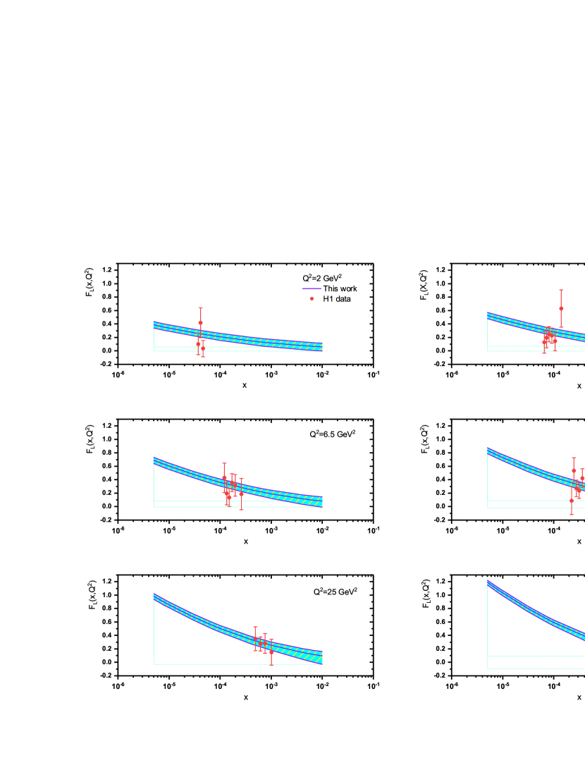
Figure 1: The longitudinal structure function extracted in comparison with the H1 data [1] as accompanied with total errors. The results are presented at fixed value of the inelasticity y ($y=0.49$). Combined H1 data for $E_{p}=460$ and $575~{}\mathrm{GeV}$ gives $\sqrt{s}=225~{}\mathrm{GeV}$. The error bands correspond to the uncertainty in the parameterization of $F_{2}(x,Q^{2})$ in [12].

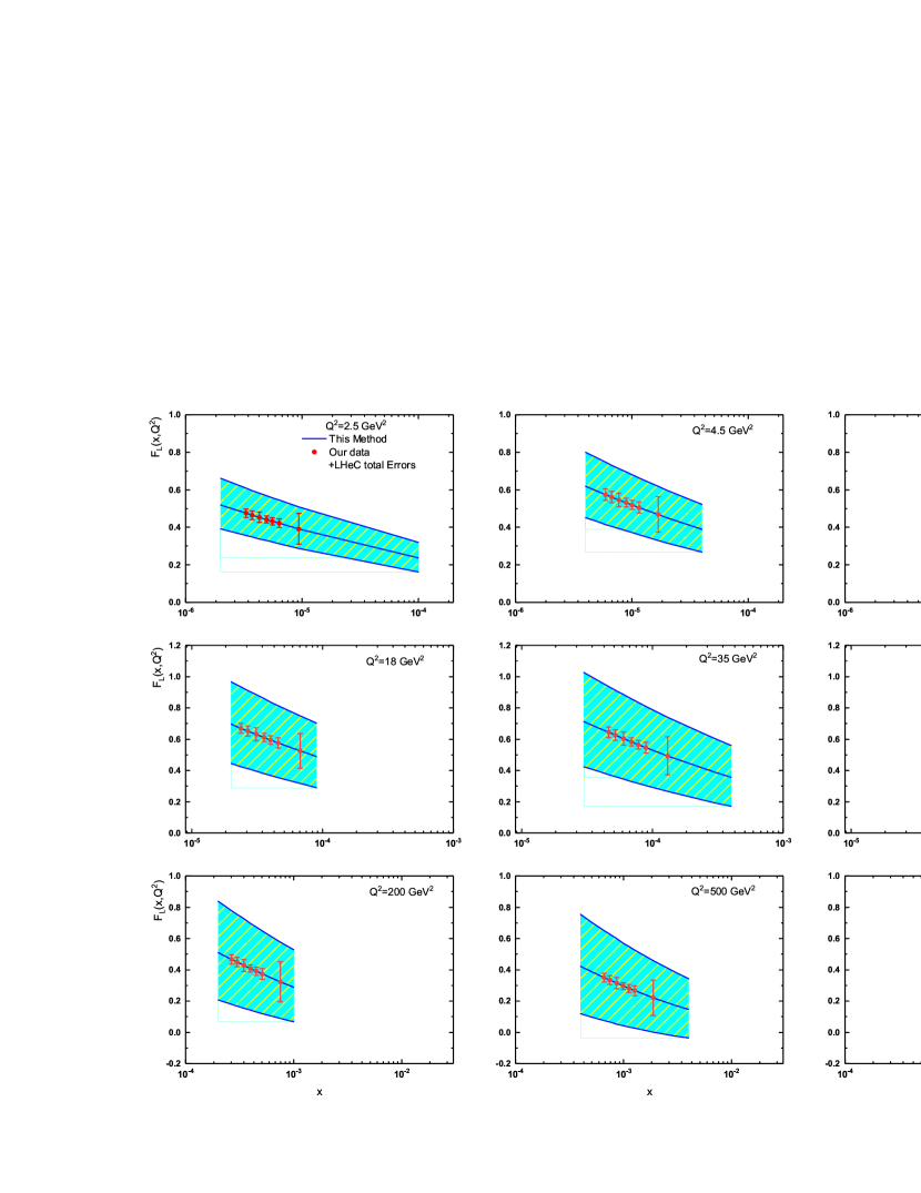
Figure 2: The longitudinal structure function extracted at low $x$ in comparison with central our data as accompanied with the LHeC total errors described in the CERN-ACC-Note-2020-0002 [3]. The results are presented in the interval values of $Q^{2}$ (i.e., $2.5~{}\mathrm{GeV}^{2}{\leq}Q^{2}{\leq}2000~{}\mathrm{GeV}^{2}$). The error bands correspond to the uncertainty in the parameterization of $F_{2}(x,Q^{2})$ in [12].

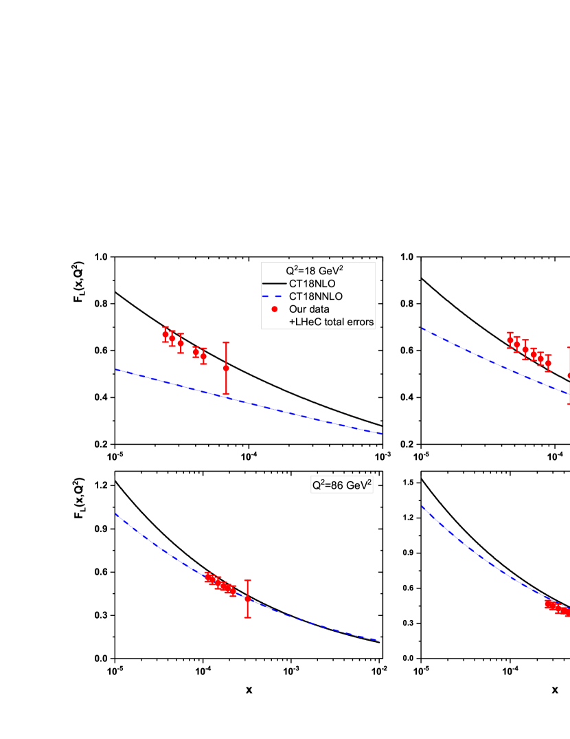
Figure 3: The longitudinal structure function $F_{L}(x,Q^{2})$ with respect to the LHeC simulated errors [3] in comparison with the results of CT18 model [44] at $Q^{2}$ values $18$, $32$, $86$ and $200~{}\mathrm{GeV}^{2}$.

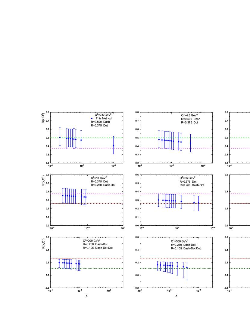
Figure 4: Predictions of the ratio $R(x,Q^{2})$ over a wide range of $Q^{2}$ values (i.e., $2.5{\leq}Q^{2}{\leq}2000~{}\mathrm{GeV}^{2}$) compared with other results. Dash, Dot, Dash-Dot and Dash-Dot Dot lines are the constant values in [45-51].

In this section, we present our results that have been obtained for the longitudinal structure function $F_{L}(x,Q^{2})$ and reduced cross section $\sigma_{r}(x,Q^{2})$ from data mediated by the parameterization of $F_{2}(x,Q^{2})$. Then we present the results obtained for $F_{L}(x,Q^{2})$ and $\sigma_{r}(x,Q^{2})$ with and without considering the HT effects. We have calculated the $Q^{2}$-dependence of the longitudinal structure function and reduced cross section with respect to the standard representations for the QCD couplings [39-41] at low values of $x$. The results for the longitudinal structure function are presented in Fig.1 and compared with the H1 data [1] as accompanied with total errors. Calculations have been performed at fixed values of the singlet and gluon exponents as they are controlled by Pomeron exchange [42,43]. In this figure (i.e., Fig.1) and the rest, the error bands represent the upper and lower limit of the uncertainty shown in Table I. As can be seen in this figure (i.e., Fig.1), the results are comparable with the H1 data in the interval $1.5~{}\mathrm{GeV^{2}}<Q^{2}<120~{}\mathrm{GeV^{2}}$. At all $Q^{2}$ values, the extracted longitudinal structure functions are in good agreement with the simulated data.
In Fig.2 our calculations for the longitudinal structure function are associated with the LHeC simulated uncertainties [3]. These simulated uncertainties for $F_{L}$ measurement recently published by the LHeC study group and reported by Ref. [3]. Indeed in Fig.2 a comparison between the statistical errors described in the parameterization method and the simulated uncertainties for the longitudinal structure function is shown along with the results of the central $F_{L}$. These comparisons are shown in the interval $2.5~{}\mathrm{GeV}^{2}{\leq}Q^{2}{\leq}2000~{}\mathrm{GeV}^{2}$ as described in [3]. In order to present more detailed discussions on our findings, we also compare the results for the longitudinal structure function with CT18 [44] in Fig.3. As can be seen from the related figures, the longitudinal structure function results are consistent with the CT18 NLO at moderate and large values of $Q^{2}$. These results are comparable to the CT18 NLO results and different from NNLO results at moderate $Q^{2}$ values. This is predictable because for CCFR and NuTeV kinematics, the difference between the NNLO results of the fixed flavor number scheme (FFNS) and each variable flavor number scheme (VFNS) is expected to be significant less than the accuracy of experimental data. Indeed at NNLO the gluon becomes more negative for very small values of $x$. The fact that the gluon is not directly physical is well-illustrated by the third-order of the longitudinal coefficient functions. At lowest and moderate $Q^{2}$ values we expect the NLO and NNLO predictions to be different in comparison with the high $Q^{2}$ in some regions.
In this figure (i.e., Fig.3) the straight lines represent the CT18 NLO and CT18 NNLO QCD analysis and the red circles represent our results as accompanied with the LHeC simulated uncertainties. Indeed the CT18 PDFs are an updated version of the CT14 [45]. Other CT18 versions, such as CT18A, Z and X, have differences in the renormalization scale and coupling constant. Corresponding to the value of $Q^{2}$, schemes such as general- mass variable flavor number scheme (GM-VFNS) and zero-mass variable flavor number scheme (ZM-VFNS) are examined by considering the production threshold of charm and bottom-quarks. The fixed flavor number scheme is valid for $Q^{2}{\lesssim}m^{2}_{H}$ and ZM-VFNS is valid for $Q^{2}{\gg}m^{2}_{H}(H=c,b)$. For realistic kinematics we used the GM-VFNS which is similarly to the ZM-VFNS in the $Q^{2}/m^{2}_{H}{\rightarrow\infty}$ limit for the CT18 results.
We found slightly disagreements between $x$-space results calculated from the parameterization method and the CT18 analysis at moderate $Q^{2}$ values for the longitudinal structure function. In fact, one of the differences is related to the shape of the introduced distribution functions. The parton distribution functions in the CT18 at the initial scale $Q_{0}^{2}$ are parametrized by Bernstein polynomials multiplied by the standard $x^{a}$ and $(1-x)^{b}$ factors that determine the small-$x$ and large-$x$ asymptotics [44]. These polynomials are very flexible across the whole interval $0<x<1$. While we have used a single power law behavior for distribution functions. Another point in the CT18 global analysis is that the starting scale $Q^{2}_{0}$ for evolution of the PDFs is around $1.69~{}\mathrm{GeV^{2}}$ in comparison with the initial scale of the parameterization method which it is almost $0.10~{}\mathrm{GeV^{2}}$. Indeed the parton distribution functions of CT18 determined using the LHC data and the combined HERA I+II data sets, along with the data sets presented in the CT14 global QCD analysis [45].
In Fig.4 the ratio of the longitudinal to transverse cross sections $R(x,Q^{2})=\sigma_{L}(x,Q^{2})/\sigma_{T}(x,Q^{2})$ is plotted in a wide range of $Q^{2}$ values. This ratio is expressed in terms of the longitudinal-to-transverse ratio of structure functions as defined by

$$R(x,Q^{2}) = \frac{F_{L}(x,Q^{2})}{F_{2}(x,Q^{2})-F_{L}(x,Q^{2})}$$ (46)

$$=\frac{\mathcal{R}(\digamma_{i,j}(x,Q^{2}))}{1-\mathcal{R}(\digamma_{i,j}(x,Q^{2}))}$$

$$=\left\{\begin{array}[]{cc}\frac{Eq.(23)}{1-Eq.(23)}&\mathrm{parameterization~{}of~{}F_{2}}\\ \\ \frac{Eq.(28)}{1-Eq.(28)}&\mathrm{effective~{}exponent}\end{array}\right\}$$

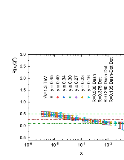
Figure 5: Ratio $R(x,Q^{2})$ plotted as a function of $x$ variable at $\sqrt{s}=1.3~{}\mathrm{TeV}$ in a wide range of $0.1{<}y{<}0.5$ compared with the dipole upper bounds [45-51].

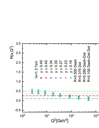
Figure 6: The same as Fig.5 for the ratio $R$ vs $Q^{2}$.

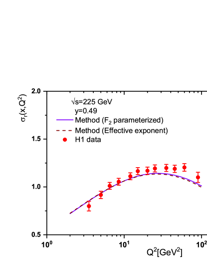
Figure 7: The reduced cross section extracted in comparison with the H1 data [1] as accompanied with total errors. The results are presented at fixed value of the inelasticity y ($y=0.49$). Combined data for $E_{p}=460$ and $575~{}\mathrm{GeV}$ give $\sqrt{s}=225~{}\mathrm{GeV}$. These results are based on two methods: the parameterization of $F_{2}$ [12] and the effective exponent [24].

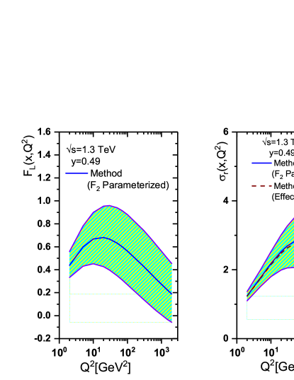
Figure 8: The longitudinal structure function (Left: $F_{L}$) and the reduced cross section (Right: $\sigma_{r}$) extracted at $\sqrt{s}=1.3~{}\mathrm{TeV}$. The averaged value of inelasticity has the value $y=0.49$.

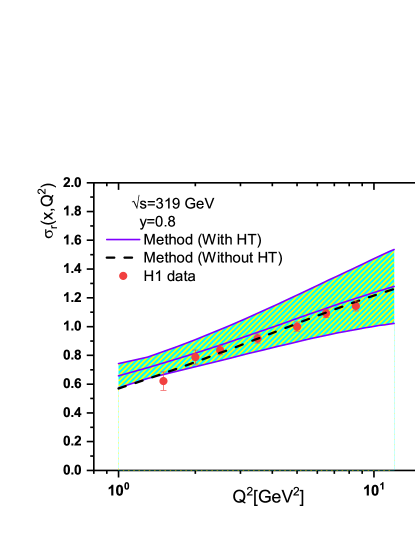
Figure 9: The reduced cross section extracted in comparison with the H1 data [1] at low $Q^{2}$ values with and without the HT corrections. The results are presented at $y=0.8$ and $\sqrt{s}=319~{}\mathrm{GeV}$. The error band corresponds to the uncertainty in the parameterization of $F_{2}$ in [12].

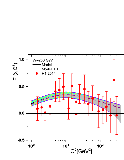
Figure 10: The longitudinal structure function extracted with and without HT corrections in comparison with the H1 data [51] as accompanied with total errors. The results are presented at fixed value of the invariant mass W ($W=230~{}\mathrm{GeV}$) at low values of $x$.

In this figure we present this ratio in comparison with the color dipole model (CDM) results [46,47,48] and experimental data [49,50]. The value of the ratio cross sections $R$ predicted to be $0.5$ or $0.375$ related to the color-dipole cross sections in Refs.[46,23,48]. H1 and ZEUS collaborations in Refs.[49,50] show that the ratio $R$ is found to be $R=0.260{\pm}0.050$ at $3.5{\leq}Q^{2}{\leq}45~{}\mathrm{GeV}^{2}$ and $0.105^{+0.055}_{-0.037}$ at $5{\leq}Q^{2}{\leq}110~{}\mathrm{GeV}^{2}$ respectively. In Fig.4, we compared our results with the other results mentioned in the literature [46-50]. We observe that the behavior of $R$ is very little dependent on $x$ and $Q^{2}$ in a wide range of $x$ and $Q^{2}$ values. This behavior is observable in comparison with the experimental data. In figures 5 and 6, the ratio of $R$ have been depicted at fixed value of the center-of-mass energy $s$ (i.e., $\sqrt{s}=1.3~{}\mathrm{TeV}$). As can be seen in these figures, the results are comparable with other constant values in the interval $0.1{<}y{<}0.5$. In Fig.6 we observe that the ratio $R$ for $\sqrt{s}=1.3~{}\mathrm{TeV}$ is consistent with a constant behavior with respect to inelasticity $y$ for fixed values of $Q^{2}$.
The determination of the structure function $F_{L}$ can be used to determine the reduced cross section $\sigma_{r}$. The $Q^{2}$-evolution results of the reduced cross section $\sigma_{r}$ are depicted in Fig.7. These results compared with the H1 data [1] correspond to the parameterization of $F_{2}$ [12] and the effective exponent [24] respectively. In both methods ($F_{2}$ parameterized and effective exponent) we find that the results are comparable with the H1 data at fixed value of the inelasticity $y=0.49$ and at a center-of-mass energy $\sqrt{s}=225~{}\mathrm{GeV}$.
This method persuades us that the obtained results can be pertinent in future analysis of the ultra-high energy neutrino data. The result of this study is shown in Fig.8. The center-of-mass energy $\sqrt{s}=1.3~{}\mathrm{TeV}$ used in accordance with the LHeC center-of-mass energy. Also the averaged parameter $y$ is constrained by the equality $<y>=0.49$. The longitudinal structure function and the reduced cross section are predicted in this energy. These results accompanied with the statistical errors of the parameterization of $F_{2}$ at $2.5{\leq}Q^{2}{\leq}2000~{}\mathrm{GeV}^{2}$ have been shown in this figure (i.e., Fig.8). Also the difference between the central values of the reduced cross sections due to the parameterization of $F_{2}$ and effective exponent methods has been shown in this figure.
In Fig.9, our reduced cross sections have been shown as a function of $Q^{2}$ values at low $x$ values with and without the HT corrections. The effect of the HT contribution to $\sigma_{r}$ can be seen from this figure. Indeed, the HT corrections lead to large corrections for low $Q^{2}$ values. We compare these results for the reduced cross section with the H1 data [1] for some selected values of low $Q^{2}$ at a center-of-mass energy $\sqrt{s}=319~{}\mathrm{GeV}$ and a fixed inelasticity value $y=0.8$. From the data versus model comparisons, the difference between our results with and without the HT corrections can be clearly be observed. In Fig.10 the results for the longitudinal structure function $F_{L}(x,Q^{2})$ have been shown with and without HT corrections at fixed value of the invariant mass W (i.e. $W=230~{}\mathrm{GeV}$) at low values of $x$. As can be seen in this figure, the results are comparable with the H1 data [51] at all $Q^{2}$ values. In comparison with the H1 data we observe that the results with the HT corrections are better than the results without the HT corrections at low values of $Q^{2}$. One can see that the differences between theory and data are decreased by including HT effects in the analysis.

.7 VII. Summary

In conclusion, we have computed the longitudinal structure function $F_{L}$ using the parameterization of $F_{2}$ to find an analytical solution for the DGLAP evolution equations. The obtained explicit expression for the longitudinal structure function is determined by parameterized the transversal proton structure function. Then we present a further development of the method of extraction of the reduced cross section from the parameterization of $F_{2}$ and $F_{L}$. The calculations are consistent with the H1 data from HERA collider.
In this work, we also calculated the longitudinal structure function and reduced cross section using the effective exponent measured by the H1 collaboration. At low $x$, the exponent $\lambda$ has been observed to increase linearly with $\ln{Q^{2}}$. In this regard, data has been collected in the kinematic range $3.10^{-5}\leq x\leq 0.2$ and $1.5\leq Q^{2}\leq 150~{}\mathrm{GeV}^{2}$. We observed that the general solutions are in satisfactory agreements with the available experimental data at a center-of-mass energy $\sqrt{s}=225~{}\mathrm{GeV}$ and a fixed value of inelasticity $y=0.49$. Our analysis is also enriched with the higher twist (HT) corrections to the reduced cross section at a center-of-mass energy $\sqrt{s}=319~{}\mathrm{GeV}$ and a fixed value of inelasticity $y=0.8$, which extend to small values of $Q^{2}$. It has been demonstrated that the HT terms are required for the low values of $Q^{2}$.
This persuades us that the obtained results can be extended to high energy regime in new colliders (like in the proposed LHeC and FCC-eh colliders). The $F_{L}$ measurements, as for LHeC, are much more precise than the initial H1 measurement and extend to lower $x$ and higher $Q^{2}$. These measurements will shed light on the parton dynamics at small $x$. When confronted with the DGLAP based predictions, one will explore the evolution dynamics deeply and more reliably than HERA measurements did allow.

.8 ACKNOWLEDGMENTS

The authors are especially grateful to Max Klein for carefully reading the manuscript and fruitful discussions. The authors are thankful to the Razi University for financial support of this project. Also G.R.Boroun thank M.Klein and N.Armesto for allowing access to data related to simulated errors of the longitudinal structure function at the Large Hadron Electron Collider (LHeC). Authors would like to thank H.Khanpour for help with preparation of the QCD parametrization models.

Table 1: The effective parameters at low $x$ for $0.15~{}\mathrm{GeV}^{2}<Q^{2}<3000~{}\mathrm{GeV}^{2}$ provided by the following values. The fixed parameters are defined by the Block-Halzen fit to the real photon-proton cross section as $M^{2}=0.753\pm 0.068~{}\mathrm{GeV}^{2}$ and $\mu^{2}=2.82\pm 0.290~{}\mathrm{GeV}^{2}$.

parameters                    value
$a_{00}$	$2.550\times 10^{-1}~{}\pm 1.60\times 10^{-2}$
$a_{01}$	$1.475\times 10^{-1}~{}\pm 3.025\times 10^{-2}$
$a_{10}$	$8.205\times 10^{-4}~{}~{}\pm 4.62\times 10^{-4}$
$a_{11}$	$-5.148\times 10^{-2}\pm 8.19\times 10^{-3}$
$a_{12}$	$-4.725\times 10^{-3}\pm 1.01\times 10^{-3}$
$a_{20}$	$2.217\times 10^{-3}\pm 1.42\times 10^{-4}$
$a_{21}$	$1.244\times 10^{-2}\pm 8.56\times 10^{-4}$
$a_{22}$	$5.958\times 10^{-4}\pm 2.32\times 10^{-4}$
$n$	$11.49\pm 0.99$
$\lambda$	$2.430~{}\pm 0.153$
$\chi^{2}(\mathrm{goodness~{}of~{}fit})$	$0.95$

I References

1. F.D. Aaron et al. [H1 Collaboration], Eur.Phys.J.C71,1579(2011); S. Chekanov et al. [ZEUS Collaboration], Phys.Lett.B682, 8(2009).
2. M.Klein, arXiv [hep-ph]:1802.04317; M.Klein, Ann.Phys.528, 138(2016); N.Armesto et al., Phys.Rev.D100, 074022(2019); F.Hautmann, LHeC 2019 workshop (https://indico-cern.ch/event/835947)(2019).
3. J.Abelleira Fernandez et al., [LHeC Collaboration], J.Phys.G39, 075001(2012); P.Agostini et al. [LHeC Collaboration and FCC-he Study Group ], CERN-ACC-Note-2020-0002, arXiv:2007.14491 [hep-ex] (2020).
4. F.Aaron et al., [H1 and ZEUS Collaborations], JHEP1001, 109(2010); J.Breitweg et al., [ZEUS Collaboration], Phys.Lett.B407, 432(1997); J.Breitweg et al., [ZEUS Collaboration], Phys.Lett.B487, 53(2000).
5. A. Abada et al., [FCC Collaboration], Eur.Phys.J.C79, 474(2019); R.A.Khalek et al., SciPost Phys.7, 051(2019).
6. A.Caldwell and M.Wing, Eur.Phys.J.C76, 463(2016); A.Caldwell et al., arXiv[hep-ph]:1812.08110(2018).
7. L.P.Kaptari et al., JETP Lett.109, 281(2019); L.P.Kaptari et al., Phys.Rev.D99, 096019(2019).
8. G.R.Boroun, Phys.Rev.C97, 015206 (2018); B.Rezaei and G.R.Boroun, Eur.Phys.J.A56, 262(2020).
9. A.V.Kotikov and G.Parente, JHEP85, 17(1997); A.V.Kotikov and G.Parente, Mod.Phys.Lett.A12, 963(1997); A.M.Cooper-Sarkar et al., Z.Phys.C39, 281(1988); A.M.Cooper-Sarkar et al., Acta Phys.Pol.B34, 2911(2003).
10. G.R.Boroun and B.Rezaei, Eur.Phys.J.C72, 2221(2012); B.Rezaei and G.R.Boroun, Nucl.Phys.A857, 42(2011); G.R.Boroun, B.Rezaei and J.K.Sarma, Int.J.Mod.Phys.A29, 1450189(2014); H.Khanpour, M.Goharipour and V.Guzey, Eur.Phys.J.C78, 1(2018).
11. N.Baruah, N.M. Nath, J.K. Sarma , Int.J.Theor.Phys.52, 2464(2013).
12. M.M.Block et al., Phys.Rev.D89, 094027 (2014).
13. E.A. Kuraev, L.N. Lipatov and V.S. Fadin, Phys. Lett. B60, 50(1975); Sov. Phys. JETP 44, 443(1976); Sov. Phys. JETP 45, 199(1977); Ya. Ya. Balitsky and L.N. Lipatov, Sov. J. Nucl. Phys.28, 822(1978).
14. B.Badelek et al., J.Phys.G22, 815(1996); S. Catani and F. Hautmann, Nucl.Phys.B427, 475(1994).
15. B.I.Ermolaev and S.I.Troyan, Eur.Phys.J.C80, 98(2020); M.Devee, R.Baishya and J.K.sarma, Eur.Phys.J.C72, 2036(2012).
16. G.R.Boroun and B.Rezaei, Eur.Phys.J.C73, 2412(2013).
17. G.Altarelli and G.Martinelli, Phys.Lett.B76, 89(1978).
18.Yu.L.Dokshitzer, Sov.Phys.JETP 46, 641(1977); G.Altarelli and G.Parisi, Nucl.Phys.B 126, 298(1977); V.N.Gribov and L.N.Lipatov, Sov.J.Nucl.Phys. 15, 438(1972).
19. S.Moch, J.A.M.Vermaseren, A.Vogt, Phys.Lett.B 606, 123(2005).
20. W.L. van Neerven, A.Vogt, Phys.Lett.B 490, 111(2000); A.Vogt, S.Moch, J.A.M.Vermaseren, Nucl.Phys.B 691, 129(2004).
21. C.Lopez and F.J.Yndurain, Nucl.Phys.B171, 231 (1980).
22. U.D^,Alesio et al., Eur.Phys.J.C9, 601 (1999); J.R.Cudell, A.Donnachie and P.V.Landshoff, Phys.Lett.B448, 281(1999); P.V.Landshoff, arXiv:hep-ph/0203084.
23. R.D.Ball et al., Eur.Phys.J.C76, 383(2016).
24. M.Praszalowicz, Phys.Rev.Lett.106, 142002(2011); M.Praszalowicz and T.Stebel, JHEP.03, 090(2013).
25. B.Rezaei and G.R.Boroun, Eur.Phys.J.A55, 66(2019).
26. A.D.Martin, W.J.Stirling and R.G.Roberts, Phys.Rev.D50, 6734(1994).
27. R.D.Ball and S.Forte, Phys.Lett.B335, 77(1994); R.D.Ball and S.Forte, Phys.Lett.B336, 77(1994).
28. D.Britzger et al., Phys. Rev. D 100, 114007 (2019).
29. C.Adloff et al. [H1 Collaboration], Phys.Lett.B520, 183(2001).
30. M. Froissart, Phys. Rev. 123, 1053 (1961).
31. M. M. Block and F. Halzen, Phys.Rev.Lett.107, 212002(2011); M. M. Block and F. Halzen, Phys. Rev. D70, 091901(2004).
32. G.R.Boroun, Lithuanian Journal of Physics 48, 121 (2008); G.R.Boroun and B.Rezaei, Phys.Atom.Nucl.71, 1077 (2008); B.Rezaei and G.R.Boroun, Eur.Phys.J. A55, 66(2019); G.R.Boroun, Eur. Phys. J. Plus 135, 68 (2020); G.R.Boroun and B.Rezaei, Acta. Phys. Slovaca 56, 463 (2006).
33. J.Blumlein and H.Bottcher, arXiv[hep-ph]:0807.0248(2008); M.R.Pelicer et al., Eur.Phys.J.C79, 9(2019).
34. A.M.Cooper-Sarkar, arXiv:1605.08577v1 [hep-ph] 27 May 2016; I.Abt et.al., arXiv:1604.02299v2 [hep-ph] 11 Oct 2016.
35. F.D. Aaron et al. [H1 Collaboration], Eur.Phys.J. C63, 625(2009).
36. H.Khanpour, A.Mirjalili and S.Atashbar Tehrani Phys.Rev.C95, 035201(2017).
37. G.R.Boroun and B.Rezaei, Nucl.Phys.A990, 244(2019); B.Rezaei and G.R.Boroun, Nucl.Phys.A1006, 122062(2021).
38. J.Lan et al., arXiv[nucl-th]:1907.01509 (2019); J.Lan et al., arXiv[nucl-th]:1911.11676 (2019).
39. B.G. Shaikhatdenov, A.V. Kotikov, V.G. Krivokhizhin, G. Parente, Phys. Rev. D 81, 034008(2010).
40. S. Chekanov et al. [ZEUS Collaboration], Eur. Phys. J. C21, 443 (2001).
41. A.D.Martin et al., Phys.Letts.B604, 61(2004).
42. A.Donnachie and P.V.Landshoff, Phys.Lett.B 437, 408(1998 ); A.Donnachie and P.V.Landshoff, Phys.Lett.B 550, 160(2002 ).
43. K Golec-Biernat and A.M.Stasto, Phys.Rev.D 80, 014006(2009).
44. Tie-Jiun Hou et al., Phys.Rev.D103, 014013(2021).
45. S.Dulat et al., Phys. Rev. D93, 033006 (2016).
46. M.Kuroda and D.Schildknecht, Phys.Lett. B618, 84(2005); M.Kuroda and D.Schildknecht, Acta Phys.Polon. B37, 835(2006); M.Kuroda and D.Schildknecht, Phys.Lett. B670, 129(2008); M.Kuroda and D.Schildknecht, Phys.Rev. D96, 094013(2017).
47. D.Schildknecht and M.Tentyukov, arXiv[hep-ph]:0203028; M.Kuroda and D.Schildknecht, Phys.Rev. D85, 094001(2012).
48. B.Rezaei and G.R.Boroun, Phys.Rev.C 101, 045202 (2020).
49. F.D. Aaron et al. [H1 Collaboration], phys.Lett.B665, 139(2008).
50. H.Abromowicz et al. [ZEUS Collaboration], Phys.Rev.D9, 072002(2014).
51. V.Andreev et al. [H1 Collaboration], Eur.Phys.J.C74, 2814 (2014).