Nonparametric estimation of copulas and copula densities by orthogonal projections

Abstract

In this paper we study nonparametric estimators of copulas and copula densities. We first focus our study on a copula density estimator based on polynomial orthogonal projections of the joint density. A new copula estimator is then deduced simply by integration. Both estimators are based on a characteristic sequence of the copulas, which we refer to as the copula coefficients. Their asymptotic properties are reviewed and a data driven selection of the number of coefficients allows these estimators to be well adapted to all types of copulas. In particular, this selection procedure perfectly detects the cases of independence. An intensive simulation study shows the very good performance of both copulas and copula densities estimators in comparison to a large panel of competitors. Applications in actuarial science illustrate this approach.

1 Introduction

Consider a $d$-random vector $\mathbf{X}=(X_{1},\cdots,X_{d})^{T}$ with joint distribution function $H$ and marginal distribution functions $F_{1},\cdots,F_{d}$, that we assumed to be continuous. According to Sklar’s Theorem (Sklar,, 1959), there exists a unique $d$-variate function $C$ such that

$$H(x_{1},\cdots,x_{d}) = C(F_{1}(x_{1}),\cdots,F_{d}(x_{d})).$$ (1)

The function $C$ is called the copula associated to $\mathbf{X}$. The copula is a joint distribution function on $I^{d}=[0,1]^{d}$, with uniform margins and satisfying $C(u_{1},\cdots,u_{d})=H(F_{1}^{-1}(u_{1}),\cdots,F_{d}^{-1}(u_{d}))$, where, for $j=1,\cdots,d$, $F^{-1}_{j}(u_{j})=\inf\{x_{j};F_{j}(x_{j})\geq u_{j}\}$, is the quantile function of $F_{j}$. Assuming that for $j=1,\cdots,d$, $F_{j}$ is differentiable, we can express the joint density $h$ of $\mathbf{X}$ (with respect to the Lebesgue measure on $I^{d}$) as

$$h(x_{1},\cdots,x_{d})=c\left(F_{1}(x_{1}),\cdots,F_{d}(x_{d})\right)\prod_{j=1}^{d}f_{j}(x_{j}),$$

where for $j=1,\cdots,d$, $f_{j}$ is the marginal density of ${X_{j}}$ and where

$$c = \frac{\partial^{d}C}{\partial x_{1}\cdots\partial x_{d}},$$

is called the copula density of $\mathbf{X}$.

Copulas and copulas density have a large spectra of applications as described for instance in Joe, (2014). They are largely used as a tool to identify a wide variety of properties such as tail-dependencies, heavy-tail, asymmetries or the heavy-tail behaviour. Copula estimation has given rise to numerous works. In parametric approaches maximum likelihood estimation is commonly used, with a general two-stage procedure as in Ko and Hjort, (2019), or penalized likelihood as in Qu and Yin, (2012), and more recently for Archimax copulas in Chatelain et al., (2020) . Such parametric methods can suffer from restrictive specification errors with few parameters. Nonparametric copula estimations generally offer a more flexible alternative and in such framework copulas density estimators have been studied with different methods: empirical processes (see Deheuvels,, 1979), kernel estimators (see for instance Geenens et al.,, 2017; Omelka et al.,, 2009) where the authors proposed a robust method, B-spline estimators (Kauermann et al.,, 2013), Bernstein polynomials (Bouezmarni et al.,, 2010, 2013), linear wavelet estimators (see Genest et al.,, 2009), nonlinear wavelet estimators (see Autin et al.,, 2010) or Legendre multiwavelet estimators (see Chatrabgoun et al.,, 2017).

In this paper we first propose to revisit the nonparametric method for estimating copula densities by considering an orthogonal shifted Legendre polynomials expansion. In this sense, our approach lies between the Legendre multiwavelet procedure and the Bernstein method. More precisely, the basic idea developed here is to consider the transformations $U_{j}=F_{j}(X_{j})$, for $j=1,\cdots,d$, which yield to a vector of uniform random variables denoted by

$$\mathbf{U}=(U_{1},\cdots,U_{d})^{T}.$$

Its joint distribution function has the form

$$H_{\mathbf{U}}(u_{1},\cdots,u_{d}) =H(F_{1}^{-1}(u_{1}),\cdots,F_{d}^{-1}(u_{d})),$$

and clearly, $\mathbf{U}$ and $\mathbf{X}$ have the same structure of dependence with the same copula. We deduce that

$$h_{\mathbf{U}}(u_{1},\cdots,u_{d}) =c(u_{1},\cdots,u_{d}),$$ (2)

where $h_{\mathbf{U}}$ denotes the joint density of $\mathbf{U}$ with respect to the Lebesgue measure on $[0,1]^{d}$. This basic equality is the start of the construction of the copula density estimator, expressing $c$ in a basis of orthogonal polynomials. In addition, a new copula estimator is derived by simply integrating the polynomial expansion. Both estimators are based on a characteristic sequence of the copulas, which we refer to as the copula coefficients. The properties of these estimators are studied: the copula density estimator satisfies the uniform margins property (see Proposition 3) that almost all nonparametric estimators in the literature suffer. Various asymptotic properties are reviewed for both estimators. We also provide a functional class for which the construction of the copula estimator is optimal in the minimax sense. We propose a data driven method of selection for the number of projections. In the case of independence this criteria can find the exact form of the copula and our estimator then seems to greatly surpass all the other competitors. Moreover, a relation between the Spearman’s rho $\rho_{C}$ and the copula coefficients is highlighted, yielding to a new estimator of $\rho_{C}$. Finally, both estimators seem to outperform all others known in the statistical literature for a wide spectrum of scenarios. Moreover, these estimators are very simple and easy to implement and their execution time is very fast. Their interest is also demonstrated on a real dataset.

The paper is organised as follows. In section 2 we develop the methodology of the estimation procedure. Section 3 is devoted to the elementary and asymptotic properties with minimax results. A selection method of the number of expansion components and a numerical comparison with other nonparametric estimators are proposed in Section 4. Section 5 is devoted to two applications on real actuarial dataset. Finally in Section 6 we discuss further leads of research connected with copula estimation and we explain why our approach is efficient even without square integrability assumption. All proofs are relegated to the Appendix.

2 Construction of the estimators

Let us denote by $\mu$ the uniform measure on $\displaystyle I=[0,1]$ and by $\{Q_{m};m\in\mathbb{N}\}$ an orthonormal basis of shifted Legendre polynomials satisfying

$$\displaystyle\int_{I}Q_{m}(x)Q_{k}(x)\mu(dx) = \delta_{mk},$$

with $\delta_{mk}=1$ if $m=k$ and $0$ otherwise. The orthonormal shifted Legendre polynomials $\displaystyle Q_{m}$ are defined on $\displaystyle I$ by

$$\displaystyle Q_{m}(x)=\sqrt{2m+1}L_{m}(2x-1),$$

where $L_{m}$ are the well known classical Legendre polynomials defined by

$$L_{0}=1;L_{1}(x)=x; {\rm and} (m+1)L_{m+1}(x)=(2m+1)xL_{m}(x)-mL_{m-1}(x).$$

Characterizations and properties of Legendre polynomials can be found in Abramowitz and Stegun, (1970). For all $\mathbf{x}=(x_{1},\cdots,x_{d})^{T}\in I^{d}$ and for all $\mathbf{m}=(m_{1},\cdots,m_{d})^{T}\in\mathbb{N}^{d}$, we define

$$\mathbf{Q}_{\mathbf{m}}(\mathbf{x}) = \prod_{j=1}^{d}Q_{m_{j}}(x_{j}),$$

and we write

$$\rho_{\mathbf{m}} = \mathbb{E}\left(\prod_{j=1}^{d}Q_{m_{j}}(F_{j}(X_{j}))\right).$$ (3)

The following assumption will be used throughout the paper and says that the copula density $c$ belongs to $\mathbb{L}^{2}([0,1]^{d})$

$$\displaystyle\lVert c\rVert_{2}^{2}=\sum_{{\mathbf{m}}\in\mathbb{N}^{d}}\rho_{\mathbf{m}}^{2}<\infty,$$ (4)

where $\lVert.\rVert_{2}$ denotes the norm with respect to the Lebesgue measure on $[0,1]^{d}$.

Assumption (4) is obviously satisfied for any bounded copula density, for instance the Farlie-Gumbel-Morgenstern and Frank copula densities (see Nelsen, (2007) for definitions). Beare, (2010) showed that $\displaystyle\lVert c_{\rho}\rVert_{2}^{2}=(1-\rho^{2})^{-1/2}$ for the standard bivariate Gaussian copula density with correlation coefficient $\rho\in(0;1)$. Moreover, Beare, (2010) noted that in the bivariate case, copulas associated to Lancaster type distributions (Lancaster,, 1958) satisfied (4). This is the case for bivariate gamma, Poisson, binomial and hypergeometric distributions, and for the compound correlated bivariate Poisson distribution (see for instance Hamdan and Al-Bayyati, (1971)). However, copulas exhibiting lower or upper tail dependence (in the sense of McNeil et al., (2015)) do not have square integrable density. In particular, the Gumbel, Clayton, and t-copulas all have upper or lower tail dependence and then do not satisfy condition (4). In Appendix 7 we discuss the possibility to modify such copulas with a shrinkage factor to be square integrable and we illustrate such a procedure. This explains why our method can work so well even if (4) is not satisfied. But it is important to note that our framework is nonparametric and that the possible family of the copula is unknown.

Proposition 1

Assume that (4) holds. Then we have

$$c(u_{1},\cdots,u_{d}) = \displaystyle\sum_{\mathbf{m}\in\mathbb{N}^{d}}\rho_{\mathbf{m}}\mathbf{Q}_{\mathbf{m}}({\mathbf{u}})$$ (5)

$$C(u_{1},\cdots,u_{d}) = \displaystyle\sum_{{\mathbf{m}}\in\mathbb{N}^{d}}\rho_{{\mathbf{m}}}\prod_{j=1}^{d}\displaystyle\int_{0}^{u_{j}}Q_{m_{j}}(x_{j})\mu(dx_{j}).$$ (6)

It is important to note that the sequence $(\rho_{{\mathbf{m}}})_{{\mathbf{m}}\in\mathbb{N}^{d}}$ characterizes the copula. In this way it will be referred to as the copula coefficients. Since $Q_{0}=1$ we have $\rho_{\mathbf{0}}=1$. The particular case $\rho_{\mathbf{m}}=0$ for all $\mathbf{m}\neq 0$ coincides with the independent case. As seen in (3), the sequence $(\rho_{{\mathbf{m}}})_{{\mathbf{m}}\in\mathbb{N}^{d}}$ contains all the polynomial correlations between the marginal uniform random variables. In the bivariate case, that is when $d=2$, the element $\rho_{\mathbf{m}}$ simply expresses the correlation between $Q_{m_{1}}(F_{1}(X_{1}))$ and $Q_{m_{2}}(F_{2}(X_{2}))$. In the general case, by orthogonality, we have $\mathbb{E}\left(Q_{m_{j}}(F_{j}(X_{j}))\right)=0$ for all $m_{j}>0$ and then $\rho_{\mathbf{m}}=0$ as soon as only one component of $\mathbf{m}$ is zero. Moreover, if for some integer $j\in\{1,\cdots,d\}$, $X_{j}$ is independent to all over variables $X_{i}$, $i\neq j$, then $\rho_{\mathbf{m}}=0$ as soon as $m_{j}>0$. Then the copula coefficients can be used as an indicator of independence between the components of $\mathbf{X}$. In this sense, we also exhibit a link with the Spearman’s rho in Section 3.

For any positive integer vector ${\mathbf{N}}=(N_{1},\cdots,N_{d})^{T}$ we define the following ${\mathbf{N}}$-th order approximations:

$$c^{[\mathbf{N}]}(\mathbf{u}) = \sum_{{\mathbf{m}}\leq\mathbf{N}}\rho_{{\mathbf{m}}}\prod_{j=1}^{d}Q_{m_{j}}(u_{j})$$

$$C^{[\mathbf{N}]}(\mathbf{u}) = \displaystyle\sum_{{\mathbf{m}}\leq\mathbf{N}}\rho_{{\mathbf{m}}}\prod_{j=1}^{d}\displaystyle\int_{0}^{u_{j}}Q_{m_{j}}(x_{j})\mu(dx_{j}),$$

where the inequality ${\mathbf{m}}\leq{\mathbf{N}}$ means that $m_{j}\leq N_{j}$ for all $j=1,\cdots,d$. We write $\mathbf{m}\not\leq\mathbf{N}$ when $\mathbf{m}$ does not satisfy this inequality. If we observe a $n$-sample $\mathbf{X}_{1},\cdots,\mathbf{X}_{n}$, of iid random data, with $\mathbf{X}_{i}=(X_{i1},\cdots,X_{id})^{T}$ having joint distribution function $H$, then we can estimate the quantity $\rho_{\mathbf{m}}$ by

$$\widehat{\rho}_{{\mathbf{m}}} = \left\{\begin{array}[]{cc}\displaystyle 1&{\rm if\ }\mathbf{m}=\mathbf{0},\\ \displaystyle 0&{\rm if\ exactly\ }d-1{\rm\ components\ of\ }\mathbf{m}{\rm\ are\ zero},\\ \displaystyle\frac{1}{n}\displaystyle\sum_{i=1}^{n}\prod_{j=1}^{d}Q_{m_{j}}(\widehat{F}_{j}(X_{ij})),&{\rm else},\end{array}\right.$$

where $\displaystyle\widehat{{F}}_{j}({x})=\frac{1}{n}\sum_{i=1}^{n}\mathds{1}(X_{ij}\leq x)$.

Remark 1

Since the marginal distributions are continuous, the ties occur with probability zero. So we can also simply write

$$\widehat{\rho}_{{\mathbf{m}}} = \frac{1}{n}\displaystyle\sum_{i=1}^{n}\prod_{j=1}^{d}Q_{m_{j}}\Big{(}\frac{R_{ij}}{n}\Big{)},$$

where $R_{ij}$ denotes the rank of $X_{ij}$.

A $\mathbf{N}$-th order nonparametric estimator of the copula density $c$ is given by

$$\displaystyle\widehat{c}^{[{\mathbf{N}}]}(u_{1},\cdots,u_{d}) = \sum_{{\mathbf{m}}\leq{\mathbf{N}}}\widehat{\rho}_{{\mathbf{m}}}\prod_{j=1}^{d}Q_{m_{j}}(u_{j}).$$ (8)

By integration, we get a very simple $\mathbf{N}$-th order nonparametric estimator of the copula function as follows

$$\displaystyle\widehat{C}^{[{\mathbf{N}}]}(u_{1},\cdots,u_{d})=\sum_{{\mathbf{m}}\leq{\mathbf{N}}}\widehat{\rho}_{{\mathbf{m}}}\prod_{j=1}^{d}\displaystyle{\int_{0}^{u_{j}}Q_{m_{j}}(x_{j})\mu(dx_{j})}.$$ (9)

Remark 2

In the particular case where the margins $F_{1},\cdots,F_{d}$ are known, the pseudo-estimator of the copula coefficients is given by

$$\tilde{\rho}_{{\mathbf{m}}} = \frac{1}{n}\displaystyle\sum_{i=1}^{n}\prod_{j=1}^{d}Q_{m_{j}}(F_{j}(X_{ij})),$$

and the associated copula and copula density pseudo-estimators are

$$\displaystyle\tilde{c}^{[{\mathbf{N}}]}(u_{1},\cdots,u_{d}) = \sum_{{\mathbf{m}}\leq{\mathbf{N}}}\tilde{\rho}_{{\mathbf{m}}}\prod_{j=1}^{d}Q_{m_{j}}(u_{j}),$$

$$\displaystyle\tilde{C}^{[{\mathbf{N}}]}(u_{1},\cdots,u_{d})=\sum_{{\mathbf{m}}\leq{\mathbf{N}}}\tilde{\rho}_{{\mathbf{m}}}\prod_{j=1}^{d}\displaystyle{\int_{0}^{u_{j}}Q_{m_{j}}(x_{j})\mu(dx_{j})}.$$ (10)

Remark 3

We can see that $\widehat{c}^{[\mathbf{0}]}=1$ which coincides exactly with the copula density in the independent case. In such case, we will observe this phenomenon in our simulation study where the copula and its estimator are very often exactly the same.

3 Some properties of the estimators

Write $\bm{\mu}^{d}=\mu\times\cdots\times\mu$ the product of the uniforme measure $d$ times.

3.1 Elementary properties

Proposition 2

Let $\mathbf{u}\in I^{d}$ and fix $\mathbf{N}\in\mathbb{N}^{d}$. The copula estimator $\displaystyle\widehat{C}^{[{\mathbf{N}}]}$ given by (9) satisfies the following properties

• If at least one coordinate of $\mathbf{u}$ is zero then $\displaystyle\widehat{C}^{[{\mathbf{N}}]}({\mathbf{u}})=0$.

• If $\displaystyle\mathbf{u}=(1,\cdots,1,u_{i},1,\cdots,1)$, then $\widehat{C}^{[{\mathbf{N}}]}({\mathbf{u}})=u_{i}$.

• $\displaystyle\widehat{C}^{[{\mathbf{0}}]}({\mathbf{u}})=\prod_{j=1}^{d}u_{j}$.

Proposition 3

The copula density estimator $\displaystyle\widehat{c}^{[{\mathbf{N}}]}$ given by (8) satisfies the following properties

• $\displaystyle\int_{I^{d}}\widehat{c}^{[{\mathbf{N}}]}({\mathbf{u}})\bm{\mu}^{d}(d{\mathbf{u}})=1$.

• For all $u_{j}\in I$, $j=1,\cdots,d$, writing  $\displaystyle{\mathbf{x}_{-j}}=(x_{1},\cdots,x_{j-1},u_{j},x_{j+1},\cdots,x_{d})$, we have

  $$\displaystyle\int_{I^{d-1}}\widehat{c}^{[{\mathbf{N}}]}({\mathbf{x}_{-j}})\bm{\mu}^{d-1}(\mathrm{d}{x_{1}\cdots\mathrm{d}x_{j-1}\mathrm{d}x_{j+1}\cdots\mathrm{d}x_{d}})=1.$$

• $\displaystyle\widehat{c}^{[{\mathbf{0}}]}({\mathbf{u}})=1$, for all ${\mathbf{u}}\in I^{d}$.

Let us recall that for any continuous bivariate random variable $(X_{1},X_{2})$ with copula $C$, the Spearman’s rho can be express as (see Nelsen, (2007)):

$$\displaystyle\rho_{C}=12\int_{0}^{1}\int_{0}^{1}C(u,v)dudv-3.$$

The result below gives a simplified new expression of $\displaystyle\rho_{C}$ in terms of copula coefficients.

Proposition 4

Let $(X_{1},X_{2})$ be a continuous bivariate random variable with copula $C$. Then the Spearman’s rho coincides with the first copula coefficient defined by (3), that is:

$$\displaystyle\rho_{C}=\rho_{11}.$$

We can immediately deduce an estimator of the Spearman’s rho as follows:

$$\displaystyle\hat{\rho}_{C}=\displaystyle\hat{\rho}_{11}=\frac{3}{n}\sum_{i=1}^{n}\left(2\widehat{U}_{i1}-1\right)\left(2\widehat{U}_{i2}-1\right).$$

This estimator is new and could be compared to the ones given in Pérez and Prieto-Alaiz, (2016) but such a study exceeds the scope of this paper.

3.2 Asymptotic properties

Proposition 5

Fix $\mathbf{N}\in\mathbb{N}^{d}$, independent of $n$. For all $\mathbf{u}\in I^{d}$, we have

• $$\widehat{c}^{[{\mathbf{N}}]}({\mathbf{u}}) = \tilde{c}^{[{\mathbf{N}}]}({\mathbf{u}})+\mathcal{O}_{\mathbb{P}}\big{(}\sqrt{n^{-1}}\big{)}.$$

• $$\widehat{C}^{[{\mathbf{N}}]}({\mathbf{u}}) = \tilde{C}^{[{\mathbf{N}}]}({\mathbf{u}})+\mathcal{O}_{\mathbb{P}}\big{(}\sqrt{n^{-1}}\big{)}$$

For any integer $\mathbf{N}\in\mathbb{N}^{d}$, the notation $\mathbf{N}\to\infty$ means $N_{j}\to\infty$ for all $j=1,\cdots,d$ and the $\displaystyle\max_{j=1,\cdots,d}(N_{j})$ will be denoted by $\displaystyle N_{max}$.

We now consider the Mean Integrated Squared Error (MISE) as a rule criteria to decide which degree of approximation we use. We write

$$MISE(\widehat{c}^{[\mathbf{N}]}) = \displaystyle\mathbb{E}\|\widehat{c}^{[\mathbf{N}]}-c\|_{2}^{2}=\mathbb{E}\int_{I^{d}}\left(\widehat{c}^{[{\mathbf{N}}]}(\mathbf{u})-c(\mathbf{u})\right)^{2}\bm{\mu}^{d}(d\mathbf{u}).$$

Proposition 6

Assume that (4) holds. For all ${\mathbf{N}}\in\mathbb{N}^{d}$ we have

$$MISE(\widehat{c}^{[\mathbf{N}]}) = \mathbb{E}\left(\sum_{\mathbf{m}\leq\mathbf{N}}(\widehat{\rho}_{\mathbf{m}}-\rho_{\mathbf{m}})^{2}\right)+\displaystyle\sum_{\mathbf{m}\not\leq\mathbf{N}}\rho_{\mathbf{m}}^{2}.$$

Thus $\mathbf{N}$ represents a smoothing parameter which controls the trade-off between the bias-squared and the variance.

Corollary 1

Fix $N\in\mathbb{N}^{d}$, independent of $n$. Then we have

$$\displaystyle MISE(\widehat{c}^{[\mathbf{N}]})=MISE(\widetilde{c}^{[{\mathbf{N}}]})+\mathcal{O}(n^{-1})$$

From now on, assume that $\displaystyle{\mathbf{N}}={\mathbf{N}}(n)$ and consider the assumption

$${(\mathbf{H})} \hskip 85.35826ptN_{max}^{2d+4}=o\left(n\right).\hskip 142.26378pt$$

Corollary 2

Assume that (4) and (H) hold. The copula density estimator $\widehat{c}^{[{\mathbf{N}}]}$ is asymptotically consistent in the integrated mean squared sense, that is:

$$MISE(\widehat{c}^{[\mathbf{N}]})\xrightarrow[\enskip n\longrightarrow\infty\enskip]{}0.$$

Proposition 7

Assume that (4) and (H) hold. For any $\mathbf{u}\in I^{d}$, we have as $n\to\infty$

$$\displaystyle\mathbb{E}\left(\widehat{c}^{[{\mathbf{N}}]}(\mathbf{u})\right)\longrightarrow c(\mathbf{u}){\rm\ and\ }\mathbb{E}\left(\widehat{C}^{[{\mathbf{N}}]}(\mathbf{u})\right)\longrightarrow C(\mathbf{u})$$

3.3 Minimax results

We recall here the minimax procedure in the spirit of Goldenshluger and Lepski, (2014) or Cohen et al., (2001). of a given estimator $\widehat{c}$ over this set by its maximum risks (or worst case risk) defined as follows

$$\displaystyle\mathcal{R}(\mathcal{F})=\sup_{c\in\mathcal{F}}\mathbb{E}\|\widehat{c}-c\|^{2}_{2},$$

that we compare to a benchmark which is the following minimax risk

$$\displaystyle\mathcal{R}^{\star}(\mathcal{F},{\cal C})=\inf_{\widehat{c}\in{\cal C}}\sup_{c\in\mathcal{F}}\mathbb{E}\|\widehat{c}-c\|^{2}_{2},$$

where $\cal C$ denotes the class of the estimators $\widehat{c}$. In our case we consider the class of estimators satysfying (8) which depends of the approximation degree $\mathbf{N}$. Then we simply write

$$\displaystyle\mathcal{R}^{\star}(\mathcal{F})=\inf_{{\mathbf{N}}}\sup_{c\in\mathcal{F}}\mathbb{E}\|\widehat{c}^{[\mathbf{N}]}-c\|^{2}_{2}.$$

Denoting by $n$ the sample size, a sequence $(v_{n})$ is said to be an optimal rate convergence in the minimax sense for $\mathcal{F}$ if there exits two constants $M_{1}$ and $M_{2}$ such that

$$\displaystyle M_{1}v_{n}\leq\mathcal{R}^{\star}(\mathcal{F})\leq M_{2}v_{n},$$

and the estimator $\widehat{c}$ is said minimax optimal if there exists a constant $\Upsilon$ such that

$$\mathcal{R}(\mathcal{F})\leq\Upsilon v_{n}.$$

For more details about minimax theory we alos refer to Tsybakov, (2003) and Efromovich, (2008).

Under (4) the copula density $c$ is characterized by its sequence of copula coefficients $(\rho_{{\mathbf{m}}})_{{\mathbf{m}}\in\mathbb{N}^{d}}$, and for $\bm{\beta}=(\beta_{1},\cdots,\beta_{d})\in(\mathbb{R}_{+}^{*})^{d}$, and $0<L<\infty$, we denote by ${\mathcal{F}}_{\bm{\beta}}(L)$ the ellipsoid space defined by:

$${\mathcal{F}}_{\bm{\beta}}(L)=\left\{c\in\mathbb{L}^{2}([0,1]^{d})~{}/\displaystyle\sum_{\mathbf{m}\in\mathbb{N}^{d}}{\rho}_{\mathbf{m}}^{2}\left(1+\sum_{i=1}^{d}m_{i}^{\beta_{i}}\right)<L\right\}.$$

As discussed in Appendix 7 there are some copulas families which do not satisfy assumption (4) and then do not belong to ${\mathcal{F}}_{\bm{\beta}}(L)$. This is the case for Clayton, Gumbel or Student copulas. However, such copulas can be approximated as closely as we want by a function of this space as illustrated in Appendix 7.

The fonctionnal space ${\mathcal{F}}_{\bm{\beta}}(L)$ with assumption $c\in{\mathcal{F}}_{\bm{\beta}}(L)$ allows to control the bias term of the risk. We observe that, on the balls ${\mathcal{F}}_{\bm{\beta}}(L)$, we have

$$\|c^{[\mathbf{N}]}-c\|^{2}_{2}\leq L\sum_{j=1}^{d}N_{j}^{-\beta_{j}}.$$ (11)

Remark 4

Usually multivariate regularity spaces are defined by

$${\mathcal{\tilde{F}}}_{\bm{\beta}}=\left\{c\in\mathbb{L}^{2}(I^{d})~{}/\displaystyle\sum_{\mathbf{m}\in\mathbb{N}^{d}}{\rho}_{\mathbf{m}}^{2}\prod_{i=1}^{d}m_{i}^{\beta_{i}}<\infty\right\},$$

and equation (11) is also satisfied on the balls

$${\mathcal{\tilde{F}}}_{\bm{\beta}}(L)=\left\{c\in\mathbb{L}^{2}(I^{d})~{}/\displaystyle\sum_{\mathbf{m}\in\mathbb{N}^{d}}{\rho}_{\mathbf{m}}^{2}\prod_{i=1}^{d}m_{i}^{\beta_{i}}<L\right\}.$$

Note that all results below can also established on such spaces ${\mathcal{\tilde{F}}}_{\bm{\beta}}(L)$.

Proposition 8

Assume that (4) holds. Let $\displaystyle b^{-1}=\sum_{i=1}^{d}\frac{1}{\beta_{i}}$ and assume that the integer vector $\mathbf{N}$ satisfies

$${(\mathbf{H}^{\prime})} \hskip 85.35826ptN_{max}=\lfloor n^{\frac{1}{2d+b+4}}\rfloor,\hskip 142.26378pt$$

where $\lfloor.\rfloor$ denotes the integer part. Then for all sample size $n$ we have

$$\sup_{\displaystyle c\in{\mathcal{F}}_{\bm{\beta}}(L)}\mathbb{E}\|\widehat{c}^{[{\mathbf{N}}]}-c\|^{2}_{2} < \alpha n^{-\frac{b}{b+2d+4}},$$

where $\alpha=8(d)^{2}({3})^{d}+{2({3})^{d}}+Ld$.

Clearly, the previous condition (H’) is stronger than (H). We known that in the independent case (see Remark 4), if $\mathbf{N}=\mathbf{0}$ we have $\widehat{c}^{[\mathbf{0}]}=c$. We now exclude the case $\mathbf{N}=\mathbf{0}$ and we propose an upper bound of the minimax risk when $\displaystyle\mathcal{R}^{\star}(\mathcal{F})=\inf_{\mathbf{N}\neq\mathbf{0}}\sup_{c\in\mathcal{F}}\mathbb{E}\|\widehat{c}-c\|^{2}_{2}$.

Proposition 9

Assume that (4) holds and $\mathbf{N}\neq\mathbf{0}$. Let $v_{n}=n^{-\frac{1}{2d+b+4}}$. Then

$$\displaystyle\mathcal{R}^{\star}\left(\mathcal{F}_{\bm{\beta}}(L)\right)\leq Kv_{n},$$

where $K=\frac{Ld(2d+b+4)}{2d+4}\left(\frac{Lbd}{\eta(2d+4)}\right)^{\frac{-b}{2d+b+4}}$, with $\eta=8(d)^{2}({3})^{d}+{2({3})^{d}}.$

4 Numerical analyses and comparisons

In this section, we present simulation results which demonstrate the performance of our approach compared with a number of recent alternative estimators. All computations were performed using the R software.

Since the results depend of the degree of the approximations we first present a data driven method to select $\mathbf{N}$.

4.1 Data driven degree selection

We propose to use a data-driven procedure based on the Least-Squares Cross-Validation (LSCV) to select the optimal parameter $\displaystyle\widehat{\mathbf{N}}_{opt}$. The LSCV procedure has been introduced by Rudemo, (1982) and Bowman, (1984) to select the smoothing bandwidth for Kernel density estimation and it has been adapted to orthogonal series estimators by Taylor, (1990). In the general case, the smoothing parameter is the minimizer of the following function

$$\displaystyle LSCV({\mathbf{N}})=\int_{I^{d}}\left(\widehat{c}^{[{\mathbf{N}}]}({\mathbf{u}})\right)^{2}d{\mathbf{u}}-\displaystyle\frac{2}{m}\displaystyle\sum_{i=1}^{m}\widehat{c}^{[{\mathbf{N}}]}_{-i}\left(F_{1}(X_{i1}),\cdots,F_{d}(X_{id})\right),$$

which can be estimated by

$$\displaystyle\widehat{LSCV}({\mathbf{N}})=\int_{I^{d}}\left(\widehat{c}^{[{\mathbf{N}}]}({\mathbf{u}})\right)^{2}d{\mathbf{u}}-\displaystyle\frac{2}{m}\displaystyle\sum_{i=1}^{m}\widehat{c}^{[{\mathbf{N}}]}_{-i}\left(\widehat{F}_{1}(X_{i1}),\cdots,\widehat{F}_{d}(X_{id})\right),$$ (12)

yielding to the following estimator of $\mathbf{N}$:

$$\displaystyle\widehat{\mathbf{N}}_{opt}=\operatorname*{argmin}_{{\mathbf{N}}\in\mathbb{N}^{d}}\widehat{LSCV}({\mathbf{N}}),$$

where $\displaystyle\widehat{c}^{[{\mathbf{N}}]}_{-i}$ is the leave-one-out copula density estimator without the data point $\mathbf{X}_{i}=(X_{i1},\cdots,X_{id})$. Note that the expression (12) has a similar form as the LSCV criterion used by Bouezmarni et al., (2013).

The proposition below gives an abridged form of $\widehat{LSCV}(\mathbf{N})$ which is very useful to decrease its computation time in the numerical study.

Proposition 10

Fix $\mathbf{N}\in\mathbb{N}^{d}$. We have

$$\displaystyle\widehat{LSCV}(\mathbf{N})=\frac{1}{n^{2}}\displaystyle\sum_{\mathbf{m}\leq\mathbf{N}}\left(\sum_{i=1}^{n}\prod_{j=1}^{d}Q_{m_{j}}^{2}\Big{(}\widehat{F}_{j}(X_{ij})\Big{)}-\displaystyle\frac{n+1}{n-1}\sum_{k\neq i}\prod_{j=1}^{d}Q_{m_{j}}\Big{(}\widehat{F}_{j}(X_{ij})\Big{)}Q_{m_{j}}\Big{(}\widehat{F}_{j}(X_{kj})\Big{)}\right).$$

The form of the $\widehat{LSCV}$ given in Proposition 10 has the advantage to be easily evaluated numerically and it will be used in our simulation to select the value of $\mathbf{N}$ by minimising this expression.

Proposition 11

Fix $\mathbf{N}\in\mathbb{N}^{d}$, independent of $n$. We have

$$\displaystyle\mathbb{E}\left(\widehat{LSCV}(N)\right) = MISE(\widehat{c}^{[\mathbf{N}]})-\|c\|_{2}^{2}+\mathcal{O}(n^{-1}).$$

Remark 5

In the case where the margins are known we have

$$\displaystyle\mathbb{E}\left(\widehat{LSCV}(N)\right) = MISE(\widetilde{c}^{[{\mathbf{N}}]})-\|c\|_{2}^{2}.$$

4.2 Finite-sample performance of copula estimators

To simplify our numerical study we fix $N_{1}=\cdots=N_{d}:=N$. It is therefore still possible to gain in precision by taking the time to choose a best combination of the components of the degree approximation $\mathbf{N}$.

We use Monte Carlo simulations to demonstrate the potential of the copula estimator $\displaystyle\widehat{C}^{[{\mathbf{N}}]}$ given in (9) where the optimal parameter $\mathbf{N}$ is selected as described in Section 4.1. This estimator will be denoted by CN. We compare the performance with four competitors, namely:

• The empirical copula (Deheuvels,, 1979), denoted Emp;

• The empirical checkerboard copula (Carley and Taylor,, 2002), denoted Check;

• The empirical Bernstein copula (Sancetta and Satchell,, 2004), denoted Berns10 and Berns25 with smoothing parameter $k=10$ and $k=25$ respectively;

• The empirical beta copula (Segers et al.,, 2017), denoted Beta.

We consider the classic copulas below in bivariate and trivariate dimension in the simulation series:

• Clayton copula;

• Frank copula;

• Gaussian copula;

• Gumbel copula;

• Independence copula;

• Joe copula;

• Student t-copula with degrees of freedom $\nu=17$.

The readers may refer to Nelsen, (2007) for the explicit functional forms and properties of these copulas. We consider three levels of dependence with kendall’s $\displaystyle\tau$’s equal to $\displaystyle\tau=0.3$ (low dependence), $\displaystyle\tau=0.55$ (middle dependence) and $\displaystyle\tau=0.8$ (high dependence) for each copula model. We generate in both case iid data using each copula model of sizes $\displaystyle n=500$ and $\displaystyle n=1000$. In order to evaluate the quality of an estimator $\displaystyle\widehat{C}$ for a given copula $\displaystyle C$, we consider three performances measures: the first one is the mean integrated absolute error (MIAE), defined by

$$\text{MIAE}(\widehat{C})=\mathbb{E}\left(\int_{I^{d}}\left|\widehat{C}^{[{\mathbf{N}}]}(\mathbf{u})-C(\mathbf{u})\right|d\mathbf{u}\right),$$

the second one is the mean integrated squared error (MISE), defined by

$$\text{MISE}(\widehat{C})=\mathbb{E}\left(\int_{I^{d}}\left|\widehat{C}^{[{\mathbf{N}}]}(\mathbf{u})-C(\mathbf{u})\right|^{2}d\mathbf{u}\right),$$

and the last one is the mean Kolmogorov-Smirnov error (MK-SE) defined by

$$\text{MK-SE}(\widehat{C})=\mathbb{E}\left(\sup_{\mathbf{u}\in I^{d}}\left|\widehat{C}^{[{\mathbf{N}}]}(\mathbf{u})-C(\mathbf{u})\right|\right),$$

estimated by the average over $M=1,000$ Monte Carlo replications of the approximate integration and Kolmogorov-Smirnov distance as follows

$$\displaystyle\|\widehat{C}^{[{\mathbf{N}}]}-C\|_{p}^{2} \approx \frac{1}{T^{d}}\sum_{j_{1},\cdots,j_{d}=1}^{T-1}\left|\widehat{C}^{[{\mathbf{N}}]}({\mathbf{j}}/T)-C({\mathbf{j}}/T)\right|^{p},\,p=1,2,$$

$$\sup_{\mathbf{u}\in I^{d}}\left|\widehat{C}^{[{\mathbf{N}}]}(\mathbf{u})-C(\mathbf{u})\right| \approx \sup_{j_{1},\cdots,j_{d}=1,\cdots,T-1}\left|\widehat{C}^{[{\mathbf{N}}]}({\mathbf{j}}/T)-C({\mathbf{j}}/T)\right|,$$

where ${\mathbf{j}}/T=(j_{1}/T,\cdots,j_{d}/T)$.

Two-dimensional case.

In the case where $d=2$, Tables 1-3 display the relatives MIAE, MISE and MK-SE for the considered two sample sizes and three levels of dependence. It can be observed that the copula estimator $\widehat{C}^{[\mathbf{N}]}$ performs highly than the rest of the estimators overall on these error criteria and for different sample sizes and levels of dependence. It is important to precise some comments on the individual comparisons:

• For copulas with high dependence (Kendall’s $\tau=0.8$), the empirical beta copula can give better results than $\widehat{C}^{[\mathbf{N}]}$, but with large standard deviation in term of MIAE regardless of the sample size. In that case, Bernstein copulas with smoothing parameter $k=10$ and $k=25$ are really worse. We should try different parameters $k$. Finally an automatic selection method is required to be able to detect the best Bernstein copula.

• For the independent copulas, the degree parameter $N=0$ is chosen all the time. In that case $\widehat{C}^{[\mathbf{N}]}=\widehat{C}^{[\mathbf{0}]}$ coincides with the true copula and it largely dominates its competitors in all scenarios.

• Moreover, we can see that our approach gives much better results compared to other estimators with minimal standard deviation in terms of relative MISE and MK-SE.

• We also remark that our method requires only small order of shifted Legendre polynomial $\mathbf{N}$. This smoothing parameter increase with both the sample size ($n$) and the level of dependence ($\tau$).

Table 1 here

Table 2 here

Table 3 here

Three dimensional case.

In the case where $d=3$, Tables 5 and 4 report the MIAE,MISE and MK-SE for $n=200$ and $n=500$ and for Kendall’s $tau=0.30$ and $0.8$, respectively. Our results are based on $M=100$ Monte Carlo replications and with grid points $j_{i}/T\in\{0.01,0.0712,\cdots,0.99\}$ for all $i=1,2,\cdots,d$. Except for the Clayton copula where the beta estimator gave the best result, the density estimator $\widehat{c}^{[\mathbf{N}]}$ dominates notably all the performances with an extremely good results for the independence case since the choice $\mathbf{N}=0$ is almost always chosen and then the estimator fits exactly the density.

Table 5 here

Table 4 here

4.3 Finite-sample performance of copula density estimators

Analogously to subsection 4.2, we run Monte Carlo simulations to evaluate the performance of the projection estimator of copula density $\displaystyle\widehat{c}^{[{\mathbf{N}}]}$ given by (8). A finite-sample comparison with the following recent developments in copula density estimators are considered.

• The probit-transformation estimator studied in Geenens et al., (2017), denoted by $\widehat{c}_{Pt}^{1}$ for the local log-linear estimator and by $\widehat{c}_{Pt}^{2}$ for the local log-quadratic estimator;

• The penalized hierarchical B-splines estimator studied in Kauermann et al., (2013), denoted by $\widehat{c}_{Ph}$;

• The Bernstein copula density estimator studied in (Bouezmarni et al.,, 2013, 2010; Janssen et al.,, 2014), denoted by $\widehat{c}_{Be10}$ and $\widehat{c}_{Be25}$ with smoothing parameter $k=10$ and $k=25$, respectively;

• The thresholding estimators studied in Autin et al., (2010), denoted by $\widehat{c}_{Th}^{~{}~{}l}$ for the local thresholding estimator and by $\widehat{c}_{Th}^{~{}~{}b}$ for the block thresholding estimator. Haar wavelets are considered here;

• The wavelet estimator studied in Genest et al., (2009), denoted $\widehat{c}_{wa}$. Haar wavelets are considered;

• The beta kernel estimator studied in Charpentier et al., (2007), denoted by $\widehat{c}_{Bk}$;

• The Mirror reflection kernel estimator studied in Gijbels and Mielniczuk, (1990), denoted by $\widehat{c}_{Mr}$.

The functions $\widehat{c}_{Pt}^{1}$, $\widehat{c}_{Pt}^{2}$, $\widehat{c}_{Ph}$,$\widehat{c}_{Be}$ and $\widehat{c}_{Bk}$ are provided in the R package kdecopula (Nagler,, 2018).

Note that we are not looking at the thresholding and penalised hierarchical B-splines approaches due to the slowness of their calculation which makes them less competitive. We consider the same classic copulas and performance measures described above but narrowing to $M=100$ Monte Carlo replications and taking $j_{i}/T\in\{0.01,0.0712),\cdots,0.99\}$ for all $i=1,2,\cdots,d$.

Table 6 reports the relative MISE and Table 7 reports the relatives MK-SE for the considered two sample sizes and three levels of dependence. They show that our approach clearly outperforms all the competitors considered for all sample sizes and levels of dependence. It appears that the degree parameter (truncation order) of our estimator has an influence on his performance. It increases when the level of dependence approaches one. Note that the maximum optimal degree parameter, in all scenarios of the simulation study is $N=20$. But in the majority of cases this is between $N=0$ (for the independent case) and $N=10$.

Table 6 here

Table 7 here

5 Real data applications

5.1 Insurance data

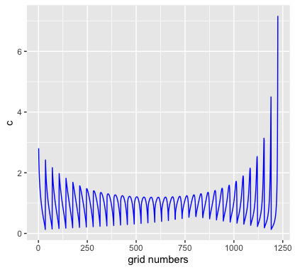
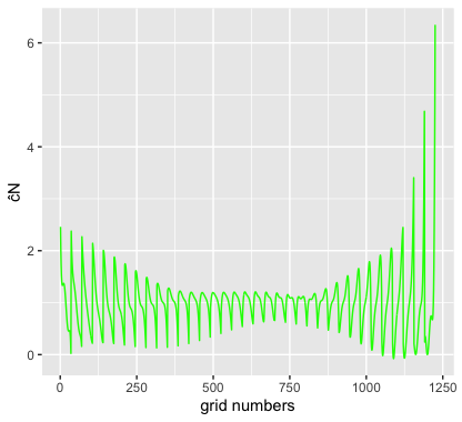
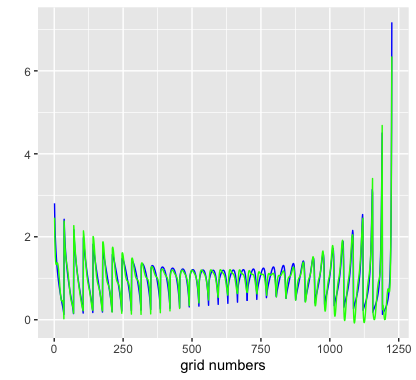
Figure 2: Loss-ALAE. 2-D line plot: Gumbel copula density with parameter $1.45$ (left); $\widehat{c}^{[5]}$ (middle); and their superposition (right).

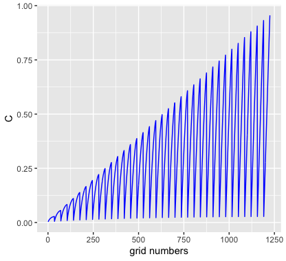
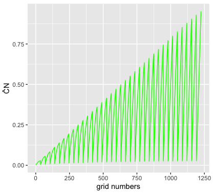
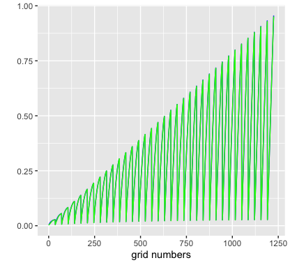
Figure 3: Loss-ALAE. 2-D line plot: Gumbel copula with parameter $1.45$ (left); $\widehat{C}^{[5]}$ (middle); and their superposition (right).

We consider a very classical data set in the copula literature, namely the Loss-ALAE data set, that was collected by the US Insurance Services Office. It contains $1500$ general liability claims each composed of the indemnity payment (Loss) and the allocated loss adjustment expense (ALAE). We excluded $34$ censored observations of the data set. Many authors have used copulas to model the dependence between the two variables in this data set, including Frees and Valdez, (1998), Klugman and Parsa, (1999), Chen and Fan, (2005), Genest et al., (2006), Denuit et al., (2006) and Chen et al., (2010). The general conclusion is that the Gumbel copula provides an adequate fit for these data. Our purpose here is not to take back the analyses, but to confront our own estimator to the adjusted Gumbel copula. Figure 1 (right in the last row) shows the graph of the function LSCV using the selection rule prescribed in section 4.1. The selected truncation parameter is $N=5$. This figure also shows the proximity between our estimator $\widehat{C}^{[5]}$ and the Gumbell copula. To confirm the proximity of the copula as well as its density, we propose to compare them point by point on a grid $\mathcal{G}$ with $36\times 36$ points uniformly chosen on $I^{2}$. The corresponding 1296 values associated to the copula density estimator and to the theoretical Gumbel copula density are represented in Figure 2. The similarities between the two densities are clearly demonstrated, even at the boundaries of $I^{2}$. The same analysis of the copula is displayed in Figure 3. It appears that the Gumbel copula and the estimator copula merge very well. Note that the grid numbers on the x-axis of these figures represent the row number sequence in the data frame $\mathcal{G}$. So each number corresponds to a couple $(u_{j},v_{j})$.

Figure 1 here

Figure 2 here

Figure 3 here

In conclusion, even if (4) is not satisfied for a Gumbel copula density we obtain a very efficient estimators. As explained in Appendix 7 this is due to the fact that for any $\epsilon>0$, writing $c$ the Gumbel copula density, there exists a function $c^{\prime}\in\mathbb{L}^{2}([0,1]^{d})$ such that, for all $\mathbf{u}$, $|c(u)-c^{\prime}(u)|<\epsilon$. Their associated copula coefficients can also be as close as desired. Then our procedure yields a good estimators of $c^{\prime}$ which is also a good approximation of $c$.

5.2 Financial data

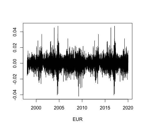
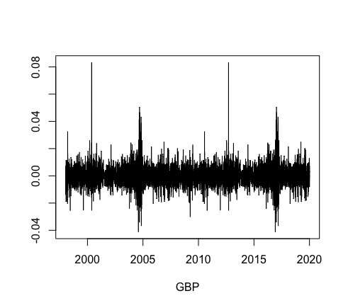
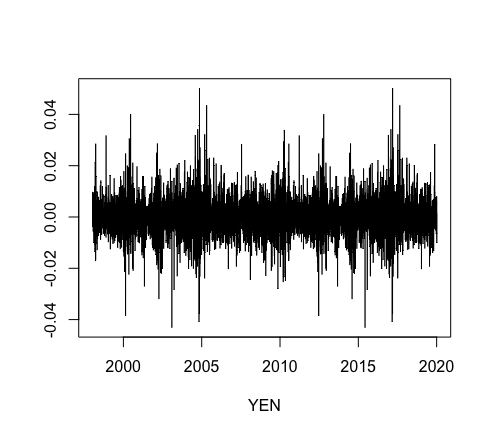
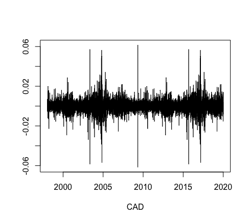
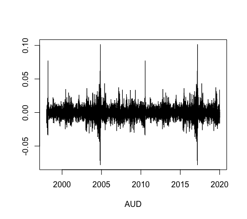
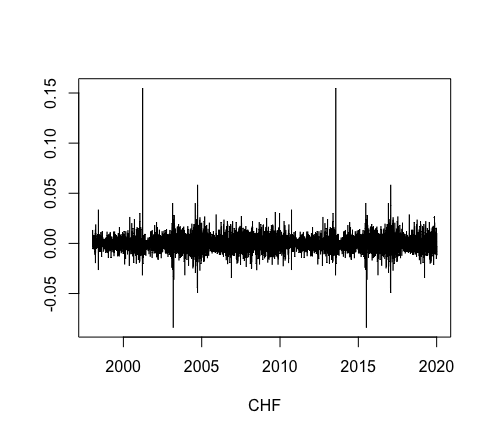
Figure 4: Time plots of daily log returns of Euro, Great British pound, Japanese yen, Canadian Dollar, Australian Dollar and Swiss franc

In this data analysis, we study the dependence structure between the series of the most used exchange rates in foreign exchange markets. Data are available from IMF (International Monetary Fund) rates database and consists in daily currency exchange rates from January $1^{st}$, $1994$ to July $31^{th}$, $2020$ for a total of $5551$ business days (any day except weekends and some holidays). We exclude from our analysis $1049$ observations with at least one missing value. By the standard continuously compounded return formula, we consider the log-returns of six exchanges rates: the Euro (EUR), the Great British pound (GBP), the Japanese yen (YEN), the Canadian dollar (CAD), the Swiss franc (CHF) and the Australian dollar (AUD). The time plots of these returns are shown in Figure 4. These time plots of log returns have a similarly behave with time and show the stylized fact of clustering volatility. We also notice the appearance of extreme values. Summary statistics for these returns are displayed in Table 8. It reveals that the mean and median of log-returns of these six exchange rates are very close to zero. Their distribution are positively skewed (right tailed) and leptokurtic (kurtosis value higher than the kurtosis of normal distribution whose value is three). The CHF has the highlest kurtosis and skewness, the EUR the lowest kurtosis and the CAD the lowest skewness. As it was expected due to more frequent occurrence of extreme values in Figure 4, none of daily log returns passed the Jarque-Bera (JB) test ($P_{value}<0.001$) where the null hypothesis is that the log-return series are normally distributed. As a result, the use of standard models is not appropriate in this context because one of the most important assumptions of several models of the financial time series is the normality of returns.

Tables 10 and 11 give respectively the optimal degree parameters and Kendall’s rank correlations between the six daily log-returns. It shows that the proposed estimators don’t need a high optimal truncation order. The largest degree parameter is $N=16$ (EUR/CHF) and the smallest one is $N=3$ (EUR/YEN). Futher, various Kendall correlations are small values, positive for some pairs of daily log returns and negative for others. The pair EUR/CHF has the highest Kendall correlation in absolute value ($\tau=0.6308960$). We note that a large value for $N$ increases the bias and consequently decreases the asymmetrical structure.

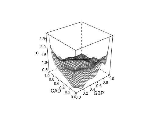
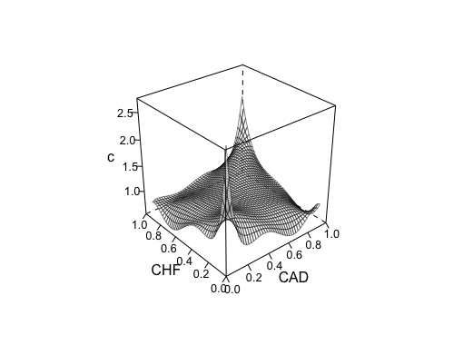
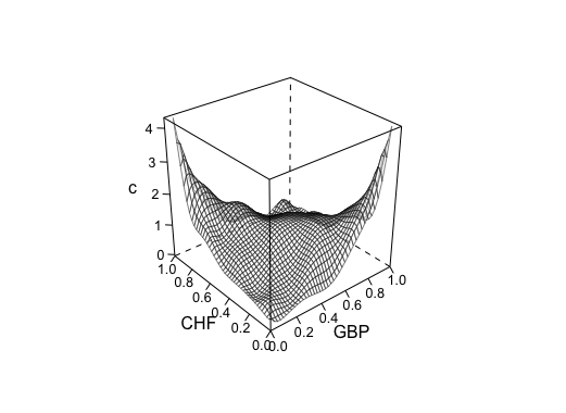
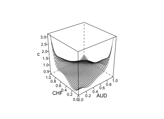
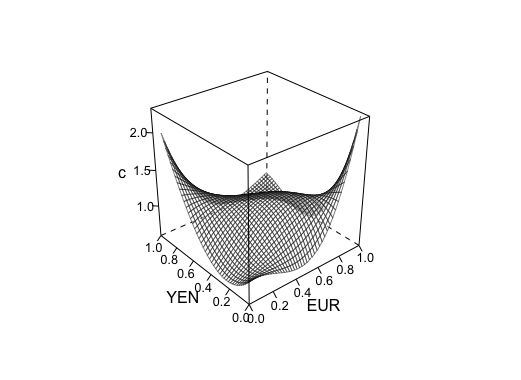
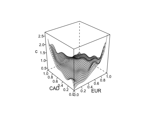
Figure 5: Estimators of the copula density for Canadian Dollar/Great British pound, Swiss franc/Canadian Dollar, Swiss franc/Great British pound, Swiss franc/Australian Dollar, Japanese yen/Euro and Canadian Dollar/Euro

As it was expected from the simulation studies in Section 4, we notice a close link between the Kendall coefficients and the optimal degree parameters of proposed estimators. Both indicators increase or decrease simultaneously. These information are useful for the development of risk diversification strategies since the investment in a portfolio of various assets reduces risk, particularly in exchange rate management. The study can be extended to calculations of the tail value at risk and risk measure expected shortfall. The different pairs daily log return are presented in Figure 5 and 6. We see that the proposed approach captures very well the asymmetry in the dependence structure between these pairs of daily log returns exchange rate.

Table 8 here

Table 10 here

Table 11 here

Figure 4 here

Figure 5 here

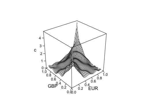
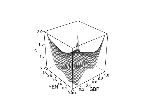
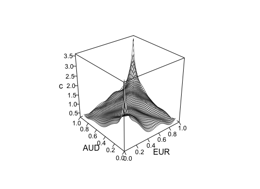
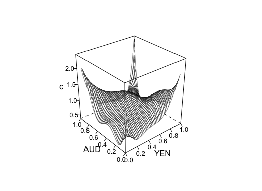
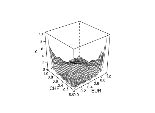
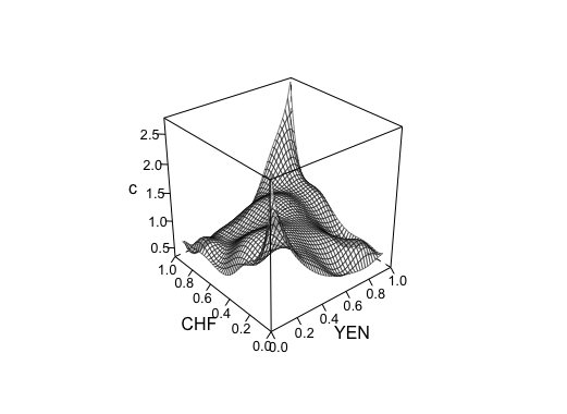
Figure 6: Estimators of the copula density for Euro/Great British pound, Japanese yen/Great British pound, Australian Dollar/Euro, Australian Dollar/Japanese yen, Swiss franc/Euro and Swiss franc/Japanese yen

Figure 6 here

6 Conclusion

In this paper a very simple nonparametric estimator of the copula density based on shifted Legendre polynomials is proposed. A new copula estimator is then deduced based on copula coefficients. Both estimators are easy to implement with an automatic selection of degree approximation. A R program is available on Github-yvesngounou. Various theoretical properties are demonstrated, including asymptotic convergence and optimality in the minimax sense. Experimental results clearly demonstrated the performance of the proposed estimators. The proposed copula estimators seem to outperform all its recent competitors found in the literature according to the MIAE, MISE and MK-SE criterion in various scenarios. These experiment results also showed the superiority of the proposed copula density estimator. These performances could also be improved when considering different orders for $N_{1},N_{2},\cdots,N_{d}$ instead of equal values $N_{1}=\cdots=N_{d}$. This seems possible at a reasonable computationally cost. In the independence case, the estimator is extremely accurate because the correct copula is generally selected. This result may lead to thinking about the construction of an independence test. Moreover, the correspondence that we have shown between the copula coefficients and the Spearman’s rho is an interesting direction for future research. Real situations in actuarial and financial frameworks have demonstrated the adaptability of the proposed method. Finally, this approach by orthogonal projections should also allow us to construct test statistics to compare copulas.

We close this conclusion by recalling that this approach is nonparametric and then hypothesis (4) cannot be verified. However, the method works extremely well even for cases where the density is not square integrable which makes it very useful in practice. We explain this phenomenon in Appendix 7.

APPENDIX: Proofs

We will denote

$$\displaystyle\sup\lvert\widehat{F}_{j}-F_{j}\rvert:=\lVert\widehat{F}_{j}-F_{j}\rVert_{\infty},\quad\pi(\bm{m})=:\displaystyle\prod_{j=1}^{d}m_{j},\quad\max\{N_{j};j:=1,\cdots,d\}:=N_{max}.$$

Let begin with the following useful lemmas

Lemma 1

$$\displaystyle\lVert\widehat{F}_{j}-F_{j}\rVert_{\infty}=o_{\mathbb{P}}(1)\text{ and }\displaystyle\lVert\widehat{F}_{j}-F_{j}\rVert_{\infty}=\mathcal{O}_{\mathbb{P}}(\sqrt{n^{-1}})$$

According to the Massart inequality (Massart, (1990)), we get

$$\displaystyle\forall\epsilon>0,\quad\mathbb{P}\left(\lVert\widehat{F}_{j}-F_{j}\rVert_{\infty}>\epsilon\right)\leq 2e^{-2n\epsilon^{2}}$$ (13)

and the results follow.

Lemma 2

$$\displaystyle\mathbb{E}\lVert\widehat{F}_{j}-F_{j}\rVert_{\infty}^{2}\leq n^{-1}\quad\text{ and }\quad\displaystyle\mathbb{E}\lVert\widehat{F}_{j}-F_{j}\rVert_{\infty}\leq\sqrt{n^{-1}}$$

Denoting $Y:=\lVert\widehat{F}_{j}-F_{j}\rVert_{\infty}$ and using (13), we see that

$$\displaystyle\mathbb{E}(Y)\leq\sqrt{\mathbb{E}(Y^{2})}=\sqrt{\int_{0}^{+\infty}\mathbb{P}(Y>\sqrt{s})ds}\leq\sqrt{\int_{0}^{+\infty}2e^{-2ns^{2}}ds}=\sqrt{n^{-1}}$$

and the results follow.

Lemma 3

For all $\alpha\geq 1$,

$$\displaystyle\sum_{{\mathbf{m}}\leq{\mathbf{N}}}\big{(}\pi(\bm{m})\big{)}^{\alpha}\leq N_{max}^{d(\alpha+1)}$$

We have

$$\displaystyle\sum_{{\mathbf{m}}\leq{\mathbf{N}}}\big{(}\pi(\bm{m})\big{)}^{\alpha}=\prod_{j=1}^{d}\sum_{m_{j}=0}^{N_{j}}m^{\alpha-1}_{j}m_{j}\leq N_{max}^{d(\alpha-1)}\prod_{j=1}^{d}\sum_{m_{j}=0}^{N_{j}}m_{j}\leq N_{max}^{d(\alpha-1)}\prod_{j=1}^{d}\frac{N_{j}(N_{j}+1)}{2}\leq N_{max}^{d(\alpha-1)}\prod_{j=1}^{d}N_{j}^{2}\leq N_{max}^{d(\alpha+1)}.$$

Lemma 4

For all $u\in I$ we have

$$|Q_{m}(u)|\leq\eta_{1}m^{1/2} {\rm and} |Q^{\prime}_{m}(u)|\leq\eta_{2}m^{5/2}\qquad\forall m>0,$$ (14)

where $\eta_{1}=\sqrt{3}$ and $\eta_{2}=2\sqrt{3}$.

See for instance inequalities $22.14$ on page $791$ of Abramowitz and Stegun, (1970) or Boas Jr, (1969). .

Proof of Proposition 1

From (2) we have $h_{\mathbf{U}}=c$. Since $(\mathbf{Q}_{\mathbf{m}})_{\mathbf{m}\in\mathbb{N}^{d}}$ forms a dense orthogonal basis with respect to the uniform measure on $I^{d}$, by (4) we have

$$h_{\mathbf{U}}(u_{1},\cdots,u_{d}) =\displaystyle\sum_{\mathbf{m}\in\mathbb{N}^{d}}\displaystyle\left(\int c(v_{1},\cdots,v_{d})\mathbf{Q}_{\mathbf{m}}(\mathbf{v})dv_{1}\cdots dv_{d}\right)\mathbf{Q}_{\mathbf{m}}(\mathbf{u}),$$

which gives (5), and (6) follows by integration.

6.1 Proof of Proposition 2

Assume that $u_{i}=0$. Then we have

$$\displaystyle\widehat{C}^{[{\mathbf{N}}]}({\mathbf{u}})=\sum_{{\mathbf{m}}\leq{\mathbf{N}}}\widehat{\rho}_{{\mathbf{m}}}\left(\int_{0}^{0}Q_{m_{i}}(x_{i})\mu(dx_{i})\right)\prod_{\begin{subarray}{c}j=1\\ j\neq i\end{subarray}}^{d}\int_{0}^{u_{j}}Q_{m_{j}}(x_{j})\mu(dx_{j})=0,$$

and $i)$ is proved. To prove $ii)$ assume that $\displaystyle\mathbf{u}=(1,\cdots,1,u_{i},1,\cdots,1)$. Then

$$\displaystyle\widehat{C}^{[{\mathbf{N}}]}({\mathbf{u}}) = \sum_{{\mathbf{m}}\leq{\mathbf{N}}}\widehat{\rho}_{{\mathbf{m}}}\left(\int_{0}^{u_{i}}Q_{m_{i}}(x_{i})\mu(dx_{i})\right)\prod_{\begin{subarray}{c}j=1\\ j\neq i\end{subarray}}^{d}\int_{0}^{1}Q_{m_{j}}(x_{j})\mu(dx_{j})$$

$$= \sum_{{\mathbf{m}}\leq{\mathbf{N}}}\widehat{\rho}_{{\mathbf{m}}}\left(\int_{0}^{u_{i}}Q_{m_{i}}(x_{i})\mu(dx_{i})\right)\prod_{\begin{subarray}{c}j=1\\ j\neq i\end{subarray}}^{d}\delta_{0,m_{j}}$$

$$= \widehat{\rho}_{\mathbf{0}}\int_{0}^{u_{i}}Q_{0}(x_{i})\mu(dx_{i})=\int_{0}^{u_{i}}1\;\mu(dx_{i})=u_{i}.$$

$iii)$ is immediate from $\widehat{\rho}_{\mathbf{0}}=1$ and $Q_{0}=1$.

Proof of Proposition 3

By orthogonality of the polynomials we have

$$\displaystyle\int_{I^{d}}\widehat{c}^{[{\mathbf{N}}]}({\mathbf{u}})\mathbf{\mu}(d{\mathbf{u}}) = \sum_{{\mathbf{m}}\leq{\mathbf{N}}}\widehat{\rho}_{{\mathbf{m}}}\prod_{j=1}^{d}\int_{0}^{1}Q_{m_{j}}(u_{j})\mu(du_{j})$$

$$= \sum_{{\mathbf{m}}\leq{\mathbf{N}}}\widehat{\rho}_{{\mathbf{m}}}\prod_{j=1}^{d}\delta_{0,m_{j}}$$

$$= 1$$

which yields $i)$. The proof of $ii)$ is very similar since $\rho_{\mathbf{m}}=0$ if exactly $d-1$ components of $\mathbf{m}$ are null. $iii)$ is immediate.

Proof of Proposition 4

We have

$$\displaystyle\rho_{11} = \mathbb{E}\left(Q_{1}(F_{X_{1}}(X_{1}))Q_{1}(F_{X_{2}}(X_{2}))\right)$$

$$= \mathbb{E}_{C}\left(Q_{1}(U_{1}))Q_{1}(U_{2})\right)$$

$$= \int_{0}^{1}\int_{0}^{1}\left(\sqrt{3}(2u_{1}-1).\sqrt{3}(2u_{2}-1)\right)C(du_{1},du_{2})$$

$$= 3\int_{0}^{1}\int_{0}^{1}\left(4u_{1}u_{2}-2u_{1}-2u_{2}+1\right)C(du_{1},du_{2})$$

$$= 3\left(\int_{0}^{1}\int_{0}^{1}4u_{1}u_{2}dC(u_{1},u_{2})-2(\frac{1}{2})-2(\frac{1}{2})+1\right)$$

$$= 12\int_{0}^{1}\int_{0}^{1}4u_{1}u_{2}dC(u_{1},u_{2})-3$$

$$= \rho_{C}.$$

Proof of Proposition 5

We have

$$\displaystyle\widehat{c}^{[{\mathbf{N}}]}({\mathbf{u}})-\tilde{c}^{[{\mathbf{N}}]}({\mathbf{u}}) = \sum_{{\mathbf{m}}\leq{\mathbf{N}}}(\widehat{\rho}_{{\mathbf{m}}}-\tilde{\rho}_{{\mathbf{m}}}\mathbf{Q}_{\mathbf{m}}({\mathbf{u}}))$$

$$= \displaystyle\sum_{{\mathbf{m}}\leq{\mathbf{N}}}\frac{1}{n}\sum_{i=1}^{n}\Bigg{(}\prod_{j=1}^{d}Q_{m_{j}}(\widehat{F}_{j}(X_{ij}))-\prod_{j=1}^{d}Q_{m_{j}}(F_{j}(X_{ij}))\Bigg{)}\mathbf{Q}_{\mathbf{m}}({\mathbf{u}}).$$

By Taylor expansion, we obtain

$$|\prod_{j=1}^{d}Q_{m_{j}}(\widehat{F}_{j}(X_{ij}))-\prod_{j=1}^{d}Q_{m_{j}}(F_{j}(X_{ij}))| \leq \sum_{j=1}^{d}\eta_{2}m_{j}^{5/2}\displaystyle\prod_{i\neq j}\eta_{1}m_{i}^{1/2}\|\widehat{F}_{j}-F_{j}\|_{\infty}$$ (15)

$$\leq M({\mathbf{m}})\sum_{j=1}^{d}\|\widehat{F}_{j}-F_{j}\|_{\infty},$$

where $M({\mathbf{m}})=\eta_{2}\eta_{1}^{d-1}\pi({\mathbf{m}})^{1/2}\max(m_{j})^{2}$. It follows that

$$\displaystyle|\widehat{c}^{[{\mathbf{N}}]}({\mathbf{u}})-\tilde{c}^{[{\mathbf{N}}]}({\mathbf{u}})| \leq \displaystyle\sum_{{\mathbf{m}}\leq{\mathbf{N}}}M({\mathbf{m}})\max|\mathbf{Q}_{{\mathbf{m}}}|\sum_{j=1}^{d}\|\widehat{F}_{j}-F_{j}\|_{\infty}$$ (16)

$$\leq \displaystyle\eta_{2}\eta_{1}^{2d-1}N_{max}^{2}\sum_{{\mathbf{m}}\leq{\mathbf{N}}}\pi({\mathbf{m}})\sum_{j=1}^{d}\|\widehat{F}_{j}-F_{j}\|_{\infty}$$

$$\leq \eta_{2}\eta_{1}^{2d-1}N_{max}^{2d+2}\sum_{j=1}^{d}\|\widehat{F}_{j}-F_{j}\|_{\infty},$$

from Lemma 3, which yields $i)$ since $\|\widehat{F}_{j}-F_{j}\|_{\infty}=\mathcal{O}_{\mathbb{P}}\big{(}\sqrt{n^{-1}}\big{)}$ according to Lemma 1.
We obtain $ii)$ analogously.

Proof of Proposition 6.

By orthogonality of the Legendre polynomials we have

$$\|\widehat{c}^{[\mathbf{N}]}-c\|_{2}^{2} = \sum_{{\mathbf{m}}\leq{\mathbf{N}}}\left(\widehat{\rho}_{{\mathbf{m}}}-\rho_{{\mathbf{m}}}\right)^{2}+\sum_{{\mathbf{m}}\not\leq{\mathbf{N}}}\rho_{{\mathbf{m}}}^{2},$$

which gives result.

Proof of Corollary 1

By orthogonality, we have

$$MISE(\widehat{c}^{[\mathbf{N}]})-MISE(\tilde{c}^{[\mathbf{N}]}) = \mathbb{E}\left(\sum_{\mathbf{m}\leq\mathbf{N}}(\widehat{\rho}_{\mathbf{m}}-\rho_{\mathbf{m}})^{2}\right)-\mathbb{E}\left(\sum_{\mathbf{m}\leq\mathbf{N}}(\tilde{\rho}_{\mathbf{m}}-\rho_{\mathbf{m}})^{2}\right)$$ (17)

$$= \mathbb{E}\sum_{\mathbf{m}\leq\mathbf{N}}(\widehat{\rho}_{\mathbf{m}}-\tilde{\rho}_{\mathbf{m}})\left((\widehat{\rho}_{\mathbf{m}}-\tilde{\rho}_{\mathbf{m}})+2(\tilde{\rho}_{\mathbf{m}}-\rho_{\mathbf{m}})\right).$$

From (15), we first have

$$|\widehat{\rho}_{\mathbf{m}}-\tilde{\rho}_{\mathbf{m}}| \leq M({\mathbf{m}})\sum_{j=1}^{d}\|\widehat{F}_{j}-F_{j}\|_{\infty},$$

and since

$$\|\widehat{F}_{j}-F_{j}\|_{\infty}=\mathcal{O}_{\mathbb{P}}\big{(}\sqrt{n^{-1}}\big{)}$$

it follows that

$$\widehat{\rho}_{\mathbf{m}}-\tilde{\rho}_{\mathbf{m}}=\mathcal{O}_{\mathbb{P}}(\sqrt{n^{-1}}).$$ (18)

Furthermore, by the Central Limit Theorem we have

$$\sqrt{n}\left(\tilde{\rho}_{\mathbf{m}}-\rho_{\mathbf{m}}\right)\xrightarrow{\enskip\mathcal{L}\enskip}\mathcal{N}\left(0,\mathbb{V}\big{(}\prod_{j=1}^{d}Q_{m_{j}}(F_{j}(X_{ij})\big{)}\right),$$

where $\displaystyle\mathbb{V}\big{(}\prod_{j=1}^{d}Q_{m_{j}}(F_{j}(X_{ij})\big{)}<\infty$ since $\bm{N}$ is fixed and independent of $n$. Then

$$\tilde{\rho}_{\mathbf{m}}-\rho_{\mathbf{m}} = \mathcal{O}_{\mathbb{P}}\big{(}\sqrt{n^{-1}}\big{)}.$$ (19)

Combining (17), (15) and (19) we get

$$MISE(\widehat{c}^{[\mathbf{N}]})=MISE(\tilde{c}^{[\mathbf{N}]})+\mathcal{O}\big{(}n^{-1}\big{)}.$$

Proof of Corollary 2

From Proposition 6, we have

$$\mathbb{E}\left(\|\widehat{c}^{[\mathbf{N}]}-c\|_{2}^{2}\right)=\mathbb{E}\left(\sum_{\mathbf{m}\leq\mathbf{N}}(\widehat{\rho}_{\mathbf{m}}-\rho_{\mathbf{m}})^{2}\right)+\displaystyle\sum_{\mathbf{m}\not\leq\mathbf{N}}\rho_{\mathbf{m}}^{2}.$$

From the elementary inequality $\displaystyle 2ab\leq a^{2}+b^{2}$ for any $a,b\in\mathbb{R}$, we get

$$\mathbb{E}\left(\|\widehat{c}^{[\mathbf{N}]}-c\|_{2}^{2}\right) \leq 2\mathbb{E}\left(\sum_{\mathbf{m}\leq\mathbf{N}}(\widehat{\rho}_{\mathbf{m}}-\tilde{\rho}_{\mathbf{m}})^{2}\right)+2\mathbb{E}\left(\sum_{\mathbf{m}\leq\mathbf{N}}(\tilde{\rho}_{\mathbf{m}}-\rho_{\mathbf{m}})^{2}\right)+\displaystyle\sum_{\mathbf{m}\not\leq\mathbf{N}}\rho_{\mathbf{m}}^{2}$$ (20)

$$:= 2A_{1}+2A_{2}+A_{3}.$$

Clearly, $A_{3}\rightarrow 0$, as $N\rightarrow\infty$ as a tail of a convergent series.

Moreover by (14) we have

$$A_{2} =\sum_{\mathbf{m}\leq\mathbf{N}}\frac{1}{n}\mathbb{V}(\displaystyle\prod_{j=1}^{d}Q_{m_{j}}(F_{j}(X_{j})))$$

$$\leq\sum_{\mathbf{m}\leq\mathbf{N}}\displaystyle\frac{1}{n}\eta_{1}^{2d}\displaystyle\prod_{j=1}^{d}m_{j}$$

$$\leq\displaystyle\frac{\eta_{1}^{2d}N_{max}^{2d}}{n},$$ (21)

By (H) $A_{2}\rightarrow 0$ as $n\rightarrow\infty$. To conclude, we combine (15) with (14) to obtain

$$A_{1} =\sum_{\mathbf{m}\leq\mathbf{N}}\displaystyle\frac{1}{n^{2}}\displaystyle\sum_{i=1}^{n}\displaystyle\sum_{i^{\prime}=1}^{n}\mathbb{E}\Bigg{[}\Bigg{(}\prod_{j=1}^{d}Q_{m_{j}}(\widehat{F}_{j}(X_{ij}))-\prod_{j=1}^{d}Q_{m_{j}}(F_{j}(X_{ij}))\Bigg{)}$$

$$\ \ \ \ \ \ \ \ \ \ \times\Bigg{(}\prod_{j=1}^{d}Q_{m_{j}}(\widehat{F}_{j}(X_{i^{\prime}j}))-\prod_{j=1}^{d}Q_{m_{j}}(F_{j}(X_{i^{\prime}j})))\Bigg{)}\Bigg{]}$$

$$\leq\sum_{\mathbf{m}\leq\mathbf{N}}\displaystyle\frac{1}{n^{2}}\displaystyle\sum_{i=1}^{n}\displaystyle\sum_{i^{\prime}=1}^{n}\mathbb{E}\Bigg{(}M({\mathbf{m}})^{2}\left(\sum_{j=1}^{d}\|\widehat{F}_{j}-F_{j}\|_{\infty}\right)^{2}\Bigg{)}$$

$$\leq d\sum_{\mathbf{m}\leq\mathbf{N}}M({\mathbf{m}})^{2}\sum_{j=1}^{d}\mathbb{E}\left(\|\widehat{F}_{j}-F_{j}\|^{2}_{\infty}\right),$$

according to Hölder’s sum inequality.

Since $M({\mathbf{m}})=\eta_{1}^{d-1}\eta_{2}\pi({\mathbf{m}})^{1/2}\max(m_{j})^{2}$ and $\mathbb{E}\left(\|\widehat{F}_{j}-F_{j}\|^{2}_{\infty}\right)\leq n^{-1}$, we see from to Lemma 2 that there exists a constant $\eta>0$ such that

$$A_{1} \leq\frac{d^{2}\eta_{1}^{2d-2}\eta^{2}_{2}}{n}\sum_{\mathbf{m}\leq\mathbf{N}}\pi(\bm{m})\max(m_{j})^{4}$$

$$\leq\frac{d^{2}\eta_{1}^{2d-2}\eta^{2}_{2}N_{max}^{4}}{n}\sum_{\mathbf{m}\leq\mathbf{N}}\pi(\bm{m})$$

$$\leq\frac{d^{2}\eta_{1}^{2d-2}\eta^{2}_{2}N_{max}^{2d+4}}{n},$$ (22)

and then $A_{1}\rightarrow 0$ as $n\rightarrow\infty$.

Proof of Proposition 7

We have

$$\displaystyle\mathbb{E}\left(\widehat{c}^{[{\mathbf{N}}]}({\mathbf{u}})\right)=\mathbb{E}\left(\tilde{c}^{[{\mathbf{N}}]}({\mathbf{u}})\right)+\displaystyle\mathbb{E}\left(\widehat{c}^{[{\mathbf{N}}]}({\mathbf{u}})-\mathbb{E}\tilde{c}^{[{\mathbf{N}}]}({\mathbf{u}})\right).$$

Since $\mathbb{E}\left(\tilde{\rho}_{{\mathbf{m}}}\right)=\rho_{{\mathbf{m}}}$, we have

$$\displaystyle\mathbb{E}\left(\tilde{c}^{[{\mathbf{N}}]}(\mathbf{u})\right) = \sum_{{\mathbf{m}}\leq{\mathbf{N}}}\mathbb{E}\left(\tilde{\rho}_{{\mathbf{m}}}\right)\prod_{j=1}^{d}Q_{m_{j}}(u_{j})=\sum_{{\mathbf{m}}\leq{\mathbf{N}}}\rho_{{\mathbf{m}}}\prod_{j=1}^{d}Q_{m_{j}}(u_{j}),$$

which tends to $c\left(\mathbf{u}\right)$ as $n$ tends to $\infty$. From (16), according to Lemma 2, we have

$$\displaystyle|\mathbb{E}\widehat{c}^{[{\mathbf{N}}]}({\mathbf{u}})-\mathbb{E}\tilde{c}^{[{\mathbf{N}}]}({\mathbf{u}})| \leq \displaystyle\eta_{2}\eta_{1}^{2d-1}N_{max}^{2d+2}\sum_{j=1}^{d}\mathbb{E}\|\widehat{F}_{j}-F_{j}\|_{\infty}$$

$$\leq d\displaystyle\eta_{2}\eta_{1}^{2d-1}\frac{N_{max}^{2d+2}}{\sqrt{n}}.$$

Under assumption $(\bm{H})$, we deduce that

$$\displaystyle\mathbb{E}\left(\widehat{c}^{[{\mathbf{N}}]}(\mathbf{u})\right)\longrightarrow c(\mathbf{u})\text{ as }n\to\infty.$$

and analogously

$$\displaystyle\mathbb{E}\left(\widehat{C}^{[{\mathbf{N}}]}(\mathbf{u})\right)\longrightarrow C(\mathbf{u})\text{ as }n\to\infty.$$

Proof of Proposition 8

Combining (20) with (21)- (22) yields

$$\displaystyle\mathbb{E}(\|\widehat{c}^{[{\mathbf{N}}]}-c\|_{2}^{2}) \leq \displaystyle 2\frac{d^{2}\eta_{1}^{2d-2}\eta^{2}_{2}N_{max}^{2d+4}}{n}+2\displaystyle\frac{\eta_{1}^{2d}N_{max}^{2d}}{n}+\displaystyle\sum_{\mathbf{m}\not\leq\mathbf{N}}\rho_{\mathbf{m}}^{2}$$

$$= \big{(}2d^{2}\eta_{1}^{2d-2}\eta^{2}_{2}+2\displaystyle\frac{\eta_{1}^{2d}}{N_{max}^{4}}\big{)}\displaystyle\frac{N_{max}^{2d+4}}{n}+\displaystyle\sum_{\mathbf{m}\not\leq\mathbf{N}}\rho_{\mathbf{m}}^{2}$$

$$\leq \displaystyle\frac{\eta N_{max}^{2d+4}}{n}+\displaystyle\sum_{\mathbf{m}\not\leq\mathbf{N}}\rho_{\mathbf{m}}^{2}\left(1+\sum_{i=1}^{d}m_{i}^{\beta_{i}}\right)\left(1+\sum_{i=1}^{d}m_{i}^{\beta_{i}}\right)^{-1},$$

with $\eta=2d^{2}\eta_{1}^{2d-2}\eta_{2}^{2}+{2\eta_{1}^{2d}}$.

Observe that we can decompose

$$\left\{\bm{m}\in\mathbb{N}^{d}\,/\,\bm{m}\not\leq\bm{N}\right\}=\bigcup\limits_{j=1}^{d}\left\{\bm{m}\in\mathbb{N}^{d}/m_{j}>N_{j}{\rm\ and\ }\mathbf{m}_{j+}\leq\bm{N}_{j+}\right\},$$

where $\mathbf{m}_{j+}=(m_{j+1},\cdots,m_{d})$ and $\mathbf{N}_{j+}=(N_{j+1},\cdots,N_{d})$, with the convention $\mathbf{m}_{d+}=\mathbf{N}_{d+}=\varnothing$. We also write $\mathbf{m}_{j-}=(m_{1},\cdots,m_{j-1})$ and $\mathbf{N}_{j-}=(N_{1},\cdots,N_{j-1})$, with the convention $\mathbf{m}_{1-}=\mathbf{N}_{1-}=\varnothing$. We use this decomposition as follows:

$$\displaystyle\mathbb{E}(\|\widehat{c}^{[{\mathbf{N}}]}-c\|_{2}^{2}) \leq \displaystyle\frac{\eta N_{max}^{2d+4}}{n}+\displaystyle\sum_{j=1}^{d}\sum_{m_{j}>N_{j}}\sum_{\begin{array}[]{l}\tiny\mathbf{m}_{j-}\in\mathbb{N}^{j-1},\\ \tiny\mathbf{m}_{j+}\leq\bm{N}_{j+}\end{array}}\rho_{\mathbf{m}}^{2}\left(1+\sum_{i=1}^{d}m_{i}^{\beta_{i}}\right)\left(1+\sum_{i=1}^{d}m_{i}^{\beta_{i}}\right)^{-1}$$

$$\leq \displaystyle\frac{\eta N_{max}^{2d+4}}{n}+\displaystyle\sum_{j=1}^{d}\sum_{m_{j}>N_{j}}\sum_{\begin{array}[]{l}\tiny\mathbf{m}_{j-}\in\mathbb{N}^{j-1},\\ \tiny\mathbf{m}_{j+}\leq\bm{N}_{j+}\end{array}}\rho_{\mathbf{m}}^{2}\left(1+\sum_{i=1}^{d}m_{i}^{\beta_{i}}\right)m_{j}^{-\beta_{j}},$$

since for all $j=1,\cdots,d,$

$$\left(1+\sum_{i=1}^{d}m_{i}^{\beta_{i}}\right)^{-1} \leq m_{j}^{-\beta_{j}}.$$

Observe also that

$$b=\left(\sum_{j=1}^{d}\beta_{j}^{-1}\right)^{-1}\leq\beta_{j},\text{ for all }j=1,\cdots,d.$$

Hence

$$\displaystyle\mathbb{E}(\|\widehat{c}^{[{\mathbf{N}}]}-c\|_{2}^{2}) \leq \displaystyle\frac{\eta N_{max}^{2d+4}}{n}+\displaystyle\sum_{j=1}^{d}\sum_{m_{j}>N_{j}}N_{j}^{-\beta_{j}}\sum_{\begin{array}[]{l}\tiny\mathbf{m}_{j-}\in\mathbb{N}^{j-1},\\ \tiny\mathbf{m}_{j+}\leq\bm{N}_{j+}\end{array}}\rho_{\mathbf{m}}^{2}\left(1+\sum_{i=1}^{d}m_{i}^{\beta_{i}}\right)$$

$$\leq \displaystyle\frac{\eta N_{max}^{2d+4}}{n}+\displaystyle dN_{max}^{-b}\sum_{\mathbf{N}\in\mathbb{N}^{d}}\rho_{\mathbf{m}}^{2}\left(1+\sum_{i=1}^{d}m_{i}^{\beta_{i}}\right)$$

$$\leq \displaystyle\frac{\eta N_{max}^{2d+4}}{n}+LdN_{max}^{-b}.$$ (27)

Since $N_{max}=[n^{\frac{1}{2d+b+4}}]$, we get

$$\mathbb{E}(\|\widehat{c}^{[{\mathbf{N}}]}-c\|_{2}^{2}) \leq \displaystyle(\eta+Ld)n^{\frac{-b}{b+2d+4}}$$

which gives the result.

Proof of Proposition 9.

According to (27) we have

$$\displaystyle\mathbb{E}(\|\widehat{c}^{[{\mathbf{N}}]}-c\|_{2}^{2}) \leq \displaystyle\frac{\eta N_{max}^{2d+4}}{n}+LdN_{max}^{-b},$$

and it follows that

$$\sup_{\displaystyle c\in{\mathcal{F}}_{\bm{\beta}}(L)}\displaystyle\mathbb{E}(\|\widehat{c}^{[{\mathbf{N}}]}-c\|_{2}^{2}) \leq \displaystyle\frac{\eta N_{max}^{2d+4}}{n}+LdN_{max}^{-b}.$$

Since this inequality is satisfied for all $\mathbf{N}\neq\mathbf{0}$ we obtain

$$\displaystyle\mathcal{R}^{\star}(\mathcal{F}_{\bm{\beta}}(L)) \leq \displaystyle\frac{\eta N_{max}^{2d+4}}{n}+LdN_{max}^{-b},$$

where the left hand side does not depend of $\mathbf{N}$. By minimizing the right hand side, we obtain a minimum for $\displaystyle N_{max}=n^{\frac{1}{2d+b+4}}\left(\frac{Lbd}{\eta(2d+4)}\right)^{\frac{1}{2d+b+4}}$ and we conclude that

$$\displaystyle\mathcal{R}^{\star}(\mathcal{F}_{\bm{\beta}}(L))\leq Kv_{n},\text{ where }K=\frac{Ld(2d+b+4)}{2d+4}\left(\frac{Lbd}{\eta(2d+4)}\right)^{\frac{-b}{2d+b+4}}.$$

6.2 Proof of Proposition 10

We have

$$\displaystyle\widehat{LSCV}({\mathbf{N}})= \displaystyle\int_{I^{d}}\left(\widehat{c}^{[{\mathbf{N}}]}({\mathbf{u}})\right)^{2}d{\mathbf{u}}-\displaystyle\frac{2}{n}\displaystyle\sum_{i=1}^{m}\widehat{c}^{[{\mathbf{N}}]}_{-i}\left(\widehat{F}_{1}(X_{i1}),\cdots,\widehat{F}_{d}(X_{id})\right)$$

$$=\sum_{{\mathbf{m}}\leq{\mathbf{N}}}\widehat{\rho}_{{\mathbf{m}}}^{2}-\displaystyle\frac{2}{n}\sum_{i=1}^{n}\sum_{{\mathbf{m}}\leq{\mathbf{N}}}\widehat{\rho}_{{\mathbf{m}}}^{(-i)}\prod_{j=1}^{d}Q_{m_{j}}\Big{(}\widehat{F}_{j}(X_{ij})\Big{)}$$

$$=\sum_{{\mathbf{m}}\leq{\mathbf{N}}}\left(\frac{1}{n}\displaystyle\sum_{i=1}^{n}\prod_{j=1}^{d}Q_{m_{j}}\Big{(}\widehat{F}_{j}(X_{ij})\Big{)}\right)^{2}$$

$$-\frac{2}{n}\sum_{i=1}^{n}\left(\sum_{{\mathbf{m}}\leq{\mathbf{N}}}\left(\frac{1}{n-1}\sum_{\begin{subarray}{c}k=1,\\ k\not\neq i\end{subarray}}^{n}\prod_{j=1}^{d}Q_{m_{j}}\Big{(}\widehat{F}_{j}(X_{kj})\Big{)}\right)\prod_{j=1}^{d}Q_{m_{j}}\Big{(}\widehat{F}_{j}(X_{ij})\Big{)}\right)$$

$$=\frac{1}{n^{2}}\sum_{{\mathbf{m}}\leq N}\left(\displaystyle\sum_{i=1}^{n}\prod_{j=1}^{d}Q_{m_{j}}^{2}\Big{(}\widehat{F}_{j}(X_{ij})\Big{)}+\sum_{\begin{subarray}{c}k\not\neq i\end{subarray}}\prod_{j=1}^{d}Q_{m_{j}}\Big{(}\widehat{F}_{j}(X_{kj})\Big{)}Q_{m_{j}}\Big{(}\widehat{F}_{j}(X_{ij})\Big{)}\right)$$

$$-\frac{2}{n(n-1)}\sum_{{\mathbf{m}}\leq{\mathbf{N}}}\sum_{\begin{subarray}{c}k\not\neq i\end{subarray}}\prod_{j=1}^{d}Q_{m_{j}}\Big{(}\widehat{F}_{j}(X_{kj})\Big{)}Q_{m_{j}}\Big{(}\widehat{F}_{j}(X_{ij})\Big{)}$$

$$=\displaystyle\frac{1}{n^{2}}\sum_{{\mathbf{m}}\leq N}\left(\displaystyle\sum_{i=1}^{n}\prod_{j=1}^{d}Q_{m_{j}}^{2}\Big{(}\widehat{F}_{j}(X_{ij})\Big{)}-\displaystyle\frac{n+1}{n-1}\sum_{k\neq i}\prod_{j=1}^{d}Q_{m_{j}}\Big{(}\widehat{F}_{j}(X_{ij})\Big{)}Q_{m_{j}}\Big{(}\widehat{F}_{j}(X_{kj})\Big{)}\right)$$

6.3 Proof of Proposition 11

If the margins are known, we have

$$\mathbb{E}\left(LSCV(N)\right)=\mathbb{E}\left(\displaystyle\int_{I^{d}}\left(\tilde{c}^{[{\mathbf{N}}]}({\mathbf{u}})\right)^{2}\mu(d{\mathbf{u}})\right)-\displaystyle 2\mathbb{E}\left(\displaystyle\frac{1}{n}\sum_{i=1}^{n}\tilde{c}^{[{\mathbf{N}}]}_{-i}\left(F_{1}(X_{i1}),\cdots,F_{d}(X_{id})\right)\right).$$

In addition we have

$$\displaystyle\mathbb{E}\left(\frac{1}{n}\sum_{i=1}^{n}\tilde{c}^{[{\mathbf{N}}]}_{-i}\left(F_{1}(X_{i1}),\cdots,F_{d}(X_{id})\right)\right)=\displaystyle\frac{1}{n}\sum_{i=1}^{n}\sum_{m\leq N}\mathbb{E}\left(\tilde{\rho}_{m}\right)\mathbb{E}\left(\prod_{j=1}^{d}Q_{m_{j}}(F_{j}(X_{ij}))\right)$$

$$= \sum_{m\leq N}\mathbb{E}(\tilde{\rho}_{m})\int_{\mathbb{R}^{d}}\prod_{j=1}^{d}Q_{m_{j}}(F_{j}(x_{ij}))f(x_{1},\cdots,x_{d})\mu(\mathrm{d}{\mathbf{x}})$$

$$= \sum_{n\leq N}\mathbb{E}(\tilde{\rho}_{n})\int_{I^{d}}\prod_{j=1}^{d}Q_{m_{j}}(u_{j})c\left(u_{1},\cdots,u_{d})\right)\mu(\mathrm{d}{\mathbf{u}})$$

$$= \mathbb{E}\int_{I^{d}}\sum_{m\leq N}\tilde{\rho}_{m}\prod_{j=1}^{d}Q_{m_{j}}(u_{j})c(u_{1},\cdots,u_{d})\mu(\mathrm{d}{\mathbf{u}})$$

$$= \mathbb{E}\int_{I^{d}}\tilde{c}^{[{\mathbf{N}}]}({\mathbf{u}})c({\mathbf{u}})\mu(\mathrm{d}{\mathbf{u}})$$

which implies that

$$\mathbb{E}\left(LSCV(N)\right) = \mathbb{E}\left(\displaystyle\int_{I^{d}}\left(\tilde{c}^{[{\mathbf{N}}]}({\mathbf{u}})\right)^{2}\mu(\mathrm{d}{\mathbf{u}})-2\int_{I^{d}}\tilde{c}^{[{\mathbf{N}}]}({\mathbf{u}})c({\mathbf{u}})\mu(\mathrm{d}{\mathbf{u}})\right)$$

$$= \mathbb{E}\left(\int_{I^{d}}\left(\tilde{c}^{[{\mathbf{N}}]}({\mathbf{u}})-c({\mathbf{u}})\right)^{2}\mu(\mathrm{d}{\mathbf{u}})\right)-\int_{I^{d}}(c({\mathbf{u}}))^{2}\mu(\mathrm{d}{\mathbf{u}}),$$

and we obtain

$$\mathbb{E}\left(LSCV(N)\right) = \mathbb{E}\|\tilde{c}^{[{\mathbf{N}}]}-c\|_{2}^{2}-\|c\|_{2}^{2}.$$ (28)

If the margins are unknown, we combine Corollary 1 and equation (28) to obtain the result.

7 Modifying the copula density to be square integrable

If assumption (4) is not satisfied, one can modify the copula density $c$ with a shrinkage function, writing

$$c(\bm{\theta},\mathbf{u}) = s(\bm{\theta},\mathbf{u})c(\mathbf{u}),$$

for some $\bm{\theta}=(\theta_{1},\cdots,\theta_{p})$. For instance, $s$ can be an exponential tilting defined as follows

$$s(\bm{\theta},\mathbf{u})=\exp\left(-\displaystyle\sum_{j=1}^{p}\displaystyle\frac{\theta_{j}}{u_{j}}\right):=\displaystyle\prod_{j=1}^{d}s_{j}(\theta_{j},u_{j}),$$

with   $\theta_{j}>0$. In that case we obtain

$$c(\bm{\theta},\mathbf{u}) =\displaystyle\sum_{\mathbf{m}\in\mathbb{N}^{p}}\rho_{\bm{\theta},\mathbf{m}}\mathbf{Q}_{\mathbf{m}}({\mathbf{u}})),$$

where

$$\rho_{\bm{\theta},\mathbf{m}} =\mathbb{E}\left(\prod_{j=1}^{d}s_{j}(\theta_{j},U_{j})Q_{m_{j}}(U_{j})\right).$$

We then modify our estimators as follows

$$\widehat{\rho}_{\bm{\theta},\mathbf{j}} =\displaystyle\frac{1}{n}\displaystyle\sum_{i=1}^{n}\left(\prod_{j=1}^{d}s_{j}(\theta_{j},\widehat{U}_{i,j})Q_{m_{j}}(\widehat{U}_{i,j})\right)$$ (29)

and we get a $\mathbf{N}$-th order estimator of $c(\bm{\theta},\mathbf{u})$ as

$$\displaystyle\widehat{c}^{[{\mathbf{N}}]}(\bm{\theta},\mathbf{u}) = \sum_{{\mathbf{m}}\leq{\mathbf{N}}}\widehat{\rho}_{\bm{\theta},{\mathbf{m}}}\prod_{j=1}^{d}Q_{m_{j}}(u_{j}).$$

Clearly the positive functions $c(\bm{\theta},.)$ do not satisfy the properties of copula densities but we expect that the transformation made them square integrable. It gives a way to rewrite the main results of the paper. Since we apply a known transformation we can find an estimation of $c(.)$ thanks to that of $c(\bm{\theta},.)$. More precisely we use

$$\widehat{c}^{[\mathbf{N}]}(\mathbf{u}) = \displaystyle s^{-1}(\mathbf{\theta},\mathbf{u})\widehat{c}^{[\mathbf{N}]}(\bm{\theta},\mathbf{u}).$$

The fact that all factors $\displaystyle s_{j}(\mathbf{\theta}_{j},U_{j})$ and $\displaystyle s_{j}(\mathbf{\theta}_{j},\widehat{U}_{j})$ are bounded is essential here to generalize our methodology and to get the same asymptotic results.

We illustrate this shrinking approach through the bivariate Clayton and Gumbel copulas as follows.

The bivariate Clayton copula.

Its copula density is given by

$$c(u_{1},u_{2}) = (\beta+1)(u_{1}u_{2})^{-(\beta+1)}\big{(}u_{1}^{-\beta}+u_{2}^{-\beta}-1\big{)}^{-(2\beta+1)/\beta},$$

with $u_{1},u_{2}\in(0,1)$ and for $\beta>0$. We choose

$$s(\bm{\theta},\mathbf{u})=\exp\left(-\displaystyle\frac{\theta_{1}}{u_{1}}-\displaystyle\frac{\theta_{2}}{u_{2}}\right),$$

and an easy computation shows that

$$\displaystyle\int_{0}^{1}\displaystyle\int_{0}^{1}\left(s(\bm{\theta},\mathbf{u})c(u_{1},u_{2})\right)^{2}du_{1}du_{2} \leq (\beta+1)\displaystyle\int_{0}^{1}\displaystyle\int_{0}^{1}\exp\left(-\displaystyle\frac{2\theta_{1}}{u_{1}}-\displaystyle\frac{2\theta_{2}}{u_{2}}\right)(u_{1}u_{2})^{-2(\beta+1)}du_{1}du_{2}$$

$$= \displaystyle\int_{1}^{\infty}\displaystyle\int_{1}^{\infty}\exp\left(-{2{\theta_{1}}x}-{2\theta_{2}y}\right)(xy)^{2\beta}dxdy$$

$$<\infty {\rm\ \ for\ all\ }\theta_{1}>0,\theta_{2}>0.$$

The bivariate Gumbel copula.

Its density is given by

$$c(u_{1},u_{2}) = \displaystyle\frac{C(u_{1},u_{2})}{u_{1}u_{2}}\left(\ell_{\beta}(u_{1})+\ell_{\beta}(u_{2})\right)^{-2+2/\beta}\ell_{\beta-1}(u_{1})\ell_{\beta-1}(u_{2})\left(1+(\beta-1)\big{(}\ell_{\beta}(u_{1})+\ell_{\beta}(u_{2})\big{)}^{-1/\beta}\right)$$

where

$$C(u_{1},u_{2})=\exp\left(-\big{(}\ell_{\beta}(u_{1})+\ell_{\beta}(u_{2})\big{)}^{1/\beta}\right) {\rm and} \ell_{\beta}(u)=\big{(}-\log(u)\big{)}^{\beta},$$

with $u_{1},u_{2}\in(0,1)$ and $\beta\geq 1$. We can chek that

$$\displaystyle\int_{0}^{1}\displaystyle\int_{0}^{1}\left(u_{1}^{\theta_{1}}u_{2}^{\theta_{2}}c(u_{1},u_{2})\right)^{2}du_{1}du_{2} < \infty{\rm\ \ for\ all\ }\theta_{1}>0,\theta_{2}>0.$$

In that case the shrinkage factor can be simply $s(\bm{\theta},\mathbf{u})=u_{1}^{\theta_{1}}u_{2}^{\theta_{2}}$.

In conclusion, since $s(\bm{\theta},\mathbf{u})$ is known we can choose arbitrary $\bm{\theta}$ such that for a given small $\epsilon>0$ we have

$$1-\epsilon\leq\displaystyle\frac{c(\bm{\theta},\mathbf{u})}{c(\mathbf{u})}:=s(\bm{\theta},\mathbf{u})<1.$$

The proximity between $c(.)$ and $c(\bm{\theta},)$ explains the very good behavior of the method even for the case where (4) is not satisfied. In that case the coefficient estimators $\widehat{\rho}_{\mathbf{j}}$ and $\widehat{\rho}_{\bm{\theta},\mathbf{j}}$ are very close and so are the density estimators $\widehat{c}^{[\mathbf{N}]}(.)$ and $\widehat{c}^{[\mathbf{N}]}(\bm{\theta},)$

We illustrate numerically this remark in the six sample case for the Clayton and Gumbel copulas, using a tilting exponential factor $s(\bm{\theta},\mathbf{u})=\exp\left(-\displaystyle\frac{\theta_{1}}{u_{1}}-\displaystyle\frac{\theta_{2}}{u_{2}}\right)$, with $(\theta_{1},\theta_{2})=(0.001,0.001)$ arbitrary small such that for all $\mathbf{u}\in I^{2}$: $0.998<s(\bm{\theta},\mathbf{u})<1$. The results are given in Table 9. As expected we can observe that the accuracies of these new estimators are very similar to the accuracies of those without shrinkage. This means that our estimator gives a very good estimate of the function $c(\bm{\theta},.)$ that is itself very close to the desired copula density $c$. And we could still improve these estimations by taking a smaller value for $\theta$.

TABLES AND FIGURES

sample size $n=500$	Copulas		Methods
			Emp	Beta	Chek	Berns10	Berns25	CN	$N_{opt}$
	$\tau=0.3$	Gauss	1.78(0.44)	1.63(0.47)	1.75(0.44)	2.62(0.93)	$\bm{1.51}$(0.68)	1.53(0.50)	2
		Frank	1.76(0.41)	1.63(0.44)	1.74(0.42)	2.58(0.87)	1.50(0.67)	$\bm{1.29}$(0.45)	1
		Student17	1.80(0.45)	1.66(0.48)	1.78(0.45)	2.62(0.95)	$\bm{1.53}$(0.70)	1.55(0.52)	2
		Gumbel	1.81(0.45)	1.68(0.49)	1.79(0.45)	2.60(0.94)	1.56(0.68)	$\bm{1.50}$(0.54)	3
		Joe	1.80(0.47)	1.67(0.50)	1.79(0.48)	2.74(0.92)	1.65(0.73)	$\bm{1.61}$(0.53)	7
		Clayton	1.79(0.47)	1.64(0.49)	1.76(0.47)	2.68(0.88)	1.60(0.68)	$\bm{1.53}$(0.44)	5
	$\tau=0.55$	Gauss	1.14(0.23)	0.98(0.26)	1.07(0.24)	4.02(0.52)	1.67(0.55)	$\bm{0.93}$(0.29)	5
		Frank	1.15(0.23)	1.02(0.25)	1.11(0.23)	3.97(0.47)	1.69(0.48)	$\bm{0.89}$(0.29)	3
		Student17	1.17(0.25)	1.01(0.27)	1.11(0.25)	4.0(0.54)	1.68(0.57)	$\bm{0.96}$(0.30)	5
		Gumbel	1.18(0.25)	1.04(0.28)	1.13(0.25)	3.97(0.57)	1.68(0.30)	$\bm{0.99}$(0.30)	6
		Joe	1.58(0.26)	$\bm{1.02}$(0.29)	1.11(0.26)	3.96(0.57)	1.75(0.56)	$\bm{1.03}$(0.29)	10
		Clayton	1.17(0.27)	$\bm{1.01}$(0.29)	1.09(0.27)	3.93(0.57)	1.72(0.56)	$\bm{1.03}$(0.30)	9
	$\tau=0.8$	Gauss	0.31(0.044)	$\bm{0.23}$(0.051)	0.26(0.044)	4.76(0.092)	1.97(0.098)	0.27(0.050)	10
		Frank	0.51(0.058)	$\bm{0.33}$(0.072)	0.38(0.057)	4.75(0.10)	1.98(0.11)	0.41(0.073)	8
		Student17	0.52(0.064)	$\bm{0.33}$(0.083)	0.38(0.064)	4.76(0.14)	1.98(0.15)	0.41(0.079)	10
		Gumbel	0.54(0.069)	0.36(0.085)	$\bm{0.41}$(0.067)	4.75(0.15)	1.97(0.17)	0.43(0.083)	10
		Joe	0.52(0.081)	$\bm{0.36}$(0.096)	0.40(0.076)	4.71(0.17)	1.97(0.18)	0.44(0.090)	16
		Clayton	0.54(0.077)	$\bm{0.35}$(0.099)	0.39(0.079)	4.70(0.17)	1.96(0.18)	0.46(0.085)	17
	Independent		2.30(0.59)	2.14(0.63)	2.28(0.59)	1.30(0.62)	1.64(0.66)	$\bm{4.81\text{e-}32}$(0.00)	0
sample size $n=1000$	Copulas		Methods
			Emp	Beta	Chek	Berns10	Berns25	CN	$N_{opt}$
	$\tau=0.3$	Gauss	1.25(0.32)	1.18(0.34)	1.24(0.33)	2.61(0.67)	1.26(0.57)	$\bm{1.02}$(0.39)	3
		Frank	1.25(0.30)	1.82(0.31)	1.24(0.30)	2.57(0.63)	1.28(0.54)	$\bm{0.87}$(0.39)	2
		Student17	1.26(0.33)	$\bm{1.20}$(0.34)	1.26(0.33)	2.60(0.68)	1.27(0.57)	1.26(0.34)	2
		Gumbel	1.28(0.32)	1.21(0.34)	1.27(0.32)	2.59(0.70)	1.30(0.56)	$\bm{1.11}$(0.37)	5
		Joe	1.23(0.30)	1.16(0.32)	1.16(0.31)	2.59(0.63)	1.29(0.53)	$\bm{1.09}$(0.34)	7
		Clayton	1.24(0.31)	1.18(0.32)	1.24(0.31)	2.58(0.65)	1.30(0.51)	$\bm{1.16}$(0.33)	12
	$\tau=0.55$	Gauss	79.0(17.3)	72.0(18.0)	77.0(17.3)	402.0(37.0)	165.0(40.0)	$\bm{67.0}$(20.0)	6
		Frank	0.81(0.16)	0.75(0.17)	0.79(0.16)	3.97(0.34)	1.67(0.36)	$\bm{0.67}$(0.19)	3
		Student17	0.80(0.18)	0.74(0.19)	0.79(0.18)	4.00(0.38)	1.60(0.42)	$\bm{0.69}$(0.21)	5
		Gumbel	0.82(0.17)	0.76(0.18)	0.81(0.17)	3.98(0.40)	1.66(0.43)	$\bm{0.75}(0.19)$	12
		Joe	0.79(0.18)	$\bm{0.73}$(0.18)	0.77(0.174)	3.91(0.39)	1.64(0.41)	0.74(0.18)	17
		Clayton	0.79(0.18)	$\bm{0.72}$(0.19)	0.77(0.18)	3.91(0.39)	1.64(0.41)	0.73 (0.19)	13
	$\tau=0.8$	Gauss	0.31(0.04)	$\bm{0.23}(0.05)$	0.26(0.04)	4.76(0.09)	1.97(0.10)	0.27(0.05)	14
		Frank	0.32(0.04)	$\bm{0.25}$(0.05)	0.27(0.04)	4.74(0.07)	1.97(0.08)	0.28(0.05)	9
		Student17	0.32(0.04)	$\bm{0.24}$(0.05)	0.27(0.05)	4.75(0.10)	1.97(0.10)	0.28(0.05)	13
		Gumbel	0.34(0.05)	$\bm{0.26}$(0.06)	0.29(0.05)	4.75(0.11)	1.97(0.12)	0.30(0.06)	16
		Joe	0.33(0.05)	0.25(0.06)	$\bm{0.28}$(0.05)	4.70(0.14)	1.95(0.13)	0.29(0.06)	20
		Clayton	0.33(0.05)	$\bm{0.25}$(0.06)	0.28(0.05)	4.70(0.11)	1.96(0.12)	0.30(0.06)	20
	Independent		1.62(0.43)	1.55(0.45)	1.62(0.44)	0.92(0.45)	1.16(0.49)	$\bm{4.81\text{e-}15}$(0.00)	0

Table 1: Bivariate copulas: Relative MIAE $\times 100$. Bold values show the minimun of the relative MIAE and the underline the minimun of standard deviation for the corresponding copula.

sample size $n=500$	Copulas		Methods
			Emp	Beta	Chek	Berns10	Berns25	CN	$N_{opt}$
	$\tau=0.3$	Gauss	3.76(2.15)	3.26(2.14)	3.71(2.17)	2.78(4.33)	2.78(2.55)	$\bm{2.58}$(2.01)	2
		Frank	3.61(1.88)	3.13(1.88)	3.57(1.89)	7.17(4.46)	7.17(2.63)	$\bm{1.77}$(0.16)	1
		Student17	3.82(2.18)	3.32(2.18)	3.77(2.20)	6.62(4.48)	2.85(2.66)	$\bm{2.66}$(2.08)	2
		Gumbel	3.80(2.12)	3.32(2.10)	3.76(2.12)	6.78(4.32)	2.90(2.56)	$\bm{2.64}$(2.09)	3
		Joe	3.77(2.20)	3.30(2.20)	3.72(2.21)	8.06(4.64)	3.22(2.84)	$\bm{3.06}$(2.21)	7
		Clayton	3.89(2.29)	3.38(2.27)	3.82(2.29)	7.92(4.62)	3.17(2.28)	$\bm{2.92}$(2.28)	5
	$\tau=0.55$	Gauss	1.86(0.92)	1.53(0.92)	1.81(0.92)	16.0(4.22)	3.45(2.16)	$\bm{1.23}$(0.90)	5
		Frank	1.79(0.82)	1.48(0.83)	1.75(0.81)	18.2(3.99)	3.99(2.12)	$\bm{0.99}$(0.73)	3
		Student17	1.91(0.96)	1.58(0.97)	1.86(0.96)	16.0(4.36)	3.62(2.26)	$\bm{1.28}$(0.95)	5
		Gumbel	1.91(0.94)	1.59(0.94)	1.86(0.93)	17.0(4.42)	3.72(2.28)	$\bm{1.37}$(0.93)	6
		Joe	1.88(1.01)	1.58(1.01)	1.84(1.00)	18.0(4.45)	4.24(2.37)	$\bm{1.53}$(1.01)	10
		Clayton	1.99(1.14)	1.66(1.15)	1.92(1.14)	4.32(4.72)	4.32(2.52)	$\bm{1.59}$(1.13)	9
	$\tau=0.8$	Gauss	0.21(0.84)	0.17(0.88)	0.20(0.08)	0.32(1.15)	6.66(0.64)	$\bm{0.15}$(0.08)	10
		Frank	0.43(0.14)	0.31(0.15)	0.38(0.13)	0.35(1.31)	7.40(0.72)	$\bm{0.26}$(0.13)	8
		Student17	0.47(0.17)	0.33(0.19)	0.42(0.17)	0.33(1.72)	6.78(0.96)	$\bm{0.29}$(0.16)	10
		Gumbel	0.49(0.17)	0.35(0.19)	0.44(0.17)	0.33(1.84)	6.87(1.02)	$\bm{0.32}$(0.16)	10
		Joe	0.50(0.21)	$\bm{0.38}$(0.23)	0.45(0.20)	0.34(1.88)	7.50(1.05)	0.38(0.21)	16
		Clayton	0.51(0.21)	$\bm{0.38}$(0.24)	0.46(0.22)	0.34(1.95)	7.58(1.08)	0.40(0.21)	17
	Independent		5.38(3.10)	4.72(3.10)	5.32(3.10)	1.88(1.90)	2.89(2.50)	$\bm{8.02\text{e-}29}$(0.00)	0
sample size $n=1000$	Copulas		Methods
			Emp	Beta	Chek	Berns10	Berns25	CN	$N_{opt}$
	$\tau=0.3$	Gauss	1.88(1.14)	1.71(1.14)	1.87(1.15)	5.90(3.00)	1.85(1.65)	$\bm{1.13}$(1.13)	3
		Frank	1.66(1.00)	1.66(0.99)	1.82(1.00)	6.69(3.08)	2.03(1.69)	$\bm{0.94}$(0.89)	2
		Student17	1.90(1.15)	1.73(1.15)	1.89(1.15)	5.99(1.15)	1.89(1.15)	$\bm{1.67}$(1.15)	2
		Gumbel	1.90(1.11)	1.74(1.11)	1.90(1.11)	6.23(3.06)	1.94(1.66)	$\bm{1.46}$(1.11)	5
		Joe	1.74(0.98)	1.58(0.97)	1.73(0.98)	6.95(2.83)	1.93(1.54)	$\bm{1.40}$(0.97)	7
		Clayton	1.91(1.06)	1.74(1.05)	1.90(1.06)	7.03(3.0)	2.03(1.56)	$\bm{1.67}$(1.05)	12
	$\tau=0.55$	Gauss	0.92(0.50)	0.81(0.50)	0.91(0.50)	1.62(3.00)	3.14(1.49)	$\bm{0.66}$(0.49)	6
		Frank	0.91(0.42)	0.81(0.42)	0.91(2.85)	0.18(2.85)	3.69(1.46)	$\bm{0.56}$(0.37)	3
		Student17	0.94(0.50)	0.83(0.50)	0.93(4.99)	0.16(3.05)	3.19(1.53)	$\bm{0.65}$(0.49)	5
		Gumbel	0.96(0.47)	0.85(0.47)	0.95(0.47)	0.17(3.13)	3.35(1.57)	$\bm{0.81}$(0.47)	12
		Joe	0.90(0.46)	$\bm{0.80}$(0.46)	0.89(0.46)	0.18(2.94)	3.63(1.51)	$\bm{0.80}$(0.46)	17
		Clayton	0.02(0.49)	0.01(0.49)	0.95(0.49)	4.00(3.09)	3.74(1.57)	$\bm{0.82}$(0.49)	13
	$\tau=0.8$	Gauss	0.32(4.39)	0.17(0.09)	0.20(0.08)	0.32(1.53)	6.66(0.64)	$\bm{0.15}$(0.08)	14
		Frank	0.32(3.91)	0.25(4.52)	0.27(0.06)	0.34(0.90)	7.33(0.50)	$\bm{0.13}$(0.06)	9
		Student17	0.22(0.08)	0.17(0.09)	0.21(0.08)	0.33(1.21)	6.68(0.66)	$\bm{0.15}$(0.08)	13
		Gumbel	0.23(0.09)	0.19(0.09)	0.22(0.09)	0.33(1.29)	6.82(0.71)	$\bm{0.18}$(0.09)	16
		Joe	0.23(0.09)	$\bm{0.19}$(0.10)	0.22(0.09)	0.34(1.26)	7.32(0.71)	$\bm{0.19}$(0.09)	20
		Clayton	0.24(0.10)	0.19(0.11)	0.23(0.10)	0.34(0.11)	7.47(0.72)	$\bm{0.19}$(0.10)	20
	Independent		2.71(43.0)	2.48(1.6)	2.70(2.0)	0.96(29.0)	1.46(34.0)	$\bm{8.02\text{e-}29}$(0.00)	0

Table 2: Bivariate copulas: Relative MISE $\times 10^{4}$. Bold values show the minimun of relative MISE and the underline the minimun of standard deviation for the corresponding copula.

sample size $n=500$	Copulas		Methods
			Emp	Beta	Chek	Berns10	Berns25	CN	$N_{opt}$
	$\tau=0.3$	Gauss	2.51(0.53)	2.03(0.51)	2.40(0.53)	1.68(0.54)	1.38(0.50)	$\bm{1.29}$(0.46)	2
		Frank	2.37(0.51)	1.99(0.49)	2.36(0.59)	1.97(0.59)	1.42(0.54)	$\bm{0.93}$(0.30)	1
		Student17	2.41(0.53)	2.03(0.51)	2.39(0.53)	1.72(0.53)	1.39(0.51)	$\bm{1.30}$(0.46)	2
		Gumbel	2.42(0.54)	2.04(0.52)	2.40(0.53)	1.92(0.45)	1.42(0.50)	$\bm{1.41}$(0.46)	3
		Joe	2.39(0.53)	2.02(0.52)	2.37(0.53)	2.42(0.40)	$\bm{1.53}$(0.51)	1.70(0.51)	7
		Clayton	2.41(0.47)	1.64(0.49)	17.6(0.47)	2.68(0.88)	1.60(0.68)	$\bm{1.53}$(0.54)	5
	$\tau=0.55$	Gauss	2.13(0.45)	1.76(0.44)	2.12(0.45)	3.00(0.41)	1.72(0.47)	$\bm{1.23}$(0.41)	5
		Frank	2.09(0.43)	1.71(0.42)	2.08(0.43)	3.70(0.42)	1.98(0.49)	$\bm{1.01}$(0.34)	3
		Student17	2.13(0.45)	1.75(0.42)	2.11(0.45)	3.05(0.42)	1.75(0.48)	$\bm{1.23}$(0.41)	5
		Gumbel	2.11(0.46)	1.73(0.44)	2.09(0.46)	3.35(0.36)	1.86(0.44)	$\bm{1.32}$(0.43)	6
		Joe	2.10(0.46)	1.74(0.45)	2.09(0.46)	4.11(0.28)	2.18(0.37)	$\bm{1.56}$(0.45)	10
		Clayton	2.15(0.48)	1.77(0.46)	2.13(0.48)	4.05(0.30)	2.15(0.38)	$\bm{1.55}$(0.45)	9
	$\tau=0.8$	Gauss	1.09(0.22)	0.91(0.22)	1.08(0.22)	5.30(0.12)	2.70(0.17)	$\bm{0.77}$(0.20)	10
		Frank	1.51(0.30)	1.21(0.30)	1.49(0.30)	6.28(0.13)	3.31(0.21)	$\bm{0.84}$(0.25)	8
		Student17	1.55(0.31)	1.21(0.31)	1.53(0.31)	5.40(0.18)	2.81(0.24)	$\bm{0.94}$(0.28)	10
		Gumbel	1.45(0.31)	1.21(0.30)	1.53(0.30)	5.61(0.15)	2.96(0.22)	$\bm{0.96}$(0.28)	10
		Joe	1.50(0.33)	1.25(0.32)	1.50(0.33)	6.40(0.11)	3.50(0.14)	$\bm{1.20}$(0.33)	16
		Clayton	1.60(0.33)	1.28(0.34)	1.58(0.34)	6.50(0.11)	3.53(0.15)	$\bm{1.25}$(0.33)	17
	Independent		2.49(0.56)	2.11(0.53)	2.48(0.56)	0.96(0.40)	1.31(0.47)	$\bm{1.17\text{e-}14}$(0.00)	0
sample size $n=1000$	Copulas		Methods
			Emp	Beta	Chek	Berns10	Berns25	CN	$N_{opt}$
	$\tau=0.3$	Gauss	1.70(0.38)	1.51(0.37)	1.70(0.38)	1.55(0.39)	1.08(0.38)	$\bm{0.99}$(0.35)	3
		Frank	1.68(0.37)	1.49(0.36)	1.68(0.37)	1.90(0.43)	1.18(0.42)	$\bm{0.75}$(0.32)	2
		Student17	1.69(0.38)	1.51(0.37)	1.69(0.38)	1.59(0.39)	1.09(0.39)	$\bm{1.07}$(0.32)	2
		Gumbel	1.70(0.37)	1.51(0.36)	1.70(0.37)	1.82(0.31)	1.14(0.37)	$\bm{1.11}$(0.35)	5
		Joe	1.66(0.36)	1.47(0.35)	1.65(0.36)	2.33(0.24)	1.24(0.31)	$\bm{1.18}$(0.34)	7
		Clayton	1.68(0.37)	1.49(0.36)	1.68(0.37)	1.90(0.43)	1.18(0.42)	$\bm{0.75}$(0.32)	12
	$\tau=0.55$	Gauss	1.49(0.32)	1.30(0.31)	1.49(0.33)	2.92(0.31)	1.53(0.34)	$\bm{0.93}$(0.30)	6
		Frank	1.49(0.32)	1.31(0.31)	1.49(0.32)	3.67(0.31)	1.85(0.36)	$\bm{0.79}$(0.24)	3
		Student17	1.49(0.33)	1.29(0.32)	1.48(0.33)	2.95(0.31)	1.56(0.34)	$\bm{0.87}$(0.29)	5
		Gumbel	1.50(0.31)	1.31(0.31)	1.49(0.32)	3.29(0.26)	1.71(0.31)	$\bm{1.17}$(0.30)	12
		Joe	1.47(0.32)	1.28(0.31)	1.47(0.32)	4.06(0.19)	2.03(0.23)	$\bm{1.23}$(0.31)	17
		Clayton	1.52(0.33)	1.33(0.32)	1.51(0.33)	4.00(0.19)	2.00(0.24)	$\bm{1.21}$(0.32)	13
	$\tau=0.8$	Gauss	1.09(0.22)	0.91(0.22)	1.08(0.22)	5.35(0.12)	2.69(0.17)	$\bm{0.77}$(0.20)	14
		Frank	1.06(0.20)	0.91(0.20)	1.00(0.20)	6.27(0.093)	3.27(0.15)	$\bm{0.64}$(0.18)	9
		Student17	1.09(0.22)	0.90(0.21)	1.08(0.22)	5.38(0.13)	2.72(0.17)	$\bm{0.74}$(0.20)	13
		Gumbel	1.10(0.23)	0.93(0.23)	1.10(0.23)	5.60(0.11)	2.90(0.16)	$\bm{0.83}$(0.22)	16
		Joe	1.09(0.22)	0.93(0.22)	1.08(0.22)	6.38(0.07)	3.43(0.10)	$\bm{0.89}$(0.22)	20
		Clayton	1.13(0.24)	0.96(0.24)	1.12(0.25)	6.49(0.08)	3.49(0.10)	$\bm{0.92}$(0.24)	20
	Independent		1.77(0.41)	1.58(0.40)	1.76(0.41)	0.68(0.29)	0.94(0.34)	$\bm{1.17\text{e-}14}$(0.00)	0

Table 3: Bivariate copulas: Relative MK-SE $\times 100$. Bold values show the minimun of relative MK-SE and the underline the minimun of standard deviation for the corresponding copula.

Copulas	Methods	sample size $n=500$
		$\tau=0.3$			$\tau=0.8$
		MK-SE $\times 10^{3}$	MIAE $\times 10^{3}$	MISE $\times 10^{5}$	MK-SE $\times 10^{3}$	MIAE $\times 10^{5}$	MISE $\times 10^{5}$
Clayton	Emp	30.4(5.86)	5.61(1.39)	6.28(3.21)	19.8(4.16)	1.60(0.27)	0.85(0.43)
	Beta	$\bm{27.1}$(5.42)	$\bm{5.23}$(1.48)	$\bm{5.57}$(3.26)	$\bm{17.0}$(4.23)	$\bm{1.20}$(0.35)	$\bm{0.70}$(0.49)
	Check	30.4(5.90)	5.58(1.38)	6.22(3.20)	19.6(4.16)	1.29(0.27)	0.80(0.44)
	CN	29.7(7.65)	6.73(1.40)	8.35(3.94)	60.7(0.25)	12.0(0.06)	25.3(0.63)
Joe	Emp	31.9(6.27)	5.86(1.3)	6.76(3.26)	19.8(4.10)	2.24(0.31)	1.33(0.46)
	Beta	28.3(5.83)	5.50(1.34)	6.02(3.11)	17.0(3.94)	$\bm{1.83}$(0.37)	$\bm{1.05}$(0.49)
	Check	31.7(6.20)	5.85(1.31)	6.74(3.26)	19.6(4.06)	2.07(0.31)	4.88(0.46)
	CN	$\bm{25.7}$(7.20)	$\bm{5.20}$(1.53)	$\bm{5.57}$(3.80)	$\bm{15.5}$(4.12)	2.10(0. 460)	1.10(0.62)
Gumbel	Emp	30.5(6.28)	5.80(1.35)	6.48(3.31)	18.8(3.74)	2.00(0.27)	1.09(0.36)
	Beta	27.1(5.76)	5.44(1.43)	5.76(3.32)	15.8(3.45)	$\bm{1.60}$(0.33)	0.83(0.39)
	Check	30.2(6.18)	5.79(1.36)	6.45(3.14)	18.6(3.76)	1.82(0 .27)	1.04(0.36)
	CN	$\bm{24.3}$(5.37)	$\bm{5.06}$(1.48)	$\bm{5.07}$(3.66)	$\bm{14.3}$(3.49)	1.85(0.33)	$\bm{0.82}$(0.37)
Frank	Emp	29.1(5.15)	5.5(0.98)	5.81(2.15)	17.8(3.32)	1.82(0.22)	$\bm{1.09}$(0.360)
	Beta	25.9(4.68)	5.16(1.03)	5.07(2.09)	$\bm{15.5}$(3.15)	1.42(0.26)	0.83(0.39)
	Check	28.9(5.07)	5.55(0.98)	5.77(2.14)	17.7(3.31)	1.61(0.21)	1.04(0.36)
	CN	$\bm{15.8}$(3.34)	$\bm{4.52}$(1.12)	$\bm{3.70}$(2.04)	18.3(2.12)	$\bm{0.34}$(0.17)	2.13(0.24)
Student	Emp	30.0(6.27)	5.51(1.034)	5.81(2.40)	18.7(3.97)	1.84(0.27)	0.99(0.36)
	Beta	26.9(5.71)	5.10(1.08)	5.06(2.35)	15.6(3.97)	$\bm{1.40}$(0.31)	0.75(0.36)
	Check	29.9(6.19)	5.48(1.033)	5.77(2.40)	18.7(3.97)	1.61(0.26)	0.95(0.35)
	CN	$\bm{18.6}$(4.89)	$\bm{4.40}$(1.25)	$\bm{3.76}$(2.24)	$\bm{12.4}$(3.45)	1.63(0.34)	$\bm{0.64}$(0.38)
Normal	Emp	30.0(6.01)	5.46(1.06)	5.78(2.45)	18.6(4.16)	1.81(0.26)	0.99(0.37)
	Beta	26.8(5.80)	5.05(1.11)	5.03(2.42)	15.6(4.01)	$\bm{1.34}$(0.32)	0.74(0.39)
	Check	29.9(6.00)	5.44(1.07)	5.75(2.47)	18.5(4.13)	1.55(0.26)	0.94(0.36)
	CN	$\bm{17.9}$(5.03)	$\bm{4.44}$(1.52)	$\bm{3.31}$(3.31)	$\bm{13.8}$(3.65)	1.66(0.33)	$\bm{0.68}$(0.41)
Independent		MK-SE $\times 10^{3}$		MIAE $\times 10^{3}$		MISE $\times 10^{5}$
	Emp	31.3(5.51)		5.59(1.03)		6.09(2.43)
	Beta	27.9(5.48)		5.20(1.06)		5.33(2.31)
	Check	31.1(5.42)		5.57(1.03)		6.05(2.43)
	CN	$\bm{2.22\text{e-}13}$(0.00)		$\bm{7.34\text{e-}15}$(0.00)		$\bm{3.67\text{e-}29}$(0.00)
parameter optimal N of our procedure
dependence level	Clayton	Joe	Gumbel	Frank	Student ($df=17$)	Gauss	Independent
$\tau=0.3$	2	9	8	1	3	3	0
$\tau=0.8$	2	12	12	4	10	13

Table 4: Trivariate copulas: MIAE$\times 10^{3}$, MISE$\times 10^{5}$ and MK-SE$\times 10^{3}$ witth sample size $n=500$. Bold values show the minimun of MIAE, MISE or MK-SE (it depends on the column) and the underline the minimun of standard deviation for the corresponding copula.

Copulas	Methods	sample size $n=200$
		$\tau=0.3$			$\tau=0.8$
		MK-SE $\times 10^{3}$	MIAE $\times 10^{3}$	MISE $\times 10^{5}$	MK-SE $\times 10^{3}$	MIAE $\times 10^{3}$	MISE $\times 10^{5}$
Clayton	Emp	48.4(9.37)	8.94(2.47)	16.1(9.47)	30.5(6.43)	2.87(0.39)	2.71(0.88)
	Beta	$\bm{39.9}$(9.38)	$\bm{8.13}$(2.67)	$\bm{13.5}$(9.28)	$\bm{23.9}$(7.13)	$\bm{1.91}$(0.62)	$\bm{1.72}$(1.17)
	Check	47.9(9.37)	8.87(2.45)	15.8(9.30)	29.6(7.04)	1.94(0.39)	1.87(0.89)
	CN	45.9(8.16)	14.3(1.73)	33.8(9.82)	61.7(0.43)	0.012(0.12)	25.8(0.93)
Joe	Emp	49.5(9.39)	9.06(1.86)	16.0(7.08)	31.4(8.61)	3.81(0.81)	3.63(1.94)
	Beta	40.2(8.84)	8.10(2.06)	13.1(7.10)	24.8(8.32)	$\bm{2.82}$(0.95)	2.65(1.20)
	Check	48.8(9.44)	$\bm{9.01}$(1.90)	15.8(7.19)	30.7(8.41)	3.23(0.68)	3.23(1.62)
	CN	$\bm{38.0}$(8.62)	8.04(2.10)	$\bm{13.0}$(7.23)	$\bm{20.5}$(6.99)	3.33(0.90)	$\bm{2.45}$(1.70)
Gumbel	Emp	47.2(8.67)	8.63(1.38)	14.1(4.92)	30.4(6.23)	3.42(0.56)	3.04(1.18)
	Beta	38.4(8.30)	7.66(1.57)	11.3(4.89)	23.6(7.29)	$\bm{2.40}$(0.69)	2.06(1.26)
	Check	46.7(8.58)	8.62(1.40)	14.0(4.90)	29.8(5.81)	2.88(0.45)	2.71(9.61)
	CN	$\bm{34.6}$(7.67)	$\bm{7.41}$ (1.66)	$\bm{11.07}$(4.95)	$\bm{18.4}$(5.64)	2.99(0.59)	$\bm{1.85}$(0.97)
Frank	Emp	47.0(8.97)	8.91(2.35)	15.3(9.53)	29.3(6.85)	3.25(0.55)	3.04(1.18)
	Beta	38.1(8.65)	7.94(2.54)	12.5(9.55)	$\bm{24.8}$(6.61)	$\bm{2.24}$(0.65)	$\bm{2.06}$(1.26)
	Check	46.3(8.92)	8.84(2.32)	15.0(9.42)	28.5(6.50)	2.54(0.46)	2.71(0.96)
	CN	$\bm{19.8}$(7.20)	$\bm{5.98}$(2.85)	$\bm{7.29}$(8.49)	56.9(1.92)	10.6(0.19)	20.3(0.97)
Student	Emp	48.6(8.79)	8.76(1.66)	14.7(6.13)	29.1(6.13)	3.15(0.53)	2.60(0.98)
	Beta	39.3(8.23)	7.76(1.84)	11.7(6.12)	22.7(7.25)	$\bm{2.04}$(0.63)	1.70(1.20)
	Check	47.9(8.90)	8.73(1.68)	14.5(6.20)	28.8(6.49)	2.44(0.40)	2.25(0.91)
	CN	$\bm{27.8}$(6.96)	$\bm{6.78}$(2.12)	$\bm{9.02}$(6.05)	$\bm{16.8}$(5.18)	2.74(0.52)	$\bm{1.49}$(0.87)
Normal	Emp	47.4(7.94)	8.65(1.51)	14.4(5.31)	28.6(5.92)	3.13(0.43)	2.58(0.95)
	Beta	38.4(7.98)	7.65(1.71)	11.5(5.51)	22.5(6.59)	$\bm{1.99}$(0.60)	1.67(1.08)
	Check	46.8(8.19)	7.65(2.54)	14.2(5.35)	28.1(5.92)	2.35(0.40)	2.21(8.80)
	CN	$\bm{24.5}$(6.28)	$\bm{6.54}$(1.96)	$\bm{8.08}$(5.19)	$\bm{16.3}$(4.90)	2.71(0.50)	$\bm{1.43}$(0.77)
Independent		MK-SE $\times 10^{3}$		MIAE $\times 10^{3}$		MISE $\times 10^{5}$
	Emp	49.7(8.09)		8.77(1.50)		14.9(5.40)
	Beta	41.4(7.23)		7.82(1.63)		12.0(5.24)
	Check	49.1(8.03)		8.73(1.53)		14.7(5.47)
	CN	$\bm{2.22\text{e-}11}$(0.00)		$\bm{7.99\text{e-}13}$(0.00)		$\bm{4.38\text{e-}13}$(0.00)
parameter optimal N of our procedure
dependence level	Clayton	Joe	Gumbel	Frank	Student ($df=17$)	Gauss	Independent
$\tau=0.3$	1	7	6	1	3	2	0
$\tau=0.8$	2	7	7	2	7	7

Table 5: Trivariate copulas: MIAE $\times 10^{3}$, MISE $\times 10^{5}$ and MK-SE $\times 10^{3}$ with sample size $n=200$. Bold values show the minimun of MIAE, MISE or MK-SE (it depends on the column) and the underline the minimun of standard deviation for the corresponding copula.

sample size $n=500$	Copula		Method
			$\widehat{c}_{Mr}$	$\widehat{c}_{Bk}$	$\widehat{c}_{wa}$	N	$\widehat{c}^{[{\mathbf{N}}]}$	$\widehat{c}_{Pt}$	$\widehat{c}_{Be10}$	$\widehat{c}_{Be25}$
	$\tau=0.3$	Clayton	48.3(1.4)	31.3(3.8)	68.5(0.67)	5	$\bm{15.0}$(4.3)	23.0(5.4)	38.7(2.1)	22.9(4.8)
		Joe	63.3(1.2)	43.7(3.7)	61.7(1.7)	7	$\bm{9.1}$(5.0)	35.9(5.7)	51.7(2.0)	34.2(4.9)
		Gumbel	42.6(1.4)	26.9(3.1)	49.5(1.8)	3	25.2(1.7)	19.4(5.0)	32.3(2.1)	$\bm{19.3}$(3.9)
		Frank	3.0(1.1)	2.1(0.75)	30.4(1.9)	1	$\bm{1.9}$(0.23)	2.8(1.2)	1.9(0.78)	2.8(1.0)
		Student(df=17)	17.0(1.6)	$\bm{9.1}$(2.1)	38.5(1.5)	2	9.6(0.87)	4.5(2.5)	10.6(1.6)	6.2(2.6)
		Gauss	12.4(1.4)	6.2(1.8)	35.9(1.3)	2	$\bm{6.2}$(0.82)	3.2(2.0)	7.1(1.5)	4.2(2.0)
	$\tau=0.55$	Clayton	75.6(0.99)	53.5(3.1)	92.1(0.13)	9	$\bm{26.6}$(3.0)	55.6(5.7)	74.6(0.90)	58.0(2.0)
		Joe	78.6(0.97)	56.8(2.8)	79.6(0.78)	10	$\bm{30.0}$(3.4)	58.3(4.7)	76.6(0.84)	61.2(2.1)
		Gumbel	63.9(1.4)	39.1(3.9)	70.1(1.1)	6	$\bm{24.2}$(3.6)	39.9(6.7)	61.4(1.3)	43.4(3.1)
		Frank	4.2(1.1)	2.9(0.99)	32.4(1.2)	3	$\bm{1.6}$(0.57)	2.5(1.2)	6.3(1.1)	2.9(1.1)
		Student	37.6(1.8)	16.5(3.6)	58.3(1.1)	5	$\bm{9.8}$(2.6)	14.5(5.2)	35.7(1.8)	18.1(3.3)
		Gauss	31.6(1.8)	12.3(3.4)	54.0(1.2)	5	$\bm{7.0}$(2.4)	10.5( 5.1)	30.0 ( 1.7)	13.7(3.4)
	$\tau=0.8$	Clayton	83.6(1.1)	70.3(2.1)	98.1(0.02)	17	$\bm{57.7}$(1.0)	80.7(3.0)	91.2(0.18)	84.0(0.40)
		Joe	84.5(0.92)	70.6(1.8)	91.5(0.19)	16	$\bm{61.5}$(0.87)	81.4(2.98)	91.4(0.18)	84.3(0.38)
		Gumbel	71.1(1.8)	49.5(3.2)	85.8(0.36)	10	$\bm{45.2}$(1.1)	67.3(4.6)	83.6(0.36)	71.1(0.79)
		Frank	6.2(1.7)	5.4(2.18)	38.3(0.65)	8	5.3(3.0)	$\bm{4.9}$(2.1)	28.7(0.91)	12.9(1.5)
		Student	50.5(2.5)	22.4(3.9)	80.9(0.46)	10	$\bm{15.4}$(2.5)	43.3(7.5)	70.4(0.68)	50.5(1.6)
		Gauss	45.4(2.7)	17.3(3.7)	78.3(0.48)	10	$\bm{11.0}$(2.2)	38.3(8.8)	67.3(0.74)	46.1(1.7)
	Independent		0.20(0.17)	0.89(0.38)	29.8(1.9)	0	$\bm{0.0}$(0.0)	2.8(1.2)	0.89(0.43)	3.4(1.0)
sample size $n=1000$	Copula		Methods
			$\widehat{c}_{Mr}$	$\widehat{c}_{Bk}$	$\widehat{c}_{wa}$	N	$\widehat{c}^{[{\mathbf{N}}]}$	$\widehat{c}_{Pt}$	$\widehat{c}_{Be10}$	$\widehat{c}_{Be25}$
	$\tau=0.3$	Clayton	47.0(1.00)	27.4(3.20)	67.1(0.38)	12	$\bm{6.40}$(2.70)	19.8(4.60)	38.5(1.50)	21.8(3.60)
		Joe	62.0(1.00)	39.0(3.10)	60.6(1.20)	7	$\bm{5.70}$(2.90)	31.4(5.40)	51.5(1.50)	32.9(3.10)
		Gumbel	41.3(0.99)	23.1(2.40)	47.1(1.20)	5	$\bm{11.2}$(2.40)	16.5(4.00)	31.9(1.40)	17.7(3.00)
		Frank	2.1(0.61)	1.30(0.45)	27.2(0.86)	2	$\bm{0.46}$(0.29)	1.90(0.66)	1.40(0.54)	1.50(0.54)
		Student	15.7(1.20)	7.20(1.60)	35.8(0.88)	2	9.20(0.54)	$\bm{3.50}$(1.90)	10.2(1.30)	4.70(1.70)
		Gauss	11.3(0.88)	5.00(1.20)	33.3(0.86)	3	3.80(0.82)	$\bm{2.30}$(1.40)	6.90(1.00)	3.30(1.30)
	$\tau=0.55$	Clayton	73.8(0.78)	49.1(2.5)	91.9(0.07)	13	$\bm{23.3}$(2.10)	50.5(5.70)	74.5(0.63)	56.0(1.6)
		Joe	77.1(0.89)	52.3(2.20)	79.3(0.52)	17	$\bm{21.8}$(4.20)	53.5(5.90)	76.5(0.5603)	60.7(1.20)
		Gumbel	61.8(1.00)	33.8(2.80)	69.5(0.73)	12	$\bm{10.3}$(2.7)	35.5(5.80)	61.1(0.93)	42.0(1.90)
		Frank	3.30(0.68)	2.00(0.63)	30.4(0.62)	3	$\bm{1.28}$(0.30)	1.90(0.87)	6.00(0.82)	2.30(0.71)
		Student(df=17)	34.9(1.60)	12.9(2.80)	56.9(0.76)	5	$\bm{8.10}$(1.60)	12.5(4.50)	35.5(1.40)	17.6(2.30)
		Gauss	29.20(1.40)	9.70(2.50)	52.7(0.80)	6	$\bm{3.50}$(1.40)	8.10(3.70)	29.9(1.20)	13.7(2.30)
	$\tau=0.8$	Clayton	81.9(1.00)	67.1(1.80)	98.1(0.02)	20	$\bm{46.6}$(1.40)	78.4(2.80)	9.2(0.12)	84.0(0.28)
		Joe	83.0(1.00)	67.9(1.80)	91.4(0.14)	20	$\bm{47.5}$(1.2)	79.1(3.00)	91.4(0.12)	84.3(0.31)
		Gumbel	68.2(1.50)	45.7(2.40)	85.6(0.23)	16	$\bm{38.2}$(1.60)	63.5(4.90)	83.5(0.23)	70.8(0.53)
		Frank	4.80(1.10)	3.90(1.80)	37.7(0.42)	9	$\bm{3.6}$(1.7)	3.97(1.60)	28.7(0.65)	12.9(1.10)
		Student	45.8(2.30)	18.6(3.00)	80.5(0.30)	13	$\bm{12.6}$(1.40)	39.6(7.10)	70.2(0.46)	50.4(1.10)
		Gauss	41.1(2.20)	14.4(2.70)	78.1(0.34)	14	$\bm{8.90}$(1.60)	32.5(6.70)	67.2(0.54)	46.2(1.20)
	Independent		0.15(0.10)	0.62(0.22)	25.90(0.88)	0	$\bm{0.00}$(0.00)	1.90(0.64)	0.44(0.19)	1.70(0.51)

Table 6: Bivariate copulas densities: Relative MISE $\times 100$. Bold values show the minimun of relative MISE and the underline the minimun of standard deviation for the corresponding copula.

sample size $n=500$	Copula		Method
			$\widehat{c}_{Mr}$	$\widehat{c}_{Bk}$	$\widehat{c}_{wa}$	N	$\widehat{c}^{[{\mathbf{N}}]}$	$\widehat{c}_{Pt}$	$\widehat{c}_{Be10}$	$\widehat{c}_{Be25}$
	$\tau=0.3$	Clayton	88.9(1.10)	71.5(4.30)	100(0.00)	5	$\bm{43.4}$(9.20)	60.6(7.60)	79.8(2.20)	60.2(6.80)
		Joe	92.5(0.82)	76.8(3.30)	85.6(1.60)	7	$\bm{24.8}$(13.3)	69.4(5.60)	83.6(1.70)	67.2(4.90)
		Gumbel	89.5(1.10)	71.3(4.10)	81.4(2.30)	3	67.1(3.50)	59.9(8.00)	78.5(2.60)	$\bm{59.2}$(6.50)
		Frank	46.5(5.20)	29.7(9.60)	100(0.00)	1	$\bm{23.4}$ (3.30)	43.4(20.0)	29.2(10.9)	44.3(18.3)
		Student	77.5(2.40)	58.6(6.90)	100(0.00)	2	60.3(4.20)	$\bm{38.0}$(12.1)	64.4(4.60)	48.6(14.6)
		Gauss	73.2(2.70)	52.6(8.50)	100(0.00)	2	54.4(5.2)	$\bm{30.5}$(14.7)	59.0(6.00)	42.1(15.4)
	$\tau=0.55$	Clayton	90.7(0.61)	76.3(2.10)	100(0.00)	9	$\bm{53.6}$(3.10)	78.0(4.00)	89.9(0.57)	79.4(1.40)
		Joe	91.9(0.58)	78.2(1.90)	91.4(0.5)	10	$\bm{56.6}$(3.20)	79.4(3.20)	90.5(0.52)	81.1(1.30)
		Gumbel	88.3(0.96)	69.3(3.60)	87.7(0.88)	6	$\bm{53.2}$(4.40)	70.5(5.90)	86.2(0.97)	72.9(2.70)
		Frank	46.3(5.60)	29.7(11.4)	100(0.00)	3	$\bm{14.4}$(6.40)	26.1(12.0)	39.5(6.80)	30.6(13.0)
		Student	77.9(2.00)	53.4(6.60)	100(0.00)	5	$\bm{39.0}$(8.90)	49.5(8.40)	74.8(2.10)	56.2(5.90)
		Gauss	75.3(2.40)	48.6(7.50)	100(0.00)	5	$\bm{33.8}$(10.3)	44.0(11.4)	72.2(2.30)	52.0(7.40)
	$\tau=0.8$	Clayton	92.6(0.58)	85.0(1.20)	100(0.00)	17	$\bm{77.1}$(0.69)	91.0(1.60)	96.2(0.10)	92.5(0.22)
		Joe	93.1(0.47)	85.2(1.10)	96.5(0.09)	16	$\bm{79.6}$(0.58)	91.3(1.60)	96.3(0.09)	92.6(0.21)
		Gumbel	87.8(1.00)	74.2(2.40)	94.1(0.21)	10	$\bm{71.3}$(0.87)	85.6(2.60)	93.6(0.21)	87.3(0.53)
		Frank	0.39.6(6.90)	31.9(13.6)	100(0.00)	8	32.2(15.1)	$\bm{23.0}$(9.70)	56.7(2.40)	37.2(7.30)
		Student	75.5(2.00)	52.7(4.60)	100(0.00)	10	$\bm{43.8}$(4.40)	70.2(6.00)	86.8(0.51)	74.5(1.40)
		Gauss	72.0(2.20)	47.3(5.30)	100(0.00)	10	$\bm{38.2}$(5.10)	66.5(7.50)	85.3(0.58)	71.7(1.80)
	Independent		17.0(5.80)	38.5(11.6)	1.00.7(2.70)	0	$\bm{0.00}$(0.00)	133(43.9)	47.3(16.9)	102.7(43.5)
sample size $n=1000$	Copula		Methods
			$\widehat{c}_{Mr}$	$\widehat{c}_{Bk}$	$\widehat{c}_{wa}$	N	$\widehat{c}^{[{\mathbf{N}}]}$	$\widehat{c}_{Pt}$	$\widehat{c}_{Be10}$	$\widehat{c}_{Be25}$
	$\tau=0.3$	Clayton	87.9(0.84)	67.1(3.90)	100(000)	12	$\bm{14.4}$(8.80)	56.4(7.00)	79.7(1.50)	59.3(5.10)
		Joe	91.7(0.69)	72.6(2.90)	85.4(1.00)	7	$\bm{19.7}$(10.5)	64.5(5.80)	83.5(1.20)	66.4(3.20)
		Gumbel	88.5(0.85)	66.3(3.60)	80.4(1.50)	5	$\bm{40.8}$(7.3)	55.8(7.0)	78.2(1.70)	57.6(5.20)
		Frank	43.8(3.67)	26.3(8.10)	100(000)	2	$\bm{12.4}$(5.40)	37.0(16.5)	27.7(9.10)	33.5(11.6)
		Student	75.6(2.10)	52.5(6.50)	100(00)	2	59.0(2.6)	$\bm{34.7}$(11.4)	62.6(4.10)	44.2(9.70)
		Gauss	71.4(2.10)	48.4(7.40)	100(000)	3	42.1(7.90)	$\bm{26.9}$(12.8)	58.2(4.40)	40.8(11.7)
	$\tau=0.55$	Clayton	89.6(0.49)	73.2(1.80)	100(000)	13	$\bm{50.3}$(2.30)	74.4(4.20)	89.8(0.39)	79.4(1.10)
		Joe	91.0(0.54)	75.2(1.50)	91.3(0.34)	17	$\bm{47.4}$(4.90)	76.2(4.20)	90.5(0.34)	80.8(0.79)
		Gumbel	86.9(0.69)	64.6(2.70)	87.6(0.63)	12	$\bm{33.3}$(5.00)	66.7(5.30)	86.0(0.67)	71.9(1.70)
		Frank	43.9(4.20)	26.7(10.2)	100(000)	3	$\bm{11.1}$(4.50)	25.2(11.4)	39.1(4.90)	29.5(10.5)
		Student	75.3(1.96)	47.5(5.80)	100(000)	5	$\bm{34.2}$ (6.50)	46.3(8.80)	74.3(1.70)	54.9(4.2)
		Gauss	72.7(2.00)	43.2(6.60)	100(0.00)	6	$\bm{21.2}$(9.10)	39.0(9.50)	71.7(1.70)	50.8(5.00)
	$\tau=0.8$	Clayton	91.7(0.53)	83.1(1.10)	100(0.00)	20	$\bm{69.4}$(1.10)	89.7(1.60)	96.2(0.07)	92.5(0.16)
		Joe	92.3(0.54)	83.6(1.10)	96.5(0.07)	20	$\bm{70.1}$(0.96)	90.1(1.70)	96.3(0.06)	92.6(0.17)
		Gumbel	86.3(0.83)	71.4(1.90)	94.1(0.14)	16	$\bm{65.4}$(1.40)	83.4(2.96)	93.5(0.13)	87.1(0.31)
		Frank	36.2(6.00)	27.5(12.4)	100(0.00)	9	$\bm{27.4}$(12.9)	23.4(9.90)	56.5(1.70)	37.5(5.20)
		Student	72.2(1.70)	48.0(4.30)	100(0.00)	13	$\bm{39.5}$(3.20)	67.1(6.20)	86.6(0.40)	74.2(0.97)
		Gauss	69.0(1.70)	43.5(4.70)	78.1(0.34)	14	$\bm{33.4}$(4.20)	61.6(6.20)	85.2(0.44)	71.5(1.10)
	Independent		18.1(4.90)	34.4(11.3)	100(0.00)	0	$\bm{0.00}$(0.00)	115.8(33.5)	34.2(11.8)	72.6(25.7)

Table 7: Bivariate copula densities : Relative MK-SE $\times 100$. Bold values show the minimun of relative MK-SE and the underline the minimun of standard deviation for the corresponding copula.

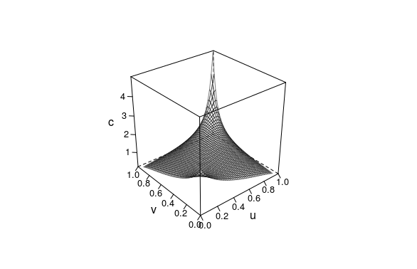
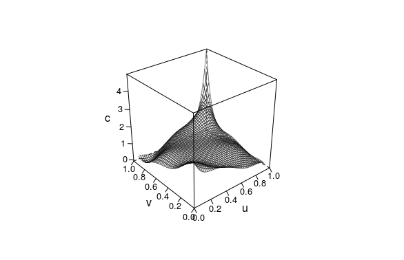
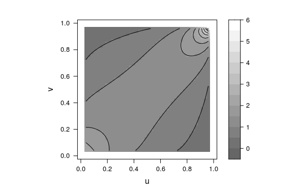
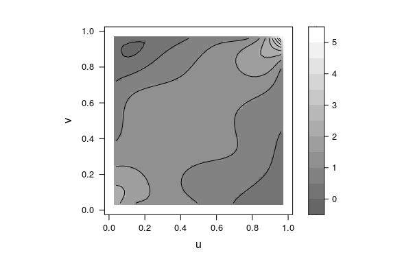
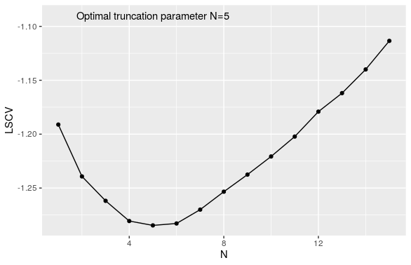
Figure 1: Loss-ALAE data.
Upper: Gumbel copula density with parameter $1.45$ (left); $\widehat{c}^{[\mathbf{N}]}$ with $\mathbf{N}=5$ (right).
Middle: Gumbell contours lines (left); $\widehat{c}^{[\mathbf{5}]}$ contours lines (right).
Bottom: panel the rank-rank plot (left); the LSCV function (right).

log returns		Min	Max	Mean	Median	std.Dev.	Skewness	Kurtosis	JB P-value
	EUR	-4.204e-02	4.735e-02	-2.000e-07	-7.351e-05	0.006754196	0.08255672	3.438804	0
	GBP	-4.115e-02	8.321e-02	5.298e-05	6.305e-05	0.006614447	0.76795970	9.838880	0
	YEN	-4.309e-02	5.017e-02	2.174e-05	0.000e+00	0.006867485	0.19770234	3.835367	0
	CAD	-6.150e-02	6.150e-02	2.965e-05	-7.506e-05	0.006385885	0.05111347	13.485304	0
	AUD	-7.808e-02	1.015e-01	-3.152e-05	-1.840e-04	0.008720500	0.58507427	11.130791	0
	CHF	-8.390e-02	1.547e-01	8.765e-05	0.000e+00	0.007625693	1.64779228	43.205732	0

Table 8: Descriptive statistics for daily log returns

cop	$n$	$\tau$	MK-SE	MISE	$N$
Clayton	$500$	$0.3$	16.47(10.57)	3.98( 4.51)	4
		$0.55$	59.39(5.53)	34.44(6.56)	10
		$0.8$	61.10(2.90)	36.54(3.54)	18
	$1000$	$0.3$	10.12(5.99)	1.60(1.69)	3
		$0.55$	60.47(3.73)	35.40( 4.40)	11
		$0.8$	57.25(2.46)	31.98(2.79)	20
Gumbel	$500$	$0.3$	67.59( 4.22)	39.77(4.91)	6
		$0.55$	52.70(4.52)	25.52(4.36)	3
		$0.8$	71.33(0.92)	46.31(1.24)	10
	$1000$	$0.3$	54.36( 5.29)	25.91(4.95)	4
		$0.55$	33.02(5.58)	10.64( 3.53)	11
		$0.8$	68.81(0.80)	42.78(1.04)	14

Table 9: Bivariate copula densities using shrinkage function: Relative MK-SE and relative MISE in percentages and in brackets the minimun of standard deviation for the corresponding copula.

	EUR	GBP	YEN	CAD	AUD
GBP	10
YEN	3	5
CAD	8	7	7
AUD	7	10	5	11
CHF	16	9	7	5	5

Table 10: Optimal parameter $N$ for daily log-returns

	EUR	GBP	YEN	CAD	AUD
GBP	0.4367622
YEN	-0.148341452	-0.119612388
CAD	-0.182688503	-0.163666875	0.006203468
AUD	0.2668624	0.2555104	-0.1018401	-0.1843126
CHF	-0.6308960	-0.3978123	0.2055829	0.1277914	-0.2176760

Table 11: Kendall’s rank correlations for daily log-returns

References

- Abramowitz and Stegun, (1970) Abramowitz, M. and Stegun, I. A. (1970). Handbook of mathematical functions with formulas, graphs, and mathematical tables, volume 55. US Government printing office.
- Autin et al., (2010) Autin, F., Le Pennec, E., and Tribouley, K. (2010). Thresholding methods to estimate copula density. Journal of Multivariate Analysis, 101(1):200–222.
- Beare, (2010) Beare, B. K. (2010). Copulas and temporal dependence. Econometrica, 78(1):395–410.
- Boas Jr, (1969) Boas Jr, R. (1969). Inequalities for the derivatives of polynomials. Mathematics Magazine, 42(4):165–174.
- Bouezmarni et al., (2013) Bouezmarni, T., El Gouch, A., and Taamouti, A. (2013). Bernstein estimator for unbounded copula densities. Statistics & risk modeling., 30(4):343–360.
- Bouezmarni et al., (2010) Bouezmarni, T., Rombouts, J. V., and Taamouti, A. (2010). Asymptotic properties of the bernstein density copula estimator for -mixing data. Journal of Multivariate Analysis, 101(1):1–10.
- Bowman, (1984) Bowman, A. W. (1984). An alternative method of cross-validation for the smoothing of density estimates. Biometrika, 71(2):353–360.
- Carley and Taylor, (2002) Carley, H. and Taylor, M. (2002). A new proof of sklar’s theorem. In Distributions with given marginals and statistical modelling, pages 29–34. Springer.
- Charpentier et al., (2007) Charpentier, A., Fermanian, J.-D., and Scaillet, O. (2007). The estimation of copulas: Theory and practice. Copulas: From theory to application in finance, pages 35–64.
- Chatelain et al., (2020) Chatelain, S., Fougères, A.-L., Neslehová, J. G., et al. (2020). Inference for archimax copulas. Annals of Statistics, 48(2):1025–1051.
- Chatrabgoun et al., (2017) Chatrabgoun, O., Parham, G., and Chinipardaz, R. (2017). A legendre multiwavelets approach to copula density estimation. Statistical Papers, 58(3):673–690.
- Chen and Fan, (2005) Chen, X. and Fan, Y. (2005). Pseudo-likelihood ratio tests for semiparametric multivariate copula model selection. Canadian Journal of Statistics, 33(3):389–414.
- Chen et al., (2010) Chen, X., Fan, Y., Pouzo, D., and Ying, Z. (2010). Estimation and model selection of semiparametric multivariate survival functions under general censorship. Journal of Econometrics, 157(1):129–142.
- Cohen et al., (2001) Cohen, A., DeVore, R., Kerkyacharian, G., and Picard, D. (2001). Maximal spaces with given rate of convergence for thresholding algorithms. Applied and Computational Harmonic Analysis, 11(2):167–191.
- Deheuvels, (1979) Deheuvels, P. (1979). La fonction de dépendance empirique et ses propriétés. un test non paramétrique d’indépendance. Bulletins de l’Académie Royale de Belgique, 65(1):274–292.
- Denuit et al., (2006) Denuit, M., Purcaru, O., and Keilegom, I. V. (2006). Bivariate archimedean copula models for censored data in non-life insurance. Journal of Actuarial Practice 1993-2006. 5.
- Efromovich, (2008) Efromovich, S. (2008). Nonparametric curve estimation: methods, theory, and applications. Springer Science & Business Media.
- Frees and Valdez, (1998) Frees, E. W. and Valdez, E. A. (1998). Understanding relationships using copulas. North American actuarial journal, 2(1):1–25.
- Geenens et al., (2017) Geenens, G., Charpentier, A., Paindaveine, D., et al. (2017). Probit transformation for nonparametric kernel estimation of the copula density. Bernoulli, 23(3):1848–1873.
- Genest et al., (2009) Genest, C., Masiello, E., and Tribouley, K. (2009). Estimating copula densities through wavelets. Insurance: Mathematics and Economics, 44(2):170–181.
- Genest et al., (2006) Genest, C., Quessy, J.-F., and Rémillard, B. (2006). Goodness-of-fit procedures for copula models based on the probability integral transformation. Scandinavian Journal of Statistics, 33(2):337–366.
- Gijbels and Mielniczuk, (1990) Gijbels, I. and Mielniczuk, J. (1990). Estimating the density of a copula function. Communications in Statistics-Theory and Methods, 19(2):445–464.
- Goldenshluger and Lepski, (2014) Goldenshluger, A. and Lepski, O. (2014). On adaptive minimax density estimation on . Probability Theory and Related Fields, 159(3-4):479–543.
- Hamdan and Al-Bayyati, (1971) Hamdan, M. and Al-Bayyati, H. (1971). Canonical expansion of the compound correlated bivariate poisson distribution. Journal of the American Statistical Association, 66(334):390–393.
- Janssen et al., (2014) Janssen, P., Swanepoel, J., and Veraverbeke, N. (2014). A note on the asymptotic behavior of the bernstein estimator of the copula density. Journal of Multivariate Analysis, 124:480–487.
- Joe, (2014) Joe, H. (2014). Dependence modeling with copulas. CRC press.
- Kauermann et al., (2013) Kauermann, G., Schellhase, C., and Ruppert, D. (2013). Flexible copula density estimation with penalized hierarchical b-splines. Scandinavian Journal of Statistics, 40(4):685–705.
- Klugman and Parsa, (1999) Klugman, S. A. and Parsa, R. (1999). Fitting bivariate loss distributions with copulas. Insurance: mathematics and economics, 24(1-2):139–148.
- Ko and Hjort, (2019) Ko, V. and Hjort, N. L. (2019). Model robust inference with two-stage maximum likelihood estimation for copulas. Journal of Multivariate Analysis, 171:362–381.
- Lancaster, (1958) Lancaster, H. O. (1958). The Structure of Bivariate Distributions. The Annals of Mathematical Statistics, 29(3):719 – 736.
- Massart, (1990) Massart, P. (1990). The tight constant in the dvoretzky-kiefer-wolfowitz inequality. The annals of Probability, pages 1269–1283.
- McNeil et al., (2015) McNeil, A. J., Frey, R., and Embrechts, P. (2015). Quantitative risk management: concepts, techniques and tools-revised edition. Princeton university press.
- Nagler, (2018) Nagler, T. (2018). kdecopula: An R package for the kernel estimation of bivariate copula densities. Journal of Statistical Software, 84(7):1–22.
- Nelsen, (2007) Nelsen, R. B. (2007). An introduction to copulas. Springer Science & Business Media.
- Omelka et al., (2009) Omelka, M., Gijbels, I., and Veraverbeke, N. (2009). Improved kernel estimation of copulas: weak convergence and goodness-of-fit testing. The Annals of Statistics, 37(5B):3023–3058.
- Pérez and Prieto-Alaiz, (2016) Pérez, A. and Prieto-Alaiz, M. (2016). A note on nonparametric estimation of copula-based multivariate extensions of spearman’s rho. Statistics & Probability Letters, 112:41–50.
- Qu and Yin, (2012) Qu, L. and Yin, W. (2012). Copula density estimation by total variation penalized likelihood with linear equality constraints. Computational Statistics & Data Analysis, 56(2):384–398.
- Rudemo, (1982) Rudemo, M. (1982). Empirical choice of histograms and kernel density estimators. Scandinavian Journal of Statistics, pages 65–78.
- Sancetta and Satchell, (2004) Sancetta, A. and Satchell, S. (2004). The bernstein copula and its applications to modeling and approximations of multivariate distributions. Econometric theory, pages 535–562.
- Segers et al., (2017) Segers, J., Sibuya, M., and Tsukahara, H. (2017). The empirical beta copula. Journal of Multivariate Analysis, 155:35–51.
- Sklar, (1959) Sklar, A. (1959). Fonction de répartition dont les marges sont données. Inst. Stat. Univ. Paris, 8:229–231.
- Taylor, (1990) Taylor, C. C. (1990). Orthogonal series estimators and cross-validation. Journal of Statistical Computation and Simulation, 37(3-4):151–158.
- Tsybakov, (2003) Tsybakov, A. B. (2003). Introduction à l’estimation non paramétrique, volume 41. Springer Science & Business Media.