Coherence dynamics induced by attenuation and amplification Gaussian channels

Abstract

Quantum Gaussian channels play a key role in quantum information theory. In particular, the attenuation and amplification channels are useful to describe noise and decoherence effects on continuous variables systems. They are directly associated to the beam splitter and two-mode squeezing operations, which have operational relevance in quantum protocols with bosonic models. An important property of these channels is that they are Gaussian completely positive maps and the action on a general input state depends on the parameters characterizing the channels. In this work, we study the coherence dynamics introduced by these channels on input Gaussian states. We derive explicit expressions for the coherence depending on the parameters describing the channels. By assuming a displaced thermal state with initial coherence as input state, for the attenuation case it is observed a revival of the coherence as a function of the transmissivity coefficient, whereas for the amplification channel the coherence reaches asymptotic values depending on the gain coefficient. Further, we obtain the entropy production for these class of operations, showing that it can be reduced by controlling the parameters involved. We write a simple expression for computing the entropy production due to the coherence for both channels. This can be useful to simulate many processes in quantum thermodynamics, as finite-time driving on bosonic modes.

I Introduction

In the last years, considerable effort has been dedicated to the comprehension and application of bosonic continuous variables. The interest ranges from quantum information theory Wang2007 ; Weedbrook2012 ; Adesso2014 , with direct implications in quantum communication and quantum computation Marshall2019 , to quantum thermodynamics Macchiavello2020 , where bosonic systems may work as working substance in quantum heat machines models Kosloff2017 and employed as ancillary systems in structured thermal reservoir designs Chiara2018 . As in general a system of interest is constantly interacting with its surrounding, bosonic Gaussian channels are particularly powerful to describe noise and decoherence in optical systems. There are two well-known bosonic Gaussian channels, the attenuation and amplification channels Weedbrook2012 ; SerafiniBook , as well as their limit cases, namely the quantum-limited attenuator and the quantum-limited amplification. The concatenation of the last two channels may be employed to represent any phase-insensitive channel in quantum optic processes SerafiniBook .

The actions of attenuation or amplification channels over a Gaussian input state may be physically understood by the effect on the first moments, resulting in a different output state. For the former, the first moments of the output state are reduced depending on the value of the transmissivity coefficient, whereas for the latter the output state has its first moments enlarged given a value of gain coefficient. Besides the emulation of noise and decoherence, the attenuation and amplification channels are associated to the beam splitter and two-mode squeezing operations Weedbrook2012 ; SerafiniBook , respectively, and thus directly related to the optical parametric down-conversion. Moreover, the study of the capacity of Gaussian channels is an essential task for any quantum communication protocol with continuous variables Jarzyna2017 ; Qi2017 . For example, it has been shown that attenuation and amplification channels transmit entanglement more efficiently when the input state are non-Gaussian than Gaussian Filippov2014 , as well as they have been employed in continuous variable quantum-key distribution Ruppert2019 ; Blandino2012 and quantum cloning optimization Braunstein2001 . The connection of these type of channels to non-Markovianity has been pointed in Ref. Liuzzo-Scorpo2017 .

The attenuation and amplification channels are well-known as Gaussian completely positive (GCP) maps and they perform Gaussian operations on input Gaussian states. On its turn, Gaussian operations are crucial in many areas, such as quantum information science and quantum thermodynamics. Depending on the process to be considered, Gaussian operations can produce coherence on a given input state Aroch . Recently, coherence effects have been addressed in different branches of quantum physics, for instance, in unitary process in quantum thermodynamics where, in particular, assuming a driven Hamiltonian that does not commute in different times will generate coherence in the system state Camati2019 , as well as the investigation of coherence as a resource in charging a quantum battery Garc=0000EDa-Pintos2020 . In particular, the concept of quantum friction, directly associated to the notion of finite-time regime in quantum protocols, has been described in terms of coherence in a specific basis Rezek2010 ; Plastina2014 . Moreover, some studies have associated an extra entropy production cost to the presence of coherence in the state before the thermalization Jader2019 ; Francica2019 . Besides coherence in quantum states, the study of coherence in quantum channels has been investigated in Datta2018 ; Xu2019 . Thus, controlling the coherence dynamics of a specific protocol is certainly relevant, because the mitigation of coherence could to optimize the energy cost of a process.

In this work, we are interested in studying the coherence dynamics generated by the attenuation and amplification Gaussian channels over input Gaussian states. Given the high precision control in quantum optical platforms and its ability to generate these kind of Gaussian channels, a detailed investigation of how they influence the initial coherence of an input Gaussian state could be useful to design experiments with bosonic Gaussian channels, as wells as their application in quantum thermodynamics. Thus, we consider an input Gaussian state with initial coherence whose dynamics is dictated by the attenuation (amplification) channel. Employing a recent quantifier of coherence for Gaussian states, we provide explicit expressions for the coherence dynamics for these channels as functions of the parameters characterizing their actions. Besides, motivated by recent investigations concerning the entropy production in non-equilibrium quantum thermodynamics, we also study the role performed by the attenuation (amplification) channel in the entropy production. This could be useful for current and future experimental realization in quantum thermodynamics and quantum information.

The manuscript is organized as follows. In section II we review the main aspects and tools concerning the description of $N$- mode Gaussian states and how to represent the attenuation and amplification channel and parameterize them in terms of the beam splitter and two-mode squeezing operations, respectively. We present our first result in section III, where we derive the coherence for a single-mode input Gaussian state passing through the Gaussian channels referred above. Then, we generalize the results by assuming a $N$- mode input Gaussian state in which each mode is affected by an attenuation or amplification channel. Based on recent advances in quantum thermodynamics, in section IV we study how the coherence dynamics introduced by the Gaussian channels considered affects the entropy production during a thermalization process. We derive analytical expression for that in terms of the parameters characterizing the channels. Finally, in section V we draw our conclusion and final remarks.

II Gaussian states and Gaussian channels

In this section we introduce the basic tools concerning the notion of Gaussian states and the class of phase-insensitive Gaussian channels, and how to characterize them, depending on the action on input Gaussian states.

Gaussian states have been largely applied in many branches of physics. They are experimental accessed in platforms such as quantum optics WallsBook and trapped ions Ortiz-Guti=0000E9rrez2017 . Their modern applications ranging from quantum information theory Wang2007 ; Weedbrook2012 ; Adesso2014 to quantum thermodynamics Macchiavello2020 ; Kosloff2017 . In order to characterize the class of Gaussian states, we define the quadrature operators vector $\vec{R}=\left(q_{1},p_{1},...q_{N},p_{N}\right)$, where $N$ is the number of modes of a given system, and $\left(q,p\right)$ stand for position and momentum, respectively. Gaussian states are completely determined by the first moments and the covariance matrix, which are defined as $\vec{d}=\langle\vec{R}\rangle_{\rho}$ and $\sigma_{ij}=\langle R_{i}R_{j}+R_{j}R_{i}\rangle_{\rho}-2\langle R_{i}\rangle_{\rho}\langle R_{j}\rangle_{\rho}$, respectively, with $\rho=\rho(\vec{d},\sigma)$ the state of the system. For a $N$-mode Gaussian state $\rho=\rho_{1}\otimes\rho_{2}\otimes...\otimes\rho_{N}$, the associated first moments and covariance matrix are given by the simple relations

$$\vec{d} =\vec{d}_{1}\oplus\vec{d}_{2}\oplus...\oplus\vec{d}_{N},$$ (1)

$$\sigma =\sigma_{1}\oplus\sigma_{2}\oplus...\oplus\sigma_{N}.$$ (2)

The well-known example of single-mode Gaussian states is the thermal state, with null first moments and covariance matrix given by $\sigma^{th}=(2\bar{n}+1)\mathbb{I}_{2}$, with $\bar{n}=\text{Tr}\left[a^{\dagger}a\right]$ the average number of photons in a mode, $a$ ($a^{\dagger}$) the annihilation (creator) operator, and $\mathbb{I}_{2}$ an identity matrix of order 2. Thermal states are written in the Fock basis as

$$\rho^{th}(\bar{n})=\sum_{n}\frac{\bar{n}^{n}}{\left(\bar{n}+1\right)^{n+1}}|n\rangle\langle n|$$ (3)

Other examples, as the displaced thermal state, is obtained by acting the Weyl operator on a general thermal state, while the coherent state can be defined by the same action but with $\bar{n}=0$ WallsBook .

Most part of the applications in quantum information theory and related fields consider a dynamics where the system of interest (input state) interacts with an ancillary one (ancilla) prepared in a Gaussian state, also known as the environment. When a given protocol is implemented through a quadratic Hamiltonian, then after tracing out the ancilla, the Gaussianity of the initial input state is preserved SerafiniBook . The set of operations with this property are known as Gaussian completely positive maps (GCP maps) or channels, being useful to describe noise and decoherence effects on input Gaussian states. The complete characterization of GCP maps on input Gaussian states can be represented by SerafiniBook

$$\vec{d} \rightarrow\mathcal{F}\vec{d},$$ (4)

$$\sigma \rightarrow\mathcal{F}\sigma\mathcal{F}^{T}+\mathcal{G},$$ (5)

with $\mathcal{F}$ and $\mathcal{G}$ two $2N\times 2N$ real matrices satisfying the relation $\mathcal{G}+i\Omega\geq i\mathcal{F}\Omega\mathcal{F}^{T}$where $\Omega=\left(\begin{array}[]{cc}0&1\\ -1&0\end{array}\right)$. Among different GCP maps which can be implemented, we are interested in the well-known attenuation and amplification channels, also called phase-insensitive Gaussian channels, which are responsible by many optical processes of interest in quantum information theory Wang2007 ; Weedbrook2012 ; Adesso2014 . The action of these channels on a single-mode input Gaussian state can be written in terms of the quadrature operators vector. Following Ref. Weedbrook2012 the attenuation channel is represented by

$$\vec{R}\rightarrow\sqrt{\tau}\vec{R}+\sqrt{1-\tau}\vec{R}_{th},$$ (6)

where $0<\tau<1$ is known as the transmissivity coefficient and $\vec{R}_{th}$ is the quadrature operator of the thermal state of the environment with average number of photons $\bar{m}$. Similarly, the amplification channel is given by

$$\vec{R}\rightarrow\sqrt{g}\vec{R}+\sqrt{g-1}\vec{R}_{th},$$ (7)

with $g>1$ the gain coefficient. We can parameterize these channels by writing $\tau=\cos^{2}\theta$ and $g=\cosh^{2}r$ such that the attenuation channel is identified to the action of a beam splitter, whereas the amplification channel is identified to the action of a two-mode squeezing transformation SerafiniBook . In doing so, we are able to represent the attenuation ($\mathcal{E}_{\theta}^{\bar{m}}$) and the amplification ($\mathcal{A}_{r}^{\bar{m}}$) channels using Eqs. (4) and (5) i.e.,

$$\mathcal{E}_{\theta}^{\bar{m}} :$$ (8)

$$\mathcal{F}_{\text{att}} =\cos\theta\mathbb{I}_{2}$$ (9)

$$\mathcal{G}_{\text{att}} =(2\bar{m}+1)\sin^{2}\theta\mathbb{I}_{2},$$ (10)

with $\theta\in[0,2\pi[$, and

$$\mathcal{A}_{r}^{\bar{m}} :$$ (11)

$$\mathcal{F}_{\text{amp}} =\cosh r\mathbb{I}_{2}$$ (12)

$$\mathcal{G}_{\text{amp}} =(2\bar{m}+1)\sinh^{2}r\mathbb{I}_{2},$$ (13)

with $r\in[0,\infty[$.

There are two limit cases which will be useful in the following, and they are found by assuming $\bar{m}=0$. For the attenuation channel, this results in an operation known as quantum limited attenuator. In this limit, when the input state is a coherent state, the covariance matrix remains unchanged. For the amplification channel, imposing $\bar{m}=0$ implies in the channel known as quantum limited amplifier, meaning that, a minimum noise is added in the covariance matrix of the input state. It is possible to show that any single-mode phase-insensitive Gaussian channel can be written using the quantum limited attenuator and the quantum limited amplifier channels SerafiniBook , i.e,

$$\mathcal{E^{\text{ph}}} =\mathcal{A}_{r}^{0}\circ\mathcal{E}_{\theta}^{0}:$$ (14)

$$\mathcal{F}_{\text{ph}} =\cosh r\cos\theta\mathbb{I}_{2}$$ (15)

$$\mathcal{G}_{\text{ph}} =\left(\cosh^{2}r\sin^{2}\theta+\sinh^{2}r\right)\mathbb{I}_{2}.$$ (16)

This channel is particularly important to study the information capacity of bosonic channels SerafiniBook .

III Coherence in attenuation and amplification channels

The investigation of coherence in quantum systems is an active field in quantum information theory Plenio2014 ; Winter2016 ; Dana2017 , quantum thermodynamics Macchiavello2020 and related areas Ralph2003 ; Joo2011 . Given an initial state $\rho_{0}$ subject to a given protocol represented by a map $\Lambda_{\tau,0}$, the ability to quantify the coherence of the final state $\rho_{\tau}=\Lambda_{\tau,0}\left[\rho_{0}\right]$ is an important task. Since the coherence depends on the particular choice of a basis, we use here the Fock basis $\left\{|N\rangle\right\}_{0}^{\infty}$, which has the advantage to be associated to the eigenvalues of energy of a system. Following Ref. Plenio2014 , to introduce an entropic quantifier of coherence we must define a set of incoherent states. From Ref. Xu2016 , for general Gaussian states the set of incoherent states are given by the thermal states, which are Gibbs states and do not present coherence in the Fock basis. By defining a reference state as being a thermal one $\zeta=\rho^{th}(\bar{k})$ we can write an entropic quantifier of coherence of a Gaussian state $\rho$ as $C(\rho)=\text{min}_{\zeta}\left[S\left(\rho||\zeta\right)\right]$ with $S\left(\rho_{1}||\rho_{2}\right)=\text{Tr$\left[\rho_{1}\text{ln}\rho_{1}\right]$}-\text{Tr}\left[\rho_{1}\text{ln}\rho_{2}\right]$ the relative entropy and the minimization is performed on all the thermal states $\zeta$.

Following Ref. Xu2016 , an entropic measure for coherence of a $N$-mode Gaussian state $\rho=\rho(\vec{d},\sigma)$ is given by

$$C(\rho)=S(\zeta)-S(\rho),$$ (17)

where $S(\cdot)$ is the von Neumann entropy,

$$S(\rho)=-\sum_{j=1}^{N}\left[\frac{\nu_{j}-1}{2}\ln\left(\frac{\nu_{j}-1}{2}\right)-\frac{\nu_{j}+1}{2}\ln\left(\frac{\nu_{j}+1}{2}\right)\right],$$ (18)

with $\left\{\nu_{j}\right\}_{j=1}^{N}$ the symplectic eigenvalues of $\sigma$, and $\zeta$ is a $N$-mode reference thermal state with average number of photons $\left\{\bar{k}_{j}\right\}_{j=1}^{N}$written in terms of the first moments and the covariance matrix of the input state and given by

$$\bar{k}_{j}=\frac{1}{4}\left[\sigma_{11}^{j}+\sigma_{22}^{j}+\left(d_{1}^{j}\right)^{2}+\left(d_{2}^{j}\right)^{2}-2\right].$$ (19)

The coherence quantifier in Eq. (17) satisfies the following properties: $C(\rho)\geq 0$, $C(\rho)=0$ if and only if $\rho$ is a tensor product of thermal states, $C(\rho)\geq C(\Phi_{IGC}\rho)$, where $\Phi_{IGC}$ is an incoherent Gaussian channel Xu2016 . In the following, we consider the problem of a single-mode input Gaussian state. Then, we generalize our results for a $N$-mode input Gaussian state.

One-mode input state

Consider a single-mode input Gaussian state $\rho=\rho(\vec{d},\sigma)$ passing through a Gaussian channel as depicted in Fig. 1-a). The channel can be an attenuation or an amplification one, and the ancilla is assumed to be a Gaussian state with average number of photons $\bar{m}$ in both cases. We consider that the single-mode input state is Gaussian, more specifically, it is a displaced thermal state with first moments $\vec{d}=\left(q_{0},p_{0}\right)$ and covariance matrix $\sigma=\left(2\bar{n}+1\right)\mathbb{I}_{2}$. Using Eq. (17) for the attenuation channel introduced in Eq. (8), the coherence quantifier can be written in a compact form as

$$C_{\text{att}}(\rho) =\frac{A_{\text{att}}-1}{2}\ln\left[\frac{A_{\text{att}}-1}{2}\right]$$

$$-\frac{A_{\text{att}}+1}{2}\ln\left[\frac{A_{\text{att}}+1}{2}\right]$$

$$+B_{\text{att}}\ln\left[B_{\text{att}}\right]-\left(B_{\text{att}}-1\right)\ln\left[B_{\text{att}}-1\right],$$ (20)

where

$$A_{\text{att}} =\left(2\bar{n}+1\right)\cos^{2}\theta+(2\bar{m}+1)\sin^{2}\theta,$$ (21)

$$B_{\text{att}} =\frac{1}{2}\left(\left(2\bar{n}+1\right)\cos^{2}\theta+\left(2\bar{m}+1\right)\sin^{2}\theta\right)$$ (22)

$$+\frac{1}{4}\left[\left(q_{0}^{2}+p_{0}^{2}\right)\cos^{2}\theta-2\right]+1.$$ (23)

For the amplification channel, a similar calculation provides the following expression for the coherence

$$C_{\text{amp}}(\rho) =\frac{A_{\text{amp}}-1}{2}\ln\left[\frac{A_{\text{amp}}-1}{2}\right]$$

$$-\frac{A_{\text{amp}}+1}{2}\ln\left[\frac{A_{\text{amp}}+1}{2}\right]$$

$$+B_{\text{amp}}\ln\left[B_{\text{amp}}\right]-\left(B_{\text{amp}}-1\right)\ln\left[B_{\text{amp}}-1\right]$$ (24)

where

$$A_{\text{amp}} =\left(2\bar{n}+1\right)\cosh^{2}r+(2\bar{m}+1)\sinh^{2}r,$$ (25)

$$B_{\text{amp}} =\frac{1}{2}\left(\left(2\bar{n}+1\right)\cosh^{2}r+\left(2\bar{m}+1\right)\sinh^{2}r\right)$$ (26)

$$+\frac{1}{4}\left[\left(q_{0}^{2}+p_{0}^{2}\right)\cosh^{2}r-2\right]+1.$$ (27)

In order to illustrate the coherence dynamics introduced by the attenuation and amplification channels on the single-mode input Gaussian state, we consider the initial first moments to be $\left(q_{0},p_{0}\right)=\left(1,1\right)$ in arbitrary unity, an average number of photons $\bar{n}=4$ for the input state. Figure 2 illustrates the coherence quantifier for the attenuation (figure a)) and the amplification (figure b)) channels, as a function of the parameter $\theta$ and $r$, respectively.

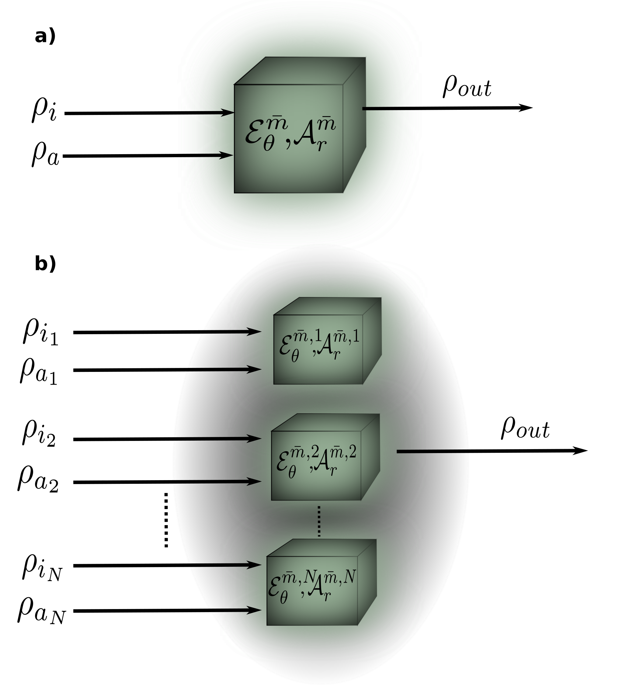
Figure 1: Action of Gaussian channels. a) A single-mode input Gaussian state passes through an attenuation (amplification) channel parameterized by the parameters $\bar{m}$ and $\theta$ ($\bar{m}$ and $r$). Since the input state is assumed to have an initial amount of coherence, the coherence dynamics of the output state will depend on the Gaussian channel considered. b) Generalization to a $N$-mode input Gaussian state where each mode interacts with an attenuation (amplification) channel separately.

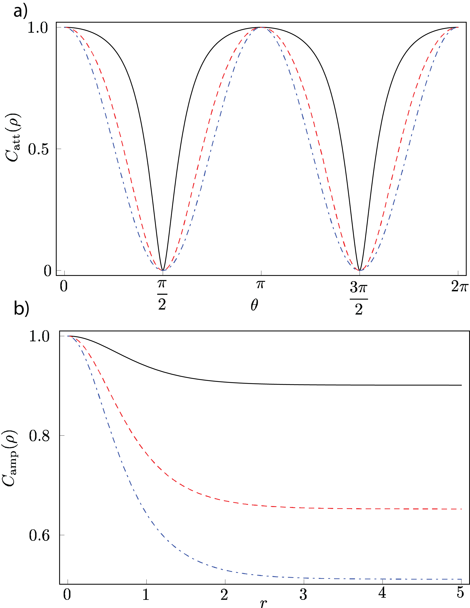
Figure 2: Normalized coherence quantifier of the output single-mode Gaussian state. a) Coherence of the output Gaussian state due to the attenuation channel. b) Coherence of the output Gaussian state due to the amplification channel. We consider an average number of photons $\bar{n}=4$ and initial first moments $(q_{0},p_{0})=(1,1)$ for the input state. For the thermal environment, we assume $\bar{m}=0$ (solid black line), $\bar{m}=2$ (red dashed line), and $\bar{m}=4$ (blue dotted dashed line). For $\bar{m}=0$ we have the quantum limited attenuator and the quantum limited amplifier, respectively.

Figure 2-a) shows that for the attenuation channel, the coherence of the single-mode input Gaussian state oscillates between its initial value and zero. Indeed, when $\theta=\pi/2$ and $3\pi/2$ the first moments of the output state are zero, and the input state, which was assumed to be a displaced thermal state, becomes a purely thermal one. It is possible also to note that the quantum limited attenuator, $\bar{m}=0$ (solid black line), represents the smoothest value of coherence at each maximum point. This could be interesting in protocols where the aim is to preserve the coherence in a wide range of a given parameter.

On the other hand, for the amplification Gaussian channel, Fig. 2-b) depicts the coherence of the single-mode output state as a function of the two-mode squeezing operation parameter $r$. We observe that, as expected, the quantum limited amplifier case, $\bar{m}=0$ (solid black line) means the minimum influence on the covariance matrix of the input state, implying in the maximum value of coherence in the asymptotic limit. At first sight, we could expect that the coherence introduced by the amplification channel would increase as the parameter $r$ becomes larger, by virtue of, for Gaussian states, the coherence increases as more distant the state is from the origin on the phase-space. However, we must take in account the action of the amplification channel on the covariance matrix of the input state, which is responsible for the behavior shown in Fig. 2-b). From Eq. (24) we are able to obtain the asymptotic value of coherence when $r\rightarrow 0$ and $r\rightarrow\infty$. They are given respectively by

$$C_{\text{amp}}^{r\rightarrow 0}(\rho) =\bar{n}\ln\left(\bar{n}\right)-\left(\bar{n}+1\right)\ln\left(\bar{n}+1\right)$$

$$+\left(\bar{n}+1+\frac{q_{0}^{2}+p_{0}^{2}}{4}\right)\ln\left(q_{0}^{2}+p_{0}^{2}+4\bar{n}+4\right)$$

$$-\left(\bar{n}+\frac{q_{0}^{2}+p_{0}^{2}}{4}\right)\ln\left(q_{0}^{2}+p_{0}^{2}+4\bar{n}\right)-2\ln(2),$$ (28)

and

$$C_{\text{amp}}^{r\rightarrow\infty}(\rho) =\ln\left(q_{0}^{2}+p_{0}^{2}+4\left(\bar{n}+\bar{m}+1\right)\right)$$

$$-\ln\left(\bar{n}+\bar{m}+1\right)-2\ln(2).$$ (29)

Equation (28) is nothing but the initial coherence of the single-mode input Gaussian state. On the other hand, Eq. (29) represents the maximum coherence that one achieves in the output state, despite the fact that its first moments increase as the parameter $r$ becomes larger. Another important limit we can investigate is when the average number of photons of the input state, $\bar{n}$, goes to infinity, i.e., the input state possesses considerable thermal fluctuation effects. In this case, Eqs. (20) and (24) result in $C_{\text{att}}^{\bar{n}\rightarrow\infty}=C_{\text{amp}}^{\bar{n}\rightarrow\infty}=0$, indicating that, if the input Gaussian state is highly thermal, then no coherence dynamics is introduced by the attenuation and the amplification channels. This is similar to the thermodynamic limit, in which $k_{B}T\gg\hbar\omega$.

To conclude our discussion about single-mode input states, we consider the concatenation of channels defined in Eq. (14). It is straightforward to note that the coherences displayed in Figs. 2-a) and 2-b) are marginals of the concatenation of the quantum limited attenuator and the quantum limited amplifier, i.e., the particular case of $\bar{m}=0$ (solid black lines).

N-mode input state

In order to generalize our results, we consider now a $N$-mode input Gaussian state formed by the tensor product of single-mode states, given by $\rho=\rho(\vec{d},\sigma)$, with $\vec{d}=\left(q_{1,0},p_{1,0},...,q_{N,0},p_{N,0}\right)$ and $\sigma=\sigma_{1,0}\oplus\sigma_{2,0}\oplus...\oplus\sigma_{N,0}$ the initial first moments and covariance matrix, respectively, and $\sigma_{j,0}=\left(2\bar{n}_{j}+1\right)\mathbb{I}_{2}$. The state $\rho$ passes through a GCP map composed of a series of independent attenuation (amplification) channels $\mathcal{E}_{\theta}^{\bar{m},j}$($\mathcal{A}_{r}^{\bar{m},j}$), as depicted in Fig. 2-b).

The coherence quantifier in this situation is a straightforward generalization of the one-mode case and, for the attenuation channel, it is given by

$$C_{\text{att}}(\rho) =-S(\rho)+\sum_{j=1}^{N}\left[\left(\bar{k}_{j}+1\right)\ln\left(\bar{k}_{j}+1\right)-\left(\bar{k}_{j}\right)\ln\left(\bar{k}_{j}\right)\right],$$ (30)

where

$$S(\rho)=-\sum_{j=1}^{N}\left[\frac{\nu_{j}-1}{2}\ln\left(\frac{\nu_{j}-1}{2}\right)-\frac{\nu_{j}+1}{2}\ln\left(\frac{\nu_{j}+1}{2}\right)\right],$$ (31)

with $\nu_{j}$ the symplectic eigenvalues of the output covariance matrix, given by

$$\nu_{j}=\left(2\bar{n}_{j}+1\right)\cos^{2}\theta+(2\bar{m}_{j}+1)\sin^{2}\theta,$$ (32)

and $\bar{k}_{j}$ is the $j$-th average number of photons associated to the $j$-th thermal reference state, and written as

$$\bar{k}_{j} =\frac{1}{2}\left(\left(2\bar{n}_{j}+1\right)\cos^{2}\theta+(2\bar{m}_{j}+1)\sin^{2}\theta\right)$$

$$+\frac{1}{4}\left(\cos^{2}\theta\left(q_{j,0}^{2}+p_{j,0}^{2}\right)-2\right),$$

whereas for the amplification channel one has

$$C_{\text{amp}}(\rho) =-S(\rho)+\sum_{j=1}^{N}\left[\left(\bar{k}_{j}+1\right)\ln\left(\bar{k}_{j}+1\right)-\left(\bar{k}_{j}\right)\ln\left(\bar{k}_{j}\right)\right],$$ (33)

where

$$S(\rho)=-\sum_{j=1}^{N}\left[\frac{\nu_{j}-1}{2}\ln\left(\frac{\nu_{j}-1}{2}\right)-\frac{\nu_{j}+1}{2}\ln\left(\frac{\nu_{j}+1}{2}\right)\right],$$ (34)

with $\nu_{j}$ the symplectic eigenvalues of the output covariance matrix, given by

$$\nu_{j}=\left(2\bar{n}_{j}+1\right)\cosh^{2}r+(2\bar{m}_{j}+1)\sinh^{2}r,$$ (35)

and $\bar{k}_{j}$ is the $j$-th average number of photons associated to the $j$-th thermal reference state, and written as

$$\bar{k}_{j} =\frac{1}{2}\left(\left(2\bar{n}_{j}+1\right)\cosh^{2}r+(2\bar{m}_{j}+1)\sinh^{2}r\right)$$

$$+\frac{1}{4}\left(\cosh^{2}r\left(q_{j,0}^{2}+p_{j,0}^{2}\right)-2\right).$$

Equations (30) and (33) are general in the sense that each attenuation (amplification) channel acting on each mode of the input state are free to have different average number of photons $\bar{m}_{j}$. Besides, although we have considered the same value of $\theta$ and $r$ for different $j$-th attenuation (amplification) channel, the expressions could be easily generalized for different values, corresponding to $\theta_{j}$ and $r_{j}$.

IV Connection to quantum thermodynamics

Quantum thermodynamics is a modern topic that will impact many technological areas such as quantum information science and quantum computation. On one hand, coherence plays important roles in quantum thermodynamics protocols. In particular, it is associated to the degradation or improvement of the performance of quantum thermal machines Chen2017 ; Camati2019 ; Zagoskin2012 , as well as it is used as a resource to several types of dynamics Winter2016 ; Dana2017 ; Kamin2020 . As we observed in Sec. III, depending on the value of parameters $\theta$ or $r$, the output states can have different amount of coherence for the attenuation or amplification channels, respectively. On the other hand, the entropy production is a relevant quantity in classical and quantum thermodynamics, mainly because it is associated to the irreversibility of a given protocol Jader2019 ; Gherardini2018 ; Deffner2011 . Besides, the increase of the entropy production due to the presence of coherence has been addressed in Ref. Jader2019 ; Francica2019 . Here we are interested in relating the coherence dynamics dictated by an attenuation (amplification) channel to the entropy production during a thermalization process. With this purpose in mind the following protocol (see Fig. 3) is assumed. The system, prepared in a displaced thermal state with average number of photons $\bar{n}$, interacts unitarily through an attenuation (amplification) channel. This process is adiabatic in the sense that there is no heat exchange. After that, the system thermalizes with a Markovian thermal reservoir with average number of photons $\bar{N}$ and inverse temperature $\beta=1/k_{B}T$, with $k_{B}$ the Boltzmann constant. The entropy production in this case can be written as (see Appendix Appendix. Entropy production)

$$\langle\Sigma\rangle=-\beta\Delta\mathcal{U}_{\tau_{2},\tau_{1}}+\Delta S_{\tau_{2},\tau_{1}},$$ (36)

where $\Delta\mathcal{U}_{\tau_{2},\tau_{1}}=\mathcal{U}_{\tau_{2}}-\mathcal{U}_{\tau_{1}}$ is the variation of internal energy associated to the thermalization process, with $\mathcal{U}_{t}=\text{Tr$\left[\sigma_{t}\right]$}/4$, and $\Delta S_{\tau_{2},\tau_{1}}=S(\rho_{\tau_{2}})-S(\rho_{\tau_{1}})$. The relation between the inverse temperature and the average number of photons of the reservoir is given by the Maxwell-Boltzmann distribution $\bar{N}=\left(e^{\beta\hbar\omega}-1\right)^{-1}$.

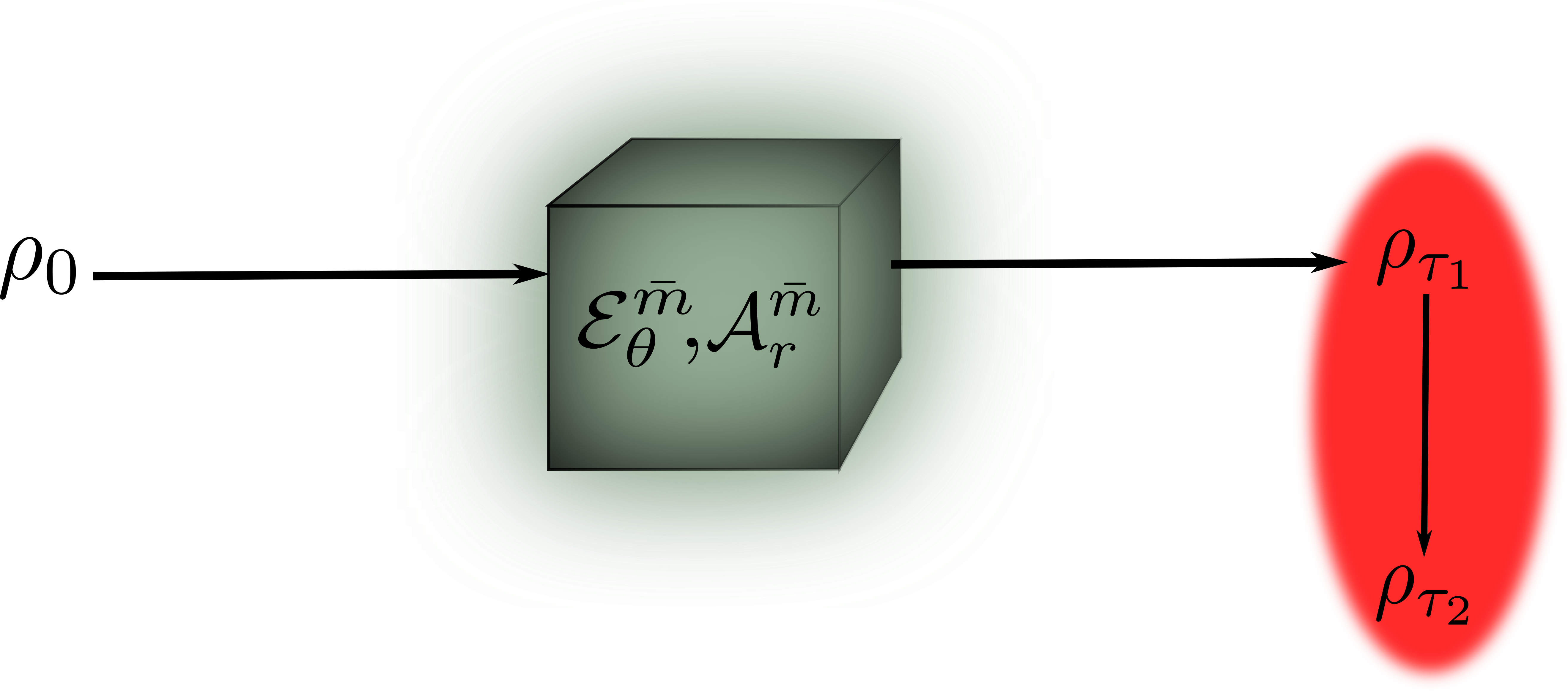
Figure 3: Entropy production. A single-mode input displaced thermal state $\rho_{0}$ passes through an attenuation (amplification) channel, which introduces a coherence dynamics on the output state $\rho_{\tau_{1}}$. After that, the system interacts with a Markovian heat reservoir and the final state $\rho_{\tau_{2}}$ is obtained. Depending on the allocation of the parameters $\theta$ ($r$), the coherence dynamics will result in a larger or lower amount of entropy production.

The dynamics of the state during the thermalization is given by the master equation PetruccioneBook ; SerafiniBook

$$\frac{d\rho}{dt}=\gamma\left(\bar{N}+1\right)\mathcal{D}\left[a\right]\rho+\gamma\bar{N}\mathcal{D}\left[a^{\dagger}\right]\rho,$$ (37)

with $\mathcal{D}[\mathcal{O}]=\mathcal{O}\rho\mathcal{O}^{\dagger}-(1/2)\left(\rho\mathcal{O}^{\dagger}\mathcal{O}+\mathcal{O}^{\dagger}\mathcal{O}\rho\right)$ the Lindblad operators and the decay rate $\gamma$. The same dynamics can be recasted by acting on the first moments and covariance matrix by employing the map $\mathcal{F}^{\text{therm}}=e^{-\gamma t/2}\mathbb{I}_{2}$ and $\mathcal{G}^{\text{therm}}=\left(2\bar{N}+1\right)\left(1-e^{-\gamma t}\right)\mathbb{I}_{2}$ in Eqs. (4) and (5) SerafiniBook .

To show how the coherence dynamics, introduced by the attenuation (amplification) channel, affects the thermalization process, in Fig. 4 (5) we present the entropy production as a function of the parameter $\theta$ ($r$) and of the thermalization time $t$ for the attenuation (amplification) channel, respectively. For both situations we consider $\bar{n}=1$, $\bar{m}=2,$ $\bar{N}=5$, and $\gamma=0.1\tau$. The parameter $\tau$ is introduced just to make the time dimensionless. Figure 4-a) shows the entropy production for the attenuation channel as a function of the thermalization time for $\theta=\pi/2$ (black solid lines) and $\theta=0$ (red dashed lines). From our results for the coherence in this class of channel, we note that the presence of coherence (dashed red line) has an additional entropy production cost. On the other hand, Fig. 4-b) depicts the entropy production as a function of the parameter $\theta$ fixing the thermalization time in $t/\tau=5$ (black solid line) (partial thermalization regime) and $t/\tau\approx T_{\text{th}}$(red dashed line) (complete thermalization regime), with $T_{\text{th}}$ being the time need to have complete thermalization. As expected, the values of $\theta$ for which there is no coherence ($\theta=\pi/2$ and $3\pi/2$) are those where the entropy production for complete or partial thermalization reaches a minimum.

Figure 5-a) illustrates the entropy production for the amplification channel as a function of the thermalization time for $r=0$ (dashed red line) and $r=0.5$ (solid black line). We observe that for $r=0.5$ the entropy production is smaller than for $r=0$ for all time interval. This happens because the coherence, as we see in Fig. 2-b), starts to decrease as $r$ becomes larger up to reach an asymptotic value. In Fig.5-b) we present the entropy production for the amplification channel as a function of the parameter $r$ for $t/\tau=5$ (black solid line), partial thermalization regime, and $t/\tau=T_{\text{th}}$ (red dashed line), complete thermalization regime. It can be noted that, the entropy production in both cases decreases up to a fixed value of $r$, when then it starts to increase, and it goes to infinity as $r\rightarrow\infty$. This change in the behavior of the entropy production is directly associated to the coherence dynamics in 2-b). We could argue that, for a given protocol where is expected to have a minimum entropy production, the simulation through an amplification channel could be useful, since the high control of the parameter $r$ is achievable.

From Figs. 4-a) and .5-a) it is also possible to conclude that the difference between the dashed red line and the solid black line represents exactly the entropy production contribution due to the coherence of the state $\rho_{\tau_{1}}$. In general, we can express this mathematically as

$$\langle\Sigma\rangle_{\text{coherence}}^{\alpha}=\langle\Sigma\rangle(\ell_{1})-\langle\Sigma\rangle(\ell_{0}),$$ (38)

where $\alpha$ stands for the attenuation (amplification) channel and $\ell$ for the parameter $\theta$ ($r$), such that $\ell_{0}=\pi/2$ ($r\rightarrow\infty)$ and $\ell_{1}=\theta$ ($r$), with $0\leq\theta\leq\pi/2$ and $0\leq r\leq\infty$. The hatched area in Figs. 4-a) and .5-a) means the quantity $\langle\Sigma\rangle_{\text{coherence}}^{\alpha}$ for different values of $\ell_{1}$. It must to be stressed that, for the amplification channel, $r\rightarrow\infty$ represents the minimum value of coherence that the output state $\rho_{\tau_{1}}$ can have, differently of the attenuation channel, in which the minimum value of coherence for the output state is zero.

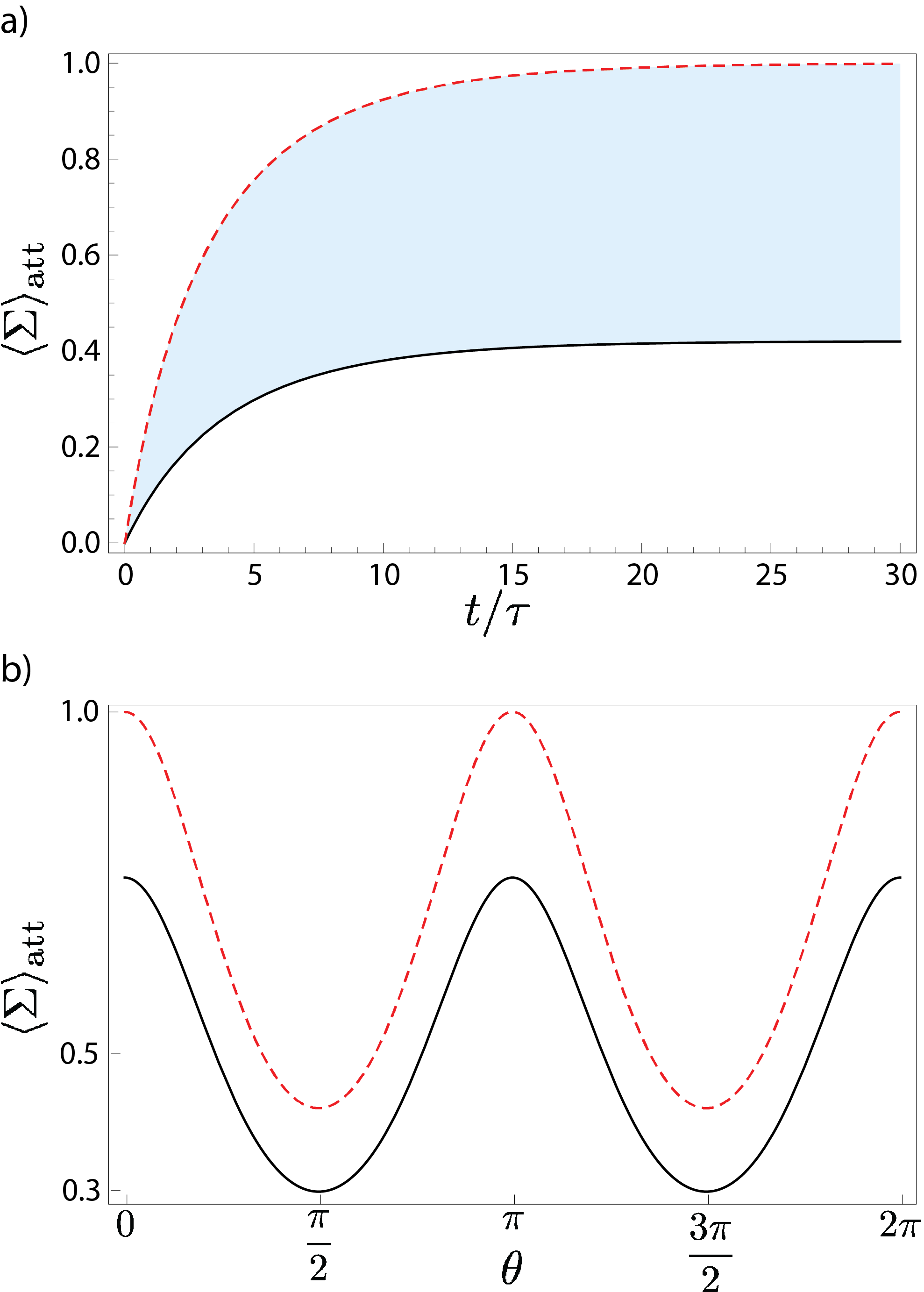
Figure 4: Entropy production for the attenuation channel. We assume the following protocol: the input state $\rho_{\text{in}}$ with average number of photons $\bar{n}$ passes through an attenuation channel characterized by an angle $\theta$ and average number of photons $\bar{m}$; then the output state $\rho_{\tau_{1}}$ thermalizes with a thermal reservoir with average number of photons $\bar{N}$ such that $\bar{N}>\bar{n}$. The final state of the thermalization is $\rho_{\tau_{2}}$. a) Entropy production as a function of the time of interaction with the thermal reservoir for $\theta=\pi/2$ (black solid line) and $\theta=0$ (red dashed line). The parameter $\tau$ is introduced just to make the time dimensionless. b) Entropy production as a function of the parameter $\theta$ for $t/\tau=5$ (black solid line) and $t/\tau=T_{\text{th}}$ (red dashed line). We considered $\bar{n}=1$, $\bar{m}=2$, $\bar{N}=5$, and $\gamma=0.1\tau$.

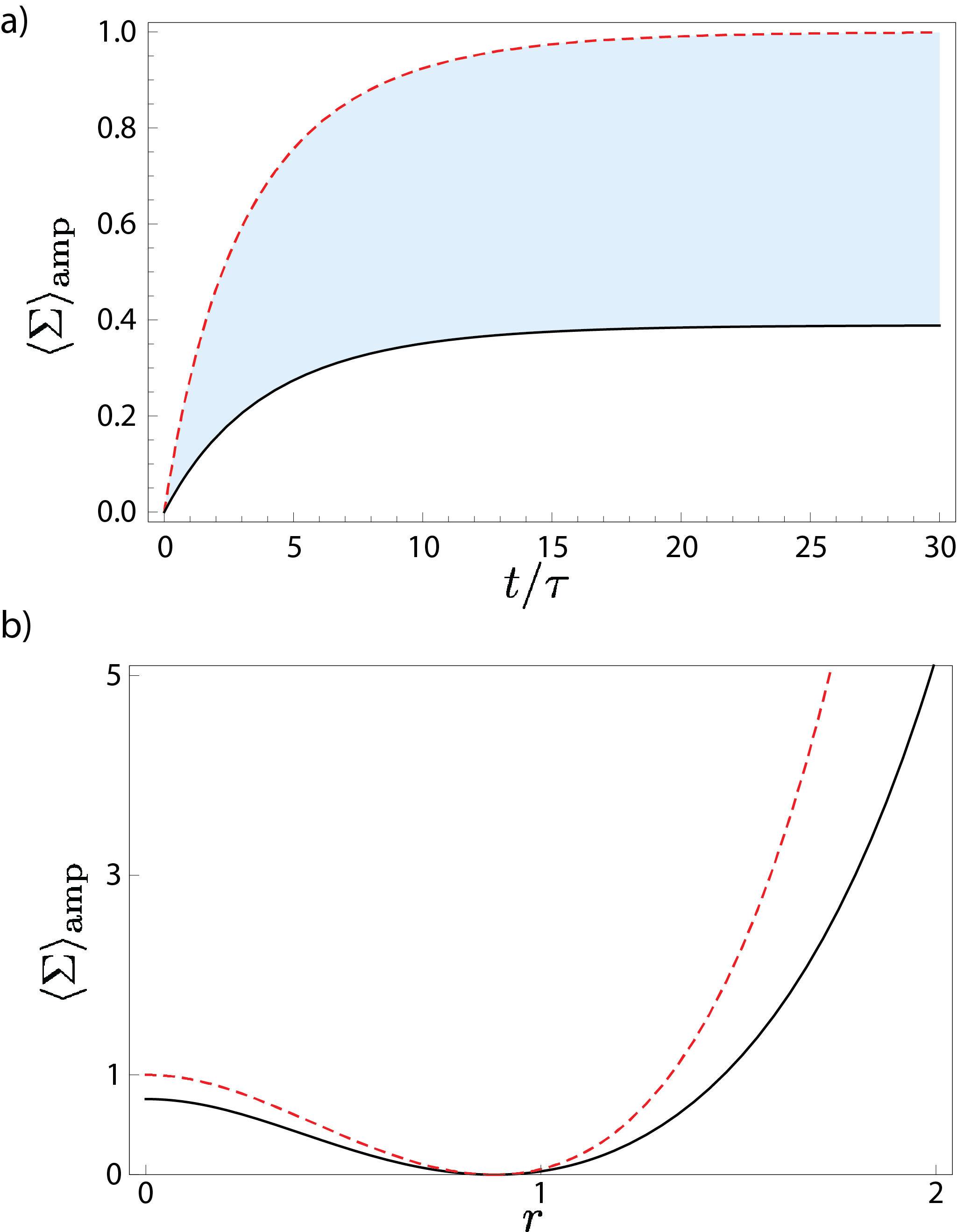
Figure 5: Entropy production for the amplification channel. We assume the following protocol: the input state $\rho_{\text{in}}$ with average number of photons $\bar{n}$ passes through an amplification channel characterized by an squeezing parameter $r$ and average number of photons $\bar{m}$; then the output state $\rho_{\tau_{1}}$ thermalizes with a thermal reservoir with average number of photons $\bar{N}$ such that $\bar{N}>\bar{n}$. The final state of the thermalization is $\rho_{\tau_{2}}$. a) Entropy production as a function of the time of interaction with the thermal reservoir for $r=0$ (red dashed line) and $r=0.5$ (black solid line). The parameter $\tau$ is introduced just to become the time dimensionless. b) Entropy production as a function of the parameter $r$ for $t=5/\tau$ (black solid line) and $t=T_{\text{th}}/\tau$ (red dashed line). We consider $\bar{n}=1$, $\bar{m}=2$, $\bar{N}=5$, and $\gamma=0.1\tau$.

V Conclusion

Gaussian channels play important role in continuous variables quantum information and thermodynamics protocols. In particular, attenuation and amplification channels are useful to describe the action of an environment on a input state, as noise and decoherence. As Gaussian operations, these channels can induce a coherence dynamics on a input Gaussian state depending on the choice of the channels parameters. In this work, we studied the how the attenuation and amplification channels affect the initial coherence of a input Gaussian state. We present analytical expressions for the coherence, showing that they can vary considerably as a function of the channel structure.

The entropy production of an attenuation (amplification) operation followed by an interaction with a Markovian thermal reservoir also was considered. We have shown that, depending on the precise allocation of the parameter in each type of channel, the entropy production can be reduced, such that the implementation of some protocol in quantum thermodynamics by means of the attenuation or amplification channels may be useful in experimental realizations. In particular, for the attenuation channel, it can be employed to simulate the transition between quasi-static and finite-time regimes in driven systems. Finally, for this class of channels we also write an expression relating the entropy production cost due to the coherence dynamics of a output state which thermalizes with a Markovian thermal reservoir. We hope that this work can contribute with current and future experimental propose to simulate thermodynamic process, as work extraction and quantum thermal cycles employing continuous variable systems.

Appendix. Entropy production

Although simple, here we derive the expression in Eq.(36). As mentioned in main text, the protocol is composed of two parts. The Gaussian input state passes through an attenuation (amplification) channel and then thermalizes with a Markovian thermal reservoir with inverse temperature $\beta$ and average number of photons $\bar{N}$. The entropy production of a unitary process followed by a thermalization can be written as Camati2019

$$\langle\Sigma\rangle=S(\rho_{\tau_{1}}||\rho_{\tau_{1}}^{\text{eq,h}})-S(\rho_{\tau_{2}}||\rho_{\tau_{2}}^{\text{eq,h}}),$$ (39)

where $\rho_{\tau_{1}}$is the state after the unitary transformation, $\rho_{\tau_{2}}$ is the state during the thermalization process, and $\rho_{\tau_{1}}^{\text{eq,h}}$ is the reference thermal state associated to the thermal reservoir. As the reference state is thermal the relative entropy can be rewritten as $S(\rho_{t}||\rho_{t}^{\text{eq,h}})=\beta\left[\mathcal{U}(\rho_{t})-F_{t}^{\text{eq}}\right]-S(\rho_{t})$, with $\mathcal{U}(\rho_{t})$ and $F_{t}^{\text{eq}}$ the internal energy of the system and the free energy, respectively. By manipulating we obtain

$$\langle\Sigma\rangle =\beta\left[\mathcal{U}(\rho_{\tau_{1}})-F_{\tau_{1}}^{\text{eq}}\right]-S(\rho_{\tau_{1}})$$

$$-\left\{\beta\left[\mathcal{U}(\rho_{\tau_{2}})-F_{\tau_{2}}^{\text{eq}}\right]-S(\rho_{\tau_{2}})\right\}$$

$$=\beta\left[\mathcal{U}(\rho_{\tau_{1}})-\mathcal{U}(\rho_{\tau_{2}})\right]-S(\rho_{\tau_{1}})+S(\rho_{\tau_{2}})$$

$$=-\beta\Delta\mathcal{U}_{\tau_{2},\tau_{1}}+\Delta S_{\tau_{2},\tau_{1}}.$$

To complete, for Gaussian states the internal energy can be written in terms of the covariance matrix, i.e.

$$\mathcal{U}(\rho_{t})=\frac{\hbar\omega}{4}\text{Tr}\left[\sigma_{t}\right].$$ (40)

With this, for Gaussian states the entropy production can be completely characterized by the covariance matrix of the state.

References

- (1) X.-B. Wang, T. Hiroshima, A. Tomita, and M. Hayashi, Quantum information with Gaussian states, Phys. Rep. 448, 1 (2007).
- (2) C. Weedbrook, S. Pirandola, R. García-Patrón, N. J. Cerf, T. C. Ralph, J. H. Shapiro, and S. Lloyd, Gaussian quantum information, Rev. Mod. Phys. 84, 621 (2012).
- (3) G. Adesso, S. Ragy, and A. R. Lee, Continuous variable quantum information: Gaussian states and beyond, Open Syst. Inf. Dyn.21, 1440001 (2014).
- (4) K. Marshall, D. F. V. James, A. Paler, and H.-K. Lau, Universal quantum computing with thermal state bosonic systems, Phys. Rev. A 99, 032345 (2019).
- (5) C. Macchiavello, A. Riccardi, and M. F. Sacchi, Quantum thermodynamics of two bosonic systems, Phys. Rev. A 101, 062326 (2020).
- (6) R. Kosloff and Y. Rezek, The Quantum Harmonic Otto Cycle, Entropy 19, 4 (2017).
- (7) G. De Chiara et al, Reconciliation of quantum local master equations with thermodynamics, New J. Phys. 20, 113024 (2018).
- (8) A. Serafini, Quantum Continuous Variables. A primer of Theoretical Methods, (CRC Press, Boca Raton, 2017).
- (9) M. Jarzyna, Classical capacity per unit cost for quantum channels, Phys. Rev. A 96, 032340 (2017).
- (10) H. Qi and M. M. Wilde, Capacities of quantum amplifier channels, Phys. Rev. A 95, 012339 (2017).
- (11) S. N. Filippov and M. Ziman, Entanglement sensitivity to signal attenuation and amplification, Phys. Rev. A 90, 010301(R) (2014).
- (12) L. Ruppert, C. Peuntinger, B. Heim, K. Günthner, V. C. Usenko, D. Elser, G. Leuchs, R. Filip, and C. Marquardt, Fading channel estimation for free-space continuous-variable secure quantum communication, New J. Phys. 21, 123036 (2019).
- (13) R. Blandino, A. Leverrier, M.Barbieri, J. Etesse, P. Grangier, and R. Tualle-Brouri,Improving the maximum transmission distance of continuous-variable quantum key distribution using a noiseless amplifier, Phys. Rev. A 86, 012327 (2012).
- (14) S. L. Braunstein, N. J. Cerf, S. Iblisdir, P. van Loock, and S. Massar, Optimal Cloning of Coherent States with a Linear Amplifier and Beam Splitters, Phys. Rev. Lett. 86, 4938 (2001).
- (15) P. Liuzzo-Scorpo, W. Roga, L. A. M. Souza, N. K. Bernardes, and G. Adesso, Non-Markovianity Hierarchy of Gaussian Processes and Quantum Amplification, Phys. Rev. Lett. 118, 050401 (2017).
- (16) S. Kallush, A. Aroch, and R. Kosloff, Quantifying the Unitary Generation of Coherence From Thermal Quantum Systems, Entropy 21, 8 (2019).
- (17) P. A. Camati, J. F. G. Santos, and R. M. Serra, Coherence effects in the performance of the quantum Otto heat engine, Phys. Rev. A 99, 062103 (2019).
- (18) L. P. García-Pintos, A. Hamma, and A. del Campo, Fluctuations in Extractable Work Bound the Charging Power of Quantum Batteries, Phys. Rev. A 125, 040601 (2020).
- (19) Y. Rezek, Reflections on Friction in Quantum Mechanics, Entropy 12, 1885 (2010).
- (20) F. Plastina, A. Alecce, T. J. G. Apollaro, G. Falcone, G. Francica, F. Galve, N. Lo Gullo, and R. Zambrini, Irreversible Work and Inner Friction in Quantum Thermodynamic Processes, Phys. Rev. Lett. 113, 260601 (2014).
- (21) J. P. Santos, L. C. Céleri, G. T. Landi, and M. Paternostro, The role of quantum coherence in non-equilibrium entropy production, npj Quantum Inf. 5, 23 (2019).
- (22) G. Francica, J. Goold, and F. Plastina, The role of coherence in the non-equilibrium thermodynamics of quantum systems, Phys. Rev. E 99, 042105 (2019).
- (23) C. Datta, S. Sazim, A. K. Pati, and P. Agrawal, Coherence of quantum channels, Annals Phys. 397, 243 (2018).
- (24) J. Xu, Coherence of quantum channels, Phys. Rev. A 100, 052311 (2019).
- (25) D. F. Walls and G. J. Milburn, Quantum Optics (Springer, Berlin, 2008).
- (26) L. Ortiz-Gutiérrez, B. Gabrielly, L. F. Muñoz, K. T. Pereira, J. G. Filgueiras, A. S. Villar, Continuous variables quantum computation over the vibrational modes of a single trapped ion, : Opt. Commun. 397, 166 (2017).
- (27) T. Baumgratz, M. Cramer, and M. B. Plenio, Quantifying coherence, Phys. Rev. Lett. 113, 140401 (2014).
- (28) A. Winter and D. Yang, Operational Resource Theory of Coherence, Phys. Rev. Lett. 116, 120404 (2016).
- (29) K. B. Dana, M. G. Díaz, M. Mejatty, and A. Winter, Resource theory of coherence: Beyond states, Phys. Rev. A 95, 062327 (2017).
- (30) T. C. Ralph, A. Gilchrist, G. J. Milburn, W. J. Munro, and S. Glancy, Quantum computation with optical coherent states, Phys. Rev. A 68, 042319 (2003).
- (31) J. Joo, W. J. Munro, and T. P. Spiller, Quantum Metrology with Entangled Coherent States, Phys. Rev. Lett. 107, 083601 (2011).
- (32) J. Xu, Quantifying coherence of Gaussian states, Phys. Rev. A , 032111 (2016).
- (33) A. M. Zagoskin, S. Savel’ev, Franco Nori, and F. V. Kusmartsev, Squeezing as the source of inefficiency in the quantum Otto cycle, Phys. Rev. A 86, 014501 (2012).
- (34) F. Chen, Yi Gao and M. Galperin, Molecular Heat Engines: Quantum Coherence Effects, Entropy 19, 472 (2017).
- (35) F. H. Kamin, F. T. Tabesh, S. Salimi, and F. Kheirandish, The resource theory of coherence for quantum channels, Quantum Inf. Process. 19, 210 (2020).
- (36) S. Gherardini, M. M. Müller, A. Trombettoni, S. Ruffo, and F. Caruso, Reconstructing quantum entropy production to probe irreversibility and correlations, Quantum Sci. Tech. 3, 3 (2018).
- (37) S. Deffner and E. Lutz, Nonequilibrium Entropy Production for Open Quantum Systems, Phys. Rev. Lett. 107, 140404 (2011).
- (38) H.-P. Breuer and F. Petruccione, The Theory of Open Quantum Systems (Oxford University Press, Inc., New York, 2003).