Intrinsic Sliced Wasserstein Distances for Comparing Collections of
Probability Distributions on Manifolds and Graphs

Raif Rustamov    Subhabrata Majumdar
Abstract

Collections of probability distributions arise in a variety of applications ranging from user activity pattern analysis to brain connectomics. In practice these distributions can be defined over diverse domain types including finite intervals, circles, cylinders, spheres, other manifolds, and graphs. This paper introduces an approach for detecting differences between two collections of distributions over such general domains. To this end, we propose the intrinsic slicing construction that yields a novel class of Wasserstein distances on manifolds and graphs. These distances are Hilbert embeddable, allowing us to reduce the distribution collection comparison problem to a more familiar mean testing problem in a Hilbert space. We provide two testing procedures one based on resampling and another on combining p-values from coordinate-wise tests. Our experiments in various synthetic and real data settings show that the resulting tests are powerful and the p-values are well-calibrated.

Machine Learning, ICML

1 Introduction

Distributional data defined over general domains such as manifolds and graphs arise in a variety of statistical applications. In this paper we consider the problem of comparing two collections of distributions over such a general domain. Our goal is to test for homogeneity—whether all of the distributions come from the same meta-distribution—in an interpretable manner. While conceptually similar to two-sample testing, this is a higher order notion in the sense that our units of analysis are distributions/histograms.

For instance, given collections of personal activity histograms (over cylinder: time of day ×\times intensity) for two sub-populations, one may be interested in determinining whether there are statistically significant differences between activity patterns of these sub-populations. As another example, consider normalized counts of events per geographic region on a daily basis. Collected over a year, this gives a set of 365 daily probability distributions over the region adjacency graph, and one may wish to compare the collection of distributions from weekdays to those from weekends. Testing specific aspects of homogeneity is preferable: for example, in regular two-sample testing, detecting that the means are unequal provides interpretable insights, whereas a general test that only says there are unspecified differences between the distributions is less useful for interpretation.

Limited settings of this problem tackling distributions over the interval/circle have been considered in the literature (Dubey & Müller, 2019), yet the general case of distributions over graphs and manifolds is open. The requirement to test for specific differences is non-trivial on general domains: what is the equivalent of mean for a collection of distributions? While Fréchet mean (Peyré & Cuturi, 2019) may seem like the natural choice, there are a number of problems with testing Fréchet mean equality. First, the existence and uniqueness of the Fréchet mean is not guaranteed, and it can be sensitive to small changes. Second, computing the Fréchet mean is expensive and can become prohibitive when resampling is used to compute the null distribution. Finally, resampling poses conceptual problems: using permutation null will detect differences beyond the equality of Fréchet means (same problem exists in regular two-sample testing, see e.g. Huang et al. (2006)), and using bootstrap requires designing the null case, which is highly non-trivial.

We attack this problem using insights from recent developments that utilize Hilbert embeddings for simplifying distributional data problems (Solomon et al., 2014; Petersen & Müller, 2016). The simplification comes as a result of linearity of Hilbert spaces, which allows adapting existing statistical approaches to distributional data. A crucial requirement on the embedding is that the distance in the embedding space should give a meaningful distance between measures; it is this property that renders quantities computed in the embedding space such as means and variances meaningful. While transportation based distances are efficient at capturing many aspects of distributional data such as horizontal variation (Panaretos & Zemel, 2019; Peyré & Cuturi, 2019; Bigot, 2020), yet the transportation theoretic approaches hit a roadblock beyond the real line case due to their Hilbert non-embeddability (Peyré & Cuturi, 2019).
Refer to caption
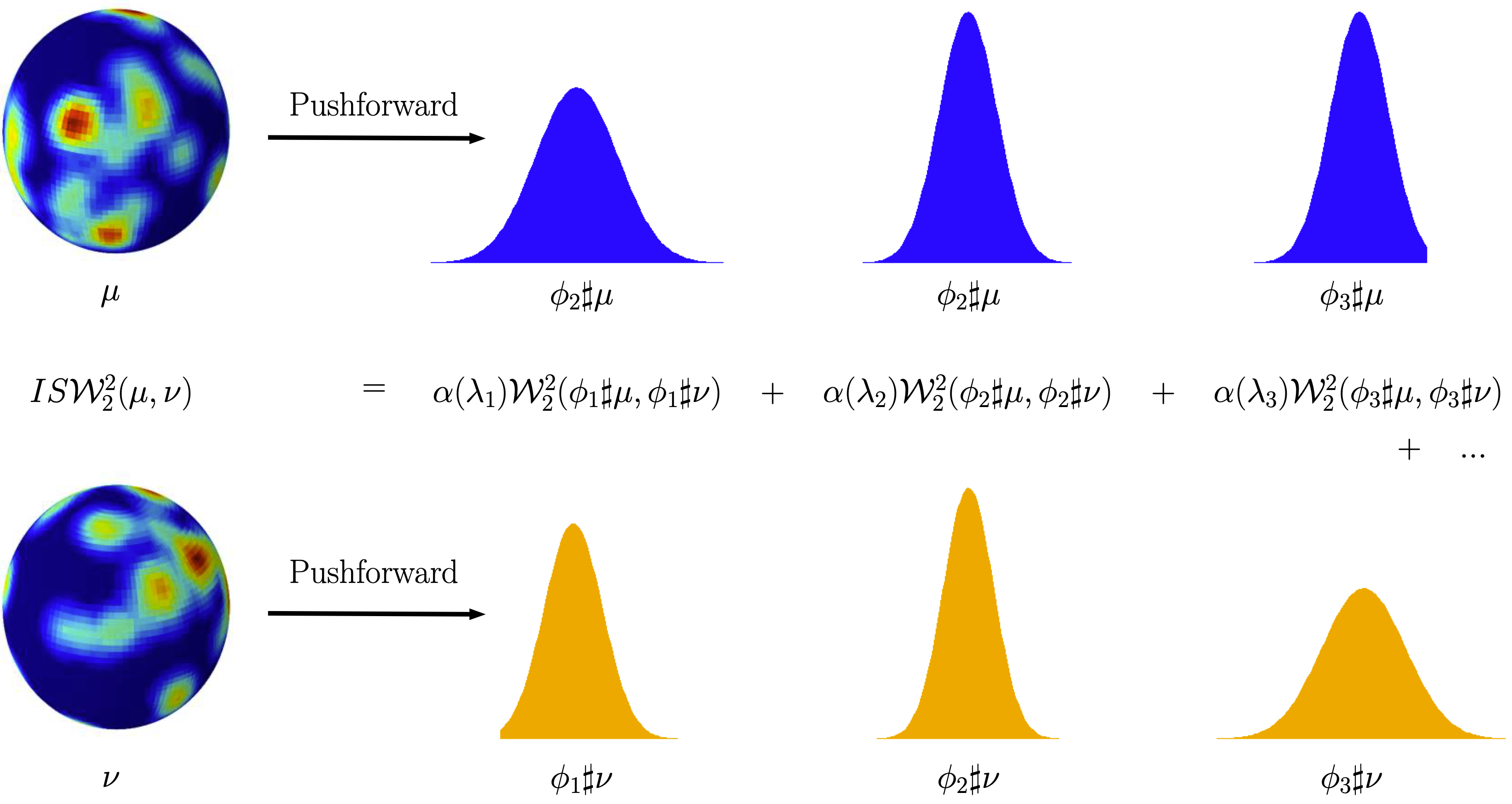
Figure 1: Schematic of the proposed intrinsic slicing construction. Given two probability measures on the sphere (here the darkest blue corresponds to zero mass), different aspects of their dissimilarities become apparent after pushforward to the real line using the eigenfunctions of the Laplace-Beltrami operator, {ϕi}subscriptitalic-ϕ𝑖\{\phi_{i}\}, in this case spherical harmonics. As a particular example of our general construction, the (squared) intrinsic sliced 2-Wasserstein distance IS𝒲22(,)𝐼𝑆superscriptsubscript𝒲22IS\mathcal{W}_{2}^{2}(\cdot,\cdot) is the weighted sum of the dissimilarities of the corresponding pushforwards of μ𝜇\mu and ν𝜈\nu as measured by squared 2-Wasserstein distance 𝒲22(,)superscriptsubscript𝒲22\mathcal{W}_{2}^{2}(\cdot,\cdot) on the real line.

We overcome these difficulties by introducing a new slicing construction on manifolds and graphs (Figure 1) inspired by the sliced 2-Wasserstein (𝒲2subscript𝒲2\mathcal{W}_{2}) distances in high dimensional spaces (Kolouri et al., 2019b, a). Our construction leverages eigenvalues and eigenfunctions/eigenvectors of the Laplace-Beltrami operator on manifolds and Laplacian matrix on graphs to capture the intrinsic geometry and connectivity of the data domain. We apply this slicing construction to obtain a novel class of intrinsic sliced 2-Wasserstein distances on manifolds and graphs. The resulting distances are Hilbert embeddable, have a number of desirable properties, and can be truncated to obtain finite-dimensional embeddings.

Using the corresponding embedding allows us to reduce the distribution collection comparison problem to the comparison of means in a high-dimensional Euclidean space. At the theoretical level our test checks equality of Fréchet means along slicings (see discussion after Example 1 in Section 3.2). These means are transparently tied to the input data, whereby rejections lead to interpretable insights. We provide two approaches for hypothesis testing and verify via extensive experiments that these tests are powerful, and the p𝑝p-values are well-calibrated.

2 Related Work

Our framework is not simply a higher order version of a two-sample kernel test (Gretton et al., 2012) since we test for equality of a specific aspect of meta-distributions. This renders our null hypothesis different from Gretton et al. (2012), and we need a different set of techniques both for proofs and computations. For example, testing in Gretton et al. (2012) can use the permutation null which is valid due to the stronger null hypothesis of equal distributions. In contrast, with our null hypothesis we cannot use the permutation null and have to resort to a bootstrap procedure. Other approaches such as the general Hilbert embedding framework of Petersen & Müller (2016) is not tied to a distance between probability distributions and so can be problematic for capturing the location and variability aspects of distribution collections. In addition, Petersen & Müller (2016) has difficulties in higher dimensions and does not provide constructions suitable for manifolds or graphs.

Sliced Distances

The Sliced Wasserstein (SW) distance and its generalized variant (Kolouri et al., 2019a, GSW) sets up the idea of approximating Wasserstein distances using multiple nonlinear projections, it is presented in extrinsic terms (i.e. Euclidean space) and can suffer from the curse of dimensionality when a low dimensional data manifold lives in a high-dimensional space. Our choice of eigenfunctions for projection is very different from the one-parameter function families in GSW and allows us to rigorously prove a number of general and testing-specific properties.

Moreover, the GSW construction does not directly apply to graphs. While the tree-sliced variant of GSW (Le et al., 2019) can be applied in an intrinsic manner (the clustering variant), it relies on a different type of distance, in the limit related to the euclidean/geodesic distance. This can be seen by comparing our lower bound to theirs: our lower bound for ISW is in terms of the MMD using the spectral distance (Proposition 4.4). The recently-proposed Sobolev transport (Le et al., 2022) does consider measures supported on graphs, but in absence of a slicing construction it is limited to testing for unspecific differences and requires extensive compute due to much slower permutation based calibration (see Section 6). Deshpande et al. (2019) proposed Max Sliced Wasserstein (MSW) distance—taking maximum over projected 𝒲2subscript𝒲2\mathcal{W}_{2} distances vs the average 𝒲2subscript𝒲2\mathcal{W}_{2} distances of SW—in the context of generative models.

Finally, the robust sliced Wasserstein distance of Lai & Zhao (2017) does make use of the geometric properties of the underlying manifold. However, their goal is to compute a correspondence between two manifolds by mapping them into dsuperscript𝑑\mathbb{R}^{d} using eigenmaps and treating the mapped manifolds as measures in dsuperscript𝑑\mathbb{R}^{d} and minimizing some version of Euclidean slicing. None of the aforementioned works consider the problem of comparing collections of distributions, provide ways for obtaining calibrated p𝑝p-values, or prove properties of the distances that make them desirable for hypothesis testing.

3 Preliminaries

3.1 Problem Setup

Given a compact metric space 𝒳𝒳\mathcal{X}, let 𝒫(𝒳)𝒫𝒳\mathcal{P}(\mathcal{X}) denote the set of Borel probability measures on 𝒳𝒳\mathcal{X}. Our main interest is in the case where 𝒳𝒳\mathcal{X} is a graph or a manifold with the shortest/geodesic distance as the metric, and thus the compactness restriction. The 2-Wasserstein distance can be defined on 𝒫(𝒳)𝒫𝒳\mathcal{P}(\mathcal{X}) using the metric of 𝒳𝒳\mathcal{X} as the ground distance (Peyré & Cuturi, 2019; Panaretos & Zemel, 2019), giving 𝒲2𝒳:𝒫(𝒳)×𝒫(𝒳)0:superscriptsubscript𝒲2𝒳𝒫𝒳𝒫𝒳subscriptabsent0\mathcal{W}_{2}^{\mathcal{X}}:\mathcal{P}(\mathcal{X})\times\mathcal{P}(\mathcal{X})\rightarrow\mathbb{R}_{\geq 0}. Due to the repeated use of the real line case we use the shorthand 𝒲2subscript𝒲2\mathcal{W}_{2} when 𝒳=𝒳\mathcal{X}=\mathbb{R}, i.e. 𝒲2:=𝒲2assignsubscript𝒲2superscriptsubscript𝒲2\mathcal{W}_{2}:=\mathcal{W}_{2}^{\mathbb{R}}. Central to our study are distributions on the space of probability measures 𝒫(𝒫(𝒳))=(𝒫(𝒳),(𝒫(𝒳)))𝒫𝒫𝒳𝒫𝒳𝒫𝒳\mathcal{P}(\mathcal{P}(\mathcal{X}))=(\mathcal{P}(\mathcal{X}),\mathcal{B}(\mathcal{P}(\mathcal{X}))), where (𝒫(X))𝒫𝑋\mathcal{B}(\mathcal{P}(X)) is the Borel σ𝜎\sigma-algebra generated by the topology induced by 𝒲2𝒳superscriptsubscript𝒲2𝒳\mathcal{W}_{2}^{\mathcal{X}} (Bigot, 2020). To avoid confusion, we will refer to the elements of 𝒫(𝒫(𝒳))𝒫𝒫𝒳\mathcal{P}(\mathcal{P}(\mathcal{X})) as meta-distributions.

Let P,Q𝒫(𝒫(𝒳))𝑃𝑄𝒫𝒫𝒳P,Q\in\mathcal{P}(\mathcal{P}(\mathcal{X})), and assume that we are given two collections of probability measures {μi}i=1N1superscriptsubscriptsubscript𝜇𝑖𝑖1subscript𝑁1\{\mu_{i}\}_{i=1}^{N_{1}} and {νi}i=1N2superscriptsubscriptsubscript𝜈𝑖𝑖1subscript𝑁2\{\nu_{i}\}_{i=1}^{N_{2}} that are drawn from P𝑃{P} and Q𝑄{Q}: μiPsimilar-tosubscript𝜇𝑖𝑃\mu_{i}\sim{P} and νiQsimilar-tosubscript𝜈𝑖𝑄\nu_{i}\sim{Q} in an independent-and-identically-distributed (hereafter i.i.d.) manner. Our goal is to use this sample to test the null hypothesis of whether P=Q𝑃𝑄P=Q. While this is conceptually a two-sample test, note that our data points are distributions; in practice, the distributions μisubscript𝜇𝑖\mu_{i} or νisubscript𝜈𝑖\nu_{i} are given by histograms.

Remark 3.1.

Let us compare this with the usual two-sample testing. Consider P𝒫(𝒫(𝒳))𝑃𝒫𝒫𝒳P\in\mathcal{P}(\mathcal{P}(\mathcal{X})) constructed as follows. Let μ𝒫(𝒳)superscript𝜇𝒫𝒳\mu^{*}\in\mathcal{P}(\mathcal{X}) be a fixed probability measure. Let x1,x2,xAμsimilar-tosubscript𝑥1subscript𝑥2subscript𝑥𝐴superscript𝜇x_{1},x_{2},...x_{A}\sim\mu^{*} and construct the histogram summarizing this sample: 1Aa=1Aδxa1𝐴superscriptsubscript𝑎1𝐴subscript𝛿subscript𝑥𝑎\frac{1}{A}\sum_{a=1}^{A}\delta_{x_{a}}. Now, 1Aa=1Aδxa𝒫(𝒳)1𝐴superscriptsubscript𝑎1𝐴subscript𝛿subscript𝑥𝑎𝒫𝒳\frac{1}{A}\sum_{a=1}^{A}\delta_{x_{a}}\in\mathcal{P}(\mathcal{X}) is one sample drawn from P𝑃P. Suppose one gets the collection {μi}i=1N1superscriptsubscriptsubscript𝜇𝑖𝑖1subscript𝑁1\{\mu_{i}\}_{i=1}^{N_{1}}, where each histogram is obtained as above: μiPsimilar-tosubscript𝜇𝑖𝑃\mu_{i}\sim P. Similarly, consider Q𝒫(𝒫(𝒳))𝑄𝒫𝒫𝒳Q\in\mathcal{P}(\mathcal{P}(\mathcal{X})) of the same type based on some other fixed ν𝒫(𝒳)superscript𝜈𝒫𝒳\nu^{*}\in\mathcal{P}(\mathcal{X}), and let {νi}i=1N2superscriptsubscriptsubscript𝜈𝑖𝑖1subscript𝑁2\{\nu_{i}\}_{i=1}^{N_{2}} the corresponding collection of histograms. Testing whether P=Q𝑃𝑄P=Q in the limit boils down to μ=νsuperscript𝜇superscript𝜈\mu^{*}=\nu^{*}. When compared to the usual two-sample testing this may seem rather inefficient, requiring A𝐴A times more samples (resp. N1Asubscript𝑁1𝐴N_{1}A and N2Asubscript𝑁2𝐴N_{2}A samples from μsuperscript𝜇\mu^{*} and νsuperscript𝜈\nu^{*}). However, in our general setup it is not assumed that the histograms in the collections come from meta-distributions of the above simple type (i.e. all μisubscript𝜇𝑖\mu_{i} are generated by drawing from the same underlying distribution μsuperscript𝜇\mu^{*}). In fact, the target use-case for our approach is when these histograms are collected by observing different individuals who have their person-specific behaviors/distributions.

Remark 3.2.

To gain further insight into our problem setup, consider it through the lens of statistical manifold theory (Murray & Rice, 1993, SMT). Assume that we observe two collections of parametric distributions: μi=F(x,βi),βiG(β)formulae-sequencesubscript𝜇𝑖𝐹𝑥subscript𝛽𝑖similar-tosubscript𝛽𝑖𝐺𝛽\mu_{i}=F(x,\beta_{i}),\beta_{i}\sim G(\beta) for i=1,,N1𝑖1subscript𝑁1i=1,...,N_{1}, and νi=F(x,γi),γiH(γ)formulae-sequencesubscript𝜈𝑖𝐹𝑥subscript𝛾𝑖similar-tosubscript𝛾𝑖𝐻𝛾\nu_{i}=F(x,\gamma_{i}),\gamma_{i}\sim H(\gamma) for i=1,,N2𝑖1subscript𝑁2i=1,...,N_{2}. Thus, each collection is generated from a distribution of its parameters, resp. G()𝐺G(\cdot) and H()𝐻H(\cdot). The goal of our test is to find out whether G𝐺G and H𝐻H are the same solely by observing the collections {μi}i=1N1superscriptsubscriptsubscript𝜇𝑖𝑖1subscript𝑁1\{\mu_{i}\}_{i=1}^{N_{1}} and {νi}i=1N2superscriptsubscriptsubscript𝜈𝑖𝑖1subscript𝑁2\{\nu_{i}\}_{i=1}^{N_{2}}. While SMT and the Fisher information metric provides a powerful framework for studying parametric families of probability distributions, we focus on more general spaces of probability measures and the Fisher metric may not be easily extended to such nonparametric spaces of measures.

3.2 Hilbert Embeddings

Let 𝒟(,):𝒫(𝒳)×𝒫(𝒳)0:𝒟𝒫𝒳𝒫𝒳subscriptabsent0\mathcal{D}(\cdot,\cdot):\mathcal{P}(\mathcal{X})\times\mathcal{P}(\mathcal{X})\rightarrow\mathbb{R}_{\geq 0} be a distance between probability distributions. 𝒟(,)𝒟\mathcal{D}(\cdot,\cdot) is called Hilbertian (this is just a naming convention; no implication that the map is a Hilbert map) if there exist a Hilbert space \mathcal{H} and a map η:𝒫(𝒳):𝜂𝒫𝒳\eta:\mathcal{P}(\mathcal{X})\rightarrow\mathcal{\mathcal{H}} such that 𝒟(μ,ν)=η(μ)η(ν)𝒟𝜇𝜈subscriptnorm𝜂𝜇𝜂𝜈\mathcal{D}(\mu,\nu)=\|\eta(\mu)-\eta(\nu)\|_{\mathcal{\mathcal{H}}}. For example, it is well-known that 2-Wasserstein distance on 𝒳=𝒳\mathcal{X}=\mathbb{R} is Hilbertian (Peyré & Cuturi, 2019) (also see Section 4.2) and Maximum Mean Discrepancy (MMD) on any 𝒳𝒳\mathcal{X} is Hilbertian (Gretton et al., 2012); however, the 2-Wasserstein distance 𝒲2𝒳superscriptsubscript𝒲2𝒳\mathcal{W}_{2}^{\mathcal{X}} on general 𝒳𝒳\mathcal{X} is not Hilbertian (Peyré & Cuturi, 2019).

Since the map η𝜂\eta takes every measure on 𝒳𝒳\mathcal{X} to a point in \mathcal{H}, we see that a meta-distribution P𝒫(𝒫(𝒳))𝑃𝒫𝒫𝒳P\in\mathcal{P}(\mathcal{P}(\mathcal{X})) gives a rise to a measure on \mathcal{H} given by pushforward operation, η#P=Pη1𝒫()𝜂#𝑃𝑃superscript𝜂1𝒫\eta\#P=P\circ\eta^{-1}\in\mathcal{P}(\mathcal{H}). In addition, if a finite dimensional approximation ηD:𝒫(𝒳)D:subscript𝜂𝐷𝒫𝒳superscript𝐷\eta_{D}:\mathcal{P}(\mathcal{X})\rightarrow\mathbb{R}^{D} of η𝜂\eta is available, then ηD#Psubscript𝜂𝐷#𝑃\eta_{D}\#P is a measure on Dsuperscript𝐷\mathbb{R}^{D}. This observation is enormously useful: problems about the elements of the rather abstract space 𝒫(𝒫(𝒳))𝒫𝒫𝒳\mathcal{P}(\mathcal{P}(\mathcal{X})) are reduced to problems about familiar measures on \mathcal{H} or even Dsuperscript𝐷\mathbb{R}^{D}. For example, the usual notions of mean and variance can be applied to the measure η#P𝜂#𝑃\eta\#P to gain insights about the meta-distribution P𝑃P. The validity of these insights hinges on the η𝜂\eta-map coming from a Hilbertian distance, as distances are central to the statistical quantities of interest.

Testing for η#P=η#Q𝜂#𝑃𝜂#𝑄\eta\#P=\eta\#Q can serve as a proxy for our original testing problem of P=Q𝑃𝑄P=Q. As typical with two-sample tests, various aspects of the equality η#P=η#Q𝜂#𝑃𝜂#𝑄\eta\#P=\eta\#Q can be tested, such as the mean or variance equality; unspecific tests of equality can be applied as well. We will concentrate on testing certain aspects of the equality so that one can easily drill down on the results. This is similar to the regular two-sample testing where checking for equality of, say, means is often preferable as it gives immediately interpretable insights, whereas a general test that only says there are unspecified differences between the distributions is less useful for interpretation. To obtain succint and interpretable tests we concentrate on the mean of the resulting pushforward measure in \mathcal{H}.

Definition 3.3.

For a meta-distribution P𝒫(𝒫(𝒳))𝑃𝒫𝒫𝒳P\in\mathcal{P}(\mathcal{P}(\mathcal{X})), define its Hilbert centroid with respect to the Hilbertian distance 𝒟𝒟\mathcal{D} as Cη#P:=𝔼μP[η(μ)],assignsubscript𝐶𝜂#𝑃subscript𝔼similar-to𝜇𝑃delimited-[]𝜂𝜇C_{\eta\#P}:=\mathbb{E}_{\mu\sim P}[\eta(\mu)]\in\mathcal{H}, assuming it exists.

Our testing procedure is based on checking the equality Cη#P=Cη#Qsubscript𝐶𝜂#𝑃subscript𝐶𝜂#𝑄C_{\eta\#P}=C_{\eta\#Q}, or more explicitly: 𝔼μP[η(μ)]=𝔼νQ[η(ν)]subscript𝔼similar-to𝜇𝑃delimited-[]𝜂𝜇subscript𝔼similar-to𝜈𝑄delimited-[]𝜂𝜈\mathbb{E}_{\mu\sim{P}}[\eta(\mu)]=\mathbb{E}_{\nu\sim{Q}}[\eta(\nu)]. Intuitively, each “dimension” of the map η𝜂\eta probes some aspect of the two involved meta-distributions and makes sure that they are in agreement in expectation. One of our testing approaches will use the statistic

𝕋(P,Q):=Cη#PCη#Q2.assign𝕋𝑃𝑄superscriptsubscriptnormsubscript𝐶𝜂#𝑃subscript𝐶𝜂#𝑄2\mathbb{T}({P},{Q}):=\|C_{\eta\#P}-C_{\eta\#Q}\|_{\mathcal{H}}^{2}. (1)

to capture the deviations from equality; this quantity can be written directly in terms of pairwise distances.

Proposition 3.4.

For P,Q𝒫(𝒫(𝒳))𝑃𝑄𝒫𝒫𝒳P,Q\in\mathcal{P}(\mathcal{P}(\mathcal{X})), the following holds:

𝕋(P,Q)𝕋𝑃𝑄\displaystyle\mathbb{T}({P},{Q}) =𝔼μP,νQ[𝒟2(μ,ν)]absentlimit-fromsubscript𝔼formulae-sequencesimilar-to𝜇𝑃similar-to𝜈𝑄delimited-[]superscript𝒟2𝜇𝜈\displaystyle=\mathbb{E}_{\mu\sim{P},\nu\sim{Q}}[\mathcal{D}^{2}(\mu,\nu)]-
12𝔼μ,μP[𝒟2(μ,μ)]12𝔼ν,νQ[𝒟2(ν,ν)].12subscript𝔼similar-to𝜇superscript𝜇𝑃delimited-[]superscript𝒟2𝜇superscript𝜇12subscript𝔼similar-to𝜈superscript𝜈𝑄delimited-[]superscript𝒟2𝜈superscript𝜈\displaystyle\frac{1}{2}\mathbb{E}_{\mu,\mu^{\prime}\sim{P}}[\mathcal{D}^{2}(\mu,\mu^{\prime})]-\frac{1}{2}\mathbb{E}_{\nu,\nu^{\prime}\sim{Q}}[\mathcal{D}^{2}(\nu,\nu^{\prime})].

Next we give an example of what Hilbert centroid equality implies in an important special case.

Example 1.

Let 𝒳=[0,T]𝒳0𝑇\mathcal{X}=[0,T]\subset\mathbb{R} with 𝒟𝒟\mathcal{D} being the 2-Wasserstein distance 𝒲2subscript𝒲2\mathcal{W}_{2}. Given a probability measure μ𝒫([0,T])𝜇𝒫0𝑇\mu\in\mathrm{\mathcal{P}}([0,T]), let Fμsubscript𝐹𝜇F_{\mu} be its cumulative distribution function: Fμ(x)=μ([0,x])=0x𝑑μsubscript𝐹𝜇𝑥𝜇0𝑥superscriptsubscript0𝑥differential-d𝜇F_{\mu}(x)=\mu([0,x])=\int_{0}^{x}d\mu. The generalized inverse of cumulative distribution function (CDF) is defined by Fμ1(s):=inf{x[0,T]:Fμ(x)>s}assignsuperscriptsubscript𝐹𝜇1𝑠infimumconditional-set𝑥0𝑇subscript𝐹𝜇𝑥𝑠F_{\mu}^{-1}(s):=\inf\{x\in[0,T]:F_{\mu}(x)>s\}. The squared 2-Wasserstein distance has a rather simple expression in terms of the inverse CDF (Peyré & Cuturi, 2019):

𝒲22(μ,ν)=01(Fμ1(s)Fν1(s))2𝑑s.superscriptsubscript𝒲22𝜇𝜈superscriptsubscript01superscriptsuperscriptsubscript𝐹𝜇1𝑠superscriptsubscript𝐹𝜈1𝑠2differential-d𝑠\mathcal{W}_{2}^{2}(\mu,\nu)=\int_{0}^{1}(F_{\mu}^{-1}(s)-F_{\nu}^{-1}(s))^{2}ds. (2)

This formula immediately establishes the Hilbertianity of 𝒲2subscript𝒲2\mathcal{W}_{2} through the map η:𝒫([0,T])L2([0,T]):𝜂𝒫0𝑇subscript𝐿20𝑇\eta:\mathcal{P}([0,T])\rightarrow L_{2}([0,T]) defined by η(μ)=Fμ1𝜂𝜇superscriptsubscript𝐹𝜇1\eta(\mu)=F_{\mu}^{-1}. Note that η𝜂\eta is invertible for increasing normalized functions in the embedding space. Using this insight, we see that the corresponding “average measure” of P𝒫(𝒫(𝒳))𝑃𝒫𝒫𝒳P\in\mathcal{P}(\mathcal{P}(\mathcal{X})) can be introduced via Pav=η1(𝔼μP[η(μ)])subscript𝑃avsuperscript𝜂1subscript𝔼similar-to𝜇𝑃delimited-[]𝜂𝜇{P}_{\mathrm{av}}=\eta^{-1}(\mathbb{E}_{\mu\sim{P}}[\eta(\mu)]). It is easy to prove that Pavsubscript𝑃av{P}_{\mathrm{av}} satisfies the following: Pav=argminρ𝒫(𝒳)𝔼μP[𝒲2(μ,ρ)2]subscript𝑃avsubscript𝜌𝒫𝒳subscript𝔼similar-to𝜇𝑃delimited-[]subscript𝒲2superscript𝜇𝜌2{P}_{\mathrm{av}}=\arg\min_{\rho\in\mathcal{P}(\mathcal{X})}\mathbb{E}_{\mu\sim{P}}[\mathcal{W}_{2}(\mu,\rho)^{2}], which is the definition of the Fréchet mean, see for example (Peyré & Cuturi, 2019). In this setting, Cη#P=Cη#Qsubscript𝐶𝜂#𝑃subscript𝐶𝜂#𝑄C_{\eta\#P}=C_{\eta\#Q} boils down to having the same Fréchet means, Pav=Qavsubscript𝑃avsubscript𝑄av{P}_{\mathrm{av}}={Q}_{\mathrm{av}}.

We will later see that the Hilbert embedding corresponding to the intrinsic sliced 2-Wasserstein distance is assembled of embeddings like in Example 1 applied after pushforwards (see Figure 1 for an intuition). This means that the resulting equality Cη#P=Cη#Qsubscript𝐶𝜂#𝑃subscript𝐶𝜂#𝑄C_{\eta\#P}=C_{\eta\#Q} becomes more stringent, making it a better proxy for detecting the deviations from P=Q𝑃𝑄P=Q without losing the interpretability aspect.

4 Intrinsic Sliced 2-Wasserstein Distance

We introduce a Hilbertian version of 𝒲2subscript𝒲2\mathcal{W}_{2} on manifolds and graphs via a construction we call intrinsic slicing due to its use of the domain’s intrinsic geometric properties. To focus our discussion we concentrate on the manifold case, as the graph case is simpler and is obtained by replacing the Laplace-Beltrami operator by the graph Laplacian.

Let λ,ϕ;=0,1,.formulae-sequencesubscript𝜆subscriptitalic-ϕ01\lambda_{\ell},\phi_{\ell};\ell=0,1,.... be the eigenvalues and eigenfunctions of the Laplace-Beltrami operator on 𝒳𝒳\mathcal{X} with Neumann boundary conditions. The eigenfunctions are sorted by increasing eignevalue and assumed to be orthonormal with respect to some fixed (e.g. uniform) measure on 𝒳𝒳\mathcal{X}; also ϕ0=constsubscriptitalic-ϕ0𝑐𝑜𝑛𝑠𝑡\phi_{0}=const and λ0=0subscript𝜆00\lambda_{0}=0. One can define the spectral kernel k(x,y)=α(λ)ϕ(x)ϕ(y)𝑘𝑥𝑦subscript𝛼subscript𝜆subscriptitalic-ϕ𝑥subscriptitalic-ϕ𝑦k(x,y)=\sum_{\ell}\alpha(\lambda_{\ell})\phi_{\ell}(x)\phi_{\ell}(y) and the corresponding spectral distance on the manifold d(x,y)=k(x,x)+k(y,y)2k(x,y)=α(λ)(ϕ(x)ϕ(y))2𝑑𝑥𝑦𝑘𝑥𝑥𝑘𝑦𝑦2𝑘𝑥𝑦𝛼subscript𝜆superscriptsubscriptitalic-ϕ𝑥subscriptitalic-ϕ𝑦2d(x,y)=k(x,x)+k(y,y)-2k(x,y)=\sum\alpha(\lambda_{\ell})(\phi_{\ell}(x)-\phi_{\ell}(y))^{2}, where α:00:𝛼subscriptabsent0subscriptabsent0\alpha:\mathbb{R}_{\geq 0}\rightarrow\mathbb{R}_{\geq 0} is a function that controls contribution from each spectral band. By setting α(λ)=etλ𝛼𝜆superscript𝑒𝑡𝜆\alpha(\lambda)=e^{-t\lambda} for some t>0𝑡0t>0, we get the heat/diffusion kernel and the corresponding diffusion distance (Coifman & Lafon, 2006). Another important case is α(λ)=1/λ2𝛼𝜆1superscript𝜆2\alpha(\lambda)=1/\lambda^{2} if λ>0𝜆0\lambda>0 and α(0)=0𝛼00\alpha(0)=0, which gives the biharmonic kernel and distance (Lipman et al., 2010). In both of these constructions α()𝛼\alpha(\cdot) is a decreasing function, allowing the smoother low-frequency (i.e. smaller λsubscript𝜆\lambda_{\ell}) eigenfunctions to contribute more.

4.1 Definition and properties

A real-valued function ϕ:𝒳:italic-ϕ𝒳\phi:\mathcal{X}\rightarrow\mathbb{R} can be used to map the manifold 𝒳𝒳\mathcal{X} onto the real line. Any probability measure μ𝒫(𝒳)𝜇𝒫𝒳\mu\in\mathcal{P}(\mathcal{X}) can likewise be projected onto the real line using the pushforward of ϕitalic-ϕ\phi, which we denote by ϕμ=μϕ1𝒫()italic-ϕ𝜇𝜇superscriptitalic-ϕ1𝒫\phi\sharp\mu=\mu\circ\phi^{-1}\in\mathcal{P}(\mathbb{R}). While the pushforward notions used here and in previous sections are conceptually the same, for clarity we use \sharp for measures and ##\# for meta-distributions. We define intrinsic slicing as follows.

Definition 4.1.

Given a function α:00:𝛼subscriptabsent0subscriptabsent0\alpha:\mathbb{R}_{\geq 0}\rightarrow\mathbb{R}_{\geq 0} and a probability distance 𝒟(,)𝒟\mathcal{D}(\cdot,\cdot) on 𝒫()𝒫\mathcal{P}(\mathbb{R}), we define the intrinsic sliced distance IS𝒟(,)𝐼𝑆𝒟IS\mathcal{D}(\cdot,\cdot) on 𝒫(𝒳)𝒫𝒳\mathcal{P}(\mathcal{X}) by

IS𝒟2(μ,ν)=α(λ)𝒟2(ϕμ,ϕν).𝐼𝑆superscript𝒟2𝜇𝜈subscript𝛼subscript𝜆superscript𝒟2subscriptitalic-ϕ𝜇subscriptitalic-ϕ𝜈IS\mathcal{D}^{2}(\mu,\nu)=\sum_{\ell}\alpha(\lambda_{\ell})\mathcal{D}^{2}(\phi_{\ell}\sharp\mu,\phi_{\ell}\sharp\nu).

The choice of the Laplacian eigenfunctions in the definition can be justified by a number of their properties. Eigenfunctions are intrinsic quantities of a manifold and are ordered by smoothness. Thus, they allow capturing the intrinsic connectivity of the underlying domain. Furthermore, due to the orthogonality of eigenfunctions, their pushforwards can capture complementary aspects of the distribution.

While the definition is general, our focus in this paper is on the case when 𝒟=𝒲2𝒟subscript𝒲2\mathcal{D}=\mathcal{W}_{2}; we remind that we always use 𝒲2subscript𝒲2\mathcal{W}_{2} to denote the 2-Wasserstein distance on 𝒫()𝒫\mathcal{P}(\mathbb{R}). We call the resulting distance Intrinsic Sliced 2-Wasserstein Distance, and denote it by IS𝒲2𝐼𝑆subscript𝒲2IS\mathcal{W}_{2}. First, we discuss the convergence of the infinite sum in Definition 4.1.

Proposition 4.2.

If 𝒳𝒳\mathcal{X} is a smooth compact n𝑛n-dimensional manifold and λ(n1)/2α(λ)<subscriptsuperscriptsubscript𝜆𝑛12𝛼subscript𝜆\sum_{\ell}\lambda_{\ell}^{(n-1)/2}\alpha(\lambda_{\ell})<\infty, then IS𝒲2𝐼𝑆subscript𝒲2IS\mathcal{W}_{2} is well-defined.

Next, we prove a number of properties of IS𝒟𝐼𝑆𝒟IS\mathcal{D}.

Proposition 4.3.

If 𝒟𝒟\mathcal{D} is a Hilbertian probability distance such that IS𝒟𝐼𝑆𝒟IS\mathcal{D} is well-defined, then (i) IS𝒟𝐼𝑆𝒟IS\mathcal{D} is Hilbertian, and (ii) IS𝒟𝐼𝑆𝒟IS\mathcal{D} satisfies the following metric properties: non-negativity, symmetry, the triangle inequality, and IS𝒟(μ,μ)=0𝐼𝑆𝒟𝜇𝜇0IS\mathcal{D}(\mu,\mu)=0.

Proof.

By Hilbertian property of 𝒟𝒟\mathcal{D}, there exists a Hilbert space 0superscript0\mathcal{H}^{0} and a map η0:𝒫()0:superscript𝜂0𝒫superscript0\eta^{0}:\mathcal{P}(\mathbb{R})\rightarrow\mathcal{H}^{0} such that 𝒟(ρ1,ρ2)=η0(ρ1)η0(ρ2)0𝒟subscript𝜌1subscript𝜌2subscriptnormsuperscript𝜂0subscript𝜌1superscript𝜂0subscript𝜌2superscript0\mathcal{D}(\rho_{1},\rho_{2})=\|\eta^{0}(\rho_{1})-\eta^{0}(\rho_{2})\|_{\mathcal{\mathcal{H}^{0}}} for all ρ1,ρ2𝒫()subscript𝜌1subscript𝜌2𝒫\rho_{1},\rho_{2}\in\mathcal{P}(\mathbb{R}). Plugging this into Definition 4.1 we have IS𝒟(μ,ν)=η(μ)η(ν)𝐼𝑆𝒟𝜇𝜈subscriptnorm𝜂𝜇𝜂𝜈IS\mathcal{D}(\mu,\nu)=\|\eta(\mu)-\eta(\nu)\|_{\mathcal{\mathcal{H}}}, where =0subscriptdirect-sumsuperscript0\mathcal{H}=\oplus_{\ell}\mathcal{H}^{0} and the \ell-th component of η(μ)𝜂𝜇\eta(\mu) is α(λ)η0(ϕμ)𝛼subscript𝜆subscript𝜂0subscriptitalic-ϕ𝜇\sqrt{\alpha(\lambda_{\ell})}\eta_{0}(\phi_{\ell}\sharp\mu)\in\mathcal{H}. The second part of Proposition 4.3 directly follows from the Hilbert property. ∎

Since 𝒲2subscript𝒲2\mathcal{W}_{2} is Hilbertian on 𝒫()𝒫\mathcal{P}(\mathbb{R}), the application of Proposition 4.3 yields that IS𝒲2𝐼𝑆subscript𝒲2IS\mathcal{W}_{2} is also Hilberitan, making it possible to use IS𝒲2𝐼𝑆subscript𝒲2IS\mathcal{W}_{2} for our hypothesis tests in Section 5.

For a simple choice of distance 𝒟𝒟\mathcal{D} on 𝒫()𝒫\mathcal{P}(\mathbb{R}), namely the absolute mean difference, the corresponding intrinsic sliced distance is the well-known MMD (Gretton et al., 2012).

Proposition 4.4.

Let 𝒟(ρ1,ρ2)=|𝔼xρ1[x]𝔼yρ2[y]|𝒟subscript𝜌1subscript𝜌2subscript𝔼similar-to𝑥subscript𝜌1delimited-[]𝑥subscript𝔼similar-to𝑦subscript𝜌2delimited-[]𝑦\mathcal{D}(\rho_{1},\rho_{2})=|\mathbb{E}_{x\sim\rho_{1}}[x]-\mathbb{E}_{y\sim\rho_{2}}[y]| for ρ1,ρ2𝒫()subscript𝜌1subscript𝜌2𝒫\rho_{1},\rho_{2}\in\mathcal{P}(\mathbb{R}), then the corresponding IS𝒟𝐼𝑆𝒟IS\mathcal{D} is equivalent to the MMD with the spectral kernel k(,)𝑘k(\cdot,\cdot).

When k(x,y)𝑘𝑥𝑦k(x,y) is the heat kernel, the sliced distance in Proposition 4.4 is very much like the MMD with the Gaussian kernel, with the parameter t𝑡t in α(λ)=etλ𝛼𝜆superscript𝑒𝑡𝜆\alpha(\lambda)=e^{-t\lambda} controlling the kernel width. Indeed, the two kernels coincide on dsuperscript𝑑\mathbb{R}^{d}, and on general manifolds Varadhan’s formula gives asymptotic equivalence for small t𝑡t (Berger, 2003).

An interesting insight derived from the above result is that IS𝒲2𝐼𝑆subscript𝒲2IS\mathcal{W}_{2} is in a sense a “stronger” distance than MMD that uses the corresponding spectral kernel. The IS𝒲2𝐼𝑆subscript𝒲2IS\mathcal{W}_{2} compares the quantiles of the pushforward distributions (Eq. (2)), whereas MMD compares their expectations only. We formalize this notion in the next result, also providing a theoretical reason for preferring IS𝒲2𝐼𝑆subscript𝒲2IS\mathcal{W}_{2} for hypothesis testing.

Proposition 4.5.

MMD(μ,ν)IS𝒲2(μ,ν)𝑀𝑀𝐷𝜇𝜈𝐼𝑆subscript𝒲2𝜇𝜈MMD(\mu,\nu)\leq IS\mathcal{W}_{2}(\mu,\nu) when the same α()𝛼\alpha(\cdot) is used in both constructions.

We are now in a position to prove that IS𝒲2𝐼𝑆subscript𝒲2IS\mathcal{W}_{2} is a true metric.

Theorem 4.6.

If α(λ)>0𝛼𝜆0\alpha(\lambda)>0 for all λ>0𝜆0\lambda>0 , then IS𝒲2𝐼𝑆subscript𝒲2IS\mathcal{W}_{2} is a metric on 𝒫(𝒳)𝒫𝒳\mathcal{P}(\mathcal{X}).

We remind that 2-Wasserstein distance can be defined directly on 𝒫(𝒳)𝒫𝒳\mathcal{P}(\mathcal{X}) using the geodesic distance as the ground metric; we denote this distance as 𝒲2𝒳superscriptsubscript𝒲2𝒳\mathcal{W}_{2}^{\mathcal{X}}. Lipschitz properties of the eigenfunctions imply the following:

Proposition 4.7.

There exists a constant c𝑐c depending only on 𝒳n𝒳superscript𝑛\mathcal{X}\subseteq\mathbb{R}^{n} such that for all μ,ν𝒫(𝒳)𝜇𝜈𝒫𝒳\mu,\nu\in\mathcal{P}(\mathcal{X}) the inequality IS𝒲2(μ,ν)c𝒲2𝒳(μ,ν)λ(n+3)/2α(λ)𝐼𝑆subscript𝒲2𝜇𝜈𝑐superscriptsubscript𝒲2𝒳𝜇𝜈subscriptsuperscriptsubscript𝜆𝑛32𝛼subscript𝜆IS\mathcal{W}_{2}(\mu,\nu)\leq c\mathcal{W}_{2}^{\mathcal{X}}(\mu,\nu)\sqrt{\sum_{\ell}\lambda_{\ell}^{(n+3)/2}\alpha(\lambda_{\ell})} holds.

Our final result looks at the quantity 𝕋𝕋\mathbb{T} defined using IS𝒲2𝐼𝑆subscript𝒲2IS\mathcal{W}_{2} by Eq. (1). We will be using 𝕋𝕋\mathbb{T} computed on finite collections of measures as a test statistic in the next section. We show that it enjoys robustness with respect to small perturbations of the measures in the collection.

Proposition 4.8.

Let {μi}i=1Nsuperscriptsubscriptsubscript𝜇𝑖𝑖1𝑁\{\mu_{i}\}_{i=1}^{N} and {νi}i=1Nsuperscriptsubscriptsubscript𝜈𝑖𝑖1𝑁\{\nu_{i}\}_{i=1}^{N} be two collections of probability measures on 𝒫(𝒳)𝒫𝒳\mathcal{P}(\mathcal{X}), such that i,𝒲2𝒳(μi,νi)ϵfor-all𝑖superscriptsubscript𝒲2𝒳subscript𝜇𝑖subscript𝜈𝑖italic-ϵ\forall i,\mathcal{W}_{2}^{\mathcal{X}}(\mu_{i},\nu_{i})\leq\epsilon, then 𝕋({μi}i=1N,{νi}i=1N)C2ϵ2𝕋superscriptsubscriptsubscript𝜇𝑖𝑖1𝑁superscriptsubscriptsubscript𝜈𝑖𝑖1𝑁superscript𝐶2superscriptitalic-ϵ2\mathbb{T}(\{\mu_{i}\}_{i=1}^{N},\{\nu_{i}\}_{i=1}^{N})\leq C^{2}\epsilon^{2}. Here C=cλ(n+3)/2α(λ)𝐶𝑐subscriptsuperscriptsubscript𝜆𝑛32𝛼subscript𝜆C=c\sqrt{\sum_{\ell}\lambda_{\ell}^{(n+3)/2}\alpha(\lambda_{\ell})} from previous proposition and is assumed to be finite.

This bound implies that if the distributions in a collection undergo horizontal shifts that are small as measured by the geodesic distance 𝒲2𝒳superscriptsubscript𝒲2𝒳\mathcal{W}_{2}^{\mathcal{X}} , then 𝕋𝕋\mathbb{T} is small as well.

4.2 Approximate Hilbert Embedding

An important aspect of IS𝒲2𝐼𝑆subscript𝒲2IS\mathcal{W}_{2} is that its Hilbert map η:𝒫(𝒳):𝜂𝒫𝒳\eta:\mathcal{P}(\mathcal{X})\rightarrow\mathcal{\mathcal{H}} can be approximated by a finite-dimensional embedding ηD:𝒫(𝒳)D:subscript𝜂𝐷𝒫𝒳superscript𝐷\eta_{D}:\mathcal{P}(\mathcal{X})\rightarrow\mathbb{R}^{D} such that IS𝒲2(μ,ν)ηD(μ)ηD(ν)D𝐼𝑆subscript𝒲2𝜇𝜈subscriptnormsubscript𝜂𝐷𝜇subscript𝜂𝐷𝜈superscript𝐷IS\mathcal{W}_{2}(\mu,\nu)\approx\|\eta_{D}(\mu)-\eta_{D}(\nu)\|_{\mathbb{R}^{D}}. This is useful for practical computation and for one of our hypothesis testing approaches.

Using the formula for IS𝒲2𝐼𝑆subscript𝒲2IS\mathcal{W}_{2} on 𝒫()𝒫\mathcal{P}(\mathbb{R}) in terms of the quantile function, Eq. (2), the Hilbert map is defined by η0(μ)=Fμ1superscript𝜂0𝜇superscriptsubscript𝐹𝜇1\eta^{0}(\mu)=F_{\mu}^{-1}. We have 𝒲2(μ,ν)=η0(μ)η0(ν)L2()subscript𝒲2𝜇𝜈subscriptnormsuperscript𝜂0𝜇superscript𝜂0𝜈subscript𝐿2\mathcal{W}_{2}(\mu,\nu)=\|\eta^{0}(\mu)-\eta^{0}(\nu)\|_{L_{2}(\mathbb{R})}, where the norm involves integration. We can discretize the integral using the Riemann sum for equidistant knots sk=k1D,k=1,,Dformulae-sequencesubscript𝑠𝑘𝑘1superscript𝐷𝑘1superscript𝐷s_{k}=\frac{k-1}{D^{\prime}},k=1,...,D^{\prime}, define the approximate embedding ηD0:𝒫()D:superscriptsubscript𝜂superscript𝐷0𝒫superscriptsuperscript𝐷\eta_{D^{\prime}}^{0}:\mathcal{P}(\mathbb{R})\rightarrow\mathbb{R}^{D^{\prime}} as:

ηD0:μ1D[Fμ1(s1),,Fμ1(sD)].:superscriptsubscript𝜂superscript𝐷0𝜇1superscript𝐷superscriptsubscript𝐹𝜇1subscript𝑠1superscriptsubscript𝐹𝜇1subscript𝑠superscript𝐷\eta_{D^{\prime}}^{0}:\mu\rightarrow\frac{1}{\sqrt{D^{\prime}}}[F_{\mu}^{-1}(s_{1}),...,F_{\mu}^{-1}(s_{D^{\prime}})]. (3)

Now, 𝒲2(μ,ν)ηD0(μ)ηD0(ν)Dsubscript𝒲2𝜇𝜈subscriptnormsuperscriptsubscript𝜂superscript𝐷0𝜇superscriptsubscript𝜂superscript𝐷0𝜈superscriptsuperscript𝐷\mathcal{W}_{2}(\mu,\nu)\approx\|\eta_{D^{\prime}}^{0}(\mu)-\eta_{D^{\prime}}^{0}(\nu)\|_{\mathbb{R}^{D^{\prime}}} with approximation quality depending on the embedding dimension Dsuperscript𝐷D^{\prime}.

To approximate the Hilbert map for IS𝒲2𝐼𝑆subscript𝒲2IS\mathcal{W}_{2} we truncate the series defining IS𝒲2𝐼𝑆subscript𝒲2IS\mathcal{W}_{2} and use a finite number of eigenfunctions for pushforward: ϕ,=1,,Lformulae-sequencesubscriptitalic-ϕ1𝐿\phi_{\ell},\ell=1,...,L, where ϕ0subscriptitalic-ϕ0\phi_{0} is dropped since it is a constant. By inspecting the proof of Proposition 4.3 and using Eq. (3), we can define ηD:𝒫(𝒳)D:subscript𝜂𝐷𝒫𝒳superscript𝐷\eta_{D}:\mathcal{P}(\mathcal{X})\rightarrow\mathbb{R}^{D} with D=LD𝐷𝐿superscript𝐷D=LD^{\prime} as the concatenation of L𝐿L maps:

(ηD):μα(λ)D[Fϕμ1(s1),,Fϕμ1(sD)].:subscriptsubscript𝜂𝐷𝜇𝛼subscript𝜆superscript𝐷superscriptsubscript𝐹subscriptitalic-ϕ𝜇1subscript𝑠1superscriptsubscript𝐹subscriptitalic-ϕ𝜇1subscript𝑠superscript𝐷(\eta_{D})_{\ell}:\mu\rightarrow\sqrt{\frac{\alpha(\lambda_{\ell})}{D^{\prime}}}[F_{\phi_{\ell}\sharp\mu}^{-1}(s_{1}),...,F_{\phi_{\ell}\sharp\mu}^{-1}(s_{D^{\prime}})].

Spectral decompositions of Laplace-Beltrami operators for general manifolds (Coifman & Lafon, 2006; Reuter et al., 2009) or graph Laplacians can be computed numerically. For applications involving simple manifolds, eigenvalues and eigenfunctions can be computed analytically (see Appendix A.3).

The hyperparameters L𝐿L and Dsuperscript𝐷D^{\prime} capture distinct aspects of the complexity of the distribution. A larger L𝐿L allows access to higher order eigenfunctions that possess greater spatial oscillations, linking to the finer details of the geometry and topology of the underlying domain and distribution collection. On the other hand, Dsuperscript𝐷D^{\prime} captures how well the pushforward distribution is represented, which is determined by the number of quantiles. Both hyperparameters can have a significant impact on the success of the testing process.

5 Hypothesis Testing

Let {μi}i=1N1superscriptsubscriptsubscript𝜇𝑖𝑖1subscript𝑁1\{\mu_{i}\}_{i=1}^{N_{1}} and {νi}i=1N2superscriptsubscriptsubscript𝜈𝑖𝑖1subscript𝑁2\{\nu_{i}\}_{i=1}^{N_{2}} be two i.i.d. collections of measures drawn from P,Q𝒫(𝒫(𝒳))𝑃𝑄𝒫𝒫𝒳P,Q\in\mathcal{P}(\mathcal{P}(\mathcal{X})) respectively. Our goal is to use these samples to test the null hypothesis H0:Cη#P=Cη#Q:subscript𝐻0subscript𝐶𝜂#𝑃subscript𝐶𝜂#𝑄H_{0}:C_{\eta\#P}=C_{\eta\#Q}, where η𝜂\eta is the Hilbert embedding of the sliced distance IS𝒲2𝐼𝑆subscript𝒲2IS\mathcal{W}_{2} on 𝒫(𝒳)𝒫𝒳\mathcal{P}(\mathcal{X}).

5.1 Resampling Based Test

We use the quantity 𝕋(,)𝕋\mathbb{T}(\cdot,\cdot) from Eq. (1) as the test statistic. Its sample version is computed by replacing the expectations by the empirical means, and excluding the diagonal terms to achieve unbiasedness

𝕋^^𝕋absent\displaystyle\hat{\mathbb{T}}\equiv i,j:ijIS𝒲22(μi,μj)2N1(N11)+i,j:ijIS𝒲22(νi,νj)2N2(N21)subscript:𝑖𝑗𝑖𝑗𝐼𝑆superscriptsubscript𝒲22subscript𝜇𝑖subscript𝜇𝑗2subscript𝑁1subscript𝑁11subscript:𝑖𝑗𝑖𝑗𝐼𝑆superscriptsubscript𝒲22subscript𝜈𝑖subscript𝜈𝑗2subscript𝑁2subscript𝑁21\displaystyle\sum_{i,j:i\neq j}\frac{IS\mathcal{W}_{2}^{2}(\mu_{i},\mu_{j})}{2N_{1}(N_{1}-1)}+\sum_{i,j:i\neq j}\frac{IS\mathcal{W}_{2}^{2}(\nu_{i},\nu_{j})}{2N_{2}(N_{2}-1)} (4)
i,jIS𝒲22(μi,νj)N1N2.subscript𝑖𝑗𝐼𝑆superscriptsubscript𝒲22subscript𝜇𝑖subscript𝜈𝑗subscript𝑁1subscript𝑁2\displaystyle-\sum_{i,j}\frac{IS\mathcal{W}_{2}^{2}(\mu_{i},\nu_{j})}{N_{1}N_{2}}.

Note that 𝔼𝕋^=𝕋(P,Q)𝔼^𝕋𝕋𝑃𝑄\mathbb{E}\hat{\mathbb{T}}=\mathbb{T}({P},{Q}). In practice, the IS𝒲2𝐼𝑆subscript𝒲2IS\mathcal{W}_{2} values are computed from the approximate embedding: IS𝒲2(ρ1,ρ2)ηD(ρ1)ηD(ρ2)D𝐼𝑆subscript𝒲2subscript𝜌1subscript𝜌2subscriptnormsubscript𝜂𝐷subscript𝜌1subscript𝜂𝐷subscript𝜌2superscript𝐷IS\mathcal{W}_{2}(\rho_{1},\rho_{2})\approx\|\eta_{D}(\rho_{1})-\eta_{D}(\rho_{2})\|_{\mathbb{R}^{D}}. We denote the resulting statistic by 𝕋~L,Dsubscript~𝕋𝐿superscript𝐷\tilde{\mathbb{T}}_{L,D^{\prime}}.

The difference between 𝕋~L,Dsubscript~𝕋𝐿superscript𝐷\tilde{\mathbb{T}}_{L,D^{\prime}} and the population version (i.e. 𝕋𝕋~L,D𝕋subscript~𝕋𝐿superscript𝐷\mathbb{T}-\tilde{\mathbb{T}}_{L,D^{\prime}}) can be decomposed as (𝕋𝕋^)+(𝕋^𝕋^L)+(𝕋^L𝕋~L,D)𝕋^𝕋^𝕋subscript^𝕋𝐿subscript^𝕋𝐿subscript~𝕋𝐿superscript𝐷(\mathbb{T}-\hat{\mathbb{T}})+(\mathbb{\hat{T}}-\hat{\mathbb{T}}_{L})+(\hat{\mathbb{T}}_{L}-\tilde{\mathbb{T}}_{L,D^{\prime}}), where the summands inside the terms 𝕋^Lsubscript^𝕋𝐿\hat{\mathbb{T}}_{L} and 𝕋~L,Dsubscript~𝕋𝐿superscript𝐷\tilde{\mathbb{T}}_{L,D^{\prime}} correspond to partial sums that approximate IS𝒲22(,)𝐼𝑆superscriptsubscript𝒲22IS\mathcal{W}_{2}^{2}(\cdot,\cdot) by l=1Lα(λl)𝒲22(ϕl,ϕl)\sum_{l=1}^{L}\alpha(\lambda_{l})\mathcal{W}_{2}^{2}(\phi_{l}\sharp\cdot,\phi_{l}\sharp\cdot), and 𝒲22(ϕl,ϕl)\mathcal{W}_{2}^{2}(\phi_{l}\sharp\cdot,\phi_{l}\sharp\cdot) by ηD(ϕl)ηD(ϕl)2\|\eta_{D^{\prime}}(\phi_{l}\sharp\cdot)-\eta_{D^{\prime}}(\phi_{l}\sharp\cdot)\|^{2}, respectively. We show in Appendix A.4 that a) summands in the second and third terms in the sum can be made infinitesmally small by choosing large enough L𝐿L and Dsuperscript𝐷D^{\prime}, respectively; b) an asymptotic result for the first difference can be obtained by extending the tools from Gretton et al. (2012); Serfling (2009). These results are based on several assumptions detailed in Appendix A.4. Combining the two results, we establish asymptotic distributions of 𝕋~L,Dsubscript~𝕋𝐿superscript𝐷\tilde{\mathbb{T}}_{L,D^{\prime}}:

Theorem 5.1.

Assume relevant conditions (see Appendix A.4) hold. Define N=N1+N2𝑁subscript𝑁1subscript𝑁2N=N_{1}+N_{2}, and suppose that as N1,N2subscript𝑁1subscript𝑁2N_{1},N_{2}\rightarrow\infty, we have N1/Nρ1,N2/Nρ2=1ρ1formulae-sequencesubscript𝑁1𝑁subscript𝜌1subscript𝑁2𝑁subscript𝜌21subscript𝜌1N_{1}/N\rightarrow\rho_{1},N_{2}/N\rightarrow\rho_{2}=1-\rho_{1}, for some fixed 0<ρ1<10subscript𝜌110<\rho_{1}<1.With LLN,DDNformulae-sequence𝐿subscript𝐿𝑁superscript𝐷subscript𝐷𝑁L\geq L_{N},D^{\prime}\geq D_{N} chosen in an appropriate way (see Appendix A.4), under H0:Cη#P=Cη#Q:subscript𝐻0subscript𝐶𝜂#𝑃subscript𝐶𝜂#𝑄H_{0}:C_{\eta\#P}=C_{\eta\#Q} we have

N𝕋~L,Dm=1γm(Am21),𝑁subscript~𝕋𝐿superscript𝐷superscriptsubscript𝑚1subscript𝛾𝑚superscriptsubscript𝐴𝑚21N\tilde{\mathbb{T}}_{L,D^{\prime}}\leadsto\sum_{m=1}^{\infty}\gamma_{m}(A_{m}^{2}-1),

where AmN(0,1)similar-tosubscript𝐴𝑚𝑁01A_{m}\sim N(0,1) for m=1,2,𝑚12m=1,2,\ldots, and γmsubscript𝛾𝑚\gamma_{m} are the eigenvalues of a certain operator that depends on P𝑃P and Q𝑄Q. Further, under H1:Cη#PCη#Q:subscript𝐻1subscript𝐶𝜂#𝑃subscript𝐶𝜂#𝑄H_{1}:C_{\eta\#P}\neq C_{\eta\#Q} ,N(𝕋~L,D𝕋)𝑁subscript~𝕋𝐿superscript𝐷𝕋\sqrt{N}\left(\tilde{\mathbb{T}}_{L,D^{\prime}}-\mathbb{T}\right) is asymptotically Gaussian with mean 0 and finite variance.

We evaluate the power performance of the testing procedure based on 𝕋~L,Dsubscript~𝕋𝐿superscript𝐷\tilde{\mathbb{T}}_{L,D^{\prime}} for the sequence of contiguous alternatives H1N={(P,Q):Cμ#P=Cμ#Q+δN,l=1,2,}subscript𝐻1𝑁conditional-set𝑃𝑄formulae-sequencesubscript𝐶𝜇#𝑃subscript𝐶𝜇#𝑄subscript𝛿𝑁𝑙12H_{1N}=\{(P,Q):C_{\mu\#P}=C_{\mu\#Q}+\delta_{N},l=1,2,\ldots\}, where the deviation from null is quantified collectively by pushforward differences δN,δN=(αδN)\delta_{\ell N}\in\mathcal{H},\delta_{N}=\oplus{}_{\ell}(\sqrt{\alpha_{\ell}}\delta_{\ell N}) that are made to approach 0 as N𝑁N\rightarrow\infty. The following theorem establishes consistency of our testing procedure against a family of such local alternatives.

Theorem 5.2.

Assume the same conditions and choice of L,D𝐿superscript𝐷L,D^{\prime} as Theorem 5.1. Then for the sequence of contiguous alternatives H1Nsubscript𝐻1𝑁H_{1N} such that NδN2𝑁superscriptsubscriptnormsubscript𝛿𝑁superscript2N\|\delta_{N}\|_{\mathcal{H}^{*}}^{2}\rightarrow\infty, the test based on 𝕋~L,Dsubscript~𝕋𝐿superscript𝐷\tilde{\mathbb{T}}_{L,D^{\prime}} is consistent for any α(0,1)𝛼01\alpha\in(0,1), that is as N𝑁N\rightarrow\infty the asymptotic power approaches 1.

Testing Procedure

In practice, to obtain the p𝑝p-value for the 𝕋~L,Dsubscript~𝕋𝐿superscript𝐷\tilde{\mathbb{T}}_{L,D^{\prime}}-statistic we use a bootstrap procedure. Remember that 𝕋~L,Dsubscript~𝕋𝐿superscript𝐷\tilde{\mathbb{T}}_{L,D^{\prime}} is computed via the approximate embedding ηDsubscript𝜂𝐷\eta_{D} with D=LD𝐷𝐿superscript𝐷D=LD^{\prime}. The collection {μi}i=1N1superscriptsubscriptsubscript𝜇𝑖𝑖1subscript𝑁1\{\mu_{i}\}_{i=1}^{N_{1}} is mapped to the collection {Xi=ηD(μi)}i=1N1superscriptsubscriptsubscript𝑋𝑖subscript𝜂𝐷subscript𝜇𝑖𝑖1subscript𝑁1\{X_{i}=\eta_{D}(\mu_{i})\}_{i=1}^{N_{1}} of vectors in Dsuperscript𝐷\mathbb{R}^{D} drawn in an i.i.d. manner from ηD#P=PηD1𝒫(D)subscript𝜂𝐷#𝑃𝑃superscriptsubscript𝜂𝐷1𝒫superscript𝐷\eta_{D}\#P=P\circ\eta_{D}^{-1}\in\mathcal{P}(\mathbb{R}^{D}). Similarly, for the other collection we have a sample {Yi=ηD(νi)}i=1N2superscriptsubscriptsubscript𝑌𝑖subscript𝜂𝐷subscript𝜈𝑖𝑖1subscript𝑁2\{Y_{i}=\eta_{D}(\nu_{i})\}_{i=1}^{N_{2}} drawn from ηD#Qsubscript𝜂𝐷#𝑄\eta_{D}\#Q. Now, the null H0:Cη#P=Cη#Q:subscript𝐻0subscript𝐶𝜂#𝑃subscript𝐶𝜂#𝑄H_{0}:C_{\eta\#P}=C_{\eta\#Q} implies that the means of the distributions ηD#Psubscript𝜂𝐷#𝑃\eta_{D}\#P and ηD#Qsubscript𝜂𝐷#𝑄\eta_{D}\#Q coincide in Dsuperscript𝐷\mathbb{R}^{D}.

The bootstrap null distribution for 𝕋~L,Dsubscript~𝕋𝐿superscript𝐷\tilde{\mathbb{T}}_{L,D^{\prime}} can be obtained as follows. Let X¯¯𝑋\bar{X} and Y¯¯𝑌\bar{Y} be the sample means; construct the combined sample {XiX¯+X¯+Y¯2}i=1N1{YiY¯+X¯+Y¯2}i=1N2superscriptsubscriptsubscript𝑋𝑖¯𝑋¯𝑋¯𝑌2𝑖1subscript𝑁1superscriptsubscriptsubscript𝑌𝑖¯𝑌¯𝑋¯𝑌2𝑖1subscript𝑁2\{X_{i}-\bar{X}+\frac{\bar{X}+\bar{Y}}{2}\}_{i=1}^{N_{1}}\bigcup\{Y_{i}-\bar{Y}+\frac{\bar{X}+\bar{Y}}{2}\}_{i=1}^{N_{2}}. This centers both samples at X¯+Y¯2¯𝑋¯𝑌2\frac{\bar{X}+\bar{Y}}{2}. Now, from the combined sample we select with replacement N1subscript𝑁1N_{1} (resp. N2subscript𝑁2N_{2}) samples to make bootstrap sample {Xib}i=1N1superscriptsubscriptsuperscriptsubscript𝑋𝑖𝑏𝑖1subscript𝑁1\{X_{i}^{b}\}_{i=1}^{N_{1}} (resp. {Yib}i=1N2superscriptsubscriptsuperscriptsubscript𝑌𝑖𝑏𝑖1subscript𝑁2\{Y_{i}^{b}\}_{i=1}^{N_{2}}). Repeat this process B𝐵B times (we take B=1000𝐵1000B=1000 in our experiments), and collect the null test statistic values 𝕋~L,Db=𝕋~L,D({Xib}i=1N1,{Yib}i=1N2)superscriptsubscript~𝕋𝐿superscript𝐷𝑏subscript~𝕋𝐿superscript𝐷superscriptsubscriptsuperscriptsubscript𝑋𝑖𝑏𝑖1subscript𝑁1superscriptsubscriptsuperscriptsubscript𝑌𝑖𝑏𝑖1subscript𝑁2\tilde{\mathbb{T}}_{L,D^{\prime}}^{b}=\tilde{\mathbb{T}}_{L,D^{\prime}}(\{X_{i}^{b}\}_{i=1}^{N_{1}},\{Y_{i}^{b}\}_{i=1}^{N_{2}}) for b=1,,B𝑏1𝐵b=1,...,B. The approximate p𝑝p-value is then given by: p=1B+1(|{b:𝕋~L,Db𝕋~L,D}|+1)𝑝1𝐵1conditional-set𝑏superscriptsubscript~𝕋𝐿superscript𝐷𝑏subscript~𝕋𝐿superscript𝐷1p=\frac{1}{B+1}\left(|\{b:\mathbb{\tilde{T}}_{L,D^{\prime}}^{b}\geq\tilde{\mathbb{T}}_{L,D^{\prime}}\}|+1\right).

Remark 5.3.

Permutation testing cannot be applied here as it would detect differences beyond the mean inequality. Such differences help reject the stronger null hypothesis H0:P=Q:subscript𝐻0𝑃𝑄H_{0}:P=Q which can be the intent in some situations. However, such a rejection will not allow pinpointing the aspect responsible for the difference; see (Huang et al., 2006).

5.2 Testing via p𝑝p-value Combination

The bootstrap test above incurs a high computational cost and the granularity of the p𝑝p-values is determined by the number of resamples, which can be too coarse in massive multiple comparison settings often seen in industrial applications. Thus, we propose an approach that avoids resampling.

As explained above, testing H0:Cη#P=Cη#Q:subscript𝐻0subscript𝐶𝜂#𝑃subscript𝐶𝜂#𝑄H_{0}:C_{\eta\#P}=C_{\eta\#Q} can be interpreted as testing whether the means of the distributions ηD#Psubscript𝜂𝐷#𝑃\eta_{D}\#P and ηD#Qsubscript𝜂𝐷#𝑄\eta_{D}\#Q coincide in Dsuperscript𝐷\mathbb{R}^{D}. To this end, we adopt the approach proposed by Rustamov & Klosowski (2020) in a spatial statistics context.

First, we apply the Behrens-Fisher-Welch t𝑡t-test (without assuming equality of variances) to each coordinate of the samples {Xi=ηD(μi)}i=1N1superscriptsubscriptsubscript𝑋𝑖subscript𝜂𝐷subscript𝜇𝑖𝑖1subscript𝑁1\{X_{i}=\eta_{D}(\mu_{i})\}_{i=1}^{N_{1}} and {Yi=ηD(νi)}i=1N2superscriptsubscriptsubscript𝑌𝑖subscript𝜂𝐷subscript𝜈𝑖𝑖1subscript𝑁2\{Y_{i}=\eta_{D}(\nu_{i})\}_{i=1}^{N_{2}} to obtain the p𝑝p-values pk,k=1,2,,Dformulae-sequencesubscript𝑝𝑘𝑘12𝐷p_{k},k=1,2,...,D. Second, an overall p𝑝p-value is computed via the harmonic mean p𝑝p-value combination method which is robust to dependencies (Good, 1958; Wilson, 2019):

pH=H(D/(1p1+1p2++1pD)),superscript𝑝𝐻𝐻𝐷1subscript𝑝11subscript𝑝21subscript𝑝𝐷p^{H}=H\left(D/(\frac{1}{p_{1}}+\frac{1}{p_{2}}+\cdots+\frac{1}{p_{D}})\right),

where the function H𝐻H has a known form described in (Wilson, 2019).

Another approach for combining p𝑝p-values is the Cauchy combination test (Liu & Xie, 2020), but in our numerical experiments we found that the Cauchy combination approach encounters problems when any of the p𝑝p-values is very close to 111, which can happen in our setting due to the form of the embedding ηDsubscript𝜂𝐷\eta_{D}. Therefore, in contrast to Rustamov & Klosowski (2020), for us the harmonic combination is the only appropriate choice.

To guarantee size control, we establish a version of Theorem 1 from Liu & Xie (2020) for the harmonic mean p𝑝p-value. Assume that a test statistic ZD𝑍superscript𝐷Z\in\mathbb{R}^{D} has null distribution with zero mean and every pair of coordinates of Z𝑍Z follows bivariate Gaussian distribution. Compute the coordinate-wise two-sided p𝑝p-values pk=2(1Φ(|Zk|))subscript𝑝𝑘21Φsubscript𝑍𝑘p_{k}=2(1-\Phi(|Z_{k}|)) where ΦΦ\Phi is the standard Gaussian CDF.

Theorem 5.4.

Let pk,k=1,,Dformulae-sequencesubscript𝑝𝑘𝑘1𝐷p_{k},k=1,...,D be the null p𝑝p-values as above and pHsuperscript𝑝𝐻p^{H} computed via harmonic mean approach, then limα0Prob{pHα}/α=1subscript𝛼0Probsuperscript𝑝𝐻𝛼𝛼1\lim_{\alpha\to 0}\mathrm{Prob}\{p^{H}\leq\alpha\}/\alpha=1.

The proposed procedure asymptotically controls the size of the test for small α𝛼\alpha (Appendix A.5). Our experimental results show that the control is already achieved for moderate sample sizes and the commonly used α=0.05𝛼0.05\alpha=0.05.

Refer to caption Refer to caption
(a) (b)
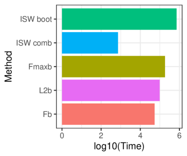
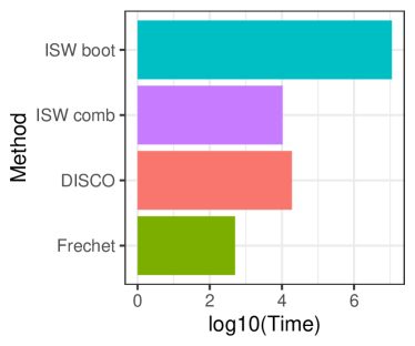
Figure 2: Running times for (a) real line and (b) circle experiments.
Refer to caption Refer to caption Refer to caption Refer to caption
(a) (b) (c) (d)
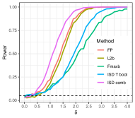
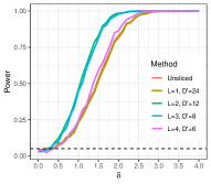
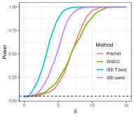
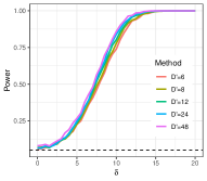
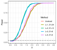
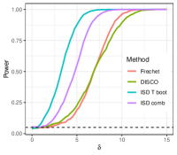
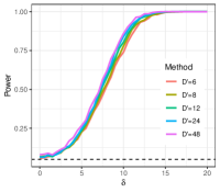
Figure 3: Performances on synthetic data. Dotted lines indicates nominal size of all tests (α=0.05𝛼0.05\alpha=0.05). (a) comparison with existing methods on finite interval—a test based on basis function representation (Gorecki & Smaga, 2015, FP), a sum-type 2subscript2\ell_{2} norm-based test (L2b) (Zhang, 2013), and a max-type test (Zhang et al., 2019) that uses the maximum of coordinate-wise F𝐹F statistic (Fmaxb), (b) unsliced vs. different settings of (L,D)𝐿superscript𝐷(L,D^{\prime}) on finite interval. (c) Circular data, comparing with Fréchet ANOVA (Dubey & Müller, 2019), and the DISCO nonparametric test (Rizzo & Székely, 2010); (d) harmonic combination tests on cylindrical data for L=4𝐿4L=4. .

6 Experiments

We compare the performance of our tests with several existing methods, across synthetic and real data, and settings of the embedding parameters L,D𝐿superscript𝐷L,D^{\prime}. For evaluation, we use empirical power at different degrees of departure from the null hypothesis (Captured by δ𝛿\delta in the plots in Fig. 3), calculated by averaging the proportion of rejections at level α=0.05𝛼0.05\alpha=0.05 over 1000 independent datasets, with samples divided into two groups of sizes n1=60,n2=40formulae-sequencesubscript𝑛160subscript𝑛240n_{1}=60,n_{2}=40. To ensure the tests are well-calibrated, we calculate nominal sizes assuming the two sample groups are drawn from the same meta-distribution. Details on the experiment settings and computational complexity are in Appendix B.1.

Finite intervals

We use embedding dimensions L=3,D=10formulae-sequence𝐿3superscript𝐷10L=3,D^{\prime}=10 to compare our method against 11 functional ANOVA tests—we report results for 3 of them in Figure 3a (see Appendix B for complete results). All methods maintain nominal size for δ=0𝛿0\delta=0 (Figure 3a). While the combination test (ISD comb) based on our proposal outperformed all the other tests across all values of δ𝛿\delta, the bootstrap test that uses the overall 𝕋𝕋\mathbb{T} statistic (ISD T boot) performs better than Fmaxb but worse than others. In terms of computation time, ISD comb takes the least amount of time (Fig. 2a).

We also compare the p𝑝p-value combination test based on an unsliced 24-dimensional inverse CDF embedding with sliced IS𝒲2𝐼𝑆subscript𝒲2IS\mathcal{W}_{2}-based tests (Figure 3b). We use multiple pairs of (L,D)𝐿superscript𝐷(L,D^{\prime}) values, all of them giving overall embeddings of dimension D=LD=24𝐷𝐿superscript𝐷24D=LD^{\prime}=24. The performance of an IS𝒲2𝐼𝑆subscript𝒲2IS\mathcal{W}_{2}-based test that uses slicing over only the first eigenfunction is almost as good as the unsliced version. With more eigenfunctions, the powers first improve considerably, then become similar to the unsliced version again.

Manifold domains

We consider data from distributions on circles and cylinders. For circular data, we take von Mises distributions with randomly chosen parameters as our samples. For an angle x𝑥x (measured in radians), the von Mises probability density function is given by f(x|μ,κ)=exp[κcos(xμ)](2πI0(κ))1𝑓conditional𝑥𝜇𝜅𝜅𝑥𝜇superscript2𝜋subscript𝐼0𝜅1f(x|\mu,\kappa)=\exp[\kappa\cos(x-\mu)](2\pi I_{0}(\kappa))^{-1}, where I0(κ)subscript𝐼0𝜅I_{0}(\kappa) is the modified Bessel function of order 0. We fix κ=2𝜅2\kappa=2, and use μμiN(0,0.12)𝜇subscript𝜇𝑖similar-to𝑁0superscript0.12\mu\equiv\mu_{i}\sim N(0,0.1^{2}), μνiN(δ,0.12)𝜇subscript𝜈𝑖similar-to𝑁𝛿superscript0.12\mu\equiv\nu_{i}\sim N(\delta,0.1^{2}) for samples from group 1 and 2 respectively—with δ[0,15]×π/180𝛿015𝜋180\delta\in[0,15]\times\pi/180 (i.e. 0 to 15 degrees converted to radians). As each observation vector, we take 100 random draws from each sample-specific distribution. For our embeddings, we use L=10,D=20formulae-sequence𝐿10superscript𝐷20L=10,D^{\prime}=20. Since the competing methods cannot handle circular geometry directly, to implement them we cut the circle into an interval. Figure 3c shows that all methods maintain nominal size, but both our tests maintain considerably higher power than existing methods for all δ𝛿\delta. Computationally, ISD comb has comparable order of magnitude as the other two methods (Fig. 2b).

To generate cylindrical data, we use the distribution proposed by Mardia & Sutton (1978). Samples from each distribution have the form of a bivariate random vector (Θ,X)Θ𝑋(\Theta,X), where the first (circular) marginal ΘΘ\Theta has a von Mises distribution, and X𝑋X is a Gaussian conditional on Θ=θΘ𝜃\Theta=\theta. We draw the mean parameters for each coordinate-wise distribution from Unif(0,1)Unif01\text{{Unif}}(0,1) and Unif(δ,δ+1)Unif𝛿𝛿1\text{{Unif}}(\delta,\delta+1) for sample groups 1 and 2 respectively, with δ[0,30]×π/180𝛿030𝜋180\delta\in[0,30]\times\pi/180. We then use 500 random draws from each sample distribution to obtain histograms. To evaluate the effects of choosing L,D𝐿superscript𝐷L,D^{\prime} we calculate our embeddings for L{2,3,4,5},D{6,8,12,24,48}formulae-sequence𝐿2345superscript𝐷68122448L\in\{2,3,4,5\},D^{\prime}\in\{6,8,12,24,48\}. The choice of L𝐿L has small effect on performance, so we report results for L=4𝐿4L=4 in Figure 3d. Higher values of Dsuperscript𝐷D^{\prime} result in some increase in power.

Comparison to existing slicing methods

As an example showcasing the importance of using intrinsic distances, consider the following graph setup: points A and B are adjacent on a planar regular 200-gon, with the edge AB removed. The intrinsic distance between A and B is large and the (extrinsic) Euclidean distance is small. No matter what Euclidean projection we use, the SW cost of moving probability mass from A to B would be small, leading to testing power loss when we compare two distribution sets that concentrate one around A and the other around B. To numerically analyze this case we generate distributions on this graph by putting Unif(0,1) weights at each of the vertices, and added an additional weight of 10 to the bin at point A to obtain the first set of distributions with a mode at A. For the second set we put the weight of 10 at B instead to obtain a set of distributions with mode at B.

Method Power Size Time (sec)
IS𝒲2𝐼𝑆subscript𝒲2IS\mathcal{W}_{2} 1.00 0.029 630.67
SW 0.128 0.029 579.3
GSW-circle 0.128 0.029 564.82
GSW-poly3 0.025 0.025 779.69
GSW-poly5 0.044 0.035 1009.85
MSW 1.00 0.63 61764.22
ST 1.00 0.048 21474.88
Table 1: Comparison of multiple slicing techniques.

Table 1 shows comparison of IS𝒲2𝐼𝑆subscript𝒲2IS\mathcal{W}_{2} with Sliced Wasserstein (SW) in two dimensions, GSW with 3 choices of defining functions (circular, homogeneous polynomial of degree 3, and degree 5), MSW, and Sobolev transport (ST). We use L=10,D=8formulae-sequence𝐿10superscript𝐷8L=10,D^{\prime}=8 to produce all embeddings, and implement the sliced version of ST by aggregating ST distances originating from 10 random vertices. IS𝒲2𝐼𝑆subscript𝒲2IS\mathcal{W}_{2} achieves the highest possible power, maintains nominal type-I error, and has computational time comparable to SW/GSW. ST and MSW achieve the same power as IS𝒲2𝐼𝑆subscript𝒲2IS\mathcal{W}_{2}, but take much longer. This is because unlike slicing-based methods, they need to rely on permutation testing in absence of embeddings. For MSW, the high power comes at the price of a size that is much higher than the acceptable threshold of 0.05.

Age Groups 6–15 16–25 26–35 36–45 46–55 56–65 66–75 76–85
6–15 0.394 0.098 0.555 0.882 0.985 0.919 0.997
16–25 1.2e-13 0.575 0.967 0.126 0.921 0.911 0.977
26–35 3.1e-21 2.7e-04 0.459 0.197 0.996 0.919 0.565
36–45 6.1e-22 7.9e-08 0.042 0.864 0.637 0.849 0.991
46–55 8.2e-22 4.7e-05 0.011 0.343 0.841 0.165 0.554
56–65 1.3e-25 0.001 0.001 5.6e-05 0.003 0.991 0.962
66–75 3.6e-35 7.8e-12 1.5e-11 4.6e-15 1.8e-13 0.001 0.989
76–85 3.8e-46 1.4e-26 1.7e-30 8.4e-37 2.1e-35 1.3e-17 6.5e-09
Table 2: Activity intensity comparison across age groups in the NHANES data. Below diagonal: p𝑝p-values for the actual data comparisons. Above diagonal: null p𝑝p-values obtained by combining and randomly splitting the two groups. Bold entries correspond to rejected hypotheses with the BH procedure at FDR level 0.1.
Crime Type Tue vs Thu Tue vs Sat
Theft 0.428 4.2e-06
Deceptive Pract. 0.313 0.001
Battery 0.430 0.001
Robbery 0.119 0.003
Narcotics 0.854 0.004
Criminal Dam. 0.855 0.02
Other Offense 0.931 0.052
Burglary 0.142 0.261
Assault 0.997 0.38
Motor Veh. Theft 0.858 0.416
Table 3: Chicago Crime analysis p𝑝p-values. Bold entries correspond to rejected hypotheses with the BH procedure at FDR level 0.1.

7 Real Data Examples

NHANES

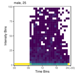
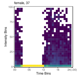
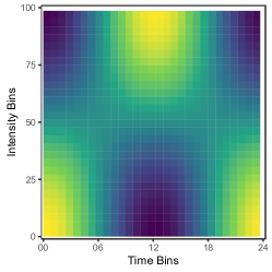
This dataset (NHANES, 2008) contains physical activity pattern readings for 6839 individuals, corresponding to activity monitor intensity values for 24×60=14402460144024\times 60=1440 minutes throughout the day, over 7 days. We capture this activity pattern into a cylindrical histogram with time and intensity dimensions, having 96 and 100 bins respectively. Since the time dimension is periodic, normalized counts of this histogram can be considered as person-specific probability distributions over the cylinder S1(T1)×[0,T2)superscript𝑆1subscript𝑇10subscript𝑇2S^{1}(T_{1})\times[0,T_{2}), with T1=96,T2=100formulae-sequencesubscript𝑇196subscript𝑇2100T_{1}=96,T_{2}=100. To check if activity patterns vary across different groups of individuals, we first split individuals into age-specific groups: 6–15, 16–25, …,76–85, then sample 100 males and 100 females from each split. For our analysis, we consider L=3𝐿3L=3 indices along the two directions, i.e. 1,2=1,2,3formulae-sequencesubscript1subscript2123\ell_{1},\ell_{2}=1,2,3 and D=5superscript𝐷5D^{\prime}=5. We summarize the p𝑝p-value combination test results in Table 6, below the diagonal. We control false discovery rate at 0.10.10.1 by running the resulting p𝑝p-values through the procedure of Benjamini & Hochberg (1995). IS𝒲2𝐼𝑆subscript𝒲2IS\mathcal{W}_{2} detects statistically significant differences between all pairs of groups, except the 36–45 and 46–55 groups. As expected, the control p𝑝p-values—obtained by mixing male and female samples in each age group and splitting arbitrarily—do not concentrate near zero. More details are given in Appendix B.2.

Chicago Crime

We use this dataset (City of Chicago, 2022) to show a practical usage of our method on histograms over graphs. Each beat (geographic area subdivision used by police) corresponds to a vertex, and two vertices are connected by an edge if the corresponding beats share a geographic boundary. For each crime type and day, the normalized counts of that crime type for each beat gives a daily probability distribution over the graph. Our goal is to compare the collection of distributions of, say, theft occurring on Tuesday to those of Thursday and Saturday. The Tuesday versus Thursday comparison is intended as a null case, as we do not expect to see any differences between them (Rustamov & Klosowski, 2020). Table 7 results IS𝒲2𝐼𝑆subscript𝒲2IS\mathcal{W}_{2} outcomes using 100-dimensional embeddings (L=20,D=5formulae-sequence𝐿20superscript𝐷5L=20,D^{\prime}=5).We detect statistically significant differences between Tuesday and Saturday patterns for six categories of crime, and as expected, no differences between Tuesday and Thursday patterns. For more details and another graph-based application, see Appendices B.3 and B.4, respectively.

8 Conclusion

In this paper we have introduced a novel class of sliced Wasserstein distances on manifolds and graphs, and applied the resulting IS𝒲2𝐼𝑆subscript𝒲2IS\mathcal{W}_{2} distance in the context of hypothesis tests for meta-distributions on general domains, due to the high relevance of this setup in real data situations. It is worth pointing out that the assumption-lean nature of IS𝒲2𝐼𝑆subscript𝒲2IS\mathcal{W}_{2} can enable its adoption by many other statistical and ML methods.

The IS𝒲2𝐼𝑆subscript𝒲2IS\mathcal{W}_{2} embeddings can be used to do other hypothesis tests, such as tests for equality of covariances by extending the notion of Wasserstein covariances from (Petersen & Müller, 2019) to general domains. The embeddings can also be used as input features for supervised learning problems over distributions. In another direction, IS𝒲2𝐼𝑆subscript𝒲2IS\mathcal{W}_{2} is directly applicable as a loss function for generative modeling. For example, if one is generating distributions over a graph or manifold, IS𝒲2𝐼𝑆subscript𝒲2IS\mathcal{W}_{2} can serve as a loss function similarly to how other sliced distances are used in this context over Euclidean domains.

The proposed framework has a few limitations. There is scope of exploration for choosing the parameters L𝐿L and Dsuperscript𝐷D^{\prime} in a principled manner. Empirical computation of eigenfunctions for general manifolds will introduce approximation errors that need to be tackled by expanding our theoretical results. In terms of potential societal impacts of our proposal, any difference between data distributions from different demographic groups found using our method should be evaluated in light of potential biases in the data collection stage.

References

  • Aine et al. (2017) Aine, C. J., Bockholt, H. J., Bustillo, J. R., et al. Multimodal neuroimaging in schizophrenia: Description and dissemination. Neuroinformatics, 15(4):343–364, Oct 2017. ISSN 1559-0089.
  • Arroyo Relión et al. (2019) Arroyo Relión, J. D., Kessler, D., Levina, E., and Taylor, S. F. Network classification with applications to brain connectomics. Ann. Appl. Stat., 13(3):1648–1677, 09 2019.
  • Bakhvalov (2015) Bakhvalov, N. S. On the approximate calculation of multiple integrals. J. Complexity, 31:502–516, 2015. English translation; the original appeared in Vestnik MGU, Ser. Math. Mech. Astron. Phys. Chem, 4, 3–18, 1959.
  • Benjamini & Hochberg (1995) Benjamini, Y. and Hochberg, Y. Controlling the false discovery rate: A practical and powerful approach to multiple testing. Journal of the Royal Statistical Society. Series B (Methodological), 57(1):289–300, 1995. ISSN 00359246.
  • Berger (2003) Berger, M. A Panoramic View of Riemannian Geometry. Springer-Verlag Berlin Heidelberg, 2003.
  • Bigot (2020) Bigot, J. Statistical data analysis in the wasserstein space. ESAIM: ProcS, 68:1–19, 2020.
  • Borden & Luscombe (2017) Borden, B. and Luscombe, J. Essential Mathematics for the Physical Sciences, volume Volume I: Homogeneous boundary value problems, Fourier methods, and special functions, chapter Spherical harmonics and friends. Morgan & Claypool Publishers, 2017. Pages 6–1 to 6–26.
  • Brown & Steinerberger (2020) Brown, L. and Steinerberger, S. On the Wasserstein distance between classical sequences and the Lebesgue measure. Trans. Amer. Math. Soc., in press, 2020. https://arxiv.org/abs/1909.09046.
  • City of Chicago (2022) City of Chicago. Chicago data portal: Crimes - 2018, 2022. URL https://data.cityofchicago.org/Public-Safety/Crimes-2018/3i3m-jwuy.
  • Coifman & Lafon (2006) Coifman, R. R. and Lafon, S. Diffusion maps. Applied and Computational Harmonic Analysis, 21(1):5 – 30, 2006. ISSN 1063-5203. Special Issue: Diffusion Maps and Wavelets.
  • Dehling & Fried (2012) Dehling, H. and Fried, R. Asymptotic distribution of two-sample empirical U-quantiles with applications to robust tests for shifts in location. Journal of Multivariate Analysis, 105(1):124–140, 2012.
  • Deshpande et al. (2019) Deshpande, I., Hu, Y.-T., Sun, R., Pyrros, A., Siddiqui, N., Koyejo, S., Zhao, Z., Forsyth, D., and Schwing, A. G. Max-sliced wasserstein distance and its use for gans. In 2019 IEEE/CVF Conference on Computer Vision and Pattern Recognition (CVPR), pp.  10640–10648, 2019.
  • Dubey & Müller (2019) Dubey, P. and Müller, H.-G. Frćhet analysis of variance for random objects. Biometrika, 106(4):803–821, 10 2019. ISSN 0006-3444.
  • Gavish et al. (2019) Gavish, N., Nyquist, P., and Peletier, M. Large deviations and gradient flows for the Brownian one-dimensional hard-rod system. https://arxiv.org/abs/1909.02054, 2019.
  • Good (1958) Good, I. J. Significance tests in parallel and in series. Journal of the American Statistical Association, 53(284):799–813, 1958. ISSN 01621459.
  • Gorecki & Smaga (2015) Gorecki, T. and Smaga, L. A Comparison of Tests for the One-Way ANOVA Problem for Functional Data. Computational Statistics, 30:987–1010, 2015.
  • Gretton et al. (2012) Gretton, A., Borgwardt, K. M., Rasch, M. J., Schölkopf, B., and Smola, A. A kernel two-sample test. J. Mach. Learn. Res., 13:723–773, March 2012. ISSN 1532-4435.
  • Hu et al. (2015) Hu, J., Shi, Y., and Xu, B. The gradient estimate of a neumann eigenfunction on a compact manifold with boundary. Chinese Annals of Mathematics, Series B, 36(6):991–1000, Nov 2015. ISSN 1860-6261.
  • Huang et al. (2006) Huang, Y., Xu, H., Calian, V., and Hsu, J. C. To permute or not to permute. Bioinformatics, 22(18):2244–2248, 07 2006. ISSN 1367-4803.
  • Kolouri et al. (2019a) Kolouri, S., Nadjahi, K., Simsekli, U., Badeau, R., and Rohde, G. Generalized sliced wasserstein distances. In Wallach, H., Larochelle, H., Beygelzimer, A., Alché-Buc, F., Fox, E., and Garnett, R. (eds.), Advances in Neural Information Processing Systems 32, pp.  261–272. Curran Associates, Inc., 2019a.
  • Kolouri et al. (2019b) Kolouri, S., Pope, P. E., Martin, C. E., and Rohde, G. K. Sliced wasserstein auto-encoders. In 7th International Conference on Learning Representations, ICLR 2019, New Orleans, LA, USA, May 6-9, 2019. OpenReview.net, 2019b. URL https://openreview.net/forum?id=H1xaJn05FQ.
  • Lai & Zhao (2017) Lai, R. and Zhao, H. Multiscale Nonrigid Point Cloud Registration Using Rotation-Invariant Sliced-Wasserstein Distance via Laplace–Beltrami Eigenmap. In SIAM J. Imaging Sci., volume 10 of 2, pp. 449–483, 2017.
  • Le et al. (2019) Le, T., Yamada, M., Fukumizu, K., and Cuturi, M. Tree-sliced variants of wasserstein distances. In Advances in Neural Information Processing Systems, volume 32, 2019.
  • Le et al. (2022) Le, T., Nguyen, T., Phung, D., and Anh Nguyen, V. Sobolev transport: A scalable metric for probability measures with graph metrics. In Proceedings of The 25th International Conference on Artificial Intelligence and Statistics, volume 151 of Proceedings of Machine Learning Research, pp.  9844–9868. PMLR, 2022.
  • Lipman et al. (2010) Lipman, Y., Rustamov, R. M., and Funkhouser, T. A. Biharmonic distance. ACM Trans. Graph., 29(3), July 2010. ISSN 0730-0301.
  • Liu & Xie (2020) Liu, Y. and Xie, J. Cauchy combination test: A powerful test with analytic p-value calculation under arbitrary dependency structures. Journal of the American Statistical Association, 115(529):393–402, 2020.
  • Mardia & Sutton (1978) Mardia, K. V. and Sutton, T. W. A Model for Cylindrical Variables with Applications. Journal of the Royal Statistical Society: Series B (Methodological), 40(2):229–233, 1978.
  • Micchelli et al. (2006) Micchelli, C. A., Xu, Y., and Zhang, H. Universal kernels. J. Mach. Learn. Res., 7:2651–2667, December 2006. ISSN 1532-4435.
  • Murray & Rice (1993) Murray, M. K. and Rice, J. W. Differential Geometry and Statistics, chapter The definition of a statistical manifold (Chapter 3.2). Chapman & Hall, 1993.
  • NHANES (2008) NHANES. 2005-2006 Data Documentation, Codebook, and Frequencies, 2008. URL {https://wwwn.cdc.gov/Nchs/Nhanes/2005-2006/PAXRAW_D.htm}.
  • Panaretos & Zemel (2019) Panaretos, V. M. and Zemel, Y. Statistical aspects of wasserstein distances. Annual Review of Statistics and Its Application, 6(1):405–431, 2019.
  • Petersen & Müller (2016) Petersen, A. and Müller, H.-G. Functional data analysis for density functions by transformation to a hilbert space. Ann. Statist., 44(1):183–218, 02 2016.
  • Petersen & Müller (2019) Petersen, A. and Müller, H.-G. Wasserstein covariance for multiple random densities. Biometrika, 106(2):339–351, 04 2019. ISSN 0006-3444. doi: 10.1093/biomet/asz005. URL https://doi.org/10.1093/biomet/asz005.
  • Peyré & Cuturi (2019) Peyré, G. and Cuturi, M. Computational optimal transport: With applications to data science. Foundations and Trends in Machine Learning, 11(5-6):355–607, 2019. ISSN 1935-8237.
  • Power et al. (2011) Power, J. D., Cohen, A. L., Nelson, S. M., et al. Functional network organization of the human brain. Neuron, 72(4):665–678, Nov 2011. ISSN 1097-4199. 22099467[pmid].
  • Reed & Simon (1080) Reed, M. and Simon, B. Methods of modern mathematical physics. Vol. 1: Functional Analysis. Academic Press, 1080.
  • Reuter et al. (2009) Reuter, M., Wolter, F.-E., Shenton, M., and Niethammer, M. Laplace-Beltrami eigenvalues and topological features of eigenfunctions for statistical shape analysis. Computer-Aided Design, 41(10):739–755, 2009.
  • Rizzo & Székely (2010) Rizzo, M. L. and Székely, G. J. DISCO analysis: A nonparametric extension of analysis of variance. Ann. Appl. Stat., 4:1034–1055, 2010.
  • Rubner et al. (2000) Rubner, Y., Tomasi, C., and Guibas, L. J. The earth mover’s distance as a metric for image retrieval. International Journal of Computer Vision, 40(2):99–121, 2000. doi: 10.1023/A:1026543900054.
  • Rustamov & Klosowski (2020) Rustamov, R. M. and Klosowski, J. T. Kernel mean embedding based hypothesis tests for comparing spatial point patterns. Spatial Statistics, 38:100459, 2020. ISSN 2211-6753.
  • Serfling (2009) Serfling, R. J. Approximation theorems of mathematical statistics. John Wiley & Sons, 2009.
  • Solomon et al. (2014) Solomon, J., Rustamov, R. M., Guibas, L. J., and Butscher, A. Wasserstein propagation for semi-supervised learning. In Proceedings of the 31th International Conference on Machine Learning, ICML 2014, Beijing, China, 21-26 June 2014, volume 32 of JMLR Workshop and Conference Proceedings, pp.  306–314. JMLR.org, 2014.
  • Villani (2003) Villani, C. Topics in optimal transportation. Graduate studies in mathematics. American mathematical society, Providence, Rhode Island, 2003. ISBN 0-8218-3312-X.
  • Wilson (2019) Wilson, D. J. The harmonic mean p-value for combining dependent tests. Proceedings of the National Academy of Sciences, 116(4):1195–1200, 2019. ISSN 0027-8424.
  • Zhang (2013) Zhang, J.-T. Analysis of Variance for Functional Data. Chapman and Hall/CRC, first edition, 2013.
  • Zhang et al. (2019) Zhang, J.-T., Chen, M.-Y., Wu, H.-T., and Zhou, B. A new test for functional one-way ANOVA with applications to ischemic heart screening. Computational Statistics & Data Analysis, 132:3–17, 2019.

Appendix

For the appendix to be self-contained, we restate results (theory and experiments) in the main paper when necessary. Appendix A contains proofs of theoretical results and some implementation details. Details and results of experiments performed are in Appendix B. Code and data behind these experiments are at https://github.com/shubhobm/isw.

Appendix A Proofs and additional results

A.1 Proofs and Notes for Section 3

Proposition 3.4.

For P,Q𝒫(𝒫(𝒳))𝑃𝑄𝒫𝒫𝒳P,Q\in\mathcal{P}(\mathcal{P}(\mathcal{X})), the following equality holds:

𝕋(P,Q)=𝔼μP,νQ[𝒟2(μ,ν)]12𝔼μ,μP[𝒟2(μ,μ)]12𝔼ν,νQ[𝒟2(ν,ν)],𝕋𝑃𝑄subscript𝔼formulae-sequencesimilar-to𝜇𝑃similar-to𝜈𝑄delimited-[]superscript𝒟2𝜇𝜈12subscript𝔼similar-to𝜇superscript𝜇𝑃delimited-[]superscript𝒟2𝜇superscript𝜇12subscript𝔼similar-to𝜈superscript𝜈𝑄delimited-[]superscript𝒟2𝜈superscript𝜈\mathbb{T}({P},{Q})=\mathbb{E}_{\mu\sim{P},\nu\sim{Q}}[\mathcal{D}^{2}(\mu,\nu)]-\frac{1}{2}\mathbb{E}_{\mu,\mu^{\prime}\sim{P}}[\mathcal{D}^{2}(\mu,\mu^{\prime})]-\frac{1}{2}\mathbb{E}_{\nu,\nu^{\prime}\sim{Q}}[\mathcal{D}^{2}(\nu,\nu^{\prime})], (5)

where to avoid notational clutter we use 𝒟2(,)superscript𝒟2\mathcal{D}^{2}(\cdot,\cdot) as a shorthand for (𝒟(,))2superscript𝒟2(\mathcal{D}(\cdot,\cdot))^{2}.

Proof.

This is a straightforward application of the “kernel trick”: using the Hilbert property of the distance we can rewrite,

𝔼μP,νQsubscript𝔼formulae-sequencesimilar-to𝜇𝑃similar-to𝜈𝑄\displaystyle\mathbb{E}_{\mu\sim{P},\nu\sim{Q}} [η(μ)η(ν)2]12𝔼μ,μP[η(μ)η(μ)2]12𝔼ν,νQ[η(ν)η(ν)2]delimited-[]superscriptsubscriptnorm𝜂𝜇𝜂𝜈212subscript𝔼similar-to𝜇superscript𝜇𝑃delimited-[]superscriptsubscriptnorm𝜂𝜇𝜂superscript𝜇212subscript𝔼similar-to𝜈superscript𝜈𝑄delimited-[]superscriptsubscriptnorm𝜂𝜈𝜂superscript𝜈2\displaystyle[\|\eta(\mu)-\eta(\nu)\|_{\mathcal{\mathcal{H}}}^{2}]-\frac{1}{2}\mathbb{E}_{\mu,\mu^{\prime}\sim{P}}[\|\eta(\mu)-\eta(\mu^{\prime})\|_{\mathcal{\mathcal{H}}}^{2}]-\frac{1}{2}\mathbb{E}_{\nu,\nu^{\prime}\sim{Q}}[\|\eta(\nu)-\eta(\nu^{\prime})\|_{\mathcal{\mathcal{H}}}^{2}]
=\displaystyle= 𝔼μP[η(μ)2]+𝔼νQ[η(ν)2]2𝔼μP[η(μ)],𝔼νQ[η(ν)]subscript𝔼similar-to𝜇𝑃delimited-[]superscriptsubscriptnorm𝜂𝜇2subscript𝔼similar-to𝜈𝑄delimited-[]superscriptsubscriptnorm𝜂𝜈22subscriptsubscript𝔼similar-to𝜇𝑃delimited-[]𝜂𝜇subscript𝔼similar-to𝜈𝑄delimited-[]𝜂𝜈\displaystyle\mathbb{E}_{\mu\sim{P}}[\|\eta(\mu)\|_{\mathcal{H}}^{2}]+\mathbb{E}_{\nu\sim{Q}}[\|\eta(\nu)\|_{\mathcal{\mathcal{H}}}^{2}]-2\langle\mathbb{E}_{\mu\sim{P}}[\eta(\mu)],\mathbb{E}_{\nu\sim{Q}}[\eta(\nu)]\rangle_{\mathcal{H}}
\displaystyle- 𝔼μP[η(μ)2]𝔼νQ[η(ν)2]subscript𝔼similar-to𝜇𝑃delimited-[]superscriptsubscriptnorm𝜂𝜇2subscript𝔼similar-to𝜈𝑄delimited-[]superscriptsubscriptnorm𝜂𝜈2\displaystyle\mathbb{E}_{\mu\sim{P}}[\|\eta(\mu)\|_{\mathcal{H}}^{2}]-\mathbb{E}_{\nu\sim{Q}}[\|\eta(\nu)\|_{\mathcal{\mathcal{H}}}^{2}]
+\displaystyle+ 𝔼μP[η(μ)],𝔼μP[η(μ)]+𝔼νQ[η(ν)],𝔼νQ[η(ν)]subscriptsubscript𝔼similar-to𝜇𝑃delimited-[]𝜂𝜇subscript𝔼similar-to𝜇𝑃delimited-[]𝜂𝜇subscriptsubscript𝔼similar-to𝜈𝑄delimited-[]𝜂𝜈subscript𝔼similar-to𝜈𝑄delimited-[]𝜂𝜈\displaystyle\langle\mathbb{E}_{\mu\sim{P}}[\eta(\mu)],\mathbb{E}_{\mu\sim{P}}[\eta(\mu)]\rangle_{\mathcal{H}}+\langle\mathbb{E}_{\nu\sim{Q}}[\eta(\nu)],\mathbb{E}_{\nu\sim{Q}}[\eta(\nu)]\rangle_{\mathcal{H}}
=\displaystyle= 𝔼μP[η(μ)]𝔼νQ[η(ν)]2=𝕋(P,Q).superscriptsubscriptnormsubscript𝔼similar-to𝜇𝑃delimited-[]𝜂𝜇subscript𝔼similar-to𝜈𝑄delimited-[]𝜂𝜈2𝕋𝑃𝑄\displaystyle\|\mathbb{E}_{\mu\sim{P}}[\eta(\mu)]-\mathbb{E}_{\nu\sim{Q}}[\eta(\nu)]\|_{\mathcal{H}}^{2}=\mathbb{T}({P},{Q}).

Which gives the sought equivalence. ∎

A.2 Proofs and Notes for Section 4.1

Proposition 4.2.

If 𝒳𝒳\mathcal{X} is a smooth compact n𝑛n-dimensional manifold and λ(n1)/2α(λ)<subscriptsuperscriptsubscript𝜆𝑛12𝛼subscript𝜆\sum_{\ell}\lambda_{\ell}^{(n-1)/2}\alpha(\lambda_{\ell})<\infty, then IS𝒲2𝐼𝑆subscript𝒲2IS\mathcal{W}_{2} is well-defined.

Proof.

We use Hörmander’s bound on the supremum norm of the eigenfunctions:

ϕcλ(n1)/4ϕ2,subscriptnormsubscriptitalic-ϕ𝑐superscriptsubscript𝜆𝑛14subscriptnormsubscriptitalic-ϕ2\|\phi_{\ell}\|_{\infty}\leq c\lambda_{\ell}^{(n-1)/4}\|\phi_{\ell}\|_{2},

for some constant c𝑐c that depends on the manifold. By orthonormality of the eigenfunctions we have ,ϕ2=1for-allsubscriptnormsubscriptitalic-ϕ21\forall\ell,\|\phi_{\ell}\|_{2}=1. Next, note that 𝒲2(ϕμ,ϕν)2ϕsubscript𝒲2subscriptitalic-ϕ𝜇subscriptitalic-ϕ𝜈2subscriptnormsubscriptitalic-ϕ\mathcal{W}_{2}(\phi_{\ell}\sharp\mu,\phi_{\ell}\sharp\nu)\leq 2\|\phi_{\ell}\|_{\infty} as the maximum distance that the mass would be transported in any transportation plan involving pushforwards via ϕsubscriptitalic-ϕ\phi_{\ell} is upper bounded by 2ϕ2subscriptnormsubscriptitalic-ϕ2\|\phi_{\ell}\|_{\infty}. As a result, every term in the series defining IS𝒲2𝐼𝑆subscript𝒲2IS\mathcal{W}_{2} can be upper-bounded by the terms of the following series:

4ϕ2α(λ)4c2λ(n1)/2α(λ)λ(n1)/2α(λ),subscript4superscriptsubscriptnormsubscriptitalic-ϕ2𝛼subscript𝜆subscript4superscript𝑐2superscriptsubscript𝜆𝑛12𝛼subscript𝜆proportional-tosubscriptsuperscriptsubscript𝜆𝑛12𝛼subscript𝜆\sum_{\ell}4\|\phi_{\ell}\|_{\infty}^{2}\alpha(\lambda_{\ell})\leq\sum_{\ell}4c^{2}\lambda_{\ell}^{(n-1)/2}\alpha(\lambda_{\ell})\propto\sum_{\ell}\lambda_{\ell}^{(n-1)/2}\alpha(\lambda_{\ell}),

which proves the claim by the direct comparison test for convergence of series. ∎

Remark A.1.

When Weyl law applies, we have that λ=Θ(2/n)subscript𝜆Θsuperscript2𝑛\lambda_{\ell}=\Theta(\ell^{2/n}), which allows us to replace the above condition by (n1)/nα(λ)<subscriptsuperscript𝑛1𝑛𝛼subscript𝜆\sum_{\ell}\ell^{(n-1)/n}\alpha(\lambda_{\ell})<\infty. For the diffusion kernel/distance choice of α(λ)=etλ𝛼𝜆superscript𝑒𝑡𝜆\alpha(\lambda)=e^{-t\lambda} the series always converges independently of the manifold dimension. For biharmonic choice of α(λ)=1/λ2𝛼𝜆1superscript𝜆2\alpha(\lambda)=1/\lambda^{2}, the sufficient condition is the convergence of (n1)/n/λ2(n1)/n/(2/n)2=(n5)/nsimilar-tosubscriptsuperscript𝑛1𝑛superscriptsubscript𝜆2subscriptsuperscript𝑛1𝑛superscriptsuperscript2𝑛2subscriptsuperscript𝑛5𝑛\sum_{\ell}\ell^{(n-1)/n}/\lambda_{\ell}^{2}\sim\sum_{\ell}\ell^{(n-1)/n}/(\ell^{2/n})^{2}=\sum_{\ell}\ell^{(n-5)/n}, where we applied Weyl’s asymptotic again. As a result, the biharmonic choice of α𝛼\alpha is guaranteed to provide a well-defined IS𝒲2𝐼𝑆subscript𝒲2IS\mathcal{W}_{2} for 1 and 2-dimensional manifolds. Notice, however, that the Hörmander’s bound used in the proof of the above proposition can be rather lax in some of the settings that are practically relevant, such as the product spaces of lines and circles (where all of the eigenfunctions are bounded by a constant as can be seen from Table 4), and, thus, convergence for the biharmonic choice holds more widely.

Proposition 4.3.

If 𝒟𝒟\mathcal{D} is a Hilbertian probability distance such that IS𝒟𝐼𝑆𝒟IS\mathcal{D} is well-defined, then

(i) IS𝒟𝐼𝑆𝒟IS\mathcal{D} is Hilbertian, and

(ii) IS𝒟𝐼𝑆𝒟IS\mathcal{D} satisfies the following metric properties: non-negativity, symmetry, the triangle inequality, and IS𝒟(μ,μ)=0𝐼𝑆𝒟𝜇𝜇0IS\mathcal{D}(\mu,\mu)=0.

Proof.

By Hilbertian property of 𝒟𝒟\mathcal{D}, there exists a Hilbert space 0superscript0\mathcal{H}^{0} and a map η0:𝒫()0:superscript𝜂0𝒫superscript0\eta^{0}:\mathcal{P}(\mathbb{R})\rightarrow\mathcal{H}^{0} such that 𝒟(ρ1,ρ2)=η0(ρ1)η0(ρ2)0𝒟subscript𝜌1subscript𝜌2subscriptnormsuperscript𝜂0subscript𝜌1superscript𝜂0subscript𝜌2superscript0\mathcal{D}(\rho_{1},\rho_{2})=\|\eta^{0}(\rho_{1})-\eta^{0}(\rho_{2})\|_{\mathcal{H}^{0}} for all ρ1,ρ2𝒫()subscript𝜌1subscript𝜌2𝒫\rho_{1},\rho_{2}\in\mathcal{P}(\mathbb{R}). Plugging this into the definition of IS𝒟𝐼𝑆𝒟IS\mathcal{D} we have IS𝒟(μ,ν)=η(μ)η(ν)𝐼𝑆𝒟𝜇𝜈subscriptnorm𝜂𝜇𝜂𝜈IS\mathcal{D}(\mu,\nu)=\|\eta(\mu)-\eta(\nu)\|_{\mathcal{\mathcal{H}}}, where =0subscriptdirect-sumsuperscript0\mathcal{H}=\oplus_{\ell}\mathcal{H}^{0} and the \ell-th component of η(μ)𝜂𝜇\eta(\mu) is α(λ)η0(ϕμ)0𝛼subscript𝜆subscript𝜂0subscriptitalic-ϕ𝜇superscript0\sqrt{\alpha(\lambda_{\ell})}\eta_{0}(\phi_{\ell}\sharp\mu)\in\mathcal{H}^{0}. The second part of Proposition Proposition 4.3 directly follows from the Hilbert property. ∎

Proposition A.1.

When μ=δx(),ν=δy()formulae-sequence𝜇subscript𝛿𝑥𝜈subscript𝛿𝑦\mu=\delta_{x}(\cdot),\nu=\delta_{y}(\cdot) for two points x,y𝒳𝑥𝑦𝒳x,y\in\mathcal{X}, we have IS𝒲2(μ,ν)=d(x,y)𝐼𝑆subscript𝒲2𝜇𝜈𝑑𝑥𝑦IS\mathcal{W}_{2}(\mu,\nu)=d(x,y), where d(,)𝑑d(\cdot,\cdot) is the spectral distance corresponding to the choice of α()𝛼\alpha(\cdot).

Proof.

We have ϕδx=δϕ(x)subscriptitalic-ϕsubscript𝛿𝑥subscript𝛿subscriptitalic-ϕ𝑥\phi_{\ell}\sharp\delta_{x}=\delta_{\phi_{\ell}(x)} and similarly for y𝑦y. Now 𝒲22(ϕμ,ϕν)=𝒲22(δϕ(x),δϕ(y))=(ϕ(x)ϕ(y))2superscriptsubscript𝒲22subscriptitalic-ϕ𝜇subscriptitalic-ϕ𝜈superscriptsubscript𝒲22subscript𝛿subscriptitalic-ϕ𝑥subscript𝛿subscriptitalic-ϕ𝑦superscriptsubscriptitalic-ϕ𝑥subscriptitalic-ϕ𝑦2\mathcal{W}_{2}^{2}(\phi_{\ell}\sharp\mu,\phi_{\ell}\sharp\nu)=\mathcal{W}_{2}^{2}(\delta_{\phi_{\ell}(x)},\delta_{\phi_{\ell}(y)})=(\phi_{\ell}(x)-\phi_{\ell}(y))^{2}. This last equality follows from the fact that the 2-Wasserstein on real line between delta measures is equal to the distance between the two points. Then scaling and adding up gives exactly the kernel distance d(x,y)𝑑𝑥𝑦d(x,y) between the two points. ∎

Proposition 4.4.

Let 𝒟(ρ1,ρ2)=|𝔼xρ1[x]𝔼yρ2[y]|𝒟subscript𝜌1subscript𝜌2subscript𝔼similar-to𝑥subscript𝜌1delimited-[]𝑥subscript𝔼similar-to𝑦subscript𝜌2delimited-[]𝑦\mathcal{D}(\rho_{1},\rho_{2})=|\mathbb{E}_{x\sim\rho_{1}}[x]-\mathbb{E}_{y\sim\rho_{2}}[y]| for ρ1,ρ2𝒫()subscript𝜌1subscript𝜌2𝒫\rho_{1},\rho_{2}\in\mathcal{P}(\mathbb{R}), then the corresponding intrinsic sliced distance is equivalent to the MMD with the spectral kernel k(,)𝑘k(\cdot,\cdot).

Proof.

We can rewrite the definition as follows:

IS𝒟2(μ,ν)=𝐼𝑆superscript𝒟2𝜇𝜈absent\displaystyle IS\mathcal{D}^{2}(\mu,\nu)= α(λ)(𝔼xϕμ[x]𝔼yϕν[y])2=α(λ)(𝔼xμ[ϕ(x)]𝔼yν[ϕ(y)])2subscript𝛼subscript𝜆superscriptsubscript𝔼similar-to𝑥subscriptitalic-ϕ𝜇delimited-[]𝑥subscript𝔼similar-to𝑦subscriptitalic-ϕ𝜈delimited-[]𝑦2subscript𝛼subscript𝜆superscriptsubscript𝔼similar-to𝑥𝜇delimited-[]subscriptitalic-ϕ𝑥subscript𝔼similar-to𝑦𝜈delimited-[]subscriptitalic-ϕ𝑦2\displaystyle\sum_{\ell}\alpha(\lambda_{\ell})(\mathbb{E}_{x\sim\phi_{\ell}\sharp\mu}[x]-\mathbb{E}_{y\sim\phi_{\ell}\sharp\nu}[y])^{2}=\sum_{\ell}\alpha(\lambda_{\ell})(\mathbb{E}_{x\sim\mu}[\phi_{\ell}(x)]-\mathbb{E}_{y\sim\nu}[\phi_{\ell}(y)])^{2}
=\displaystyle= α(λ)(𝔼x,xμ[ϕ(x)ϕ(x)]+𝔼y,yν[ϕ(y)ϕ(y)]2𝔼xμ,yν[ϕ(x)ϕ(y)])subscript𝛼subscript𝜆subscript𝔼similar-to𝑥superscript𝑥𝜇delimited-[]subscriptitalic-ϕ𝑥subscriptitalic-ϕsuperscript𝑥subscript𝔼similar-to𝑦superscript𝑦𝜈delimited-[]subscriptitalic-ϕ𝑦subscriptitalic-ϕsuperscript𝑦2subscript𝔼formulae-sequencesimilar-to𝑥𝜇similar-to𝑦𝜈delimited-[]subscriptitalic-ϕ𝑥subscriptitalic-ϕ𝑦\displaystyle\sum_{\ell}\alpha(\lambda_{\ell})(\mathbb{E}_{x,x^{\prime}\sim\mu}[\phi_{\ell}(x)\phi_{\ell}(x^{\prime})]+\mathbb{E}_{y,y^{\prime}\sim\nu}[\phi_{\ell}(y)\phi_{\ell}(y^{\prime})]-2\mathbb{E}_{x\sim\mu,y\sim\nu}[\phi_{\ell}(x)\phi_{\ell}(y)])
=\displaystyle= 𝔼x,xμ[α(λ)ϕ(x)ϕ(x)]+𝔼y,yν[α(λ)ϕ(y)ϕ(y)]subscript𝔼similar-to𝑥superscript𝑥𝜇delimited-[]subscript𝛼subscript𝜆subscriptitalic-ϕ𝑥subscriptitalic-ϕsuperscript𝑥subscript𝔼similar-to𝑦superscript𝑦𝜈delimited-[]subscript𝛼subscript𝜆subscriptitalic-ϕ𝑦subscriptitalic-ϕsuperscript𝑦\displaystyle\mathbb{E}_{x,x^{\prime}\sim\mu}[\sum_{\ell}\alpha(\lambda_{\ell})\phi_{\ell}(x)\phi_{\ell}(x^{\prime})]+\mathbb{E}_{y,y^{\prime}\sim\nu}[\sum_{\ell}\alpha(\lambda_{\ell})\phi_{\ell}(y)\phi_{\ell}(y^{\prime})]
2𝔼xμ,yν[α(λ)ϕ(x)ϕ(y)]2subscript𝔼formulae-sequencesimilar-to𝑥𝜇similar-to𝑦𝜈delimited-[]subscript𝛼subscript𝜆subscriptitalic-ϕ𝑥subscriptitalic-ϕ𝑦\displaystyle-2\mathbb{E}_{x\sim\mu,y\sim\nu}[\sum_{\ell}\alpha(\lambda_{\ell})\phi_{\ell}(x)\phi_{\ell}(y)]
=\displaystyle= 𝔼x,xμ[k(x,x)]+𝔼y,yν[k(y,y)]2𝔼xμ,yν[k(x,y)],subscript𝔼similar-to𝑥superscript𝑥𝜇delimited-[]𝑘𝑥superscript𝑥subscript𝔼similar-to𝑦superscript𝑦𝜈delimited-[]𝑘𝑦superscript𝑦2subscript𝔼formulae-sequencesimilar-to𝑥𝜇similar-to𝑦𝜈delimited-[]𝑘𝑥𝑦\displaystyle\mathbb{E}_{x,x^{\prime}\sim\mu}[k(x,x^{\prime})]+\mathbb{E}_{y,y^{\prime}\sim\nu}[k(y,y^{\prime})]-2\mathbb{E}_{x\sim\mu,y\sim\nu}[k(x,y)],

where we used the spectral kernel k(x,y)=α(λ)ϕ(x)ϕ(y)𝑘𝑥𝑦subscript𝛼subscript𝜆subscriptitalic-ϕ𝑥subscriptitalic-ϕ𝑦k(x,y)=\sum_{\ell}\alpha(\lambda_{\ell})\phi_{\ell}(x)\phi_{\ell}(y). The last expression coincides with the MMD based on kernel k(,)𝑘k(\cdot,\cdot); see Lemma 6 in (Gretton et al., 2012). ∎

Proposition 4.5.

MMD(μ,ν)IS𝒲2(μ,ν)𝑀𝑀𝐷𝜇𝜈𝐼𝑆subscript𝒲2𝜇𝜈MMD(\mu,\nu)\leq IS\mathcal{W}_{2}(\mu,\nu) when the same α()𝛼\alpha(\cdot) is used in both constructions.

Proof.

This follows directly from the fact that for ρ1,ρ2𝒫()subscript𝜌1subscript𝜌2𝒫\rho_{1},\rho_{2}\in\mathcal{P}(\mathbb{R}) the inequality |𝔼xρ1[x]𝔼yρ2[y]|𝒲1(ρ1,ρ2)𝒲2(ρ1,ρ2)subscript𝔼similar-to𝑥subscript𝜌1delimited-[]𝑥subscript𝔼similar-to𝑦subscript𝜌2delimited-[]𝑦subscript𝒲1subscript𝜌1subscript𝜌2subscript𝒲2subscript𝜌1subscript𝜌2|\mathbb{E}_{x\sim\rho_{1}}[x]-\mathbb{E}_{y\sim\rho_{2}}[y]|\leq\mathcal{W}_{1}(\rho_{1},\rho_{2})\leq\mathcal{W}_{2}(\rho_{1},\rho_{2}) holds. Here the first inequality follows from the centroid bound (Rubner et al., 2000), and the second inequality is the well-known ordering property of Wasserstein distances (Villani, 2003). ∎

Theorem 4.6.

If α(λ)>0𝛼𝜆0\alpha(\lambda)>0 for all λ>0𝜆0\lambda>0, then IS𝒲2𝐼𝑆subscript𝒲2IS\mathcal{W}_{2} is a metric on 𝒫(𝒳)𝒫𝒳\mathcal{P}(\mathcal{X}).

Proof.

In the light of the Proposition Proposition 4.3 it remains only to prove that IS𝒲2(μ,ν)=0𝐼𝑆subscript𝒲2𝜇𝜈0IS\mathcal{W}_{2}(\mu,\nu)=0 implies μ=ν𝜇𝜈\mu=\nu. According to Proposition Proposition 4.5, IS𝒲2(μ,ν)=0𝐼𝑆subscript𝒲2𝜇𝜈0IS\mathcal{W}_{2}(\mu,\nu)=0 yields MMD(μ,ν)=0𝑀𝑀𝐷𝜇𝜈0MMD(\mu,\nu)=0. The assumption that α(λ)>0𝛼𝜆0\alpha(\lambda)>0 for all λ>0𝜆0\lambda>0 implies that the spectral kernel k(,)𝑘k(\cdot,\cdot) corresponding to α()𝛼\alpha(\cdot) is universal (Micchelli et al., 2006). Universality implies the characteristic property (Gretton et al., 2012), which in turn means that MMD(μ,ν)=0𝑀𝑀𝐷𝜇𝜈0MMD(\mu,\nu)=0 is equivalent to μ=ν𝜇𝜈\mu=\nu, proving the claim. ∎

Proposition 4.7.

There exists a constant c𝑐c depending only on 𝒳𝒳\mathcal{X} such that for all μ,ν𝒫(𝒳)𝜇𝜈𝒫𝒳\mu,\nu\in\mathcal{P}(\mathcal{X}) the inequality IS𝒲2(μ,ν)c𝒲2𝒳(μ,ν)λ(n+3)/2α(λ)𝐼𝑆subscript𝒲2𝜇𝜈𝑐superscriptsubscript𝒲2𝒳𝜇𝜈subscriptsuperscriptsubscript𝜆𝑛32𝛼subscript𝜆IS\mathcal{W}_{2}(\mu,\nu)\leq c\mathcal{W}_{2}^{\mathcal{X}}(\mu,\nu)\sqrt{\sum_{\ell}\lambda_{\ell}^{(n+3)/2}\alpha(\lambda_{\ell})} holds; here, n𝑛n is the dimension of 𝒳𝒳\mathcal{X}.

Proof.

We remind 𝒲2𝒳superscriptsubscript𝒲2𝒳\mathcal{W}_{2}^{\mathcal{X}} is the 2-Wasserstein distance defined directly 𝒫(𝒳)𝒫𝒳\mathcal{P}(\mathcal{X}) using the geodesic distance as the ground metric. The Neumann eigenfunctions on compact manifolds satisfy the inequality ϕc1λϕsubscriptnormsubscriptitalic-ϕsubscript𝑐1subscript𝜆subscriptnormsubscriptitalic-ϕ\|\nabla\phi_{\ell}\|_{\infty}\leq c_{1}\lambda_{\ell}\|\phi_{\ell}\|_{\infty}, see (Hu et al., 2015). Applying the bound used in the proof of convergence, ϕc2λ(n1)/4subscriptnormsubscriptitalic-ϕsubscript𝑐2superscriptsubscript𝜆𝑛14\|\phi_{\ell}\|_{\infty}\leq c_{2}\lambda_{\ell}^{(n-1)/4}, we get that ϕsubscriptitalic-ϕ\phi_{\ell} is Lipschitz with respect to the geodesic distance on 𝒳𝒳\mathcal{X} with the Lipschitz constant bounded by cλλ(n1)/4=cλ(n+3)/4𝑐subscript𝜆superscriptsubscript𝜆𝑛14𝑐superscriptsubscript𝜆𝑛34c\lambda_{\ell}\lambda_{\ell}^{(n-1)/4}=c\lambda_{\ell}^{(n+3)/4}.

Consider the optimal coupling between μ𝜇\mu and ν𝜈\nu whose cost equals to 𝒲2𝒳(μ,ν)superscriptsubscript𝒲2𝒳𝜇𝜈\mathcal{W}_{2}^{\mathcal{X}}(\mu,\nu). Note that this coupling straightforwardly provides a coupling between the pushforwards ϕμsubscriptitalic-ϕ𝜇\phi_{\ell}\sharp\mu and ϕνsubscriptitalic-ϕ𝜈\phi_{\ell}\sharp\nu. Using the Lipschitz property of eigenfunctions, we see that the cost of the pushforward coupling is smaller than cλ(n+3)/4𝒲2𝒳(μ,ν)𝑐superscriptsubscript𝜆𝑛34superscriptsubscript𝒲2𝒳𝜇𝜈c\lambda_{\ell}^{(n+3)/4}\mathcal{W}_{2}^{\mathcal{X}}(\mu,\nu). Since any such coupling provides an upper bound on 𝒲2(ϕμ,ϕν)subscript𝒲2subscriptitalic-ϕ𝜇subscriptitalic-ϕ𝜈\mathcal{W}_{2}(\phi_{\ell}\sharp\mu,\phi_{\ell}\sharp\nu), we have 𝒲2(ϕμ,ϕν)cλ(n+3)/4𝒲2𝒳(μ,ν)subscript𝒲2subscriptitalic-ϕ𝜇subscriptitalic-ϕ𝜈𝑐superscriptsubscript𝜆𝑛34superscriptsubscript𝒲2𝒳𝜇𝜈\mathcal{W}_{2}(\phi_{\ell}\sharp\mu,\phi_{\ell}\sharp\nu)\leq c\lambda_{\ell}^{(n+3)/4}\mathcal{W}_{2}^{\mathcal{X}}(\mu,\nu). Plugging this into the formula for IS𝒲2𝐼𝑆subscript𝒲2IS\mathcal{W}_{2} we get the claimed bound. ∎

Proposition 4.8.

Let {μi}i=1Nsuperscriptsubscriptsubscript𝜇𝑖𝑖1𝑁\{\mu_{i}\}_{i=1}^{N} and {νi}i=1Nsuperscriptsubscriptsubscript𝜈𝑖𝑖1𝑁\{\nu_{i}\}_{i=1}^{N} be two collections of probability measures on 𝒫(𝒳)𝒫𝒳\mathcal{P}(\mathcal{X}), such that i,𝒲2𝒳(μi,νi)ϵfor-all𝑖superscriptsubscript𝒲2𝒳subscript𝜇𝑖subscript𝜈𝑖italic-ϵ\forall i,\mathcal{W}_{2}^{\mathcal{X}}(\mu_{i},\nu_{i})\leq\epsilon, then 𝕋({μi}i=1N,{νi}i=1N)C2ϵ2𝕋superscriptsubscriptsubscript𝜇𝑖𝑖1𝑁superscriptsubscriptsubscript𝜈𝑖𝑖1𝑁superscript𝐶2superscriptitalic-ϵ2\mathbb{T}(\{\mu_{i}\}_{i=1}^{N},\{\nu_{i}\}_{i=1}^{N})\leq C^{2}\epsilon^{2}. Here C=cλ(n+3)/2α(λ)𝐶𝑐subscriptsuperscriptsubscript𝜆𝑛32𝛼subscript𝜆C=c\sqrt{\sum_{\ell}\lambda_{\ell}^{(n+3)/2}\alpha(\lambda_{\ell})} from previous proposition and is assumed to be finite.

Proof.

We have

𝕋({μi}i=1N,{νi}i=1N)=𝕋superscriptsubscriptsubscript𝜇𝑖𝑖1𝑁superscriptsubscriptsubscript𝜈𝑖𝑖1𝑁absent\displaystyle\mathbb{T}(\{\mu_{i}\}_{i=1}^{N},\{\nu_{i}\}_{i=1}^{N})= 1Ni=1Nη(μi)1Ni=1Nη(νi)2=1Ni=1N(η(μi)η(νi))2superscriptsubscriptnorm1𝑁superscriptsubscript𝑖1𝑁𝜂subscript𝜇𝑖1𝑁superscriptsubscript𝑖1𝑁𝜂subscript𝜈𝑖2superscriptsubscriptnorm1𝑁superscriptsubscript𝑖1𝑁𝜂subscript𝜇𝑖𝜂subscript𝜈𝑖2\displaystyle\left\|\frac{1}{N}\sum_{i=1}^{N}\eta(\mu_{i})-\frac{1}{N}\sum_{i=1}^{N}\eta(\nu_{i})\right\|_{\mathcal{H}}^{2}=\left\|\frac{1}{N}\sum_{i=1}^{N}(\eta(\mu_{i})-\eta(\nu_{i}))\right\|_{\mathcal{H}}^{2}
\displaystyle\leq 1Ni=1Nη(μi)η(νi)2=1Ni=1NIS𝒲22(μi,νi)1Ni=1N(C𝒲2𝒳(μi,νi))21𝑁superscriptsubscript𝑖1𝑁superscriptsubscriptnorm𝜂subscript𝜇𝑖𝜂subscript𝜈𝑖21𝑁superscriptsubscript𝑖1𝑁𝐼𝑆superscriptsubscript𝒲22subscript𝜇𝑖subscript𝜈𝑖1𝑁superscriptsubscript𝑖1𝑁superscript𝐶superscriptsubscript𝒲2𝒳subscript𝜇𝑖subscript𝜈𝑖2\displaystyle\frac{1}{N}\sum_{i=1}^{N}\|\eta(\mu_{i})-\eta(\nu_{i})\|_{\mathcal{H}}^{2}=\frac{1}{N}\sum_{i=1}^{N}IS\mathcal{W}_{2}^{2}(\mu_{i},\nu_{i})\leq\frac{1}{N}\sum_{i=1}^{N}(C\mathcal{W}_{2}^{\mathcal{X}}(\mu_{i},\nu_{i}))^{2}
\displaystyle\leq 1NN(Cϵ)2=C2ϵ2.1𝑁𝑁superscript𝐶italic-ϵ2superscript𝐶2superscriptitalic-ϵ2\displaystyle\frac{1}{N}N(C\epsilon)^{2}=C^{2}\epsilon^{2}.

A.3 Computational Details for Section 4.2

The case of finite intervals is the building block for the general case, so let us first consider the case of 𝒳=[0,T]𝒳0𝑇\mathcal{X}=[0,T]. We represent a histogram over this interval by a discrete measure of the form μ=waδxa𝜇subscript𝑤𝑎subscript𝛿subscript𝑥𝑎\mu=\sum w_{a}\delta_{x_{a}} with the histogram bin centers xa[0,T]subscript𝑥𝑎0𝑇x_{a}\in[0,T] and weights wasubscript𝑤𝑎w_{a} satisfying wa=1subscript𝑤𝑎1\sum w_{a}=1, where a=1,2,,A𝑎12𝐴a=1,2,...,A. Note that it is not required for the histograms in the collections to be supported at the same bin locations. For a given histogram, let {x(a),w(a)}a=1Asuperscriptsubscriptsubscript𝑥𝑎subscript𝑤𝑎𝑎1𝐴\{x_{(a)},w_{(a)}\}_{a=1}^{A} be the locations sorted from smallest to largest and their corresponding weights; since the bin locations are unique there will not be any ties. The quantile function is computed via Fμ1(s):=min{x(a):baw(b)>s}assignsuperscriptsubscript𝐹𝜇1𝑠:subscript𝑥𝑎subscript𝑏𝑎subscript𝑤𝑏𝑠F_{\mu}^{-1}(s):=\min\{x_{(a)}:\sum_{b\leq a}w_{(b)}>s\}. The approximate map ηD0superscriptsubscript𝜂superscript𝐷0\eta_{D^{\prime}}^{0} now can be computed using the sksubscript𝑠𝑘s_{k}-th quantile value Fμ1(sk)superscriptsubscript𝐹𝜇1subscript𝑠𝑘F_{\mu}^{\text{\textminus}1}(s_{k}) for each value of sk,k=1,,Dformulae-sequencesubscript𝑠𝑘𝑘1superscript𝐷s_{k},k=1,...,D^{\prime}.

For a general domain 𝒳𝒳\mathcal{X}, the histogram representation is the same as above: waδxasubscript𝑤𝑎subscript𝛿subscript𝑥𝑎\sum w_{a}\delta_{x_{a}} with the histogram bin centers xa𝒳subscript𝑥𝑎𝒳x_{a}\in\mathcal{X} and weights wasubscript𝑤𝑎w_{a} satisfying wa=1subscript𝑤𝑎1\sum w_{a}=1, where a=1,2,,A𝑎12𝐴a=1,2,...,A. The pushforward ϕμsubscriptitalic-ϕ𝜇\phi_{\ell}\sharp\mu gives a histogram on the real line defined by waδϕ(xa)subscript𝑤𝑎subscript𝛿subscriptitalic-ϕsubscript𝑥𝑎\sum w_{a}\delta_{\phi_{\ell}(x_{a})}. Note that while xasubscript𝑥𝑎x_{a} are distinct, their images under ϕsubscriptitalic-ϕ\phi_{\ell} do not have to be distinct, so one re-aggregates the weights to obtain aSwaδϕ(xa)subscript𝑎𝑆subscriptsuperscript𝑤𝑎subscript𝛿subscriptitalic-ϕsubscript𝑥𝑎\sum_{a\in S}w^{\prime}_{a}\delta_{\phi_{\ell}(x_{a})}, where S𝑆S is a subset of 1,2,,A12𝐴1,2,...,A and wasubscriptsuperscript𝑤𝑎w^{\prime}_{a} are the new weights. It is now straightforward to compute the quantile function as before and build the approximate map (ηD)subscriptsubscript𝜂𝐷(\eta_{D})_{\ell}. Doing so for the different values of \ell and concatenating the resulting vectors gives ηDsubscript𝜂𝐷\eta_{D}.

𝒳𝒳\mathcal{X} Eigenvalues Eigenfunctions
[0,T]0𝑇[0,T] (πT)2superscript𝜋𝑇2(\frac{\pi\ell}{T})^{2} 2TcosπxT2𝑇𝜋𝑥𝑇\sqrt{\frac{2}{T}}\cos\frac{\pi\ell x}{T}
S1(T)=[0,T]modTsuperscript𝑆1𝑇modulo0𝑇𝑇S^{1}(T)=[0,T]\mod T (2πT)2superscript2𝜋𝑇2(\frac{2\pi\ell}{T})^{2} 2T[cos/sin]2πxT2𝑇delimited-[]2𝜋𝑥𝑇\sqrt{\frac{2}{T}}[\cos/\sin]\frac{2\pi\ell x}{T}
[0,T1]×[0,T2]0subscript𝑇10subscript𝑇2[0,T_{1}]\times[0,T_{2}] (π1T1)2superscript𝜋subscript1subscript𝑇12(\frac{\pi\ell_{1}}{T_{1}})^{2}+(π2T2)2superscript𝜋subscript2subscript𝑇22(\frac{\pi\ell_{2}}{T_{2}})^{2} 4T1T2cosπ1xT1cosπ2xT24subscript𝑇1subscript𝑇2𝜋subscript1𝑥subscript𝑇1𝜋subscript2𝑥subscript𝑇2\sqrt{\frac{4}{T_{1}T_{2}}}\cos\frac{\pi\ell_{1}x}{T_{1}}\cos\frac{\pi\ell_{2}x}{T_{2}}
S1(T1)×[0,T2]superscript𝑆1subscript𝑇10subscript𝑇2S^{1}(T_{1})\times[0,T_{2}] (2π1T1)2+(π2T2)2superscript2𝜋subscript1subscript𝑇12superscript𝜋subscript2subscript𝑇22(\frac{2\pi\ell_{1}}{T_{1}})^{2}+(\frac{\pi\ell_{2}}{T_{2}})^{2} 4T1T2[cos/sin]2π1xT1cosπ2xT24subscript𝑇1subscript𝑇2delimited-[]2𝜋subscript1𝑥subscript𝑇1𝜋subscript2𝑥subscript𝑇2\sqrt{\frac{4}{T_{1}T_{2}}}[\cos/\sin]\frac{2\pi\ell_{1}x}{T_{1}}\cos\frac{\pi\ell_{2}x}{T_{2}}
S1(T1)×S1(T2)superscript𝑆1subscript𝑇1superscript𝑆1subscript𝑇2S^{1}(T_{1})\times S^{1}(T_{2}) (2π1T1)2+(2π2T2)2superscript2𝜋subscript1subscript𝑇12superscript2𝜋subscript2subscript𝑇22(\frac{2\pi\ell_{1}}{T_{1}})^{2}+(\frac{2\pi\ell_{2}}{T_{2}})^{2} 4T1T2[cos/sin]2π1xT1[cos/sin]π2xT24subscript𝑇1subscript𝑇2delimited-[]2𝜋subscript1𝑥subscript𝑇1delimited-[]𝜋subscript2𝑥subscript𝑇2\sqrt{\frac{4}{T_{1}T_{2}}}[\cos/\sin]\frac{2\pi\ell_{1}x}{T_{1}}[\cos/\sin]\frac{\pi\ell_{2}x}{T_{2}}
S2superscript𝑆2S^{2} Spherical harmonics (Borden & Luscombe, 2017)
Graphs/Data Clouds/Meshes Eigen-decomposition of the Laplacian matrix
Table 4: Eigenvalues and eigenfunctions of the Laplace-Beltrami operator with Neumann boundary conditions for simple manifolds. We exclude zero eigenvalue and the corresponding constant eigenvector; thus, all indices ,1,2subscript1subscript2\ell,\ell_{1},\ell_{2} run over positive integers. The notation [cos/sin]delimited-[][\cos/\sin] means picking either the cosine or sine function—all choices must be used, giving multiple eigenfunctions.

In practice, these computations can be carried out on a variety of domains—analytic manifolds, manifolds discretized as point clouds or meshes, and graphs. In most cases the spectral decomposition of the Laplace-Beltrami operator or graph Laplacian has to be computed numerically (Coifman & Lafon, 2006; Reuter et al., 2009). For applications that involve simple manifolds, the eigenvalues and eigenfunctions can be computed analytically. For completeness we list them in Table 4. Note that we benefit from the fact that the eigen-decomposition for product spaces can be derived from the eigen-decompositions of the components.

The choice of the function α()𝛼\alpha(\cdot) determining the contributions of each spectral band is problem specific. When working on manifolds of low dimension, the choice of α()𝛼\alpha(\cdot) that corresponds to the biharmonic distance is convenient. While the diffusion distance provides a general choice that works on manifolds of any dimension, the biharmonic distance does not have any parameters to tune and was shown to provide an excellent alternative to the geodesic distance in low-dimensional settings (Lipman et al., 2010). When in doubt, inspecting the behavior of the distance on the underlying domain will allow assessing whether the distance is appropriate for the given problem.The importance of relying on a well-behaved spectral distance was highlighted in Proposition A.1.

A.4 Proofs and Notes for Section 5.1

We remind that we will be using the following test statistic for the results that are discussed below:

𝕋^i,jIS𝒲22(μi,νj)N1N2i,j:ijIS𝒲22(μi,μj)2N1(N11)i,j:ijIS𝒲22(νi,νj)2N2(N21).^𝕋subscript𝑖𝑗𝐼𝑆superscriptsubscript𝒲22subscript𝜇𝑖subscript𝜈𝑗subscript𝑁1subscript𝑁2subscript:𝑖𝑗𝑖𝑗𝐼𝑆superscriptsubscript𝒲22subscript𝜇𝑖subscript𝜇𝑗2subscript𝑁1subscript𝑁11subscript:𝑖𝑗𝑖𝑗𝐼𝑆superscriptsubscript𝒲22subscript𝜈𝑖subscript𝜈𝑗2subscript𝑁2subscript𝑁21\hat{\mathbb{T}}\equiv\sum_{i,j}\frac{IS\mathcal{W}_{2}^{2}(\mu_{i},\nu_{j})}{N_{1}N_{2}}-\sum_{i,j:i\neq j}\frac{IS\mathcal{W}_{2}^{2}(\mu_{i},\mu_{j})}{2N_{1}(N_{1}-1)}-\sum_{i,j:i\neq j}\frac{IS\mathcal{W}_{2}^{2}(\nu_{i},\nu_{j})}{2N_{2}(N_{2}-1)}. (6)
Proposition A.2.

Assume conditions (i)-(iii) hold. Define N=N1+N2𝑁subscript𝑁1subscript𝑁2N=N_{1}+N_{2}, and assume that as N1,N2subscript𝑁1subscript𝑁2N_{1},N_{2}\rightarrow\infty, we have N1/Nρ1,N2/Nρ2=1ρ1formulae-sequencesubscript𝑁1𝑁subscript𝜌1subscript𝑁2𝑁subscript𝜌21subscript𝜌1N_{1}/N\rightarrow\rho_{1},N_{2}/N\rightarrow\rho_{2}=1-\rho_{1}, for some fixed 0<ρ1<10subscript𝜌110<\rho_{1}<1. Define a new measure R𝑅R as a scaled mixture of the centered pushforward measures

R=(1ρ1+1ρ2)1[1ρ1(η#PCη#P)+1ρ2(η#QCη#Q)]=ρ2(η#PCη#P)+ρ1(η#QCη#Q).𝑅superscript1subscript𝜌11subscript𝜌21delimited-[]1subscript𝜌1𝜂#𝑃subscript𝐶𝜂#𝑃1subscript𝜌2𝜂#𝑄subscript𝐶𝜂#𝑄subscript𝜌2𝜂#𝑃subscript𝐶𝜂#𝑃subscript𝜌1𝜂#𝑄subscript𝐶𝜂#𝑄R=\left(\frac{1}{\rho_{1}}+\frac{1}{\rho_{2}}\right)^{-1}\left[\frac{1}{\rho_{1}}\left(\eta\#P-C_{\eta\#P}\right)+\frac{1}{\rho_{2}}\left(\eta\#Q-C_{\eta\#Q}\right)\right]=\rho_{2}\left(\eta\#P-C_{\eta\#P}\right)+\rho_{1}\left(\eta\#Q-C_{\eta\#Q}\right).

Suppose γm,m=1,2,formulae-sequencesubscript𝛾𝑚𝑚12\gamma_{m},m=1,2,\ldots are the eigenvalues of

1ρ1ρ2x,xψm(x)𝑑R(x)=γmψm(x).1subscript𝜌1subscript𝜌2subscriptsubscript𝑥superscript𝑥subscript𝜓𝑚superscript𝑥differential-d𝑅superscript𝑥subscript𝛾𝑚subscript𝜓𝑚𝑥\frac{1}{\rho_{1}\rho_{2}}\int_{\mathcal{H}}\langle x,x^{\prime}\rangle_{\mathcal{H}}\psi_{m}(x^{\prime})dR(x^{\prime})=\gamma_{m}\psi_{m}(x).

Then under H0:Cη#P=Cη#Q:subscript𝐻0subscript𝐶𝜂#𝑃subscript𝐶𝜂#𝑄H_{0}:C_{\eta\#P}=C_{\eta\#Q} we have

N𝕋^m=1γm(Am21),𝑁^𝕋superscriptsubscript𝑚1subscript𝛾𝑚superscriptsubscript𝐴𝑚21N\hat{\mathbb{T}}\leadsto\sum_{m=1}^{\infty}\gamma_{m}(A_{m}^{2}-1), (7)

where Amsubscript𝐴𝑚A_{m} are i.i.d. 𝒩(0,1)𝒩01\mathcal{N}(0,1) random variables. Under H1:Cη#PCη#Q:subscript𝐻1subscript𝐶𝜂#𝑃subscript𝐶𝜂#𝑄H_{1}:C_{\eta\#P}\neq C_{\eta\#Q} we have N(𝕋^𝕋)N(0,σ12)𝑁^𝕋𝕋𝑁0superscriptsubscript𝜎12\sqrt{N}(\hat{\mathbb{T}}-\mathbb{T})\leadsto N(0,\sigma_{1}^{2}), where

σ12superscriptsubscript𝜎12\displaystyle\sigma_{1}^{2} =\displaystyle= 4[1ρ1𝕍μP𝔼μPη(μ),η(μ)+1ρ2𝕍νQ𝔼νQη(ν),η(ν)+\displaystyle 4\left[\frac{1}{\rho_{1}}\mathbb{V}_{\mu\sim P}\mathbb{E}_{\mu^{\prime}\sim P}\langle\eta(\mu),\eta(\mu^{\prime})\rangle_{\mathcal{H}}+\frac{1}{\rho_{2}}\mathbb{V}_{\nu\sim Q}\mathbb{E}_{\nu^{\prime}\sim Q}\langle\eta(\nu),\eta(\nu^{\prime})\rangle_{\mathcal{H}}+\right. (8)
1ρ1𝕍μP𝔼νQη(μ),η(ν)+1ρ2𝕍νQ𝔼μPη(μ),η(ν)].\displaystyle\left.\frac{1}{\rho_{1}}\mathbb{V}_{\mu\sim P}\mathbb{E}_{\nu\sim Q}\langle\eta(\mu),\eta(\nu)\rangle_{\mathcal{H}}+\frac{1}{\rho_{2}}\mathbb{V}_{\nu\sim Q}\mathbb{E}_{\mu\sim P}\langle\eta(\mu),\eta(\nu)\rangle_{\mathcal{H}}\right].
Proof.

Using the Hilbertianity of IS𝒟𝐼𝑆𝒟IS\mathcal{D} (Proposition Proposition 4.3), we have

IS𝒟2(μi,μj)=η(μi)η(μj)2=η(μi)2+η(μj)22η(μi),η(μj),𝐼𝑆superscript𝒟2subscript𝜇𝑖subscript𝜇𝑗absentsuperscriptsubscriptnorm𝜂subscript𝜇𝑖𝜂subscript𝜇𝑗2superscriptsubscriptnorm𝜂subscript𝜇𝑖2superscriptsubscriptnorm𝜂subscript𝜇𝑗22subscript𝜂subscript𝜇𝑖𝜂subscript𝜇𝑗\begin{aligned} IS\mathcal{D}^{2}(\mu_{i},\mu_{j})=&\|\eta(\mu_{i})-\eta(\mu_{j})\|_{\mathcal{H}}^{2}\\ =&\|\eta(\mu_{i})\|_{\mathcal{\mathcal{H}}}^{2}+\|\eta(\mu_{j})\|_{\mathcal{\mathcal{H}}}^{2}-2\langle\eta(\mu_{i}),\eta(\mu_{j})\rangle_{\mathcal{\mathcal{H}}}\end{aligned},

Consequently

i,j:ijIS𝒟2(μi,μj)=2(N11)i=1N1η(μi)22i,j:ijη(μi),η(μj).subscript:𝑖𝑗𝑖𝑗𝐼𝑆superscript𝒟2subscript𝜇𝑖subscript𝜇𝑗2subscript𝑁11superscriptsubscript𝑖1subscript𝑁1superscriptsubscriptnorm𝜂subscript𝜇𝑖22subscript:𝑖𝑗𝑖𝑗subscript𝜂subscript𝜇𝑖𝜂subscript𝜇𝑗\sum_{i,j:i\neq j}IS\mathcal{D}^{2}(\mu_{i},\mu_{j})=2(N_{1}-1)\sum_{i=1}^{N_{1}}\|\eta(\mu_{i})\|_{\mathcal{H}}^{2}-2\sum_{i,j:i\neq j}\langle\eta(\mu_{i}),\eta(\mu_{j})\rangle_{\mathcal{H}}.

Similarly,

i,j:ijIS𝒟2(νi,νj)subscript:𝑖𝑗𝑖𝑗𝐼𝑆superscript𝒟2subscript𝜈𝑖subscript𝜈𝑗\displaystyle\sum_{i,j:i\neq j}IS\mathcal{D}^{2}(\nu_{i},\nu_{j}) =\displaystyle= 2(N21)i=1N2η(νi)22i,j:ijη(νi),η(νj),2subscript𝑁21superscriptsubscript𝑖1subscript𝑁2superscriptsubscriptnorm𝜂subscript𝜈𝑖22subscript:𝑖𝑗𝑖𝑗subscript𝜂subscript𝜈𝑖𝜂subscript𝜈𝑗\displaystyle 2(N_{2}-1)\sum_{i=1}^{N_{2}}\|\eta(\nu_{i})\|_{\mathcal{H}}^{2}-2\sum_{i,j:i\neq j}\langle\eta(\nu_{i}),\eta(\nu_{j})\rangle_{\mathcal{H}},
i,jIS𝒟2(μi,νj)subscript𝑖𝑗𝐼𝑆superscript𝒟2subscript𝜇𝑖subscript𝜈𝑗\displaystyle\sum_{i,j}IS\mathcal{D}^{2}(\mu_{i},\nu_{j}) =\displaystyle= N2i=1N1η(μi)2+N1j=1N2η(νj)22i,j:ijη(μi),η(νj).subscript𝑁2superscriptsubscript𝑖1subscript𝑁1superscriptsubscriptnorm𝜂subscript𝜇𝑖2subscript𝑁1superscriptsubscript𝑗1subscript𝑁2superscriptsubscriptnorm𝜂subscript𝜈𝑗22subscript:𝑖𝑗𝑖𝑗subscript𝜂subscript𝜇𝑖𝜂subscript𝜈𝑗\displaystyle N_{2}\sum_{i=1}^{N_{1}}\|\eta(\mu_{i})\|_{\mathcal{H}}^{2}+N_{1}\sum_{j=1}^{N_{2}}\|\eta(\nu_{j})\|_{\mathcal{H}}^{2}-2\sum_{i,j:i\neq j}\langle\eta(\mu_{i}),\eta(\nu_{j})\rangle_{\mathcal{H}}.

Putting these back into Eq. (6) after simplifying and cancelling out the norm-square terms we have

𝕋^=^𝕋absent\displaystyle\hat{\mathbb{T}}= 1N1(N11)i,j:ijη(μi),η(μj)+1N2(N21)i,j:ijη(νi),η(νj)1subscript𝑁1subscript𝑁11subscript:𝑖𝑗𝑖𝑗subscript𝜂subscript𝜇𝑖𝜂subscript𝜇𝑗1subscript𝑁2subscript𝑁21subscript:𝑖𝑗𝑖𝑗subscript𝜂subscript𝜈𝑖𝜂subscript𝜈𝑗\displaystyle\frac{1}{N_{1}(N_{1}-1)}\sum_{i,j:i\neq j}\langle\eta(\mu_{i}),\eta(\mu_{j})\rangle_{\mathcal{H}}+\frac{1}{N_{2}(N_{2}-1)}\sum_{i,j:i\neq j}\langle\eta(\nu_{i}),\eta(\nu_{j})\rangle_{\mathcal{H}}
2N1N2i,jη(μi),η(νj).2subscript𝑁1subscript𝑁2subscript𝑖𝑗subscript𝜂subscript𝜇𝑖𝜂subscript𝜈𝑗\displaystyle-\frac{2}{N_{1}N_{2}}\sum_{i,j}\langle\eta(\mu_{i}),\eta(\nu_{j})\rangle_{\mathcal{H}}. (9)

At this point, we replace the maps η𝜂\eta by their centered versions η~(μ)=η(μ)Cη#P,η~(ν)=η(ν)Cη#Qformulae-sequence~𝜂𝜇𝜂𝜇subscript𝐶𝜂#𝑃~𝜂𝜈𝜂𝜈subscript𝐶𝜂#𝑄\tilde{\eta}(\mu)=\eta(\mu)-C_{\eta\#P},\tilde{\eta}(\nu)=\eta(\nu)-C_{\eta\#Q}; remember that the center of mass of η#P𝜂#𝑃\eta\#P is denoted by Cη#Psubscript𝐶𝜂#𝑃C_{\eta\#P}. Accumulating the sample-level partial sums above the centering terms cancel out under H0:Cη#P=Cη#Q:subscript𝐻0subscript𝐶𝜂#𝑃subscript𝐶𝜂#𝑄H_{0}:C_{\eta\#P}=C_{\eta\#Q}, so that each η𝜂\eta can be replaced by η~~𝜂\tilde{\eta} in (9) above.

Denote xiη~(μi),yiη~(νi)formulae-sequencesubscript𝑥𝑖~𝜂subscript𝜇𝑖subscript𝑦𝑖~𝜂subscript𝜈𝑖x_{i}\equiv\tilde{\eta}(\mu_{i}),y_{i}\equiv\tilde{\eta}(\nu_{i}) as the Hilbert-embedded samples of Xη~#P,Yη~#Qformulae-sequencesimilar-to𝑋~𝜂#𝑃similar-to𝑌~𝜂#𝑄X\sim\tilde{\eta}\#P,Y\sim\tilde{\eta}\#Q, respectively. We remind now that R𝑅R is a mixture of the centered pushforward measures: R=ρ2(η~#P)+ρ1(η~#Q)𝑅subscript𝜌2~𝜂#𝑃subscript𝜌1~𝜂#𝑄R=\rho_{2}(\tilde{\eta}\#P)+\rho_{1}(\tilde{\eta}\#Q). Let L2(,R)subscript𝐿2𝑅L_{2}(\mathcal{H},R) be the space of real-valued functions on \mathcal{H} that are square integrable with respect to R𝑅R. Now we can define the following operator S:L2(,R):𝑆subscript𝐿2𝑅S:L_{2}(\mathcal{H},R)\rightarrow\mathcal{H},

(Sf)(x):=x,xf(x)𝑑R(x).assign𝑆𝑓𝑥subscriptsubscript𝑥superscript𝑥𝑓superscript𝑥differential-d𝑅superscript𝑥(Sf)(x):=\int_{\mathcal{H}}\langle x,x^{\prime}\rangle_{\mathcal{H}}f(x^{\prime})dR(x^{\prime}).

Following condition (ii), ,subscript\langle\cdot,\cdot\rangle_{\mathcal{H}} is square-integrable under R𝑅R. The above operator is thus Hilbert-Schmidt, hence compact (Reed & Simon, 1080, Theorem VI.23). Consequently, it permits an eigenfunction decomposition with respect to measure R𝑅R, x,x=m=1γmψm(x)ψm(x)subscript𝑥superscript𝑥superscriptsubscript𝑚1subscript𝛾𝑚subscript𝜓𝑚𝑥subscript𝜓𝑚superscript𝑥\langle x,x^{\prime}\rangle_{\mathcal{H}}=\sum_{m=1}^{\infty}\gamma_{m}\psi_{m}(x)\psi_{m}(x^{\prime}), for x,x𝑥superscript𝑥x,x^{\prime}\in\mathcal{H}. Note that here ψm::subscript𝜓𝑚\psi_{m}:\mathcal{H}\rightarrow\mathbb{R} and

x,xψm(x)𝑑R(x)=γmψm(x),subscript𝑥superscript𝑥subscript𝜓𝑚superscript𝑥differential-d𝑅superscript𝑥subscript𝛾𝑚subscript𝜓𝑚𝑥\int_{\mathcal{H}}\langle x,x^{\prime}\rangle\psi_{m}(x^{\prime})dR(x^{\prime})=\gamma_{m}\psi_{m}(x),
ψm(x)ψn(x)𝑑R(x)=δmn.subscriptsubscript𝜓𝑚𝑥subscript𝜓𝑛𝑥differential-d𝑅𝑥subscript𝛿𝑚𝑛\int_{\mathcal{H}}\psi_{m}(x)\psi_{n}(x)dR(x)=\delta_{mn}.

Due to the centering of η𝜂\eta we also have when γm0subscript𝛾𝑚0\gamma_{m}\neq 0,

γm𝔼X[ψm(x)]=𝔼X[x,x]ψn(x)𝑑R(x)=0𝔼X[ψm(x)]=0.formulae-sequencesubscript𝛾𝑚subscript𝔼𝑋delimited-[]subscript𝜓𝑚𝑥subscriptsubscript𝔼𝑋delimited-[]subscript𝑥superscript𝑥subscript𝜓𝑛superscript𝑥differential-d𝑅superscript𝑥0subscript𝔼𝑋delimited-[]subscript𝜓𝑚𝑥0\gamma_{m}\mathbb{E}_{X}[\psi_{m}(x)]=\int_{\mathcal{H}}\mathbb{E}_{X}[\langle x,x^{\prime}\rangle_{\mathcal{H}}]\psi_{n}(x^{\prime})dR(x^{\prime})=0\quad\Rightarrow\quad\mathbb{E}_{X}[\psi_{m}(x)]=0.

Similarly, 𝔼Y[ψm(y)]=0.subscript𝔼𝑌delimited-[]subscript𝜓𝑚𝑦0\mathbb{E}_{Y}[\psi_{m}(y)]=0. The V-statistic from the overall sample can now be written as an infinite sum (Serfling, 2009, Section 5.5):

C^η#PC^η#Q2=m=1γm(1N1i=1N1ψm(xi)1N2i=1N2ψm(yi))2:=m=1γmam2.superscriptsubscriptnormsubscript^𝐶𝜂#𝑃subscript^𝐶𝜂#𝑄2superscriptsubscript𝑚1subscript𝛾𝑚superscript1subscript𝑁1superscriptsubscript𝑖1subscript𝑁1subscript𝜓𝑚subscript𝑥𝑖1subscript𝑁2superscriptsubscript𝑖1subscript𝑁2subscript𝜓𝑚subscript𝑦𝑖2assignsuperscriptsubscript𝑚1subscript𝛾𝑚superscriptsubscript𝑎𝑚2\|\hat{C}_{\eta\#P}-\hat{C}_{\eta\#Q}\|_{\mathcal{H}}^{2}=\sum_{m=1}^{\infty}\gamma_{m}\left(\frac{1}{N_{1}}\sum_{i=1}^{N_{1}}\psi_{m}(x_{i})-\frac{1}{N_{2}}\sum_{i=1}^{N_{2}}\psi_{m}(y_{i})\right)^{2}:=\sum_{m=1}^{\infty}\gamma_{m}a_{m}^{2}.

Our goal is to show that (a) am𝒩(0,(Nρ1ρ2)1)subscript𝑎𝑚𝒩0superscript𝑁subscript𝜌1subscript𝜌21a_{m}\leadsto\mathcal{N}(0,(N\rho_{1}\rho_{2})^{-1}), for mfor-all𝑚\forall m, and (b) amsubscript𝑎𝑚a_{m} and ansubscript𝑎𝑛a_{n} are independent when mn.𝑚𝑛m\neq n.

First note that

𝔼(am)=𝔼(1N1i=1N1ψm(xi)1N2i=1N2ψm(yi))=0.𝔼subscript𝑎𝑚𝔼1subscript𝑁1superscriptsubscript𝑖1subscript𝑁1subscript𝜓𝑚subscript𝑥𝑖1subscript𝑁2superscriptsubscript𝑖1subscript𝑁2subscript𝜓𝑚subscript𝑦𝑖0\mathbb{E}(a_{m})=\mathbb{E}\left(\frac{1}{N_{1}}\sum_{i=1}^{N_{1}}\psi_{m}(x_{i})-\frac{1}{N_{2}}\sum_{i=1}^{N_{2}}\psi_{m}(y_{i})\right)=0.

In addition we have,

Cov(am,an)𝐶𝑜𝑣subscript𝑎𝑚subscript𝑎𝑛\displaystyle Cov(a_{m},a_{n}) =\displaystyle= 𝔼(aman)𝔼(am).𝔼(an)formulae-sequence𝔼subscript𝑎𝑚subscript𝑎𝑛𝔼subscript𝑎𝑚𝔼subscript𝑎𝑛\displaystyle\mathbb{E}(a_{m}a_{n})-\mathbb{E}(a_{m}).\mathbb{E}(a_{n})
=\displaystyle= 𝔼(aman)𝔼subscript𝑎𝑚subscript𝑎𝑛\displaystyle\mathbb{E}(a_{m}a_{n})
=\displaystyle= 𝔼(1N1i=1N1ψm(xi)1N2i=1N2ψm(yi))(1N1i=1N1ψn(xi)1N2i=1N2ψn(yi))𝔼1subscript𝑁1superscriptsubscript𝑖1subscript𝑁1subscript𝜓𝑚subscript𝑥𝑖1subscript𝑁2superscriptsubscript𝑖1subscript𝑁2subscript𝜓𝑚subscript𝑦𝑖1subscript𝑁1superscriptsubscript𝑖1subscript𝑁1subscript𝜓𝑛subscript𝑥𝑖1subscript𝑁2superscriptsubscript𝑖1subscript𝑁2subscript𝜓𝑛subscript𝑦𝑖\displaystyle\mathbb{E}\left(\frac{1}{N_{1}}\sum_{i=1}^{N_{1}}\psi_{m}(x_{i})-\frac{1}{N_{2}}\sum_{i=1}^{N_{2}}\psi_{m}(y_{i})\right)\left(\frac{1}{N_{1}}\sum_{i=1}^{N_{1}}\psi_{n}(x_{i})-\frac{1}{N_{2}}\sum_{i=1}^{N_{2}}\psi_{n}(y_{i})\right)
=\displaystyle= 𝔼X(1N12i=1N1ψm(xi)ψn(xi))+𝔼Y(1N22i=1N2ψm(yi)ψn(yi))subscript𝔼𝑋1superscriptsubscript𝑁12superscriptsubscript𝑖1subscript𝑁1subscript𝜓𝑚subscript𝑥𝑖subscript𝜓𝑛subscript𝑥𝑖subscript𝔼𝑌1superscriptsubscript𝑁22superscriptsubscript𝑖1subscript𝑁2subscript𝜓𝑚subscript𝑦𝑖subscript𝜓𝑛subscript𝑦𝑖\displaystyle\mathbb{E}_{X}\left(\frac{1}{N_{1}^{2}}\sum_{i=1}^{N_{1}}\psi_{m}(x_{i})\psi_{n}(x_{i})\right)+\mathbb{E}_{Y}\left(\frac{1}{N_{2}^{2}}\sum_{i=1}^{N_{2}}\psi_{m}(y_{i})\psi_{n}(y_{i})\right)
=\displaystyle= 1ρ1N𝔼X(1N1i=1N1ψm(xi)ψn(xi))+1ρ2N𝔼Y(1N2i=1N2ψm(yi)ψn(yi))1subscript𝜌1𝑁subscript𝔼𝑋1subscript𝑁1superscriptsubscript𝑖1subscript𝑁1subscript𝜓𝑚subscript𝑥𝑖subscript𝜓𝑛subscript𝑥𝑖1subscript𝜌2𝑁subscript𝔼𝑌1subscript𝑁2superscriptsubscript𝑖1subscript𝑁2subscript𝜓𝑚subscript𝑦𝑖subscript𝜓𝑛subscript𝑦𝑖\displaystyle\frac{1}{\rho_{1}N}\mathbb{E}_{X}\left(\frac{1}{N_{1}}\sum_{i=1}^{N_{1}}\psi_{m}(x_{i})\psi_{n}(x_{i})\right)+\frac{1}{\rho_{2}N}\mathbb{E}_{Y}\left(\frac{1}{N_{2}}\sum_{i=1}^{N_{2}}\psi_{m}(y_{i})\psi_{n}(y_{i})\right)
=\displaystyle= 1N[1ρ1ψm(x)ψn(x)d(η~#P)(x)+1ρ2ψm(y)ψn(y)d(η~#Q)(y)]1𝑁delimited-[]1subscript𝜌1subscriptsubscript𝜓𝑚𝑥subscript𝜓𝑛𝑥𝑑~𝜂#𝑃𝑥1subscript𝜌2subscriptsubscript𝜓𝑚𝑦subscript𝜓𝑛𝑦𝑑~𝜂#𝑄𝑦\displaystyle\frac{1}{N}\left[\frac{1}{\rho_{1}}\int_{\mathcal{H}}\psi_{m}(x)\psi_{n}(x)d(\tilde{\eta}\#P)(x)+\frac{1}{\rho_{2}}\int_{\mathcal{H}}\psi_{m}(y)\psi_{n}(y)d(\tilde{\eta}\#Q)(y)\right]
=\displaystyle= 1Nρ1ρ2ψm(z)ψn(z)𝑑R(z)1𝑁subscript𝜌1subscript𝜌2subscriptsubscript𝜓𝑚𝑧subscript𝜓𝑛𝑧differential-d𝑅𝑧\displaystyle\frac{1}{N\rho_{1}\rho_{2}}\int_{\mathcal{H}}\psi_{m}(z)\psi_{n}(z)dR(z)
=\displaystyle= 1Nρ1ρ2δmn.1𝑁subscript𝜌1subscript𝜌2subscript𝛿𝑚𝑛\displaystyle\frac{1}{N\rho_{1}\rho_{2}}\delta_{mn}.

An application of CLT follows that (a) holds. This together with vanishing covariance proves (b). Consequently, we can apply the CLT for degenerate V-statistics (Serfling, 2009, Section 5.5.2) to obtain the limiting distribution, with Am𝒩(0,1)similar-tosubscript𝐴𝑚𝒩01A_{m}\sim\mathcal{N}(0,1),

NC^η#PC^η#Q2m=1γmρ1ρ2Am2.𝑁superscriptsubscriptnormsubscript^𝐶𝜂#𝑃subscript^𝐶𝜂#𝑄2superscriptsubscript𝑚1subscript𝛾𝑚subscript𝜌1subscript𝜌2superscriptsubscript𝐴𝑚2N\|\hat{C}_{\eta\#P}-\hat{C}_{\eta\#Q}\|_{\mathcal{H}}^{2}\leadsto\sum_{m=1}^{\infty}\frac{\gamma_{m}}{\rho_{1}\rho_{2}}A_{m}^{2}.

Let us now look at the difference between this V-statistic and our U-statistic, i.e. 𝕋^^𝕋\hat{\mathbb{T}} in (9). We see that

C^η#PC^η#Q2𝕋^superscriptsubscriptnormsubscript^𝐶𝜂#𝑃subscript^𝐶𝜂#𝑄2^𝕋\displaystyle\|\hat{C}_{\eta\#P}-\hat{C}_{\eta\#Q}\|_{\mathcal{H}}^{2}-\hat{\mathbb{T}} =\displaystyle= 1N12i,jxi,xj+1N22i,jyi,yj2N1N2i,jxi,yj1superscriptsubscript𝑁12subscript𝑖𝑗subscriptsubscript𝑥𝑖subscript𝑥𝑗1superscriptsubscript𝑁22subscript𝑖𝑗subscriptsubscript𝑦𝑖subscript𝑦𝑗2subscript𝑁1subscript𝑁2subscript𝑖𝑗subscriptsubscript𝑥𝑖subscript𝑦𝑗\displaystyle\frac{1}{N_{1}^{2}}\sum_{i,j}\langle x_{i},x_{j}\rangle_{\mathcal{H}}+\frac{1}{N_{2}^{2}}\sum_{i,j}\langle y_{i},y_{j}\rangle_{\mathcal{H}}-\frac{2}{N_{1}N_{2}}\sum_{i,j}\langle x_{i},y_{j}\rangle_{\mathcal{H}}
1N1(N11)i,j;ijxi,xj+1N2(N21)i,j;ijyi,yj+2N1N2i,jxi,yj1subscript𝑁1subscript𝑁11subscript𝑖𝑗𝑖𝑗subscriptsubscript𝑥𝑖subscript𝑥𝑗1subscript𝑁2subscript𝑁21subscript𝑖𝑗𝑖𝑗subscriptsubscript𝑦𝑖subscript𝑦𝑗2subscript𝑁1subscript𝑁2subscript𝑖𝑗subscriptsubscript𝑥𝑖subscript𝑦𝑗\displaystyle-\frac{1}{N_{1}(N_{1}-1)}\sum_{i,j;i\neq j}\langle x_{i},x_{j}\rangle_{\mathcal{H}}+\frac{1}{N_{2}(N_{2}-1)}\sum_{i,j;i\neq j}\langle y_{i},y_{j}\rangle_{\mathcal{H}}+\frac{2}{N_{1}N_{2}}\sum_{i,j}\langle x_{i},y_{j}\rangle_{\mathcal{H}}
=\displaystyle= [1N1(N11)1N12]i,j;ijxi,xj[1N2(N21)1N22]i,j;ijyi,yjdelimited-[]1subscript𝑁1subscript𝑁111superscriptsubscript𝑁12subscript𝑖𝑗𝑖𝑗subscriptsubscript𝑥𝑖subscript𝑥𝑗delimited-[]1subscript𝑁2subscript𝑁211superscriptsubscript𝑁22subscript𝑖𝑗𝑖𝑗subscriptsubscript𝑦𝑖subscript𝑦𝑗\displaystyle-\left[\frac{1}{N_{1}(N_{1}-1)}-\frac{1}{N_{1}^{2}}\right]\sum_{i,j;i\neq j}\langle x_{i},x_{j}\rangle_{\mathcal{H}}-\left[\frac{1}{N_{2}(N_{2}-1)}-\frac{1}{N_{2}^{2}}\right]\sum_{i,j;i\neq j}\langle y_{i},y_{j}\rangle_{\mathcal{H}}
+(1N12i=1N1xi2+1N22i=1N2yi2)1superscriptsubscript𝑁12superscriptsubscript𝑖1subscript𝑁1superscriptsubscriptnormsubscript𝑥𝑖21superscriptsubscript𝑁22superscriptsubscript𝑖1subscript𝑁2superscriptsubscriptnormsubscript𝑦𝑖2\displaystyle+\left(\frac{1}{N_{1}^{2}}\sum_{i=1}^{N_{1}}\|x_{i}\|_{\mathcal{H}}^{2}+\frac{1}{N_{2}^{2}}\sum_{i=1}^{N_{2}}\|y_{i}\|_{\mathcal{H}}^{2}\right)
=\displaystyle= KxKy+B.superscript𝐾𝑥superscript𝐾𝑦𝐵\displaystyle-K^{x}-K^{y}+B.

We claim that Kx=Op(N12),Ky=Op(N22)formulae-sequencesuperscript𝐾𝑥subscript𝑂𝑝superscriptsubscript𝑁12superscript𝐾𝑦subscript𝑂𝑝superscriptsubscript𝑁22K^{x}=O_{p}(N_{1}^{-2}),K^{y}=O_{p}(N_{2}^{-2}), and NBPm=1γm(ρ1ρ2)1superscript𝑃𝑁𝐵superscriptsubscript𝑚1subscript𝛾𝑚superscriptsubscript𝜌1subscript𝜌21NB\stackrel{{\scriptstyle{P}}}{{\rightarrow}}\sum_{m=1}^{\infty}\gamma_{m}(\rho_{1}\rho_{2})^{-1}. As a result,

N[C^η#PC^η#Q2𝕋^]𝑁delimited-[]superscriptsubscriptnormsubscript^𝐶𝜂#𝑃subscript^𝐶𝜂#𝑄2^𝕋\displaystyle N\left[\|\hat{C}_{\eta\#P}-\hat{C}_{\eta\#Q}\|_{\mathcal{H}}^{2}-\hat{\mathbb{T}}\right] =\displaystyle= NOp(N12)NOp(N22)+m=1γmρ1ρ2+op(1)𝑁subscript𝑂𝑝superscriptsubscript𝑁12𝑁subscript𝑂𝑝superscriptsubscript𝑁22superscriptsubscript𝑚1subscript𝛾𝑚subscript𝜌1subscript𝜌2subscript𝑜𝑝1\displaystyle-NO_{p}(N_{1}^{-2})-NO_{p}(N_{2}^{-2})+\sum_{m=1}^{\infty}\frac{\gamma_{m}}{\rho_{1}\rho_{2}}+o_{p}(1)
=\displaystyle= m=1γmρ1ρ2+op(1),superscriptsubscript𝑚1subscript𝛾𝑚subscript𝜌1subscript𝜌2subscript𝑜𝑝1\displaystyle\sum_{m=1}^{\infty}\frac{\gamma_{m}}{\rho_{1}\rho_{2}}+o_{p}(1),

so that N𝕋^m=1γm(ρ1ρ2)1(Am21)𝑁^𝕋superscriptsubscript𝑚1subscript𝛾𝑚superscriptsubscript𝜌1subscript𝜌21superscriptsubscript𝐴𝑚21N\hat{\mathbb{T}}\leadsto\sum_{m=1}^{\infty}\gamma_{m}(\rho_{1}\rho_{2})^{-1}(A_{m}^{2}-1), and we conclude the proof by reassigning γmγm(ρ1ρ2)1subscript𝛾𝑚subscript𝛾𝑚superscriptsubscript𝜌1subscript𝜌21\gamma_{m}\leftarrow\gamma_{m}(\rho_{1}\rho_{2})^{-1} to obtain (7).

Proof of Claim. For the K𝐾K-terms we have

Kxsuperscript𝐾𝑥\displaystyle K^{x} =\displaystyle= [1N1(N11)1N12]i,j;ijxi,xjdelimited-[]1subscript𝑁1subscript𝑁111superscriptsubscript𝑁12subscript𝑖𝑗𝑖𝑗subscriptsubscript𝑥𝑖subscript𝑥𝑗\displaystyle\left[\frac{1}{N_{1}(N_{1}-1)}-\frac{1}{N_{1}^{2}}\right]\sum_{i,j;i\neq j}\langle x_{i},x_{j}\rangle_{\mathcal{H}}
=\displaystyle= 1N12(N11)i,j;ijxi,xj1superscriptsubscript𝑁12subscript𝑁11subscript𝑖𝑗𝑖𝑗subscriptsubscript𝑥𝑖subscript𝑥𝑗\displaystyle\frac{1}{N_{1}^{2}(N_{1}-1)}\sum_{i,j;i\neq j}\langle x_{i},x_{j}\rangle_{\mathcal{H}}
=\displaystyle= m=1γm1N11N1(N11)i,j;ijψm(xi)ψm(xj)superscriptsubscript𝑚1subscript𝛾𝑚1subscript𝑁11subscript𝑁1subscript𝑁11subscript𝑖𝑗𝑖𝑗subscript𝜓𝑚subscript𝑥𝑖subscript𝜓𝑚subscript𝑥𝑗\displaystyle\sum_{m=1}^{\infty}\gamma_{m}\frac{1}{N_{1}}\frac{1}{N_{1}(N_{1}-1)}\sum_{i,j;i\neq j}\psi_{m}(x_{i})\psi_{m}(x_{j})
=\displaystyle= m=1γmKmx,superscriptsubscript𝑚1subscript𝛾𝑚superscriptsubscript𝐾𝑚𝑥\displaystyle\sum_{m=1}^{\infty}\gamma_{m}K_{m}^{x},

where Kmxsuperscriptsubscript𝐾𝑚𝑥K_{m}^{x} is defined as the inner sum. Since 𝔼Xψm(x)=0subscript𝔼𝑋subscript𝜓𝑚𝑥0\mathbb{E}_{X}\psi_{m}(x)=0, we have 𝔼X(Kmx)=1N1[𝔼Xψm(x)]2=0subscript𝔼𝑋superscriptsubscript𝐾𝑚𝑥1subscript𝑁1superscriptdelimited-[]subscript𝔼𝑋subscript𝜓𝑚𝑥20\mathbb{E}_{X}(K_{m}^{x})=\frac{1}{N_{1}}[\mathbb{E}_{X}\psi_{m}(x)]^{2}=0, and

VarX(Kmx)𝑉𝑎subscript𝑟𝑋superscriptsubscript𝐾𝑚𝑥\displaystyle Var_{X}(K_{m}^{x}) =\displaystyle= 𝔼X[(Kmx)2]subscript𝔼𝑋delimited-[]superscriptsuperscriptsubscript𝐾𝑚𝑥2\displaystyle\mathbb{E}_{X}[(K_{m}^{x})^{2}] (10)
=\displaystyle= 1N12𝔼X[1N12(N11)2ijlkψm(xi)ψm(xj)ψm(xl)ψm(xk)]1superscriptsubscript𝑁12subscript𝔼𝑋delimited-[]1superscriptsubscript𝑁12superscriptsubscript𝑁112subscript𝑖𝑗subscript𝑙𝑘subscript𝜓𝑚subscript𝑥𝑖subscript𝜓𝑚subscript𝑥𝑗subscript𝜓𝑚subscript𝑥𝑙subscript𝜓𝑚subscript𝑥𝑘\displaystyle\frac{1}{N_{1}^{2}}\mathbb{E}_{X}\left[\frac{1}{N_{1}^{2}(N_{1}-1)^{2}}\sum_{i\neq j}\sum_{l\neq k}\psi_{m}(x_{i})\psi_{m}(x_{j})\psi_{m}(x_{l})\psi_{m}(x_{k})\right]
=\displaystyle= 1N12𝔼X[1N12(N11)2ijψm2(xi)ψm2(xj)]1superscriptsubscript𝑁12subscript𝔼𝑋delimited-[]1superscriptsubscript𝑁12superscriptsubscript𝑁112subscript𝑖𝑗superscriptsubscript𝜓𝑚2subscript𝑥𝑖superscriptsubscript𝜓𝑚2subscript𝑥𝑗\displaystyle\frac{1}{N_{1}^{2}}\mathbb{E}_{X}\left[\frac{1}{N_{1}^{2}(N_{1}-1)^{2}}\sum_{i\neq j}\psi_{m}^{2}(x_{i})\psi_{m}^{2}(x_{j})\right]
=\displaystyle= 1N12.1N1(N11)(𝔼X[ψm2(x)])2.formulae-sequence1superscriptsubscript𝑁121subscript𝑁1subscript𝑁11superscriptsubscript𝔼𝑋delimited-[]superscriptsubscript𝜓𝑚2𝑥2\displaystyle\frac{1}{N_{1}^{2}}.\frac{1}{N_{1}(N_{1}-1)}\left(\mathbb{E}_{X}[\psi_{m}^{2}(x)]\right)^{2}.

The cross terms—terms involving li𝑙𝑖l\neq i or kj𝑘𝑗k\neq j—vanish due to the sample being iid and eigenfunctions having zero expectations. The expectation in the last line is finite by assumption (ii), so that VarX(Kmx)=O(N14)𝑉𝑎subscript𝑟𝑋superscriptsubscript𝐾𝑚𝑥𝑂superscriptsubscript𝑁14Var_{X}(K_{m}^{x})=O(N_{1}^{-4}), giving Kmx=Op(N12)superscriptsubscript𝐾𝑚𝑥subscript𝑂𝑝superscriptsubscript𝑁12K_{m}^{x}=O_{p}(N_{1}^{-2}). Note that the assumption (ii) moreover implies the convergence of the big-oh coefficients, leading to Kx=m=1γmKmx=Op(N12)superscript𝐾𝑥superscriptsubscript𝑚1subscript𝛾𝑚superscriptsubscript𝐾𝑚𝑥subscript𝑂𝑝superscriptsubscript𝑁12K^{x}=\sum_{m=1}^{\infty}\gamma_{m}K_{m}^{x}=O_{p}(N_{1}^{-2}). Similarly we get Ky=Op(N22)superscript𝐾𝑦subscript𝑂𝑝superscriptsubscript𝑁22K^{y}=O_{p}(N_{2}^{-2}).

For the term B𝐵B, we have

B=1N12i=1N1xi2++1N22i=1N2yi2=m=1γm[1N12i=1N1ψm2(xi)+1N22i=1N2ψm2(yi)]:=m=1γmCm.B=\frac{1}{N_{1}^{2}}\sum_{i=1}^{N_{1}}\|x_{i}\|_{\mathcal{H}}^{2}++\frac{1}{N_{2}^{2}}\sum_{i=1}^{N_{2}}\|y_{i}\|_{\mathcal{H}}^{2}=\sum_{m=1}^{\infty}\gamma_{m}\left[\frac{1}{N_{1}^{2}}\sum_{i=1}^{N_{1}}\psi_{m}^{2}(x_{i})+\frac{1}{N_{2}^{2}}\sum_{i=1}^{N_{2}}\psi_{m}^{2}(y_{i})\right]:=\sum_{m=1}^{\infty}\gamma_{m}C_{m}.

Taking expectation,

𝔼X,Y(Cm)subscript𝔼𝑋𝑌subscript𝐶𝑚\displaystyle\mathbb{E}_{X,Y}(C_{m}) =\displaystyle= 1ρ1Nψm2(x)d(η~#P)(x)+1ρ2Nψm2(y)d(η~#Q)(y)1subscript𝜌1𝑁subscriptsuperscriptsubscript𝜓𝑚2𝑥𝑑~𝜂#𝑃𝑥1subscript𝜌2𝑁subscriptsuperscriptsubscript𝜓𝑚2𝑦𝑑~𝜂#𝑄𝑦\displaystyle\frac{1}{\rho_{1}N}\int_{\mathcal{H}}\psi_{m}^{2}(x)d(\tilde{\eta}\#P)(x)+\frac{1}{\rho_{2}N}\int_{\mathcal{H}}\psi_{m}^{2}(y)d(\tilde{\eta}\#Q)(y)
=\displaystyle= 1Nρ1ρ2ψm2(z)𝑑R(z)1𝑁subscript𝜌1subscript𝜌2subscriptsuperscriptsubscript𝜓𝑚2𝑧differential-d𝑅𝑧\displaystyle\frac{1}{N\rho_{1}\rho_{2}}\int_{\mathcal{H}}\psi_{m}^{2}(z)dR(z)
=\displaystyle= 1Nρ1ρ2.1𝑁subscript𝜌1subscript𝜌2\displaystyle\frac{1}{N\rho_{1}\rho_{2}}.

Thus 𝔼X,Y(NB)=mγm(ρ1ρ2)1subscript𝔼𝑋𝑌𝑁𝐵subscript𝑚subscript𝛾𝑚superscriptsubscript𝜌1subscript𝜌21\mathbb{E}_{X,Y}(NB)=\sum_{m}\gamma_{m}(\rho_{1}\rho_{2})^{-1}. Finally,

NB=m=1γm[1ρ1N1i=1N1ψm2(xi)+1ρ2N2i=1N2ψm2(yi)]Pm=1γm[1ρ1𝔼Xψm2(x)+1ρ2𝔼Yψm2(y)]=𝔼X,Y(NB)𝑁𝐵superscriptsubscript𝑚1subscript𝛾𝑚delimited-[]1subscript𝜌1subscript𝑁1superscriptsubscript𝑖1subscript𝑁1superscriptsubscript𝜓𝑚2subscript𝑥𝑖1subscript𝜌2subscript𝑁2superscriptsubscript𝑖1subscript𝑁2superscriptsubscript𝜓𝑚2subscript𝑦𝑖superscript𝑃superscriptsubscript𝑚1subscript𝛾𝑚delimited-[]1subscript𝜌1subscript𝔼𝑋superscriptsubscript𝜓𝑚2𝑥1subscript𝜌2subscript𝔼𝑌superscriptsubscript𝜓𝑚2𝑦subscript𝔼𝑋𝑌𝑁𝐵NB=\sum_{m=1}^{\infty}\gamma_{m}\left[\frac{1}{\rho_{1}N_{1}}\sum_{i=1}^{N_{1}}\psi_{m}^{2}(x_{i})+\frac{1}{\rho_{2}N_{2}}\sum_{i=1}^{N_{2}}\psi_{m}^{2}(y_{i})\right]\stackrel{{\scriptstyle{P}}}{{\rightarrow}}\sum_{m=1}^{\infty}\gamma_{m}\left[\frac{1}{\rho_{1}}\mathbb{E}_{X}\psi_{m}^{2}(x)+\frac{1}{\rho_{2}}\mathbb{E}_{Y}\psi_{m}^{2}(y)\right]=\mathbb{E}_{X,Y}(NB)

by the weak law of large numbers. This proves the claim for B𝐵B.

Alternative Distribution. For the the limiting distribution under H1subscript𝐻1H_{1}, notice that the first two terms in (6) are the one-sample U-statistic calculated on the samples {μi}i=1N1superscriptsubscriptsubscript𝜇𝑖𝑖1subscript𝑁1\{\mu_{i}\}_{i=1}^{N_{1}} and {νi}i=1N2superscriptsubscriptsubscript𝜈𝑖𝑖1subscript𝑁2\{\nu_{i}\}_{i=1}^{N_{2}}, respectively. Using the CLT for non-degenerate U-statistics (Serfling, 2009, Section 5.5.1, Theorem A), we have

N1[i,j:ijη(μi),η(μj)N1(N11)𝔼μ,μPη(μ),η(μ)]subscript𝑁1delimited-[]subscript:𝑖𝑗𝑖𝑗subscript𝜂subscript𝜇𝑖𝜂subscript𝜇𝑗subscript𝑁1subscript𝑁11subscript𝔼similar-to𝜇superscript𝜇𝑃subscript𝜂𝜇𝜂superscript𝜇\displaystyle\sqrt{N_{1}}\left[\frac{\sum_{i,j:i\neq j}\langle\eta(\mu_{i}),\eta(\mu_{j})\rangle_{\mathcal{H}}}{N_{1}(N_{1}-1)}-\mathbb{E}_{\mu,\mu^{\prime}\sim P}\langle\eta(\mu),\eta(\mu^{\prime})\rangle_{\mathcal{H}}\right] \displaystyle\leadsto N(0,4𝕍μP[𝔼μPη(μ),η(μ)]),𝑁04subscript𝕍similar-to𝜇𝑃delimited-[]subscript𝔼similar-tosuperscript𝜇𝑃subscript𝜂𝜇𝜂superscript𝜇\displaystyle N\left(0,4\mathbb{V}_{\mu\sim P}\left[\mathbb{E}_{\mu^{\prime}\sim P}\langle\eta(\mu),\eta(\mu^{\prime})\rangle_{\mathcal{H}}\right]\right),
N2[i,j:ijη(νi),η(νj)N2(N21)𝔼ν,νQη(ν),η(ν)]subscript𝑁2delimited-[]subscript:𝑖𝑗𝑖𝑗subscript𝜂subscript𝜈𝑖𝜂subscript𝜈𝑗subscript𝑁2subscript𝑁21subscript𝔼similar-to𝜈superscript𝜈𝑄subscript𝜂𝜈𝜂superscript𝜈\displaystyle\sqrt{N_{2}}\left[\frac{\sum_{i,j:i\neq j}\langle\eta(\nu_{i}),\eta(\nu_{j})\rangle_{\mathcal{H}}}{N_{2}(N_{2}-1)}-\mathbb{E}_{\nu,\nu^{\prime}\sim Q}\langle\eta(\nu),\eta(\nu^{\prime})\rangle_{\mathcal{H}}\right] \displaystyle\leadsto N(0,4𝕍νQ[𝔼νQη(ν),η(ν)]).𝑁04subscript𝕍similar-to𝜈𝑄delimited-[]subscript𝔼similar-tosuperscript𝜈𝑄subscript𝜂𝜈𝜂superscript𝜈\displaystyle N\left(0,4\mathbb{V}_{\nu\sim Q}\left[\mathbb{E}_{\nu^{\prime}\sim Q}\langle\eta(\nu),\eta(\nu^{\prime})\rangle_{\mathcal{H}}\right]\right).

For the third summand, using an equivalent CLT for two-sample U-statistic (Dehling & Fried, 2012, Theorem 2.1),

N[i,jη(μi),η(νj)N1N2𝔼μP,νQη(μ),η(ν)]𝑁delimited-[]subscript𝑖𝑗subscript𝜂subscript𝜇𝑖𝜂subscript𝜈𝑗subscript𝑁1subscript𝑁2subscript𝔼formulae-sequencesimilar-to𝜇𝑃similar-to𝜈𝑄subscript𝜂𝜇𝜂𝜈\displaystyle\sqrt{N}\left[\frac{\sum_{i,j}\langle\eta(\mu_{i}),\eta(\nu_{j})\rangle_{\mathcal{H}}}{N_{1}N_{2}}-\mathbb{E}_{\mu\sim P,\nu\sim Q}\langle\eta(\mu),\eta(\nu)\rangle_{\mathcal{H}}\right]\leadsto
N(0,1ρ1𝕍μP[𝔼νQη(μ),η(ν)]+1ρ2𝕍νQ[𝔼μPη(μ),η(ν)]).𝑁01subscript𝜌1subscript𝕍𝜇𝑃delimited-[]subscript𝔼similar-to𝜈𝑄subscript𝜂𝜇𝜂𝜈1subscript𝜌2subscript𝕍𝜈𝑄delimited-[]subscript𝔼similar-to𝜇𝑃subscript𝜂𝜇𝜂𝜈\displaystyle N\left(0,\frac{1}{\rho_{1}}\mathbb{V}_{\mu\in P}\left[\mathbb{E}_{\nu\sim Q}\langle\eta(\mu),\eta(\nu)\rangle_{\mathcal{H}}\right]+\frac{1}{\rho_{2}}\mathbb{V}_{\nu\in Q}\left[\mathbb{E}_{\mu\sim P}\langle\eta(\mu),\eta(\nu)\rangle_{\mathcal{H}}\right]\right).

We obtain (8) by combining the above three results. ∎

The following result now ensures that approximations of 𝕋^^𝕋\hat{\mathbb{T}} using the top few eigenfunctions and a finite number of CDF embeddings can be constructed with small approximation errors, provided the manifold eigenvalues are declining suitably fast and the finite dimensional ηD()subscript𝜂𝐷\eta_{D}(\cdot) is suitably smooth.

Proposition A.3.

Suppose that (i), (ii) and (iii) hold. Then we have N(𝕋^𝕋^LN)=op(1)𝑁^𝕋subscript^𝕋subscript𝐿𝑁subscript𝑜𝑝1\sqrt{N}(\hat{\mathbb{T}}-\hat{\mathbb{T}}_{L_{N}})=o_{p}(1) and N(𝕋^LN𝕋~LN,DN)=op(1)𝑁subscript^𝕋subscript𝐿𝑁subscript~𝕋subscript𝐿𝑁subscript𝐷𝑁subscript𝑜𝑝1\sqrt{N}(\hat{\mathbb{T}}_{L_{N}}-\tilde{\mathbb{T}}_{L_{N},D_{N}})=o_{p}(1) for the following choices of LN,DNsubscript𝐿𝑁subscript𝐷𝑁L_{N},D_{N}:

LNminL{L:=L+1αλ(n+3)/21N1+δ},DNkc2N1+δl=1LNαλ(n1)/2,formulae-sequencesubscript𝐿𝑁subscriptsuperscript𝐿:superscript𝐿superscriptsubscriptsuperscript𝐿1subscript𝛼superscriptsubscript𝜆𝑛321superscript𝑁1𝛿subscript𝐷𝑁𝑘superscript𝑐2superscript𝑁1𝛿superscriptsubscript𝑙1subscript𝐿𝑁subscript𝛼superscriptsubscript𝜆𝑛12L_{N}\geq\min_{L^{\prime}}\left\{L^{\prime}:\sum_{\ell=L^{\prime}+1}^{\infty}\alpha_{\ell}\lambda_{\ell}^{(n+3)/2}\leq\frac{1}{N^{1+\delta}}\right\},\quad D_{N}\geq kc^{2}N^{1+\delta}\sum_{l=1}^{L_{N}}\alpha_{\ell}\lambda_{\ell}^{(n-1)/2},

where δ,k>0𝛿𝑘0\delta,k>0 are constants depending only on 𝒳𝒳\mathcal{X}.

As we mention in the discussion after condition (i), for the heat kernel with tuning parameter t𝑡t: α(λ)=exp(tλ)𝛼𝜆𝑡𝜆\alpha(\lambda)=\exp(-t\lambda), the assumption (i) that =1αlλ(n+3)/2<superscriptsubscript1subscript𝛼𝑙superscriptsubscript𝜆𝑛32\sum_{\ell=1}^{\infty}\alpha_{l}\lambda_{\ell}^{(n+3)/2}<\infty holds. The bound on DNsubscript𝐷𝑁D_{N} is a consequence of classical bounds on Riemann sum approximation errors in terms of η\|\eta^{\prime}\|{}_{\infty}. Absolute continuity of μP,νQformulae-sequencesimilar-to𝜇𝑃similar-to𝜈𝑄\mu\sim P,\nu\sim Q ensures the existence of (Fϕμ1)(s),(Fϕν1)(s)superscriptsuperscriptsubscript𝐹subscriptitalic-ϕ𝜇1𝑠superscriptsuperscriptsubscript𝐹subscriptitalic-ϕ𝜈1𝑠(F_{\phi_{\ell}\sharp\mu}^{-1})^{\prime}(s),(F_{\phi_{\ell}\sharp\nu}^{-1})^{\prime}(s) (where prime denotes the derivative) for Lebesgue-almost every s[0,1]𝑠01s\in[0,1] (Gavish et al., 2019, Lemma 2.3).

Proof.

Notice that given LNsubscript𝐿𝑁L_{N}, summands in the expression 𝕋^𝕋^LN^𝕋subscript^𝕋subscript𝐿𝑁\hat{\mathbb{T}}-\hat{\mathbb{T}}_{L_{N}} are the tail sums =LN+1αl𝒲22(ϕ,ϕ)\sum_{\ell=L_{N}+1}^{\infty}\alpha_{l}\mathcal{W}_{2}^{2}(\phi_{\ell}\sharp\cdot,\phi_{\ell}\sharp\cdot) starting at the LN+1thsubscript𝐿𝑁superscript1thL_{N}+1^{\text{th}} term. Using a similar approach as the proof of Proposition Proposition 4.7, this is bounded above by a scalar multiple of the geodesic distance, specifically c𝒲2𝒳(,)=LN+1αλ(n+3)/2𝑐superscriptsubscript𝒲2𝒳superscriptsubscriptsubscript𝐿𝑁1subscript𝛼superscriptsubscript𝜆𝑛32c\mathcal{W}_{2}^{\mathcal{X}}(\cdot,\cdot)\sqrt{\sum_{\ell=L_{N}+1}^{\infty}\alpha_{\ell}\lambda_{\ell}^{(n+3)/2}}. By assumption =1αλ(n+3)/2<superscriptsubscript1subscript𝛼superscriptsubscript𝜆𝑛32\sum_{\ell=1}^{\infty}\alpha_{\ell}\lambda_{\ell}^{(n+3)/2}<\infty, so that given ϵ>0italic-ϵ0\epsilon>0 we can always choose a starting point to make the tail sum <ϵabsentitalic-ϵ<\epsilon. The choice of LNsubscript𝐿𝑁L_{N} follows by taking ϵ=N(1+δ)italic-ϵsuperscript𝑁1𝛿\epsilon=N^{-(1+\delta)}.

To obtain the choice of DNsubscript𝐷𝑁D_{N}, we first use a similar approach to the proof of Proposition A.2 to simplify 𝕋~L,Dsubscript~𝕋𝐿superscript𝐷\tilde{\mathbb{T}}_{L,D^{\prime}} for any L,D𝐿superscript𝐷L,D^{\prime}:

𝕋~L,D==1Lsubscript~𝕋𝐿superscript𝐷superscriptsubscript1𝐿\displaystyle\tilde{\mathbb{T}}_{L,D^{\prime}}=\sum_{\ell=1}^{L} [1N1(N11)i,j:ijηD(ϕμi)TηD(ϕμj)+1N2(N21)i,j:ijηD(ϕνi)TηD(ϕνj)\displaystyle\left[\frac{1}{N_{1}(N_{1}-1)}\sum_{i,j:i\neq j}\eta_{D^{\prime}}(\phi_{\ell}\sharp\mu_{i})^{T}\eta_{D^{\prime}}(\phi_{\ell}\sharp\mu_{j})+\frac{1}{N_{2}(N_{2}-1)}\sum_{i,j:i\neq j}\eta_{D^{\prime}}(\phi_{\ell}\sharp\nu_{i})^{T}\eta_{D^{\prime}}(\phi_{\ell}\sharp\nu_{j})\right.
2N1N2i,jηD(ϕμi)TηD(ϕνj)].\displaystyle\left.-\frac{2}{N_{1}N_{2}}\sum_{i,j}\eta_{D^{\prime}}(\phi_{\ell}\sharp\mu_{i})^{T}\eta_{D^{\prime}}(\phi_{\ell}\sharp\nu_{j})\right]. (12)

Recall that the inverse CDF transformation induced by η0(ϕμ)Fϕμ1subscript𝜂0subscriptitalic-ϕ𝜇superscriptsubscript𝐹subscriptitalic-ϕ𝜇1\eta_{0}(\phi_{\ell}\sharp\mu)\equiv F_{\phi_{\ell}\sharp\mu}^{-1} maps [0,1]01[0,1] to a bounded interval that is the range of ϕsubscriptitalic-ϕ\phi_{\ell}, and ϕcλ(n1)/4subscriptnormsubscriptitalic-ϕ𝑐superscriptsubscript𝜆𝑛14\|\phi_{\ell}\|_{\infty}\leq c\lambda_{\ell}^{(n-1)/4} using Hörmander’s bound on the supremum norm of the eigenfunctions. Using classical results on Riemann sum approximation errors (Bakhvalov, 2015; Brown & Steinerberger, 2020) we thus have for any \ell:

|αη0(ϕμ),η0(ϕν)ηD(ϕμ)TηD(ϕν)|kDα(Fϕμ1Fϕν1)2kc2Dαλ(n1)/2.subscript𝛼subscriptsubscript𝜂0subscriptitalic-ϕ𝜇subscript𝜂0subscriptitalic-ϕ𝜈subscript𝜂superscript𝐷superscriptsubscriptitalic-ϕ𝜇𝑇subscript𝜂superscript𝐷subscriptitalic-ϕ𝜈𝑘superscript𝐷subscript𝛼subscriptnormsuperscriptsuperscriptsubscript𝐹subscriptitalic-ϕ𝜇1superscriptsubscript𝐹subscriptitalic-ϕ𝜈12𝑘superscript𝑐2superscript𝐷subscript𝛼superscriptsubscript𝜆𝑛12\left|\alpha_{\ell}\langle\eta_{0}(\phi_{\ell}\sharp\mu),\eta_{0}(\phi_{\ell}\sharp\nu)\rangle_{\mathcal{H}}-\eta_{D^{\prime}}(\phi_{\ell}\sharp\mu)^{T}\eta_{D^{\prime}}(\phi_{\ell}\sharp\nu)\right|\leq\frac{k}{D^{\prime}}\alpha_{\ell}\left\|(F_{\phi_{\ell}\sharp\mu}^{-1}F_{\phi_{\ell}\sharp\nu}^{-1})^{\prime}\right\|_{\infty}\leq\frac{2kc^{2}}{D^{\prime}}\alpha_{\ell}\lambda_{\ell}^{(n-1)/2}.

Given L=LN𝐿subscript𝐿𝑁L=L_{N}, we simply choose D=DNsuperscript𝐷subscript𝐷𝑁D^{\prime}=D_{N} large enough to make the right hand side above smaller than N(1+δ)superscript𝑁1𝛿N^{-(1+\delta)}. While it is possible to make the upper bound tighter using recent results (such as (Brown & Steinerberger, 2020)), the above coarser bound suffices for our purpose. ∎

We now state a version of Theorem 5.1, with specifications for γm,σ12,LN,DNsubscript𝛾𝑚superscriptsubscript𝜎12subscript𝐿𝑁subscript𝐷𝑁\gamma_{m},\sigma_{1}^{2},L_{N},D_{N} now available through the above two results.

Theorem A.4.

Assume conditions (i)-(iii) hold. Define N=N1+N2𝑁subscript𝑁1subscript𝑁2N=N_{1}+N_{2}, and suppose that as N1,N2subscript𝑁1subscript𝑁2N_{1},N_{2}\rightarrow\infty, we have N1/Nρ1,N2/Nρ2=1ρ1formulae-sequencesubscript𝑁1𝑁subscript𝜌1subscript𝑁2𝑁subscript𝜌21subscript𝜌1N_{1}/N\rightarrow\rho_{1},N_{2}/N\rightarrow\rho_{2}=1-\rho_{1}, for some fixed 0<ρ1<10subscript𝜌110<\rho_{1}<1.With LLN,DDNformulae-sequence𝐿subscript𝐿𝑁superscript𝐷subscript𝐷𝑁L\geq L_{N},D^{\prime}\geq D_{N} chosen per Proposition A.3, under H0:Cη#P=Cη#Q:subscript𝐻0subscript𝐶𝜂#𝑃subscript𝐶𝜂#𝑄H_{0}:C_{\eta\#P}=C_{\eta\#Q} we have

N𝕋~L,Dm=1γm(Am21),𝑁subscript~𝕋𝐿superscript𝐷superscriptsubscript𝑚1subscript𝛾𝑚superscriptsubscript𝐴𝑚21N\tilde{\mathbb{T}}_{L,D^{\prime}}\leadsto\sum_{m=1}^{\infty}\gamma_{m}(A_{m}^{2}-1),

where Am,γmsubscript𝐴𝑚subscript𝛾𝑚A_{m},\gamma_{m} are defined as in Proposition A.2. Further, under H1:Cη#PCη#Q:subscript𝐻1subscript𝐶𝜂#𝑃subscript𝐶𝜂#𝑄H_{1}:C_{\eta\#P}\neq C_{\eta\#Q} we have N(𝕋~L,D𝕋)N(0,σ12)𝑁subscript~𝕋𝐿superscript𝐷𝕋𝑁0superscriptsubscript𝜎12\sqrt{N}\left(\tilde{\mathbb{T}}_{L,D^{\prime}}-\mathbb{T}\right)\leadsto N(0,\sigma_{1}^{2}).

Proof.

This a combination of Propositions A.2 and A.3, and Slutsky’s theorem. ∎

We conclude with a proof of a specified version of Theorem 5.2, which gives power guarantee of the test based on 𝕋~L,Dsubscript~𝕋𝐿superscript𝐷\tilde{\mathbb{\mathbb{T}}}_{L,D^{\prime}} for contiguous alternatives.

Theorem A.5.

Assume conditions (i)-(iii) hold, and let L,D𝐿superscript𝐷L,D^{\prime} be chosen as in Theorem A.4. Then for the sequence of contiguous alternatives H1Nsubscript𝐻1𝑁H_{1N} such that NδN2𝑁superscriptsubscriptnormsubscript𝛿𝑁2N\|\delta_{N}\|_{\mathcal{H}}^{2}\rightarrow\infty, the test based on 𝕋~L,Dsubscript~𝕋𝐿superscript𝐷\tilde{\mathbb{T}}_{L,D^{\prime}} is consistent for any α(0,1)𝛼01\alpha\in(0,1), that is as N𝑁N\rightarrow\infty the asymptotic power approaches 1.

Proof.

It is enough the prove consistency using 𝕋^^𝕋\hat{\mathbb{T}}, as the difference between 𝕋^^𝕋\hat{\mathbb{T}} and 𝕋~L,Dsubscript~𝕋𝐿superscript𝐷\tilde{\mathbb{T}}_{L,D^{\prime}} is negligible by choice of L,D𝐿superscript𝐷L,D^{\prime}. To do so we utilize proof techniques similar to Theorem 13 in Gretton et al. (2012). Define cN:=N1/2δNassignsubscript𝑐𝑁superscript𝑁12subscriptnormsubscript𝛿𝑁c_{N}:=N^{1/2}\|\delta_{N}\|_{\mathcal{H}}, and expand the simplified centered version of the test statistic in (9) but under H1subscript𝐻1H_{1} so that the centering terms do not cancel out:

𝕋^c=subscript^𝕋𝑐absent\displaystyle\hat{\mathbb{T}}_{c}= 1N1(N11)i,j:ijη(μi)Cη#P,η(μj)Cη#P1subscript𝑁1subscript𝑁11subscript:𝑖𝑗𝑖𝑗subscript𝜂subscript𝜇𝑖subscript𝐶𝜂#𝑃𝜂subscript𝜇𝑗subscript𝐶𝜂#𝑃\displaystyle\frac{1}{N_{1}(N_{1}-1)}\sum_{i,j:i\neq j}\langle\eta(\mu_{i})-C_{\eta\#P},\eta(\mu_{j})-C_{\eta\#P}\rangle_{\mathcal{H}}
+1N2(N21)i,j:ijη(νi)Cη#Q,η(νj)Cη#Q1subscript𝑁2subscript𝑁21subscript:𝑖𝑗𝑖𝑗subscript𝜂subscript𝜈𝑖subscript𝐶𝜂#𝑄𝜂subscript𝜈𝑗subscript𝐶𝜂#𝑄\displaystyle+\frac{1}{N_{2}(N_{2}-1)}\sum_{i,j:i\neq j}\langle\eta(\nu_{i})-C_{\eta\#Q},\eta(\nu_{j})-C_{\eta\#Q}\rangle_{\mathcal{H}} (13)
2N1N2i,jη(μi)Cη#P,η(νj)Cη#Q].\displaystyle\left.-\frac{2}{N_{1}N_{2}}\sum_{i,j}\langle\eta(\mu_{i})-C_{\eta\#P},\eta(\nu_{j})-C_{\eta\#Q}\rangle_{\mathcal{H}}\right].

The centered pushforwards have the same Hilbert centroids, thus as N𝑁N\rightarrow\infty by Proposition A.2,

N𝕋^cm=1γm(Am21):=S.assign𝑁subscript^𝕋𝑐superscriptsubscript𝑚1subscript𝛾𝑚superscriptsubscript𝐴𝑚21𝑆N\hat{\mathbb{T}}_{c}\leadsto\sum_{m=1}^{\infty}\gamma_{m}(A_{m}^{2}-1):=S.

Subtracting 𝕋^csubscript^𝕋𝑐\hat{\mathbb{T}}_{c} from 𝕋^^𝕋\hat{\mathbb{T}} and its expansion in Eq. (6) on the left and right hand respectively, then simplifying we have

N(𝕋^𝕋^c)𝑁^𝕋subscript^𝕋𝑐\displaystyle N(\hat{\mathbb{T}}-\hat{\mathbb{T}}_{c}) =Nabsent𝑁\displaystyle=N [1N1i=1N1δN,η(μi)Cη#P+1N2i=1N2δN,η(νi)Cη#Q+δN,δN2]delimited-[]1subscript𝑁1superscriptsubscript𝑖1subscript𝑁1subscriptsubscript𝛿𝑁𝜂subscript𝜇𝑖subscript𝐶𝜂#𝑃1subscript𝑁2superscriptsubscript𝑖1subscript𝑁2subscriptsubscript𝛿𝑁𝜂subscript𝜈𝑖subscript𝐶𝜂#𝑄subscriptsubscript𝛿𝑁subscript𝛿𝑁2\displaystyle\left[-\frac{1}{N_{1}}\sum_{i=1}^{N_{1}}\langle\delta_{N},\eta(\mu_{i})-C_{\eta\#P}\rangle_{\mathcal{H}}+\frac{1}{N_{2}}\sum_{i=1}^{N_{2}}\langle\delta_{N},\eta(\nu_{i})-C_{\eta\#Q}\rangle_{\mathcal{H}}+\frac{\langle\delta_{N},\delta_{N}\rangle_{\mathcal{H}}}{2}\right] (14)
=Nabsent𝑁\displaystyle=N [δNN1i=1N1δNδN,η(μi)Cη#P\displaystyle\left[\frac{\|\delta_{N}\|_{\mathcal{H}}}{N_{1}}\sum_{i=1}^{N_{1}}\left\langle\frac{\delta_{N}}{\|\delta_{N}\|_{\mathcal{H}}},\eta(\mu_{i})-C_{\eta\#P}\right\rangle_{\mathcal{H}}\right.
δNN2i=1N2δNδN,η(νi)Cη#Q+δN22].\displaystyle\left.-\frac{\|\delta_{N}\|_{\mathcal{H}}}{N_{2}}\sum_{i=1}^{N_{2}}\left\langle\frac{\delta_{N}}{\|\delta_{N}\|_{\mathcal{H}}},\eta(\nu_{i})-C_{\eta\#Q}\right\rangle_{\mathcal{H}}+\frac{\|\delta_{N}\|_{\mathcal{H}}^{2}}{2}\right].

Given N𝑁N the inner products δN/δN,η(μi)Cη#Psubscriptsubscript𝛿𝑁subscriptnormsubscript𝛿𝑁𝜂subscript𝜇𝑖subscript𝐶𝜂#𝑃\langle\delta_{N}/\|\delta_{N}\|_{\mathcal{H}},\eta(\mu_{i})-C_{\eta\#P}\rangle_{\mathcal{H}} are i.i.d. random variables with mean 0, so by CLT then using δN=cNN1/2subscriptnormsubscript𝛿𝑁subscript𝑐𝑁superscript𝑁12\|\delta_{N}\|_{\mathcal{H}}=c_{N}N^{-1/2} we get

1N1i=1N1δNδN,η(μi)Cη#PUNδNN1i=1N2δNδN,η(νi)Cη#QcNρ1U,1subscript𝑁1superscriptsubscript𝑖1subscript𝑁1subscriptsubscript𝛿𝑁subscriptnormsubscript𝛿𝑁𝜂subscript𝜇𝑖subscript𝐶𝜂#𝑃𝑈𝑁subscriptnormsubscript𝛿𝑁subscript𝑁1superscriptsubscript𝑖1subscript𝑁2subscriptsubscript𝛿𝑁subscriptnormsubscript𝛿𝑁𝜂subscript𝜈𝑖subscript𝐶𝜂#𝑄subscript𝑐𝑁subscript𝜌1𝑈\frac{1}{\sqrt{N_{1}}}\sum_{i=1}^{N_{1}}\left\langle\frac{\delta_{N}}{\|\delta_{N}\|_{\mathcal{H}}},\eta(\mu_{i})-C_{\eta\#P}\right\rangle_{\mathcal{H}}\leadsto U\quad\Rightarrow\quad\frac{N\|\delta_{N}\|_{\mathcal{H}}}{N_{1}}\sum_{i=1}^{N_{2}}\left\langle\frac{\delta_{N}}{\|\delta_{N}\|_{\mathcal{H}}},\eta(\nu_{i})-C_{\eta\#Q}\right\rangle_{\mathcal{H}}\leadsto\frac{c_{N}}{\sqrt{\rho_{1}}}U,

where U𝑈U is the zero mean Gaussian random variable that is the limiting distribution of the above inner product sum. Similarly we have

NδNN2i=1N2δNδN,η(νi)Cη#QcNρ2V,𝑁subscriptnormsubscript𝛿𝑁subscript𝑁2superscriptsubscript𝑖1subscript𝑁2subscriptsubscript𝛿𝑁subscriptnormsubscript𝛿𝑁𝜂subscript𝜈𝑖subscript𝐶𝜂#𝑄subscript𝑐𝑁subscript𝜌2𝑉\frac{N\|\delta_{N}\|_{\mathcal{H}}}{N_{2}}\sum_{i=1}^{N_{2}}\left\langle\frac{\delta_{N}}{\|\delta_{N}\|_{\mathcal{H}}},\eta(\nu_{i})-C_{\eta\#Q}\right\rangle_{\mathcal{H}}\leadsto\frac{c_{N}}{\sqrt{\rho_{2}}}V,

where V𝑉V is also Gaussian, zero mean, and independent of U𝑈U. Putting everything together in the right hand side of (14), and using δN=cNN1/2subscriptnormsubscript𝛿𝑁subscript𝑐𝑁superscript𝑁12\|\delta_{N}\|_{\mathcal{H}}=c_{N}N^{-1/2}, given the threshold tαsubscript𝑡𝛼t_{\alpha} for a level-α𝛼\alpha test

PHN(N𝕋^>tα)P[S+cN(Uρ1Vρ2)+cN22>tα].subscript𝑃subscript𝐻𝑁𝑁^𝕋subscript𝑡𝛼𝑃delimited-[]𝑆subscript𝑐𝑁𝑈subscript𝜌1𝑉subscript𝜌2superscriptsubscript𝑐𝑁22subscript𝑡𝛼P_{H_{N}}\left(N\hat{\mathbb{T}}>t_{\alpha}\right)\rightarrow P\left[S+c_{N}\left(\frac{U}{\sqrt{\rho_{1}}}-\frac{V}{\sqrt{\rho_{2}}}\right)+\frac{c_{N}^{2}}{2}>t_{\alpha}\right].

By assumption cN2superscriptsubscript𝑐𝑁2c_{N}^{2}\rightarrow\infty, so the asymptotic power approaches 1 as N𝑁N\rightarrow\infty. ∎

A.5 Proofs and Notes for Section 5.2

To guarantee size control when using the the harmonic mean p𝑝p-value we establish a version of Theorem 1 from Liu & Xie (2020). Assume that a test statistic ZD𝑍superscript𝐷Z\in\mathbb{R}^{D} has null distribution with zero mean and every pair of coordinates of Z𝑍Z follows bivariate Gaussian distribution. Compute the coordinate-wise two-sided p𝑝p-values pk=2(1Φ(|Zk|))subscript𝑝𝑘21Φsubscript𝑍𝑘p_{k}=2(1-\Phi(|Z_{k}|)) where ΦΦ\Phi is the standard Gaussian CDF.

Theorem 5.4.

Let pk,k=1,,Dformulae-sequencesubscript𝑝𝑘𝑘1𝐷p_{k},k=1,...,D be the null p𝑝p-values as above and pHsuperscript𝑝𝐻p^{H} computed via harmonic mean approach, then

limα0Prob{pHα}α=1.subscript𝛼0Probsuperscript𝑝𝐻𝛼𝛼1\lim_{\alpha\to 0}\frac{\mathrm{Prob}\{p^{H}\leq\alpha\}}{\alpha}=1.
Proof.

The proof of Theorem 1 from (Liu & Xie, 2020) hinges on Lemma 3 in their supplemental material. We show that Lemma 3 holds for the harmonic mean combination method. Note that the multiplication by π𝜋\pi present in Lemma 3 cancels out when inverse cotangent with a multiplier of 1/π1𝜋1/\pi is applied later on; so it is not relevant to the flow of the proof.

To this end, consider the functions p(x)=2(1Φ(|x|))𝑝𝑥21Φ𝑥p(x)=2(1-\Phi(|x|)) and h(x)=1/p(x)𝑥1𝑝𝑥h(x)=1/p(x). We need to prove the following three statements:

(1) for any |x|>Φ1(3/4)𝑥superscriptΦ134|x|>\Phi^{-1}(3/4),

cos[p(x)π]p(x)h(x)1p(x)𝑝𝑥𝜋𝑝𝑥𝑥1𝑝𝑥\frac{\cos[p(x)\pi]}{p(x)}\leq h(x)\leq\frac{1}{p(x)}

(2) For any constant 0<|a|<10𝑎10<|a|<1, we have

limx+h(x)x2h(ax)>ca>0,subscript𝑥𝑥superscript𝑥2𝑎𝑥subscript𝑐𝑎0\lim_{x\to+\infty}\frac{h(x)}{x^{2}h(ax)}>c_{a}>0,

where casubscript𝑐𝑎c_{a} is some constant only dependent on a𝑎a.

(3) Suppose that X0subscript𝑋0X_{0} has standard normal distribution, then we have

P{h(X0)t}=1t+O(1/t3).𝑃subscript𝑋0𝑡1𝑡𝑂1superscript𝑡3P\{h(X_{0})\geq t\}=\frac{1}{t}+O(1/t^{3}).

Statement (1) is trivial, as h(x)=1/p(x)𝑥1𝑝𝑥h(x)=1/p(x) by definition and the cosine function is upper bounded by one. Statement (2) holds by the same argument as in the supplement of (Liu & Xie, 2020). Statement (3) follows from the fact that when X0subscript𝑋0X_{0} is standard normal, then p(x)𝑝𝑥p(x) is a null p𝑝p-value, and so

P{h(X0)t}=P{p(X0)1/t}=1t.𝑃subscript𝑋0𝑡𝑃𝑝subscript𝑋01𝑡1𝑡P\{h(X_{0})\geq t\}=P\{p(X_{0})\leq 1/t\}=\frac{1}{t}.

Note that there is no O(1/t3)𝑂1superscript𝑡3O(1/t^{3}) term at all, but we kept the form of the statement the same as in (Liu & Xie, 2020).

Now, the proof of Theorem 1 from (Liu & Xie, 2020) with weights ωk=1/D,k=1,2,,Dformulae-sequencesubscript𝜔𝑘1𝐷𝑘12𝐷\omega_{k}=1/D,k=1,2,...,D goes through to give

P{1D1pkt}=1t+o(1/t).𝑃1𝐷1subscript𝑝𝑘𝑡1𝑡𝑜1𝑡P\left\{\frac{1}{D}\sum\frac{1}{p_{k}}\geq t\right\}=\frac{1}{t}+o(1/t).

Note that pH=H(D/(1p1+1p2++1pD))superscript𝑝𝐻𝐻𝐷1subscript𝑝11subscript𝑝21subscript𝑝𝐷p^{H}=H\left(D/(\frac{1}{p_{1}}+\frac{1}{p_{2}}+\cdots+\frac{1}{p_{D}})\right), where the function H𝐻H has a known form described in (Wilson, 2019) and satisfies H(x)/x1𝐻𝑥𝑥1H(x)/x\to 1 as x0𝑥0x\to 0. Thus, as α0𝛼0\alpha\to 0, we have

P{pHα}P{1D1pk1/α}11/α+o(11/α)α.asymptotically-equals𝑃superscript𝑝𝐻𝛼𝑃1𝐷1subscript𝑝𝑘1𝛼asymptotically-equals11𝛼𝑜11𝛼asymptotically-equals𝛼P\left\{p^{H}\leq\alpha\right\}\asymp P\left\{\frac{1}{D}\sum\frac{1}{p_{k}}\geq 1/\alpha\right\}\asymp\frac{1}{1/\alpha}+o(\frac{1}{1/\alpha})\asymp\alpha.

Appendix B Details of numerical experiments

B.1 Synthetic data

We compare the performance of our tests on data from a number of domains with several existing methods, and settings of the embedding parameters L,D𝐿superscript𝐷L,D^{\prime}. For evaluation, we use empirical power at different degrees of departure from the null hypothesis, calculated by averaging the proportion of rejections at level α=0.05𝛼0.05\alpha=0.05 over 1000 independent datasets with samples divided into two groups of sizes n1=60,n2=40formulae-sequencesubscript𝑛160subscript𝑛240n_{1}=60,n_{2}=40. To ensure the tests are well-calibrated, we also calculate nominal sizes assuming the two sample groups are drawn from the same random meta-distribution. We calculate eigenvalues and eigenfunctions using analytical expressions provided in Table 4. We fix α(λ)=eλ𝛼𝜆superscript𝑒𝜆\alpha(\lambda)=e^{-\lambda} (i.e. heat kernel with t=1𝑡1t=1) for all experiments, in order to avoid unfair advantage from tuning this parameter when comparing to baselines. Also, when using the p-value combination test each t-test scales the mean difference by standard deviation, so the weight functions cancel out anyway. In general, when t𝑡t is small, the 𝕋^^𝕋\hat{\mathbb{T}} statistic is more democratic between low and high frequency eigenfunctions, allowing to capture finer details of the underlying domain (assuming large enough L𝐿L). When t𝑡t is large, 𝕋^^𝕋\hat{\mathbb{T}} focuses on low frequency eigenfunctions so more global differences dominate the computation of 𝕋^^𝕋\hat{\mathbb{T}}.

Finite intervals

To obtain our base measures μi,νi,subscript𝜇𝑖subscript𝜈𝑖\mu_{i},\nu_{i}, we generate bin probabilities as (shifted and normalized) values of the function f(tj)=μ(tj)+α(tj)𝑓subscript𝑡𝑗𝜇subscript𝑡𝑗𝛼subscript𝑡𝑗f(t_{j})=\mu(t_{j})+\alpha(t_{j}) at m=30𝑚30m=30 fixed design points tj=j/(m+1),j={1,2,,m}formulae-sequencesubscript𝑡𝑗𝑗𝑚1𝑗12𝑚t_{j}=j/(m+1),j=\{1,2,\ldots,m\}, and

μ(tj)𝜇subscript𝑡𝑗\displaystyle\mu(t_{j}) =\displaystyle= 1.2+2.3cos(2πtj)+4.2sin(2πtj),1.22.32𝜋subscript𝑡𝑗4.22𝜋subscript𝑡𝑗\displaystyle 1.2+2.3\cos(2\pi t_{j})+4.2\sin(2\pi t_{j}),
α(tj)𝛼subscript𝑡𝑗\displaystyle\alpha(t_{j}) =\displaystyle= ϵ0+2ϵ1cos(2πtj)+3ϵ2sin(2πtj),subscriptitalic-ϵ02subscriptitalic-ϵ12𝜋subscript𝑡𝑗3subscriptitalic-ϵ22𝜋subscript𝑡𝑗\displaystyle\epsilon_{0}+\sqrt{2}\epsilon_{1}\cos(2\pi t_{j})+\sqrt{3}\epsilon_{2}\sin(2\pi t_{j}),

where ϵ0,ϵ1,ϵ2N(0,1)similar-tosubscriptitalic-ϵ0subscriptitalic-ϵ1subscriptitalic-ϵ2𝑁01\epsilon_{0,}\epsilon_{1},\epsilon_{2}\sim N(0,1) clipped between [3,3]33[-3,3]. Group 1 and 2 samples are obtained as μi()f()subscript𝜇𝑖𝑓\mu_{i}(\cdot)\equiv f(\cdot) and νi()f()+δsubscript𝜈𝑖𝑓𝛿\nu_{i}(\cdot)\equiv f(\cdot)+\delta respectively, where δ[0,4]𝛿04\delta\in[0,4] is a constant. To make the sample functions non-negative, we shift all functions by M=3(1+2+3)𝑀3123M=3(1+\sqrt{2}+\sqrt{3}). Finally, as the m𝑚m-length vector of bin counts for a sample, we generate a random vector from the Multinomial distribution with 1000 trials, m𝑚m outcomes and the outcome probabilities proportional to the shifted functional observations corresponding to that sample.

We use embedding dimensions L=3,D=10formulae-sequence𝐿3superscript𝐷10L=3,D^{\prime}=10 to compare our method against 11 functional ANOVA tests—for brevity we report results for 3 of them which use different methodological approaches (see Appendix for complete results). All methods maintain nominal size for δ=0𝛿0\delta=0 (Figure 3 a). While the combination test (ISD comb) based on our proposal outperformed all the other tests across all values of δ𝛿\delta, the bootstrap test that uses the overall 𝕋𝕋\mathbb{T} statistic (ISD T boot) performs better than Fmaxb but worse than others. Table 5 shows the outputs for the other 8 competing methods from the R package fdANOVA for the finite intervals synthetic data setting111See https://www.rdocumentation.org/packages/fdANOVA/versions/0.1.2/topics/fanova.tests for full names of all methods..
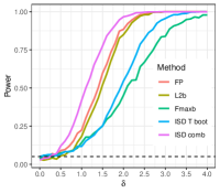
Refer to caption Refer to caption Refer to caption Refer to caption
(a) (b) (c) (d)
Figure 4: Performance on synthetic finite interval and manifold data. Finite interval: (a) comparison with existing methods—a test based on basis function representation (FP) (Gorecki & Smaga, 2015), a sum-type 2subscript2\ell_{2} norm-based test (L2b) (Zhang, 2013), and a max-type test (Zhang et al., 2019) that uses the maximum of coordinate-wise F𝐹F statistic (Fmaxb); (b) unsliced vs. different settings of (L,D)𝐿superscript𝐷(L,D^{\prime}). Manifold data: (c) circular data, comparing with Fréchet ANOVA (Dubey & Müller, 2019), and the DISCO nonparametric test (Rizzo & Székely, 2010); (d) harmonic combination tests on cylindrical data for L=4𝐿4L=4. Dotted lines indicates nominal size of all tests (α=0.05𝛼0.05\alpha=0.05).
δ𝛿\delta CH CS L2N L2b FN FB Fb GPF
0 0.031 0.03 0.033 0.024 0.031 0.028 0.033 0.026
0.1 0.025 0.024 0.03 0.044 0.027 0.03 0.041 0.021
0.2 0.026 0.029 0.037 0.06 0.033 0.034 0.058 0.025
0.3 0.036 0.041 0.044 0.067 0.041 0.04 0.067 0.033
0.4 0.034 0.035 0.036 0.057 0.034 0.035 0.056 0.032
0.5 0.051 0.052 0.058 0.091 0.056 0.057 0.088 0.044
0.6 0.056 0.066 0.066 0.089 0.061 0.066 0.088 0.051
0.7 0.07 0.083 0.083 0.121 0.084 0.081 0.119 0.064
0.8 0.085 0.097 0.095 0.151 0.093 0.094 0.144 0.081
0.9 0.118 0.142 0.14 0.2 0.144 0.137 0.194 0.118
1 0.158 0.182 0.176 0.232 0.183 0.173 0.228 0.154
1.1 0.215 0.247 0.246 0.303 0.251 0.242 0.301 0.212
1.2 0.27 0.31 0.303 0.375 0.311 0.3 0.368 0.27
1.3 0.328 0.363 0.357 0.438 0.37 0.353 0.43 0.324
1.4 0.395 0.432 0.432 0.504 0.436 0.423 0.499 0.394
1.5 0.488 0.52 0.514 0.592 0.521 0.511 0.586 0.483
1.6 0.534 0.595 0.576 0.652 0.593 0.566 0.647 0.544
1.7 0.628 0.677 0.669 0.723 0.678 0.661 0.719 0.631
1.8 0.704 0.737 0.727 0.789 0.748 0.725 0.785 0.707
1.9 0.785 0.823 0.812 0.869 0.827 0.806 0.867 0.793
2 0.83 0.849 0.844 0.88 0.85 0.841 0.875 0.832
2.1 0.865 0.888 0.881 0.916 0.887 0.878 0.915 0.872
2.2 0.903 0.922 0.916 0.946 0.928 0.912 0.946 0.907
2.3 0.938 0.95 0.944 0.964 0.951 0.944 0.963 0.944
2.4 0.958 0.973 0.967 0.977 0.972 0.966 0.976 0.964
2.5 0.974 0.98 0.976 0.985 0.981 0.975 0.985 0.974
2.6 0.977 0.981 0.979 0.987 0.981 0.978 0.986 0.977
2.7 0.989 0.996 0.992 0.997 0.996 0.992 0.997 0.991
2.8 0.997 0.998 0.997 0.998 0.998 0.997 0.998 0.996
2.9 0.996 0.997 0.996 0.999 0.997 0.996 0.999 0.997
3 0.998 1 0.999 1 1 0.999 1 0.999
Table 5: Outputs for other methods in the functional curves synthetic data setting.

We also compare the p𝑝p-value combination test based on an unsliced 24-dimensional inverse CDF embedding with sliced IS𝒲2𝐼𝑆subscript𝒲2IS\mathcal{W}_{2}-based tests (Figure 3 b). We use multiple pairs of (L,D)𝐿superscript𝐷(L,D^{\prime}) values, all of them giving overall embeddings of dimension D=LD=24𝐷𝐿superscript𝐷24D=LD^{\prime}=24. The performance of an IS𝒲2𝐼𝑆subscript𝒲2IS\mathcal{W}_{2}-based test that uses slicing over only the first eigenfunction is almost as good as the unsliced version. With more eigenfunctions, the powers first improve considerably, then become similar to the unsliced version again.

Manifold domains

We consider data from distributions on circles and cylinders. For circular data, we take von Mises distributions with randomly chosen parameters as our samples. For an angle x𝑥x (measured in radians), the von Mises probability density function is given by f(x|μ,κ)=exp[κcos(xμ)](2πI0(κ))1𝑓conditional𝑥𝜇𝜅𝜅𝑥𝜇superscript2𝜋subscript𝐼0𝜅1f(x|\mu,\kappa)=\exp[\kappa\cos(x-\mu)](2\pi I_{0}(\kappa))^{-1}, where I0(κ)subscript𝐼0𝜅I_{0}(\kappa) is the modified Bessel function of order 0. We fix κ=2𝜅2\kappa=2, and use μμiN(0,0.12)𝜇subscript𝜇𝑖similar-to𝑁0superscript0.12\mu\equiv\mu_{i}\sim N(0,0.1^{2}), μνiN(δ,0.12)𝜇subscript𝜈𝑖similar-to𝑁𝛿superscript0.12\mu\equiv\nu_{i}\sim N(\delta,0.1^{2}) for samples from group 1 and 2 respectively—with δ[0,15]×π/180𝛿015𝜋180\delta\in[0,15]\times\pi/180 (i.e. 0 to 15 degrees converted to radians). As each observation vector, we take 100 random draws from each sample-specific distribution. For our embeddings, we use L=10,D=20formulae-sequence𝐿10superscript𝐷20L=10,D^{\prime}=20, and so our final embedding dimension is 10×20×2=4001020240010\times 20\times 2=400. Since the competing methods cannot handle circular geometry directly, to implement them we cut the circle into an interval. Figure 3 (c) shows that all methods maintain nominal size, but both our tests maintain considerably higher power than existing methods for all δ𝛿\delta.

We generate cylindrical data in the form of samples of a bivariate random vector (Θ,X)Θ𝑋(\Theta,X), using the cylindrical density function proposed by (Mardia & Sutton, 1978):

f(θ,x)=eκcos(θμ)2πI0(κ)12πσce(xμc)22σc2,𝑓𝜃𝑥superscript𝑒𝜅𝜃𝜇2𝜋subscript𝐼0𝜅12𝜋subscript𝜎𝑐superscript𝑒superscript𝑥subscript𝜇𝑐22superscriptsubscript𝜎𝑐2f(\theta,x)=\frac{e^{\kappa\cos(\theta-\mu)}}{2\pi I_{0}(\kappa)}\frac{1}{\sqrt{2\pi}\sigma_{c}}e^{-\frac{(x-\mu_{c})^{2}}{2\sigma_{c}^{2}}},

clipping values of the X𝑋X-coordinate between the bounded interval [0,2π]02𝜋[0,2\pi]. This distribution has the parameters μ[π,π],μ0,κ0,ρ1[0,1),ρ2[0,1),σ>0formulae-sequence𝜇𝜋𝜋formulae-sequencesubscript𝜇0formulae-sequence𝜅0formulae-sequencesubscript𝜌101formulae-sequencesubscript𝜌201𝜎0\mu\in[-\pi,\pi],\mu_{0}\in\mathbb{R},\kappa\geq 0,\rho_{1}\in[0,1),\rho_{2}\in[0,1),\sigma>0, where μ,κ𝜇𝜅\mu,\kappa denote parameters for the (circular) marginal along the ΘΘ\Theta-coordinate. and given Θ=θΘ𝜃\Theta=\theta, X𝑋X is sampled from N(μc,σc2)𝑁subscript𝜇𝑐superscriptsubscript𝜎𝑐2N(\mu_{c},\sigma_{c}^{2}), with

μcsubscript𝜇𝑐\displaystyle\mu_{c} =\displaystyle= μ+κσ{ρ1(cosθcosμ)+ρ2(sinθsinμ)},𝜇𝜅𝜎subscript𝜌1𝜃𝜇subscript𝜌2𝜃𝜇\displaystyle\mu+\sqrt{\kappa}\sigma\left\{\rho_{1}(\cos\theta-\cos\mu)+\rho_{2}(\sin\theta-\sin\mu)\right\},
σcsubscript𝜎𝑐\displaystyle\sigma_{c} =\displaystyle= σ2(1ρ2),ρ=(ρ12+ρ22)1/2.superscript𝜎21superscript𝜌2𝜌superscriptsuperscriptsubscript𝜌12superscriptsubscript𝜌2212\displaystyle\sigma^{2}(1-\rho^{2}),\rho=(\rho_{1}^{2}+\rho_{2}^{2})^{1/2}.

In our experiments, we fix ρ1=ρ2=0.5,σ=1,κ=2formulae-sequencesubscript𝜌1subscript𝜌20.5formulae-sequence𝜎1𝜅2\rho_{1}=\rho_{2}=0.5,\sigma=1,\kappa=2 across both populations. As random samples of distributions, we draw μ,μ0Unif(0,1)similar-to𝜇subscript𝜇0Unif01\mu,\mu_{0}\sim\text{{Unif}}(0,1) and μ,μ0Unif(δ,δ+1)similar-to𝜇subscript𝜇0Unif𝛿𝛿1\mu,\mu_{0}\sim\text{{Unif}}(\delta,\delta+1) for samples of group 1 and 2 respectively, with n1=60,n2=40formulae-sequencesubscript𝑛160subscript𝑛240n_{1}=60,n_{2}=40. We repeat the above for δ[0,30]𝛿030\delta\in[0,30] degrees converted to radians, and obtain bivariate histograms corresponding to each sample distribution from 500 random draws from that distribution. To evaluate the effects of choosing L,D𝐿superscript𝐷L,D^{\prime} we calculate our embeddings for L{2,3,4,5},D{6,8,12,24,48}formulae-sequence𝐿2345superscript𝐷68122448L\in\{2,3,4,5\},D^{\prime}\in\{6,8,12,24,48\}. The choice of L𝐿L has small effect on performance, so we report results for L=4𝐿4L=4 in Figure 3 (d). Higher values of Dsuperscript𝐷D^{\prime} result in some increase in power.

Discussion

Our IS𝒲2𝐼𝑆subscript𝒲2IS\mathcal{W}_{2}-based method is able to exploit the non-euclidean nature of the problems and and their generality beyond mean comparison more effectively than competing methods, which are based on mean comparison on functional data/densities (frechet ANOVA, all functional ANOVA methods), and/or L2 distance-based comparisons (all functional ANOVA methods, DISCO). Regarding the optimal choice of embedding dimensions, while proving theorem 5.1 we show that (Proposition 10 therein) choosing both L𝐿L and D𝐷D above certain thresholds ensures close approximation to the population test statistic. For the combination test, adding more dimensions to the embedding can have a two-fold effect: a) probing more dimensions can help with finding differences, but b) every dimension adds another test and so potentially leads to loss of power. Thus, for the combination test, there must be an optimal data dependent choice of the embedding dimension, which can potentially be found via split testing procedures. We leave this to future work.

Computational Complexity

Assume an underlying graph G=(V,E)𝐺𝑉𝐸G=(V,E), and we use L𝐿L slices, Dsuperscript𝐷D^{\prime} quantiles to calculate IS𝒲2𝐼𝑆subscript𝒲2IS\mathcal{W}_{2}. Each distribution consists of V𝑉V atoms (distribution lives on graph vertices). Then, computation of our embeddings includes the following steps:

  1. 1.

    The computation of eigenvectors/values of symmetric sparse matrices is a well-studied problem with stable and efficient algorithms available, e.g. ARPACK providing an implementation of the Arnoldi method in MATLAB, Python, or R. These methods incur linear time complexity in the size of graph: O(L(|V|+|E|)O(L(|V|+|E|). This computation is done only once per domain, and the overhead is negligible (<<1much-less-thanabsent1<<1 second) for our graph experiments.

  2. 2.

    Hilbert embedding computations require computing L𝐿L pushforwards and Dsuperscript𝐷D^{\prime} quantiles, which need sorting. This complexity is O(L(|V|log|V|+|D|)O(L(|V|\log|V|+|D^{\prime}|).

  3. 3.

    Testing using p-value combination requires computing t-test p-values for LD𝐿superscript𝐷LD^{\prime} dimensions, with overall complexity of O(LDN)𝑂𝐿superscript𝐷𝑁O(LD^{\prime}N) where N𝑁N is total sample size.

In contrast, Sobolev Transport (ST) requires computing the Sliced ST Distance, based on computing shortest paths from randomly selected nodes in a graph. This has complexity O(k(|V|log|V|+|E|)O(k(|V|\log|V|+|E|) (Le et al., 2022, pg. 4) Implementing permutation tests means repeating the above computation P𝑃P times, with P=1000𝑃1000P=1000 being a typical choice.

B.2 NHANES data on physical activity monitoring

As our first real data application, we analyze the Physical Activity Monitor (PAM) data from the 2005-2006 National Health and Nutrition Examination Survey (NHANES)222https://wwwn.cdc.gov/Nchs/Nhanes/2005-2006/PAXRAW_D.htm. This contains physical activity pattern readings for a large number of people collected over 1 week period on a per-minute granularity. After basic pre-processing steps to ensure no missing entries, as well as data reliability and well-calibrated activity monitors, we use data from 6839 individuals. The data for each individual corresponds to device intensity value from the PAM for 24×60=14402460144024\times 60=1440 minutes throughout the day, for 7 days.
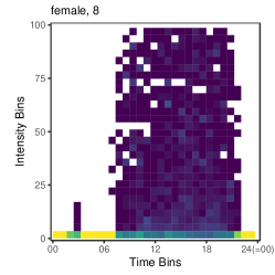
Refer to caption Refer to caption Refer to caption Refer to caption
Figure 5: Activity histograms for three individuals from NHANES dataset. There are 100 bins in the intensity and 96 in the time dimension; we show hour of day on the time axis. The time dimension is periodic where 00:00 is identified with 24:00, giving rise to a cylindrical histogram domain.
Refer to caption Refer to caption Refer to caption Refer to caption
Figure 6: Three eigenfunctions for the NHANES histogram domain normalized by the maximum absolute value. Note that the eigenfunctions are periodic in the time direction (i.e. match when glued over the side cut) but not in the intensity direction, reflecting the cylindrical geometry of the underlying domain.

For each individual we can capture their activity patterns into a cylindrical histogram with time and intensity dimensions. For each observation, its time during the day is discretized into 15-minute intervals giving 96 bins for the time dimension; its intensity value (capped at 1,000) is discretized into a 100 equidistant bins. Since the time dimension is periodic, we obtain a histogram over the cylinder S1(T1)×[0,T2)superscript𝑆1subscript𝑇10subscript𝑇2S^{1}(T_{1})\times[0,T_{2}), with T1=96,T2=100formulae-sequencesubscript𝑇196subscript𝑇2100T_{1}=96,T_{2}=100. Normalized counts can thus be considered as person-specific probability distributions; several examples are shown in Figure 5. Note that flattening the domain by cutting the cylinder will arbitrarily split activity patterns (see especially Figure 5, Female 37) and will lead to inefficiencies due to horizontal variability.

We apply the proposed methodology to check if the activity patterns vary across different groups of individuals obtained as follows. We first split the overall dataset based on the individual’s age using the following inclusive ranges: 6–15, 16–25, …,76–85; this covers all the ages in the dataset. From each split we sample 100 males and 100 females to avoid gender imbalance driving the results. Thus, we end up with 8 age groups with 200 individuals per group. Our goal is to compare these 8 groups’ activity patterns by conducting pair-wise tests.

To perform our analysis we compute the eigenvalues and eigenfunctions as per the 4th row of Table 4 using 1=1,2,3subscript1123\ell_{1}=1,2,3 and 2=1,2,3subscript2123\ell_{2}=1,2,3, giving a total of L=2×3×3=18𝐿23318L=2\times 3\times 3=18 eigenfunctions; three of the resulting eigenfunctions are shown in Figure 6. We consider a D=5superscript𝐷5D^{\prime}=5 dimensional embedding for the inverse CDF transformation, hence the final embedding dimension after the slicing construction is D=LD=18×5=90𝐷𝐿superscript𝐷18590D=LD^{\prime}=18\times 5=90.

We summarize the results in Table 6, below the diagonal. The p𝑝p-values are obtained via the harmonic mean combination approach. We run the Benjamini-Hochberg (Benjamini & Hochberg, 1995) procedure on the resulting p𝑝p-values at the false discovery rate of 0.10.10.1, and the rejected hypotheses are indicated by the p𝑝p-values in bold. Our method detects statistically significant differences between all pairs of groups, except 46–55 versus 36–45 and 56-65 groups. As a control experiment, we provide our method with null cases and display the p𝑝p-values in Table 6, above the diagonal. The null cases are obtained by combining the individuals from the two comparison groups and splitting it arbitrarily (i.e. mixing the two age groups). As expected, the p𝑝p-values of the control comparisons do not concentrate near zero.

Age Groups 6–15 16–25 26–35 36–45 46–55 56–65 66–75 76–85
6–15 0.979 0.31 0.383 0.297 0.905 0.921 0.326
16–25 3.7e-11 0.998 0.963 0.443 0.872 0.442 0.529
26–35 4.6e-20 1.0e-05 0.987 0.818 0.93 0.731 0.992
36–45 3.2e-26 3.5e-11 0.01 0.945 0.984 0.974 0.327
46–55 6.6e-27 8.4e-16 0.002 0.377 0.832 0.618 0.844
56–65 2.4e-32 7.5e-20 3.1e-04 0.042 0.977 0.509 0.98
66–75 5.4e-45 1.6e-16 7.7e-06 1.6e-04 0.001 0.011 0.557
76–85 3.4e-52 1.4e-23 1.4e-15 2.7e-12 9.7e-16 1.4e-09 2.1e-06
Table 6: Comparing the activity intensity of different age groups based on the NHANES dataset. Below diagonal: p𝑝p-values corresponding to the actual data comparisons. Above diagonal: null p𝑝p-values obtained by combining and randomly splitting the two involved groups. The entries in boldface correspond to the rejected hypotheses with the BH procedure at the FDR level of 0.1.

Curiously, our method can be used “off-label” to conduct functional data analyses over different dimensions of the NHANES dataset. For example, one can concentrate on a single day of activity intensity data which gives a curve over the 24-hour circle. Since activity intensity is a non-negative number, these curves can be normalized so as to obtain probability distributions. Now we can use our methodology to detect pair-wise differences across groups. While this has the benefit of accounting for underlying geometry of data, it loses the absolute magnitude information due to the normalization. Clearly the appropriateness of such an analysis would depend on the goal of the exercise and the particular research question attached to that goal; our proposal provides a framework that is flexible enough to handle data of different modalities.

B.3 Chicago Crime
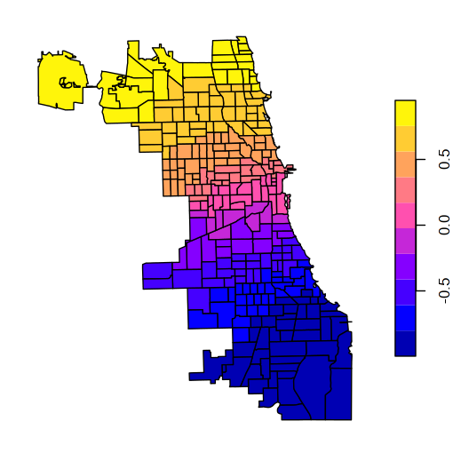
Refer to caption Refer to caption Refer to caption
(a) ϕ1()subscriptitalic-ϕ1\phi_{1}(\cdot) (b) ϕ2()subscriptitalic-ϕ2\phi_{2}(\cdot) (c) ϕ3()subscriptitalic-ϕ3\phi_{3}(\cdot)
Figure 7: First three eigenvectors of the Laplacian are shown for the beat adjacency graph, mapped back to the geographic locations. All of the eigenvectors are normalized by the maximum absolute value. The spatial smoothness of the eigenvectors—somewhat masked here due to the discrete colormap—is crucial to efficiently capturing horizontal variability of the data (i.e. distribution shifts over the graph). The boundaries of beats are shown based on the shape file from Chicago Data portal.

We demonstrate the use of our methodology on histograms over graphs. In this experiment, we use the Chicago Crimes 2018 dataset333data.cityofchicago.org which captures incidents of crime in the City of Chicago. We base our analysis on the type of crime, the beat (geographic area subdivision used by police, see Figure 7) where the incident took place, and the date of the incident. To capture the spatial aspect of the data we build a graph with one vertex per beat; two vertices are connected by an edge if the corresponding beats share a geographic boundary. For each crime type and day, we capture the total count of that crime type for each beat; after normalizing this gives a daily probability distribution over the graph. Our goal is to compare the collection of distributions of, say, theft occurring on Tuesday to those of Thursday and Saturday. The Tuesday versus Thursday comparison is intended as a null case, as we do not expect to see any differences between them (Rustamov & Klosowski, 2020).

We build the un-normalized Laplacian of the beat adjacency graph, and compute its lowest frequency L=20𝐿20L=20 eigenvalues and eigenvectors. The first three eigenvectors are plotted in Figure 7. The number of inverse CDF values used in the embedding is D=5superscript𝐷5D^{\prime}=5, which gives rise to D=100𝐷100D=100 dimensional embedding. The results of comparisons are shown in the last two columns of Table 7; the p𝑝p-values are obtained via the harmonic mean combination approach. We run the Benjamini-Hochberg (Benjamini & Hochberg, 1995) procedure on the 20 resulting p𝑝p-values at the false discovery rate of 0.10.10.1, and the rejected hypotheses are indicated by the p𝑝p-values in bold. As expected, no differences were detected between Tuesday and Thursday patterns. On the other hand, we see that there are statistically significant differences between Tuesday and Saturday patterns in the following categories of crime: theft, deceptive practice, battery, robbery, narcotics, and criminal damage.

Crime Type Tuesday Thursday Saturday Tue vs Thu Tue vs Sat
N𝑁N count¯¯count\mathrm{\overline{count}} N𝑁N count¯¯count\mathrm{\overline{count}} N𝑁N count¯¯count\mathrm{\overline{count}} p𝑝p-value p𝑝p-value
Theft 52 178.7 52 182.9 52 180.2 0.452 4.7e-06
Deceptive Practice 51 55.8 52 54.9 52 44.4 0.255 4.2e-04
Battery 52 125.8 52 123.0 52 154.9 0.374 0.001
Robbery 50 25.2 50 25.1 52 28.1 0.130 0.002
Narcotics 51 36.0 51 34.6 50 36.9 0.890 0.008
Criminal Damage 52 70.0 52 73.7 52 83.0 0.901 0.03
Other Offense 52 49.5 52 48.4 52 44.1 0.670 0.037
Burglary 52 34.0 52 33.1 52 29.1 0.157 0.183
Motor Vehicle Theft 52 27.9 52 26.2 51 28.1 0.923 0.365
Assault 52 57.2 52 59.3 52 52.4 0.996 0.617
Table 7: Results on Chicago Crime 2018 dataset. The entries in bold correspond to the rejected hypotheses with the BH procedure at the FDR level of 0.1. The N𝑁N column captures the number of days passing the filtering criteria, and the count¯¯count\mathrm{\overline{count}} column shows the average per-day crime count.

B.4 Brain Connectomics

In this example, we consider two publicly available brain connectomics datasets (Aine et al., 2017; Arroyo Relión et al., 2019) distributed as a part of the R package graphclass444http://github.com/jesusdaniel/graphclass. Both are based on resting state functional magnetic resonance imaging (fMRI): COBRE has data on 54 schizophrenics and 70 controls, and UMich with 39 schizophrenics and 40 controls. The datasets capture the pairwise correlations between 264 regions of interest (ROI) of Power parcellation (Power et al., 2011) and can be considered as a 264 node graph (263 nodes for COBRE as ROI 75 is missing) with positive and negative edge weights.

We define three probability measures supported on the nodes of the graph. For each ROI we take the sum of absolute values of all its correlations with the remaining ROIs. Now we have a positive number assigned to each node capturing its overall connectivity to the rest of the graph and we normalize to obtain a measure; this construction will be referred to as “all correlations”. Note that each scanned subject gives rise to a separate “all correlations” probability measure on the same underlying node set. The “positive correlations” and “negative correlations” constructions are based on keeping respectively only positive or only negative correlations and aggregating as above.

We also need a fixed base graph for the computation of the Laplacian eigen-decomposition; this graph should capture the spatial connectivity of the ROIs which is relevant due to the smooth nature of the blood oxygenation level dependent (BOLD) signal that is used for computing the correlations. To this end, we obtain the coordinates for the centers of the 264 ROIs555www.jonathanpower.net/2011-neuron-bigbrain.html and build the base graph by connecting each ROI to its nearest 8 ROIs.We compute the lowest frequency L=20𝐿20L=20 eigenvalues and eigenvectors of the corresponding un-normalized Laplacian. The number of inverse CDF values used in the embedding is D=5superscript𝐷5D^{\prime}=5, which gives rise to D=100𝐷100D=100 dimensional embedding.

Dataset All correlations Positive correlations Negative correlations
COBRE 0.0084 0.00019 0.0019
UMich 0.609 0.116 0.022
Table 8: Comparison results between the schizophrenic and control groups for brain connectomics datasets.

Table 8 shows the result of comparing the schizophrenic group to the control group for both of the datasets; the p𝑝p-values are obtained via the harmonic mean combination approach. We can see that our approach detects statistically significant differences between the two groups in COBRE dataset in all of the three types of measures on graphs. In contrast, for UMich dataset, the difference is detected only in the negative correlations and loses significance when corrected for multiple testing. This is potentially caused by the higher inhomogeneity of the UMich dataset that was pooled across five different experiments spanning seven years (Arroyo Relión et al., 2019). An interesting aspect of our analysis is that due to normalization (to obtain probability measures) the total sum of connectivity is factored out by the proposed method. As a result, the detected differences are not related to the well-known change in the overall connectivities between the two groups, but rather to distributional changes in marginal connectivity strengths.