Lin, Ma, Nadarajah, Soheili

A Restarting Level Set Method

A Parameter-free and Projection-free Restarting Level Set Method for Adaptive Constrained Convex Optimization Under the Error Bound Condition

Qihang Lin The University of Iowa, Tippie College of Business,
qihang-lin@uiowa.edu Runchao Ma The University of Iowa, Tippie College of Business,
runchao-ma@uiowa.edu Selvaprabu Nadarajah University of Illinois at Chicago, College of Business Administration,
selvan@uic.edu Negar Soheili University of Illinois at Chicago, College of Business Administration,
nazad@uic.edu

Recent efforts to accelerate first-order methods have focused on convex optimization problems that satisfy a geometric property known as error-bound condition, which covers a broad class of problems, including piece-wise linear programs and strongly convex programs. Parameter-free first-order methods that employ projection-free updates have the potential to broaden the benefit of acceleration. Such a method has been developed for unconstrained convex optimization but is lacking for general constrained convex optimization. We propose a parameter-free level-set method for the latter constrained case based on projection-free subgradient decent that exhibits accelerated convergence for problems that satisfy an error-bound condition. Our method maintains a separate copy of the level-set sub-problem for each level parameter value and restarts the computation of these copies based on objective function progress. Applying such a restarting scheme in a level-set context is novel and results in an algorithm that dynamically adapts the precision of each copy. This property is key to extending prior restarting methods based on static precision that have been proposed for unconstrained convex optimization to handle constraints. We report promising numerical performance relative to benchmark methods.

level set method, parameter free, projection free, accelerated methods, constrained convex optimization, error bound condition

1 Introduction.

In this paper, we consider a convex optimization problem with inequality constraints:

$$f^{*}:=\min_{{\mathbf{x}}\in\mathcal{X}}\{f({\mathbf{x}}):=f_{0}({\mathbf{x}})\quad\text{s.t.}\quad g({\mathbf{x}}):=\max_{i=1,\dots,m}f_{i}({\mathbf{x}})\leq 0\},$$ (1)

where $f_{i}$ for $i=0,1,\dots,m$ are convex real-valued functions and $\mathcal{X}\subset\mathbb{R}^{n}$ is a closed convex set onto which the projection mapping is easy to compute. Given $\epsilon>0$, we say a solution $\bar{\mathbf{x}}$ to (1) is $\epsilon$-optimal if $f(\bar{\mathbf{x}})-f^{*}\leq\epsilon$ and $\epsilon$-feasible if $\bar{\mathbf{x}}\in\mathcal{X}$ and $g(\bar{\mathbf{x}})\leq\epsilon$. There has been a large volume of literature on constrained convex optimization problems in deterministic settings [1, 2, 9, 14, 22, 23, 35, 36, 37, 38, 47] and significant, but comparatively less, activity in stochastic [21, 24, 47] settings.

Recent developments have focused on accelerating first order methods with linear convergence rates (without assuming strong convexity) based on a more general geometric property known as “error bound condition (EBC)”, which is

$$\dfrac{\text{dist}({\mathbf{x}},\mathcal{X}^{*})^{d}}{G}\leq\max\{f({\mathbf{x}})-f^{*},g({\mathbf{x}})\},\quad\forall{\mathbf{x}}\in\mathcal{X},$$ (2)

for some parameters $G>0$ and $d\geq 1$, where $\mathcal{X}^{*}$ is the set of optimal solutions to (1) and $\text{dist}({\mathbf{x}},\mathcal{X}^{*})$ denotes the Euclidean distance of ${\mathbf{x}}$ to $\mathcal{X}^{*}$, which we refer to as solution distance. EBC provides a lower bound on the maximum of the optimality $(f(x)-f^{*})$ and feasibility $(g(x))$ gaps as a function of the solution distance, $d$, and $G$. A larger such lower bound is desirable as it implies that additional iterations that bring ${\mathbf{x}}$ closer to $\mathcal{X}^{*}$ are needed in the pursuit of an $\epsilon$-optimal and $\epsilon$-feasible solution. In contrast, if this lower bound is very small, iterations that move ${\mathbf{x}}$ closer to $\mathcal{X}^{*}$ may not result in significant optimality or feasibility progress. Smaller values of $G$ lead to larger lower bounds all else being the same and are thus preferred. For a fixed $G$, we prefer a smaller $d$ because it corresponds to more favorable geometry closer to the optimal solution set, which is typically when the progress of first-order methods slows down. Specifically, when ${\mathbf{x}}$ is close to the set of optimal solutions (i.e., is $\text{dist}({\mathbf{x}},\mathcal{X}^{*})<1$), smaller $d$ leads to a larger lower bound. Piece-wise linear and strongly convex programs satisfy EBC for $d=1$ and $d=2$, respectively. We refer to an algorithm as adaptive if its convergence rate improves (i.e., it accelerates) as $d$ and $G$ become smaller.

Adaptive methods for unconstrained or simply constrained convex optimization problems have been explored. Almost all of them use in their step length [4, 7, 15, 17, 18, 20, 26, 30, 33, 35, 43, 48, 49] or in the frequency with which they restart [5, 6, 10, 11, 16, 25, 34, 39, 40, 41, 42, 44, 45] knowledge of $d$, $G$, and $f^{*}$. Such parameters are unknown in general and their accurate estimation is challenging. Adaptive algorithms that are also parameter free (i.e., do not rely on the knowledge of unknown parameters) would therefore broaden or ease the applicability of accelerated methods. To the best of our knowledge, [8, 19, 32] are the only parameter-free adaptive methods that handle unconstrained problems. The method in [32] employs a subgradient scheme to solve $K$ copies of the problem with termination precisions $2^{k}\epsilon$ for $k=-1,0,\ldots,K-1$. Copy $k$ communicates its current solution to copy $k-1$ when a restart is triggered. Since the copies are based on pre-defined precision, this restarting subgradient method (RSG) can be interpreted as a static precision-based restarting scheme. A key feature of RSG is that it tracks the reduction in the objective function (i.e., progress made) to determine when to trigger a restart, as opposed to relying on the distance from $f^{*}$ (i.e., remaining progress). However, RSG is not designed to handle convex optimization problems with (potentially) complicated constraints. This method has been adapted to bundle methods in [8]. [19] applies a similar idea for smooth unconstrained convex optimization problems where the restarts are triggered based on the norm of proximal gradients. There is limited work ([31], [46]) on utilizing EBC for solving the constrained convex optimization problem (1). The work in [31] considers the case of $d=1$ and their algorithm relies on knowledge of $f^{*}$. The method in [46] is for general $d$ but requires the knowledge of $G$ and $d$, among other parameters, and requires a projection on $\mathcal{X}\cap\{{\mathbf{x}}|g(x)\leq 0\}$, which is hard.

The goal of our paper is to develop an adaptive method for convex optimization with general convex constraints that is both parameter-free and projection-free. Extending RSG to handle general convex constraints would be the natural first avenue to consider to achieve our goal. Indeed, the $k$-th copy in such an extension will solve the problem of finding an $2^{k}\epsilon$-optimal and $2^{k}\epsilon$-feasible solution, which entails balancing optimality and feasibility by defining a single objective. Defining such an objective is possible given optimal Lagrange multipliers or $f^{*}$, which are both unknown. Thus extending RSG in this manner appears to be challenging.

	Smooth	Algorithm
EBC	Functions	parameters	Convergence rate
General [This paper]	No	None	$\mathcal{O}\left((M^{2}G^{(2/d)})/\epsilon^{(2-2/d)}\log^{3}(1/\epsilon)\right)$
	Yes	None	$\mathcal{O}\left(\left((MG^{(1/d)})/\epsilon^{(1-1/d)}+(\sqrt{L}G^{(1/d)})/\epsilon^{(1/2-1/d)}\right)\log^{3}(1/\epsilon)\right)$
General [46]††	No	$d$, $G$, $M$	$\mathcal{O}\left((M^{4}G^{(2/d)})/\epsilon^{(2-2/d)}\log\left(1/\epsilon\right)\right)$
	Yes	$d$, $G$, $M$, $L$	$\mathcal{O}\left((M^{2}G^{(1/d)})/\epsilon^{(1-1/d)}\log\left(1/\epsilon\right)+(\sqrt{ML}G^{(1/d)})/\epsilon^{(1-1/d)}\right)$
$d=2$ [23, 24]	No	$M$, $\mu$	$\mathcal{O}\left(M^{2}/\mu\epsilon\right)$
	Yes	$M$, $L$, $\mu$	$\mathcal{O}\left(M/\sqrt{\mu\epsilon}+\sqrt{L/\mu}\log\left(1/\epsilon\right)\right)$
$d=2$ [38]	Yes	$M$, $L$, $\mu$	$\mathcal{O}\left(\left((M+\sqrt{ML})/\epsilon+\sqrt{L/\epsilon}\right)\log(1/\epsilon)\right)$
$d=1$ [31]	No	$f^{*}$	$\mathcal{O}\left(G^{2}\log(1/\epsilon)\right)$

Table 1: Convergence rate of the subgradient methods that accelerate under the error bound condition (2) for smooth and non-smooth constrained convex optimization problems, where $M$ denotes an upper bound on the sub-gradient norm, and $L$ and $\mu$ are the smoothness (Lipschitz constant) and strong convexity parameters associated with the functions $f_{i}$, $i=0,1,\ldots,m$. ^†† indicates that the paper requires projection on $\mathcal{X}\cap\{{\mathbf{x}}|g(x)\leq 0\}$.

We show that our goal can be achieved by developing a restarting level set method. Level-set methods [1, 22, 23, 24] convert the solution of the constrained optimization problem (1) into the solution of a sequence of unconstrained non-smooth optimization problems that depend on a scalar, referred to as the level parameter. The level parameter is chosen by approximately solving a one-dimensional root-finding problem . [1] provides a detailed discussion and complexity analysis of the level set approach. Subgradient algorithms to solve the aforementioned level-set subproblems are desirable as they are easy to implement. However, level set methods that leverage subgradient algorithms depend on unknown parameters, which may include an upper bound on the subgradient norm and/or a smoothness parameter [22, 23, 24]. Our contributions are the following:

• We introduce a restarting level set method (RLS) that is both parameter-free and projection-free. It maintains $K$ copies, each distinguished by a level parameter and its associated sub-problem. Each restart of copy $k$ results in an update of the level parameters associated with copies $k,k+1,\ldots,K$. The restart of a copy is triggered by the progress made on the sub-problem objective. To the best of our knowledge, this is the first level set method based on projection-free subgradient oracles that is parameter-free, and is therefore of independent interest to the literature on level set methods.

• RLS can be interpreted as a restarting scheme with dynamic precision, which is conceptually different from RSG. To elaborate, a fixed level parameter implicitly sets a precision for a subproblem. Since RLS updates the level parameter of multiple copies in every restart, it dynamically and implicitly updates the precision associated with copies. Our key algorithmic insights are that (i) triggering restarts based on the progress of the subproblem objective and (ii) dynamically changing the precision of subproblems at each restart by updating the level parameters side step the issues discussed earlier of extending RSG to handle general constrained convex optimization.

• We establish that RLS is adaptive in addition to being parameter-free, that is, RLS exhibits acceleration under EBC. Its complexity for non-smooth problems is $\mathcal{O}((M^{2}G^{2/d})/\epsilon^{(2-2/d)}\log^{3}(1/\epsilon))$. The adaptive method in [46] has a complexity of $\mathcal{O}((M^{4}G^{2/d})/\epsilon^{2-2/d}\log(1/\epsilon))$ but it depends on unknown parameters and requires a non-trivial projection onto $\mathcal{X}\cap\{{\mathbf{x}}|g(x)\leq 0\}$. The additional $\log^{2}\left(\frac{1}{\epsilon}\right)$ factor in the RLS complexity can be interpreted as the cost of both relaxing parameter dependence and employing simple subgradient oracles. Despite this worsening, the dependence of RLS on $M$ is better. Table 1 shows that an analogous property holds in the smooth setting when comparing RLS with the approach in [46]. Although perhaps unfair to RLS, Table 1 also compares its complexity to algorithms designed for specific values of $d$, all of which depend on unknown parameters. RLS worsens by the same logarithmic factor of $\log^{2}\left(\frac{1}{\epsilon}\right)$ relative to these more specialized algorithms and sometimes improves on the dependence with respect to $G$.

• We numerical test the performance of RLS on a synthetic linear program and a classification problem with fairness constraints. We are able to vary $G$ in the synthetic linear program and confirm numerically that the number of RLS iterations to find an $\epsilon$-optimal and $\epsilon$-feasible solution increases with $G$ and $1/\epsilon$. For the classification problem with fairness constraints, we compare RLS against three parameter-free but non-adaptive benchmarks, which include the feasible level set method in [23], the subgradient method in [47], and the switching subgradient method in [2]. We find that the adaptive-nature of RLS leads to significantly faster convergence to an $\epsilon$-optimal and $\epsilon$-feasible solution than the three benchmarks.

This paper is organized as follows: In Section 2, we discuss a general level-set method for solving (1) and discuss its convergence rate. In Section 3, we present RLS and analyze its oracle complexity. In Section 4, we provide first order oracles for use with RLS in the non-smooth and smooth settings, also analyzing the iteration complexity of RLS in each case. In Section 5, we numerically compare RLS to other benchmarks. We conclude in Section 6.

2 Level set method.

Throughout the paper, we assume that there exists a computable feasible solution to (1) that strictly satisfies the constraint $g({\mathbf{x}})\leq 0$. This assumption is formalized below. There exists a computable solution $\tilde{{\mathbf{x}}}$ such that $\tilde{{\mathbf{x}}}\in\mathcal{X}$ and $g(\tilde{{\mathbf{x}}})<0$.

We define the level-set function corresponding to (1) as:

$$H(r):=\min_{{\mathbf{x}}\in\mathcal{X}}P({\mathbf{x}};r),$$ (3)

where $r\in\mathbb{R}$ is called a level parameter and

$$P({\mathbf{x}};r):=\max\{f_{0}({\mathbf{x}})-r,f_{1}({\mathbf{x}}),\dots,f_{m}({\mathbf{x}})\}=\max\{f({\mathbf{x}})-r,g({\mathbf{x}})\}.$$ (4)

Below, we summarize some of the well-known properties of $H(r)$ that we use in our algorithm and analyses.

Lemma 2.1 ([23, 29])

The function $H(r)$ defined in (3) has the following properties:

1. $H(r)$ is non-increasing and convex in $r$;

2. $H(f^{*})=0$;

3. $H(r)>0$ when $r<f^{*}$ and $H(r)\leq 0$ when $r>f^{*}$. If Assumption 2 holds, $H(r)<0$ when $r>f^{*}$;

4. $H(r)-\delta\leq H(r+\delta)\leq H(r)$ for any $\delta\geq 0$.

Lemma 2.1 indicates that $f^{*}$ is the unique root to the root-finding problem $H(r)=0$ under Assumption 2. Moreover, as shown in Lemma 2.2, it is possible to find an $\epsilon$-feasible solution and use the level parameter $r$ to bound the optimality gap.

Lemma 2.2

Given $\epsilon>0$, if ${\mathbf{x}}\in\mathcal{X}$ satisfies $P({\mathbf{x}};r)\leq\epsilon$ for some $r$, then ${\mathbf{x}}$ is $(r-f^{*}+\epsilon)$-optimal and $\epsilon$-feasible. Consequently, when $r<f^{*}$, this solution ${\mathbf{x}}$ is $\epsilon$-optimal and $\epsilon$-feasible.

Hence to tackle (1), a level-set method applies a root-finding scheme to solve $H(r)=0$ with the goal of finding $r=f^{*}$. Once such $r$ is found, then $P({\mathbf{x}};r)\leq\epsilon$ implies that ${\mathbf{x}}$ is a nearly optimal and nearly feasible solution to (1). Notice that for any ${\mathbf{x}}^{*}\in\mathcal{X}^{*}:=\argmin_{{\mathbf{x}}\in\mathcal{X}}P({\mathbf{x}};f^{*})$ we have $P({\mathbf{x}}^{*};f^{*})=0$.

Algorithm 1 presents a level set method that generates a sequence of level parameters $\{r_{k}\}_{k\geq 0}$ converging to $f^{*}$. Given $\alpha\in(0,1)$, each update of $r_{k+1}=r_{k}+\alpha P({\mathbf{x}}_{k};r_{k})$ requires a vector ${\mathbf{x}}_{k}\in\mathcal{X}$ satisfying $\alpha P({\mathbf{x}}_{k};r_{k})<f^{*}-r_{k}$, that is, condition (5). The convergence of Algorithm 1 relies on $r_{k}<f^{*}$. Under this condition, it follows from Lemma 2.1(4) and $\alpha<1$ that ${\mathbf{x}}_{k}$ can be computed by solving $\min_{{\mathbf{x}}\in\mathcal{X}}P({\mathbf{x}};r_{k})$ because $\min_{{\mathbf{x}}\in\mathcal{X}}P({\mathbf{x}};r_{k})=H(r_{k})\leq f^{*}-r_{k}<(f^{*}-r_{k})/\alpha$. Moreover, the level parameter $r_{k}$ converges to $f^{*}$ from below causing the quantity $P({\mathbf{x}}_{k};r_{k})\geq 0$ to converge to zero. Thus, Algorithm 1 terminates and the final solution is both $\epsilon$-optimal and $\epsilon$-feasible by Lemma 2.2.

Algorithm 1 Level Set Method

1:Input: $\alpha\in(0,1)$, $\epsilon>0$, and $r_{0}<f^{*}$.

2:Initialize: $k=-1$.

3:do

4:     $k=k+1$.

5:     Solve $\min_{{\mathbf{x}}\in\mathcal{X}}P({\mathbf{x}};r_{k})$ to obtain ${\mathbf{x}}_{k}\in\mathcal{X}$ such that

$$\alpha P({\mathbf{x}}_{k};r_{k})<f^{*}-r_{k}.$$ (5)

6:     Set $r_{k+1}=r_{k}+\alpha P({\mathbf{x}}_{k};r_{k})$.

7:while $P({\mathbf{x}}_{k};r_{k})\leq\epsilon$.

8:Output: ${\mathbf{x}}_{k}$.

Next, we present analysis that shows the correctness and complexity of Algorithm 1. This analysis depends on a condition measure that is defined as

$$\theta:=-\lim_{r\rightarrow f^{*-}}\frac{H(r)-H(f^{*})}{r-f^{*}}=\lim_{r\rightarrow f^{*-}}\frac{H(r)}{f^{*}-r}.$$ (6)

The following lemma sheds light on some geometric properties of the condition measure $\theta$. We skip proving this lemma as it directly follows from the definition of $\theta$ in (6) and the first and fourth properties in Lemma 2.1.

Lemma 2.3

It holds that $0<\theta\leq\dfrac{H(r)}{f^{*}-r}\leq 1$ for any $r<f^{*}$ and $0\leq\dfrac{H(r)}{f^{*}-r}\leq\theta$ for any $r>f^{*}$.

Lemma 2.3 establishes bounds on $H(r)$. In particular, when $r_{k}$ is less than $f^{*}$, there is a natural lower bound of zero.

If $r_{0}<f^{*}$, Lemma 2.4 shows that $r_{k}$ remains less than $f^{*}$ at each iteration of Algorithm 1 and that it converges to $f^{*}$ at a geometric rate.

Lemma 2.4

Suppose ${\mathbf{x}}_{k}\in\mathcal{X}$ and $r_{k}$ satisfy $r_{k}<f^{*}$ and (5). The update $r_{k+1}=r_{k}+\alpha P({\mathbf{x}}_{k};r_{k})$ in Algorithm 1 guarantees

• $r_{k+1}<f^{*}$; and

• $f^{*}-r_{k+1}\leq(1-\alpha\theta)(f^{*}-r_{k})$.

Proof 2.5

Proof. Fix $k$. Given $r_{k}$ and ${\mathbf{x}}_{k}$ satisfying $\alpha P({\mathbf{x}}_{k};r_{k})<f^{*}-r_{k}$, we have

$$r_{k+1}=r_{k}+\alpha P({\mathbf{x}}_{k};r_{k})<r_{k}+f^{*}-r_{k}=f^{*}.$$

In addition, it follows that

$$f^{*}-r_{k+1}=f^{*}-r_{k}-\alpha P({\mathbf{x}}_{k};r_{k})\leq f^{*}-r_{k}-\alpha H(r_{k})\leq\left(1-\alpha\theta\right)(f^{*}-r_{k}),$$ (7)

where the first inequality holds because $0\leq H(r_{k})\leq P({\mathbf{x}}_{k};r_{k})$ and the second one because $H(r_{k})\geq\theta(f^{*}-r_{k})$ for $r_{k}<f^{*}$ by Lemma 2.3.

In Theorem 2.6 we characterize the number of outer iterations needed by Algorithm 1 to find an $\epsilon$-optimal and $\epsilon$-feasible solution to (1).

Theorem 2.6

Given $\epsilon>0$, $\alpha\in(0,1)$, and $r_{0}<f^{*}$, Algorithm 1 terminates in at most

$$\hat{K}:=\left\lceil\frac{1}{\alpha\theta}\ln\left({\frac{f^{*}-r_{0}}{\alpha\epsilon}}\right)\right\rceil$$ (8)

iterations and returns an $\epsilon$-optimal and $\epsilon$-feasible solution to (1).

Proof 2.7

Proof. Since Algorithm 1 starts with $r_{0}<f^{*}$, Lemma 2.4 indicates that $r_{k}<f^{*}$ and (7) holds at each iteration $k\geq 0$. Since $\alpha\theta\in(0,1)$, recursively applying (7) for $k=0,1,\dots$ shows that $0\leq f^{*}-r_{k}\leq\left(1-\alpha\theta\right)^{k}(f^{*}-r_{0})$ for any $k\geq 0$. Hence, it follows from inequality (5) that $P({\mathbf{x}}_{k};r_{k})<\frac{1}{\alpha}(f^{*}-r_{k})\leq\frac{1}{\alpha}\left(1-\alpha\theta\right)^{k}(f^{*}-r_{0})$. When $k=\left\lceil\frac{1}{\alpha\theta}\ln\left({\frac{f^{*}-r_{0}}{\alpha\epsilon}}\right)\right\rceil$, we get $P({\mathbf{x}}_{k};r_{k})\leq\epsilon$ and the algorithm stops. Since $r_{k}<f^{*}$, Lemma 2.2 then guarantees that the solution ${\mathbf{x}}_{k}$ returned at termination is an $\epsilon$-optimal and $\epsilon$-feasible solution.

Remark 2.8

The $1/\theta$ factor in the definition of $\hat{K}$ arises because we leverage the natural lower bound of zero on $H(r)$, as discussed after Lemma 2.3. This choice results in the specific form of condition (5), which is a simplification of the analogous condition in [1], where the authors use non-trivial lower and upper bounds on $H(r)$. The lower bound used in [1] is easily computable only when the problem has certain structure. If such bounds can be computed efficiently, then the number of iterations taken by the algorithm in [1] does not depend on $\theta$. We choose our simpler approach because it is implementable for more general class of problems and also facilitates clearer exposition of the key ideas underlying RLS in the next section.

3 Restarting level set method.

We define a sequence of pairs $\{({\mathbf{x}}_{k},r_{k})\}_{k=0}^{K}$ with $r_{0}<f^{*}$ and ${\mathbf{x}}_{k}\in\mathcal{X}$ as a level set sequence of length $K+1$ if $r_{k+1}=r_{k}+\alpha P({\mathbf{x}}_{k};r_{k})$ holds for some $\alpha\in(0,1)$ and each $k=0,1,\dots,K-1$. It follows from Theorem 2.6 that the level set sequence generated in Algorithm 1 converges to an $\epsilon$-optimal and $\epsilon$-feasible solution when (i) ${\mathbf{x}}_{k}$ satisfies (5) and (ii) $K\geq\hat{K}$. One way to find ${\mathbf{x}}_{k}\in\mathcal{X}$ satisfying (5) is to solve the level-set subproblem (3) with $r=r_{k}$, which we denote by $\mathtt{LSP}(r_{k})$:

$$\min_{{\mathbf{x}}\in\mathcal{X}}P({\mathbf{x}};r_{k}).$$ (9)

Let $\mathtt{fom}$ represent the first-order method applied to (9). Although there are many choices for $\mathtt{fom}$, it is difficult to numerically verify (5) because $f^{*}$ is unknown. As a result, we are not able to terminate $\mathtt{fom}$ at the right time. If $\mathtt{fom}$ is terminated too soon, the returned solution ${\mathbf{x}}_{k}$ will not satisfy (5) and Algorithm 1 may not converge. If $\mathtt{fom}$ is terminated too late, Algorithm 1 will converge but consume longer run time than it actually needs.

To address this issue, we parallelize the sequential approach in Algorithm 1 by simultaneously solving multiple level-set subproblems with potentially different level parameters and restarting the solution of each such subproblem if a predetermined amount of progress in reducing its objective function has been made. We refer to this procedure as the restarting level set (RLS) method and describe its core idea next. It requires maintaining $K+1$ (with $K\geq\hat{K}$) first order method instances denoted by $\mathtt{fom}_{0},\mathtt{fom}_{1},\ldots,\mathtt{fom}_{K}$. Given ${\mathbf{x}}_{\text{ini}}\in\mathcal{X}$ and $r_{\text{ini}}<f^{*}$, we initialize the level set sequence $\{({\mathbf{x}}_{k}^{(0)},r_{k})\}_{k=0}^{K}$ with ${\mathbf{x}}_{k}^{(0)}={\mathbf{x}}_{\text{ini}}$ for $k=0,1,\dots,K$, $r_{0}=r_{\text{ini}}$, and $r_{k+1}=r_{k}+\alpha P({\mathbf{x}}_{k}^{(0)};r_{k})$ for $k=1,\dots,K-1$. We then apply $\mathtt{fom}_{k}$ to solve $\mathtt{LSP}(r_{k})$ starting from ${\mathbf{x}}_{k}^{(0)}$ for $k=0,1,\dots,K$ and denote by ${\mathbf{x}}_{k}^{(t_{k})}$ the solution computed by $\mathtt{fom}_{k}$ after $t_{k}$ iterations. The $\mathtt{fom}$ instances communicate with each other via restarts. We initiate a restart at instance $k^{\prime}$ when $P({\mathbf{x}}_{k^{\prime}}^{(0)};r_{k^{\prime}})\geq 0$ and the solution ${\mathbf{x}}_{k^{\prime}}^{(t_{k^{\prime}})}$ satisfies

$$P({\mathbf{x}}_{k^{\prime}}^{(t_{k^{\prime}})};r_{k^{\prime}})\leq BP({\mathbf{x}}_{k^{\prime}}^{(0)};r_{k^{\prime}}),$$ (10)

for a constant $B\in(0,1)$. The sequence of steps associated with restart are shown in Definition 3.1.

Definition 3.1 (Restart at $k^{\prime}$)

Set ${\mathbf{x}}_{k^{\prime}}^{(0)}={\mathbf{x}}_{k^{\prime}}^{(t_{k^{\prime}})}$ and $r_{k+1}=r_{k}+\alpha P({\mathbf{x}}_{k}^{(0)};r_{k})$ for all $k=k^{\prime},k^{\prime}+1,\ldots,K-1$. Restart $\mathtt{fom}_{k}$ from ${\mathbf{x}}_{k}^{(0)}$ for $k=k^{\prime},k^{\prime}+1,\ldots,K$.

In other words, initiating a restart at $k^{\prime}<K$, we reset $\mathtt{fom}_{k^{\prime}}$ to begin at an updated initial solution equal to ${\mathbf{x}}_{k^{\prime}}^{(t_{k^{\prime}})}$ and solve the same level set subproblem $\mathtt{LSP}(r_{k^{\prime}})$ as before the restart because $r_{k^{\prime}}$ is not updated. In contrast, for indices $k=k^{\prime}+1,\ldots,K$, $\mathtt{LSP}(r_{k})$ changes because the restart changes $r_{k}$. This new level set subproblem is solved by $\mathtt{fom}_{k}$ starting from the same initial solution ${\mathbf{x}}_{k}^{(0)}$ that was used before the restart. If a restart is initiated at $K$, we only perform the update ${\mathbf{x}}_{K}^{(0)}={\mathbf{x}}_{K}^{(t_{K})}$. Restarts initiated at index $k^{\prime}$ have no effect on $\mathtt{fom}_{k}$ for $k=0,1,\dots,k^{\prime}-1$, so those $\mathtt{fom}$s will continue their iterations. Lemma 3.2 follows from our restarting updates.

Lemma 3.2

The level set sequence $\{({\mathbf{x}}_{k}^{(0)},r_{k})\}_{k=0}^{K}$ remains a level set sequence after each restart.

Remark 3.3

We highlight that restarts dynamically modify the precision with which subproblems need to be solved by $\mathtt{fom}$ instances to satisfy (5). Specifically, the precision of a solution at instance $k$ can be viewed as the deviation of $P({\mathbf{x}}_{k}^{(t_{k})};r_{k})$ from the optimal subproblem objective of $H(r_{k})$. This difference satisfies

$$P({\mathbf{x}}_{k}^{(t_{k})};r_{k})-H(r_{k})\leq\dfrac{1}{\alpha}(f^{*}-r_{k})-\theta(f^{*}-r_{k})\leq(1-\alpha\theta)P({\mathbf{x}}_{k}^{(0)};r_{k}),$$

where the first inequality follows from Lemma 2.3 and the fact that the solution $x_{k}^{(t_{k})}$ satisfies (5) and the second inequality holds since the initial solution ${\mathbf{x}}_{k}^{(0)}$ does not satisfy (5). i.e. $\alpha P({\mathbf{x}}_{k}^{(0)};r_{k})>f^{*}-r_{k}.$ It follows from these inequalities that the precision $P({\mathbf{x}}_{k}^{(t_{k})};r_{k})-H(r_{k})$ is $\Theta(P({\mathbf{x}}_{k}^{(0)};r_{k}))$. A restart at $k^{\prime}$ changes ${\mathbf{x}}_{k}^{(0)}$ or $r_{k}$ of instances $k\geq k^{\prime}$ and hence the value of $P({\mathbf{x}}_{k}^{(0)};r_{k})$ at these instances. Therefore, RLS can be interpreted as an approach that dynamically modifies the precision required to satisfy (5) at a subset of instances, each time a restart is initiated as the result of there being sufficient progress in the subproblem objective function at some instance, that is, condition (10) is satisfied. The dynamic precision affects the choice of step sizes and smoothing parameters in the specific $\mathtt{fom}$ methods we employ in Section 4 for the non-smooth and smooth settings, respectively (see remarks 4.4 and 4.11).

Well-known choices of $\mathtt{fom}$ (e.g., subgradient decent) can be shown to meet the restart condition (10) after a finite number of iterations starting from ${\mathbf{x}}^{(0)}$ when $P({\mathbf{x}}^{(0)};r)\geq 0$ is sufficiently large. In particular, when $P({\mathbf{x}}^{(0)};r)>\epsilon$, the number of iterations taken by $\mathtt{fom}$ to find a desirable solution can be bounded by an integer $n^{\mathtt{fom}}$ that is independent of $r$ and ${\mathbf{x}}^{(0)}$. We summarize this property in Assumption 3 and take it to be true in this section. We will present $\mathtt{fom}$ choices that satisfy this assumption in §4.

Consider $\alpha$, $B$, $\epsilon$, $r$, and ${\mathbf{x}}^{(0)}\in\mathcal{X}$ such that $0<\alpha<B<1$, $\epsilon>0$, $r<f^{*}$, and $P({\mathbf{x}}^{(0)};r)>\epsilon$. There exists an $\mathtt{fom}$ initiated at ${\mathbf{x}}^{(0)}$ which guarantees that the inequality $P({\mathbf{x}}^{(t)};r)\leq BP({\mathbf{x}}^{(0)};r)$ holds after $t\leq n^{\mathtt{fom}}$ iterations if (5) is not satisfied by then, where $n^{\mathtt{fom}}$ is an integer depending on $\alpha$, $B$ and $\epsilon$ and independent of ${\mathbf{x}}^{(0)}$ and $r$.

To interpret RLS, it is useful to think of instance $\mathtt{fom}_{k}$ as being a proxy for the first order method applied to solve $\mathtt{LSP}(r_{k})$ in iteration $k$ of Algorithm 1. By Lemma 3.2, the relationship between the $r_{k}$ values across iterations $k$ in Algorithm 1 are also maintained for the $r_{k}$ values across instances $\mathtt{fom}_{k}$ in RLS but some $r_{k}$ may not be computed based on a solution that satisfies (5). As a result, even though the initial level set parameter is less than $f^{*}$, subsequent updates can push $r_{k}\geq f^{*}$. Theorem 3.4 states key properties of RLS that allows it to nevertheless converge to a near-optimal and near-feasible solution, as we will discuss shortly.

Theorem 3.4

Given $\epsilon>0$ and $\alpha\in(0,1)$, consider a level set sequence $\{({\mathbf{x}}_{k}^{(0)},r_{k})\}_{k=0}^{K}$ with $K\geq\hat{K}$ where $\hat{K}$ is defined in (8). At least one of the following two statements holds:

• There exists an index $k^{*}\in\{0,1,\dots,K\}$ such that $r_{k^{*}}<f^{*}$ and $\alpha P({\mathbf{x}}^{(0)}_{k^{*}};r_{k^{*}})\geq f^{*}-r_{k^{*}}$;

• The solution ${\mathbf{x}}^{(0)}_{K}$ is an $\epsilon$-optimal and $\epsilon$-feasible solution.

Moreover, if statement A holds, it follows that the index $k^{*}$ is unique and we have $r_{0}<\dots<r_{k^{*}}<f^{*}$ and $\alpha P({\mathbf{x}}_{k}^{(0)};r_{k})<f^{*}-r_{k}$ for $k=1,2,\ldots,k^{*}-1$.

Proof 3.5

Proof. Suppose statement A does not hold for any index $k\leq K$. We show the statement $B$ holds. By the definition of a level set sequence, we have $r_{0}<f^{*}$ and $r_{k+1}=r_{k}+\alpha P({\mathbf{x}}_{k}^{(0)};r_{k})$ for all $k$. Since $\alpha P({\mathbf{x}}_{k}^{(0)};r_{k})<f^{*}-r_{k}$ (by our assumption that $A$ does not hold), Lemma 2.4 guarantees that $r_{1}<f^{*}$. Using the same argument and by induction, Lemma 2.4 implies $r_{k}<f^{*}$ and $f^{*}-r_{k}\leq\left(1-\alpha\theta\right)^{k}(f^{*}-r_{0})$ for any $k$. Therefore, we have $P({\mathbf{x}}_{K}^{(0)};r_{K})<1/\alpha(f^{*}-r_{K})\leq\frac{1}{\alpha}\left(1-\alpha\theta\right)^{{K}}(f^{*}-r_{0})$. Since $K\geq\hat{K}$ with $\hat{K}$ defined in (8), we have $P({\mathbf{x}}_{K}^{(0)};r_{K})\leq\epsilon$ which indicates ${\mathbf{x}}_{K}^{(0)}$ is an $\epsilon$-optimal and $\epsilon$-feasible solution by Lemma 2.2.

Next we prove the rest of the conclusion. Let $k^{*}$ denote the smallest index satisfying the conditions of statement A. If $k^{*}=0$ the conclusion is trivial since $r_{0}<f^{*}$. Suppose $k^{*}>0$. Since $r_{0}<f^{*}$, following the definition of $k^{*}$, we must have $\alpha P({\mathbf{x}}_{0}^{(0)};r_{0})<f^{*}-r_{0}$. Lemma 2.4 then guarantees that $r_{1}<f^{*}$. Applying the same argument, we can show $r_{2},...,r_{k^{*}-1}$ are all less than $f^{*}$ ( i.e. $r_{k}<f^{*}$) and hence the inequality $\alpha P({\mathbf{x}}_{k}^{(0)};r_{k})<f^{*}-r_{k}$ must hold for any $k<k^{*}$. In addition, recall that $P({\mathbf{x}};r)\geq H(r)>0$ for any $r<f^{*}$. Hence, the relationship $r_{k+1}=r_{k}+\alpha P({\mathbf{x}}_{k}^{(0)};r_{k})$ shows $r_{k+1}>r_{k}$ for any $k<k^{*}$. The index $k^{*}$ in $A$ is unique because it is straightforward to see $r_{k^{*}+1}\geq f^{*}$ which follows from the definition of $r_{k^{*}+1}$ and the inequality $\alpha P(x_{k^{*}}^{(0)},r_{k^{*}})\geq f^{*}-r_{k^{*}}$. Moreover, once there exists an index $k$ such that $r_{k}\geq f^{*}$, we must have $r_{i}\geq f^{*}$ for all $i\geq k$ since

$$r_{i+1}-f^{*}=r_{i}-f^{*}+\alpha P({\mathbf{x}}_{i}^{(0)};r_{i})\geq r_{i}-f^{*}+\alpha H(r_{i})\geq(1-\alpha\theta)(r_{i}-f^{*})\geq 0,$$

where the first inequality holds by the definition of $H(\cdot)$ and the second by Lemma 2.3. Therefore, given that $r_{k^{*}+1}\geq f^{*}$, we must have $r_{k}\geq f^{*}$ for any $k\geq k^{*}+1$.

Given a level set sequence, we refer to the unique index $k^{*}$ in Theorem 3.4 as the critical index. At this index, we have $r_{k^{*}}<f^{*}$ but condition (5) does not hold. For all indices $k$ that precede the critical index, we have $r_{k}<f^{*}$ and condition (5) holds. Moreover, if $K\geq\hat{K}$ and $k^{*}$ does not exist (intuitively $k^{*}\geq K+1$), it implies the solution ${\mathbf{x}}_{K}^{(0)}$ is an $\epsilon$-optimal and $\epsilon$-feasible. Therefore, we would like to increase the critical index with restarts so that it eventually exceeds $K$. Ideally, if one could initiate restarts at the critical index $k^{*}$ sufficiently many times, it would reduce $P({\mathbf{x}}_{k^{*}}^{(0)};r_{k^{*}})$ by updating ${\mathbf{x}}_{k^{*}}^{(0)}$ while ensuring $r_{k^{*}}<f^{*}$ (since $r_{k^{*}}$ is not updated when a restart is initiated at $k^{*}$ by Definition 3.1). Then one would expect condition (5) will hold at $k^{*}$. Moreover, when this happens, $r_{k^{*}+1}<f^{*}$ by Lemma 2.4. Hence, repeated restarts at the critical index should intuitively increase its value.

Unfortunately, this intuition is of little algorithmic use since the critical index defined using $f^{*}$ is unknown. Therefore, RLS instead executes restarts at the smallest index at which condition (10) is satisfied. This index could be smaller than or greater than the critical index $k^{*}$. We refer to as desirable restarts the ones initiated at index $k$ less than or equal to $k^{*}$ because such restarts may update $r_{k^{*}}$ or ${\mathbf{x}}_{k^{*}}^{(0)}$. By Assumption 3 and Theorem 3.4, a desirable restart must be initiated at $\mathtt{fom}_{k}$ with some $k\leq k^{*}$ in no more than $n^{\mathtt{fom}}$ iterations, unless $P({\mathbf{x}}_{k^{*}}^{(0)};r_{k^{*}})\leq\epsilon$. In the latter case the solution ${\mathbf{x}}_{k^{*}}^{(0)}$ is $\epsilon$-optimal and $\epsilon$-feasible. The number of desirable restarts can be bounded by $\mathcal{O}(\log^{2}(1/\epsilon))$ as we will establish later. Such restarts that occur before $k^{*}$ may already increase the critical index. If this does not happen, desirable restarts will start happening at $k^{*}$ and increase the critical index.

Algorithm 2 formalizes the steps of RLS. The inputs to this algorithm include the number of $\mathtt{fom}$ instances $K$, a total budget $I$ on the number of $\mathtt{fom}$ iterations, a level parameter $r_{\text{ini}}<f^{*}$, a strictly feasible solution ${\mathbf{x}}_{\text{ini}}\in\mathcal{X}$, and parameters $\alpha$, $B$, and $\epsilon$. By Assumption 2, we can set ${\mathbf{x}}_{\text{ini}}=\tilde{\mathbf{x}}$. For $K$, an ideal value to use is $\hat{K}$ defined in (8). However, since the parameters $\theta$ and $f^{*}$ in this bound are unknown, we compute a bound on $\hat{K}$ by using a strictly feasible solution. In particular, we use

$$\tilde{K}:=\left\lceil\frac{1}{\alpha\tilde{\theta}(r)}\ln\left({\frac{\tilde{r}-r_{0}}{\alpha\epsilon}}\right)\right\rceil$$ (11)

with $\tilde{r}:=f(\tilde{\mathbf{x}})-g(\tilde{\mathbf{x}})$ and $\tilde{\theta}(r):=g(\tilde{\mathbf{x}})/(r-\tilde{r})$ for $r<f^{*}$ and $\tilde{\mathbf{x}}$ from Assumption 2. We show below $\tilde{K}$ is an upper bound on $\hat{K}$. We set $r=r_{\text{ini}}$ in definition of $\tilde{\theta}(r)$ when executing Algorithm 2.

Lemma 3.6

Let $\tilde{\mathbf{x}}$ be the strictly feasible solution in Assumption 2 and $\tilde{r}:=f(\tilde{{\mathbf{x}}})-g(\tilde{{\mathbf{x}}})$ and $\tilde{\theta}(r):=g(\tilde{{\mathbf{x}}})/(r-\tilde{r})$ for $r<f^{*}$. Then $\tilde{K}\geq\hat{K}$ for $\tilde{K}$ and $\hat{K}$ respectively defined in (11) and (8).

Proof 3.7

Proof. We prove this lemma by showing $\tilde{r}>f^{*}$ and $0<\tilde{\theta}(r)\leq\theta$ for any $r<f^{*}$. Since $\tilde{{\mathbf{x}}}\in\mathcal{X}$ and $g(\tilde{{\mathbf{x}}})<0$, by the definitions of $\tilde{r}$ and $H(\cdot)$, we have

$$H(\tilde{r})\leq\max\{f(\tilde{{\mathbf{x}}})-\tilde{r},g(\tilde{{\mathbf{x}}})\}=g(\tilde{{\mathbf{x}}})<0.$$ (12)

By property 3 in Lemma 2.1, we must have $\tilde{r}>f^{*}$ which indicates $\tilde{\theta}(r)>0$ for any $r<f^{*}$. It follows from the convexity of $H(r)$ and definition of $\theta$ in (6) that

$$H(r)\geq H(f^{*})-\theta(r-f^{*})=-\theta(r-f^{*}),\quad\forall r.$$ (13)

This further implies that, for $r<f^{*}$,

$$\tilde{\theta}(r)=\frac{-g(\tilde{{\mathbf{x}}})}{\tilde{r}-r}\leq\frac{-H(\tilde{r})}{\tilde{r}-r}\leq\frac{\theta(\tilde{r}-f^{*})}{\tilde{r}-r}<\frac{\theta(\tilde{r}-r)}{\tilde{r}-r}=\theta,$$ (14)

where the first inequality is from (12), the second from (13) with $r=\tilde{r}$, and the last from $r<f^{*}<\tilde{r}$.

The initialization step in Algorithm 2 assigns ${\mathbf{x}}_{\text{ini}}$ as starting solutions to all $\mathtt{fom}$ instances (i.e. ${\mathbf{x}}_{k}^{(0)}={\mathbf{x}}_{\text{ini}}$ for $k=0,\ldots,K$) and sets the level parameters used in each $\mathtt{fom}_{k}$ using $r_{k+1}=r_{k}+\alpha P({\mathbf{x}}_{k}^{(0)};r_{k})$ starting at $r_{0}=r_{\text{ini}}$. Algorithm 2 runs for a pre-specified number of $\mathtt{fom}$ iterations. At each iteration $i$, it runs $K+1$ $\mathtt{fom}$ iterations simultaneously, one for each instance, until the condition (10) holds for some index. It then finds a smallest index $k^{\prime}$ for which $P({\mathbf{x}}_{k^{\prime}}^{(0)};r_{k^{\prime}})\geq 0$ and (10) hold. A restart is executed at $k^{\prime}$. If the solution ${\mathbf{x}}_{k^{\prime}}^{(t_{k^{\prime}})}$ is $\epsilon$-feasible and has a better objective function value than the best $\epsilon$-feasible solution at hand, this solution is updated. Once the total of $I$ iterations have been reached, the $\epsilon$-feasible solution with the least $f_{0}({\mathbf{x}})$ is output.

Algorithm 2 Restarting Level Set Method

1:Input: $K=\tilde{K},I\in\mathcal{Z}_{+}$, $\alpha\in(0,1)$, $B\in(\alpha,1)$, $\epsilon>0$, $r_{\text{ini}}<f^{*}$ and a strictly feasible ${\mathbf{x}}_{\text{ini}}\in\mathcal{X}$.

2:Initialization: Set ${\mathbf{x}}_{k}^{(0)}={\mathbf{x}}_{\text{ini}}$, $t_{k}=0$ for $k=1,\dots,K$, $r_{0}=r_{\text{ini}}$, $r_{k+1}=r_{k}+\alpha P({\mathbf{x}}_{k}^{(0)};r_{k})$ for $k=0,1,\dots,K-1$, and ${\mathbf{x}}_{\text{best}}={\mathbf{x}}_{\text{ini}}$.

3:for $i=1,2,\dots,\lceil I/(K+1)\rceil$ do

4:$\triangleright$ —– Execute $K$ iterations, one in each $\mathtt{fom}$ instance —–

5:     Run $\mathtt{fom}_{k}$, $k=0,1,\ldots,K$, for one iteration each to obtain ${\mathbf{x}}^{(t_{1}+1)}_{1},{\mathbf{x}}^{(t_{2}+1)}_{2},\ldots,{\mathbf{x}}^{(t_{K}+1)}_{K}$.

6:     $t_{k}=t_{k}+1$, $k=1,\ldots,K$.

7:     $\triangleright$ —– Check if (10) holds and find index $k^{\prime}$ to initiate restart —–

8:     if $P({\mathbf{x}}_{k}^{(0)};r_{k})\geq 0$ and $P({\mathbf{x}}^{(t_{k})}_{k};r_{k})\leq BP({\mathbf{x}}_{k}^{(0)};r_{k})$ for some $k=1,\ldots,K$ then

9:         Find the smallest index $k^{\prime}\geq 1$ such that $P({\mathbf{x}}_{k^{\prime}}^{(0)};r_{k^{\prime}})\geq 0$ and $P({\mathbf{x}}^{(t_{k^{\prime}})}_{k^{\prime}};r_{k^{\prime}})\leq BP({\mathbf{x}}_{k^{\prime}}^{(0)};r_{k^{\prime}})$.

10:     end if

11:     $\triangleright$ —– Execute restart at $k^{\prime}$ —–

12:     ${\mathbf{x}}_{k^{\prime}}^{(0)}\leftarrow{\mathbf{x}}_{k^{\prime}}^{(t_{k^{\prime}})}$.

13:     $t_{k}=0$ for $k=k^{\prime},k^{\prime}+1,\dots,K$.

14:     for $k=k^{\prime},...,K-1$ do

15:         $r_{k+1}\leftarrow r_{k}+\alpha P({\mathbf{x}}_{k}^{(0)};r_{k})$.

16:     end for

17:     $\triangleright$ —– Update best $\epsilon$-feasible solution —–

18:     If ${\mathbf{x}}_{k^{\prime}}^{(t_{k^{\prime}})}$ is $\epsilon$-feasible and $f_{0}({\mathbf{x}}_{k^{\prime}}^{(t_{k^{\prime}})})<f_{0}({\mathbf{x}}_{\text{best}})$ then ${\mathbf{x}}_{\text{best}}={\mathbf{x}}_{k^{\prime}}^{(t_{k^{\prime}})}$.

19:end for

20:Output: ${\mathbf{x}}_{\text{best}}$.

By Lemma 3.2, the sequence $\{({\mathbf{x}}_{k}^{(0)},r_{k})\}_{k=0}^{K}$ generated at each iteration of Algorithm 2 is a level set sequence. In addition, since $K=\tilde{K}\geq\hat{K}$, Theorem 3.4 guarantees that the critical index $k^{*}$ must exist unless an $\epsilon$-optimal and $\epsilon$-feasible solution is obtained. The correctness and complexity of Algorithm 2 rely on the following lemma which we will prove in the Appendix.

Lemma 3.8

The critical index $k^{*}$ is non-decreasing throughout Algorithm 2.

We count the total number of $\mathtt{fom}$ iterations taken by the RLS algorithm as the total number of iterations taken by $\mathtt{fom}$ instances between two consecutive desirable restarts times the total number of desirable restarts. Lemma 3.8 shows the critical index never decreases after desirable restarts. Since the critical index $k^{*}$ is at most $\tilde{K}$ (by its definition), this index varies between one to $\tilde{K}$ in an increasing order until it reaches $\tilde{K}$. If the latter case happens, Assumption 3 and Theorem 3.4 ensure that in finite number of iterations condition (5) holds at all $\mathtt{fom}$ instances and hence an $\epsilon$-optimal and $\epsilon$-feasible solution must be found. Let $D$ denote the total number of desirable restarts before an $\epsilon$-optimal and $\epsilon$-feasible solution is found. Using the argument above, we can compute $D$ as follows. Suppose $D_{k,k^{*}}$ shows the number of desirable restarts starting at $\mathtt{fom}_{k}$ before an $\epsilon$-optimal and $\epsilon$-feasible solution is found with $k\leq k^{*}$, assuming $k^{*}$ is the current critical index. Then

$$D :=\sum_{k^{*}=0}^{\tilde{K}}D_{k^{*},k^{*}}+\sum_{k^{*}=0}^{\tilde{K}}\sum_{k=0}^{k^{*}-1}D_{k,k^{*}}.$$ (15)

The first sum in the above equation accounts for the total number of desirable restarts that occur at each $\mathtt{fom}_{k^{*}}$ for all possible critical index $k^{*}=0,1,\ldots,\tilde{K}$. The second term however is the total number of desirable restarts that start at each $\mathtt{fom}_{k}$ instance with $k<k^{*}$, where $k^{*}$ is the critical index and varies from zero to $\tilde{K}$. Notice that some of the values between zero and $\tilde{K}$ in the above sums cannot be critical index. This could happen if the critical index is strictly positive at the beginning of Algorithm 2. In this case, all the smaller indices will never be a critical index since by Lemma 3.8, critical index does not decrease throughout the algorithm. We assume $D_{kk^{*}}=D_{k^{*}k^{*}}=0$ for such cases. The equation (15) can be re-written as

$$D :=\sum_{k^{*}=0}^{\tilde{K}}D_{k^{*},k^{*}}+\sum_{k=0}^{\tilde{K}-1}\sum_{k^{*}=k+1}^{\tilde{K}}D_{k,k^{*}}.$$ (16)

The equivalence between the second sum in (15) and the second one in (16) can be explained by considering each $D_{k,k^{*}}$ as elements of an upper triangle matrix where $k$ is a row index and $k^{*}$ is a column index. Then the sums of elements over rows and columns can be exchanged.

We provide upper bounds for $D_{k^{*},k^{*}}$ and $\sum_{k^{*}=k+1}^{\tilde{K}}D_{k,k^{*}}$ respectively in Lemma 6.9 and Lemma 6.7 in the Appendix. Using these bounds in (16), we obtain the total complexity of Algorithm 2 in Theorem 3.9.

Theorem 3.9

Consider $\alpha$, $\beta$, $\epsilon$, and $r_{\text{ini}}$ such that $0<\alpha<B<1$, $\epsilon>0$, and $r_{\text{ini}}<f^{*}$. Suppose Algorithm 2 is executed for $K=\tilde{K}$ where $\tilde{K}$ is defined in (11) with $r=r_{\text{ini}}$. This algorithm returns an $\epsilon$-optimal and $\epsilon$-feasible solution in at most

$$(\tilde{K}+1)\cdot n^{\mathtt{fom}}\cdot\tilde{D}=\mathcal{O}\left(n^{\mathtt{fom}}\log^{3}\left(\frac{1}{\epsilon}\right)\right),$$ (17)

$\mathtt{fom}$ iterations where $n^{\mathtt{fom}}$ is as in Assumption 3 and $\tilde{D}$ is an upper bound on $D$ that can be written as

$$\tilde{D} := (\tilde{K}+1)\left[\tilde{K}\ln\left(\frac{1}{1-\alpha}\right)+\ln\left(\frac{f^{*}-r_{\text{ini}}}{\alpha(1-B)\epsilon}\right)+2\ln\left(\frac{f({\mathbf{x}}_{\text{ini}})-r_{\text{ini}}}{\epsilon}\right)\right]/\ln(1/B)$$ (18)

$$+\tilde{K}\cdot\ln\left(\frac{2(f^{*}-r_{\text{ini}})}{\alpha\epsilon}\right)/\ln\left(1+\alpha(1-B)\theta/2\right)=\mathcal{O}\left(\log^{2}\left(\frac{1}{\epsilon}\right)\right).$$

Proof 3.10

Proof. Suppose $C$ and $D$ respectively denote the number of $\mathtt{fom}$ iterations between two consecutive desirable restarts and the total number of desirable restarts performed by Algorithm 2 until an $\epsilon$-optimal and $\epsilon$-feasible solution is found. It then follows that the total number of $\mathtt{fom}$ iterations required by Algorithm 2 is $C\cdot D$, where $D$ is expressed in (16). To obtain the iteration complexity we only require to bound $D$ and $C$.

An upper bound on $C$: Consider a desirable restart and assume the critical index is $k^{*}$ after this restart. Suppose an $\epsilon$-optimal and $\epsilon$-feasible solution has not been found. We must have $P(x_{k^{*}}^{(0)};r_{k^{*}})>\epsilon$ by Lemma 2.2. Assumption 3 indicates that in $t_{k^{*}}\leq n^{\mathtt{fom}}$ iterations, the inequality $P(x_{k^{*}}^{(t_{k^{*}})};r_{k^{*}})\leq BP(x_{k^{*}}^{(0)};r_{k^{*}})$ holds. This means that the next desirable restart must occur at one of the $\tilde{K}+1$ $\mathtt{fom}$ instances in at most $n^{\mathtt{fom}}$ iterations and $n^{\mathtt{fom}}$ is independent of ${\mathbf{x}}^{(0)}$ and $r$ by Assumption 3. Since each iteration of Algorithm 2 simultaneously runs $\tilde{K}+1$ $\mathtt{fom}$ iterations, we get

$$C\leq(\tilde{K}+1)\cdot n^{\mathtt{fom}}.$$ (19)

An upper bound on $D$: We claim that for any $k=0,1,\dots,\tilde{K}-1$,

$$\sum_{k^{*}=k+1}^{\tilde{K}}D_{k,k^{*}}\leq\ln\left(\frac{2(f^{*}-r_{\text{ini}})}{\alpha\epsilon}\right)/\ln\left(1+\alpha(1-B)\theta/2\right)$$ (20)

and for any $k^{*}=0,1,\dots,\tilde{K}$,

$$D_{k^{*},k^{*}}\leq\left[\tilde{K}\ln\left(\frac{1}{1-\alpha}\right)+\ln\left(\frac{f^{*}-r_{\text{ini}}}{\alpha(1-B)\epsilon}\right)+2\ln\left(\frac{f({\mathbf{x}}_{\text{ini}})-r_{\text{ini}}}{\epsilon}\right)\right]/\ln(1/B).$$ (21)

We formally prove these claims in Lemma 6.7 and Lemma 6.9 in the Appendix. From the above inequalities it follows that the total number of desirable restarts can be bounded by

$$D =\sum_{k^{*}=0}^{\tilde{K}}D_{k^{*},k^{*}}+\sum_{k=0}^{\tilde{K}-1}\sum_{k^{*}=k+1}^{\tilde{K}}D_{k,k^{*}}$$ (22)

$$\leq\left(\tilde{K}+1\right)\left[\tilde{K}\ln\left(\frac{1}{1-\alpha}\right)+\ln\left(\frac{f^{*}-r_{\text{ini}}}{\alpha(1-B)\epsilon}\right)+2\ln\left(\frac{f({\mathbf{x}}_{\text{ini}})-r_{\text{ini}}}{\epsilon}\right)\right]/\ln(1/B)$$

$$\quad+\tilde{K}\cdot\ln\left(\frac{2(f^{*}-r_{\text{ini}})}{\alpha\epsilon}\right)/\ln\left(1+\alpha(1-B)\theta/2\right)=\tilde{D}.$$

The bound (17) then can be obtained by multiplying (19) and (22).

The key remaining question to implement Algorithm 2 is the following: What $\mathtt{fom}$ satisfies Assumption 3 and what is $n^{\mathtt{fom}}$? In the following sections, we will present different $\mathtt{fom}$s that satisfy Assumption 3 for the non-smooth and smooth problems and provide a total iteration complexity for each case.

4 First order subroutines

In this section, we provide two different first order methods ($\mathtt{fom}$s) for smooth and non-smooth problems that can be used as subroutines in Algorithm 2 to solve $\min_{{\mathbf{x}}\in\mathcal{X}}P({\mathbf{x}};r)$. In particular, when the functions $f_{i}$, $i=0,1,\ldots,m$ defining $P({\mathbf{x}};r)$ are non-smooth, we use the standard subgradient descent (SGD) method as an $\mathtt{fom}$ which is an optimal algorithm for solving general non-smooth problems. When the functions $f_{i}$, $i=0,1,\ldots,m$ are smooth, we still require to solve minimization of a non-smooth function since $P({\mathbf{x}};r)$ is non-smooth because of the $\max\{\cdot\}$ operator in its definition. In this case, we discuss the smoothing technique in [3, 23, 27] to obtain a smooth approximation of $P({\mathbf{x}};r)$ and then solve this approximation using Nesterov’s accelerated gradient method introduced in [28] which results in a better convergence result. We show these well-known methods satisfy Assumption 3. Since all $\mathtt{fom}_{k}$, $k=0,1,\ldots,\tilde{K}$ follow the same steps, we drop the index $k$ in ${\mathbf{x}}_{k}^{(t_{k})}$ and $r_{k}$ used in the first order methods described in this section to simplify our notations.

4.1 Non-Smooth Case.

First, let’s assume the functions $f_{i}$, $i=0,1,\ldots,m$ are non-smooth and $\partial f_{i}({\mathbf{x}})$ denotes the set of subgradient of $f_{i}$ at ${\mathbf{x}}$. Suppose Assumption 2 and the error bound condition (2) hold. We also make the following assumption: There exists $M$ such that $\max\limits_{\bm{\xi}\in\partial f_{i}({\mathbf{x}})}\|\bm{\xi}\|\leq M$ for any ${\mathbf{x}}\in\mathcal{X}$ and $i=0,1,\dots,m$.

Notice that when the functions $f_{i}$, $i=0,1,\ldots,m$ are differentiable, Assumption 4.1 indicates that the gradients of all the functions will be bounded by $M$. i.e. $\max\{\|\nabla f_{i}({\mathbf{x}})\|_{2},i=0,1,\ldots,m\}\leq M$ for any ${\mathbf{x}}\in\mathcal{X}$.

We next show that the SGD method using a specific step length rule satisfies Assumption 3 and can be used to solve the level-set subproblem $\min\limits_{{\mathbf{x}}\in\mathcal{X}}P({\mathbf{x}};r)$.

Let ${\mathbf{x}}^{(0)}\in\mathcal{X}$ be an initial solution, the SGD updates can be presented as

$${\mathbf{x}}^{(t+1)}=\text{Proj}_{\mathcal{X}}\left({\mathbf{x}}^{(t)}-\eta^{(t)}\bm{\xi}_{p}^{(t)}\right),\quad t=0,1,\dots,$$ (23)

where $\text{Proj}_{\mathcal{X}}(\cdot)$ denotes the projection onto $\mathcal{X}$, $\eta^{(t)}>0$ a step size, and $\bm{\xi}_{p}^{(t)}\in\partial P({\mathbf{x}}^{(t)};r)$ a subgradient of $P({\mathbf{x}}^{(t)};r)$ with respect to ${\mathbf{x}}^{(t)}$. Recall that the projection mapping $\text{Proj}_{\mathcal{X}}(\cdot)$ is easily computable since we assume the set $\mathcal{X}$ is simple (e.g. $\mathbb{R}^{n}$, a box or a ball). It is clear that $\|\bm{\xi}_{p}\|\leq M$ for any $\bm{\xi}_{p}\in\partial P({\mathbf{x}};r)$, ${\mathbf{x}}\in\mathcal{X}$, and $r\in\mathbb{R}$ under Assumption 4.1. The output of SGD can be chosen as the historically best iterate, i.e.,

$$\bar{\mathbf{x}}^{(t)}:=\argmin_{s=0,1,\ldots,t}P({\mathbf{x}}^{(s)};r).$$ (24)

Proposition 4.1 below presents a well-known convergence result of the SGD method.

Proposition 4.1 (See Theorem 3.2.2 in [29])

Consider $r<f^{*}$. Let ${\mathbf{x}}^{*}=\text{Proj}_{\mathcal{X}^{*}}({\mathbf{x}}^{(0)})$ and $\bar{\mathbf{x}}^{(t)}$ be defined as in (24). The SGD method in (23) guarantees that for any $t\geq 0$,

$$P(\bar{\mathbf{x}}^{(t)};r)-P({\mathbf{x}}^{*};r)\leq\frac{\text{dist}({\mathbf{x}}^{(0)},\mathcal{X}^{*})^{2}+\sum_{s=0}^{t}(\eta^{(s)})^{2}\|\bm{\xi}_{p}^{(s)}\|^{2}}{2\sum_{s=0}^{t}\eta^{(s)}}.$$ (25)

Notice that ${\mathbf{x}}^{*}$ in the above proposition could be the projection of any ${\mathbf{x}}^{(t)}$, for $t\geq 0$, onto $\mathcal{X}^{*}$ since by definition of $\mathcal{X}^{*}$ and $P({\mathbf{x}};r)$, it follows that $P(\text{Proj}_{\mathcal{X}^{*}}({\mathbf{x}}^{(t)});r)=f^{*}-r$ for all $t\geq 0$.

Proposition 4.2 below indicates that the SGD method discussed above can be used as an $\mathtt{fom}$ in Algorithm 2 if the stepsizes are carefully chosen. To do so, it is sufficient to show that the SGD method with a specific choice of stepsize rule satisfies Assumption 3. Notice that some of the arguments used in the proof of Proposition 4.2 are borrowed from the proof of Proposition 3.2 in [12].

Proposition 4.2

Consider $\alpha$, $B$, $\epsilon$, $r$, and ${\mathbf{x}}^{(0)}\in\mathcal{X}$ such that $0<\alpha<B<1$, $\epsilon>0$, $r<f^{*}$, and $P({\mathbf{x}}^{(0)};r)>\epsilon$. Let $\eta^{(t)}:=\frac{(B-\alpha)P({\mathbf{x}}^{(0)};r)}{\|\bm{\xi}_{p}^{(t)}\|^{2}}$. The SGD method satisfies Assumption 3 with

$$n^{\mathtt{fom}}=\left\lceil\frac{M^{2}G^{2/d}}{(B-\alpha)^{2}\epsilon^{2-2/d}}\right\rceil-1.$$ (26)

Proof 4.3

Proof. Suppose ${\mathbf{x}}^{(0)}$ does not satisfy (5), i.e. $\alpha P({\mathbf{x}}^{(0)};r)>f^{*}-r$. We show $P(\bar{\mathbf{x}}^{(t)};r)\leq BP({\mathbf{x}}^{(0)};r)$ for $t\leq n^{\mathtt{fom}}$.

Let ${\mathbf{x}}^{*}=\text{Proj}_{\mathcal{X}^{*}}({\mathbf{x}}^{(0)})\in\mathcal{X}^{*}$. Since $r<f^{*}$, from definition of $P({\mathbf{x}};r)$ it follows that

$$P({\mathbf{x}}^{*};r)=f^{*}-r.$$ (27)

Plugging the definition of $\eta^{(t)}$ into (25) we get

$$P(\bar{\mathbf{x}}^{(t)};r) \leq P({\mathbf{x}}^{*};r)+\dfrac{1}{2\sum_{s=0}^{t}\eta^{(s)}}\left[\text{dist}({\mathbf{x}}^{(0)},\mathcal{X}^{*})^{2}+\sum_{s=0}^{t}\eta^{(s)}\dfrac{(B-\alpha)P({\mathbf{x}}^{(0)};r)}{\|\bm{\xi}_{p}^{(t)}\|^{2}}\|\bm{\xi}_{p}^{(s)}\|^{2}\right]$$ (28)

$$\leq P({\mathbf{x}}^{*};r)+\dfrac{\text{dist}({\mathbf{x}}^{(0)},\mathcal{X}^{*})^{2}}{2(B-\alpha)P({\mathbf{x}}^{(0)};r)\sum_{s=0}^{t}\|\bm{\xi}_{p}^{(s)}\|^{-2}}+\dfrac{B-\alpha}{2}P({\mathbf{x}}^{(0)};r)$$

$$\leq f^{*}-r+\dfrac{M^{2}\text{dist}({\mathbf{x}}^{(0)},\mathcal{X}^{*})^{2}}{2(t+1)(B-\alpha)P({\mathbf{x}}^{(0)};r)}+\dfrac{B-\alpha}{2}P({\mathbf{x}}^{(0)};r)$$

$$\leq f^{*}-r+\dfrac{M^{2}G^{2/d}P({\mathbf{x}}^{(0)};f^{*})^{2/d}}{2(t+1)(B-\alpha)P({\mathbf{x}}^{(0)};r)}+\dfrac{B-\alpha}{2}P({\mathbf{x}}^{(0)};r)$$

$$\leq f^{*}-r+\dfrac{M^{2}G^{2/d}P({\mathbf{x}}^{(0)};r)^{2/d-1}}{2(t+1)(B-\alpha)}+\dfrac{B-\alpha}{2}P({\mathbf{x}}^{(0)};r),$$

where the third inequality follows from Assumption 4.1 and (27), the fourth from the error bound condition inequality (2) and definition of $P({\mathbf{x}};r)$, and the last from the inequality $P({\mathbf{x}}^{(0)};f^{*})\leq P({\mathbf{x}}^{(0)};r)$ which holds because $r\leq f^{*}$.

Let

$$t=\left\lceil\frac{M^{2}G^{2/d}}{(B-\alpha)^{2}P({\mathbf{x}}^{(0)};r)^{2-2/d}}\right\rceil-1.$$ (29)

Using (29) in (28), we get

$$P(\bar{\mathbf{x}}^{(t)};r)\leq f^{*}-r+\frac{B-\alpha}{2}P({\mathbf{x}}^{(0)};r)+\frac{B-\alpha}{2}P({\mathbf{x}}^{(0)};r)\leq BP(\bar{\mathbf{x}}^{(0)};r),$$ (30)

where the second inequality is by the assumption that $\alpha P({\mathbf{x}}^{(0)};r)>f^{*}-r$. Since $P({\mathbf{x}}^{(0)};r)>\epsilon$, we have $t\leq n^{\mathtt{fom}}$.

Remark 4.4

The step length $\eta=(B-\alpha)P({\mathbf{x}}^{(0)};r)/\|\bm{\xi}_{p}\|^{2}$ used in SGD is likely to reduce at the instance that is restarted since $P({\mathbf{x}}^{(0)};r)$ becomes smaller as a result of updating the initial solution with a solution that satisfies (10). For all the proceeding instances, the step length after the restart would likely be larger since $P({\mathbf{x}}^{(0)};r)$ is a decreasing function of $r$.

Corollary 4.5 below provides the overall complexity of Algorithm 2 by counting the total number of subgradient and function evaluations required in this algorithm.

Corollary 4.5

Suppose $\alpha$, $\beta$, $\epsilon$, and $r_{\text{ini}}$ are such that $0<\alpha<B<1$, $\epsilon>0$, and $r_{\text{ini}}<f^{*}$. Consider $\tilde{K}$ defined in (11) for $r=r_{\text{ini}}$. Suppose we execute Algorithm 2 with SGD as $\mathtt{fom}_{k}$ instances for $k=0,1,\ldots,\tilde{K}$. This algorithm finds an $\epsilon$-optimal and $\epsilon$-feasible solution in at most

$$(m+1)\cdot(\tilde{K}+1)\cdot\left\lceil\frac{M^{2}G^{2/d}}{(B-\alpha)^{2}\epsilon^{2-2/d}}\right\rceil\cdot\tilde{D}=\mathcal{O}\left(\log^{3}\left(\frac{1}{\epsilon}\right)\frac{1}{\epsilon^{2-2/d}}\right)$$

subgradient or function evaluations, where $\tilde{D}$ is defined in (18).

Proof 4.6

Proof. Theorem 3.9 guarantees that an $\epsilon$-feasible and $\epsilon$-optimal solution can be found in at most

$$(\tilde{K}+1)\cdot n^{\mathtt{fom}}\cdot\tilde{D}$$ (31)

iterations where $\tilde{K}$, $\tilde{D}$, and $n^{\mathtt{fom}}$ are respectively defined in (11), (18), and (26).

It is easy to verify that the SGD algorithm requires $m+1$ subgradient and function evaluations (one function evaluation for each function in $P({\mathbf{x}};r)$). Hence, expression (31) indicates that the total number of subgradient computations required in Algorithm 2 is

$$(m+1)\cdot(\tilde{K}+1)\cdot n^{\mathtt{fom}}\cdot\tilde{D}.$$ (32)

The proof is then complete by using (26) in (32).

4.2 Smooth Case.

In this section, we assume assumptions 2 and 4.1 and the error bound condition (2) hold. Moreover, we make an additional assumption about the smoothness of the functions $f_{i}$, $i=0,1,\ldots,m$ in (1). Functions $f_{i}$, $i=0,1,\ldots,m$, are $L$-smooth on $\mathcal{X}$ for some $L\geq 0$. In other words, the functions $f_{i}$, $i=0,1,\ldots,m$, are differentiable and $f_{i}(x)\leq f_{i}(y)+\left\langle\nabla f_{i}(y),x-y\right\rangle+\dfrac{L}{2}\|x-y\|^{2}$ for any $x$ and $y$ in $\mathcal{X}$.

Notice that although Assumption 4.2 ensures the functions $f_{i}$, $i=0,1,\ldots,m$ are smooth, the function $P({\mathbf{x}};r)$ may not be due to the $\max\{\cdot\}$ operator in its definition. To address this issue, we use the smoothing techniques proposed in [3, 23, 27]. In particular, we consider exponentially smoothed function $P_{\sigma}({\mathbf{x}};r)$ defined as

$$P_{\sigma}({\mathbf{x}};r):=\frac{1}{\sigma}\ln\left(\exp{\left(\sigma\left(f_{0}({\mathbf{x}})-r\right)\right)}+\sum_{i=1}^{m}\exp{\left(\sigma f_{i}({\mathbf{x}})\right)}\right),$$ (33)

where $\sigma>0$ is a smoothing parameter. Lemma 4.7 characterizes some of the important properties of $P_{\sigma}({\mathbf{x}};r)$.

Lemma 4.7 (See [3])

Suppose assumptions 4.1 and 4.2 hold. Given $\sigma>0$, the function $P_{\sigma}({\mathbf{x}};r)$ is $(\sigma M^{2}+L)-$smooth and

$$0\leq P_{\sigma}({\mathbf{x}};r)-P({\mathbf{x}};r)\leq\frac{\ln\left(m+1\right)}{\sigma},~{}\text{for any }{\mathbf{x}}\in\mathcal{X},~{}\text{and }r\in\mathbb{R}.$$

This lemma suggests that if $\sigma$ is appropriately selected, the function $P_{\sigma}({\mathbf{x}};r)$ is a close approximation of the function $P({\mathbf{x}};r)$. Hence, we can solve the problem $\min\limits_{{\mathbf{x}}\in\mathcal{X}}P_{\sigma}({\mathbf{x}};r)$ instead of $\min\limits_{{\mathbf{x}}\in\mathcal{X}}P({\mathbf{x}};r)$ which involves minimizing a smooth function. To do so, we use the Nesterov’s accelerated gradient method in [28] (See (4.9) with $\mu=0$) which is an optimal algorithm for solving smooth convex optimization problems. To be self-contained, we present this method in Algorithm 3. In summary, this algorithm starts at ${\mathbf{x}}^{(0)}$ but, instead of moving the current solution ${\mathbf{x}}^{(t)}$ at the direction of a subgradient of $P_{\sigma}({\mathbf{x}}^{(t)};r)$, it moves this solution in the direction of the previously accumulated gradients denoted by ${\mathbf{v}}^{(t)}$. In particular, the auxiliary solution ${\mathbf{v}}^{(t)}$ in Line 5 is the weighted average of all historical gradients where the weights $a^{(t)}$ are chosen such that the gradients of newer iterates receive larger weights than the previous ones. As soon as the direction ${\mathbf{v}}^{(t)}$ is computed, the Accelerated Projected Gradient (APG) subroutine described in Algorithm 4, finds a solution ${\mathbf{y}}$ on the line connecting ${\mathbf{x}}^{(t)}$ and ${\mathbf{v}}^{(t)}$. The new update ${\mathbf{x}}^{(t+1)}$ is then obtained by applying the gradient step at ${\mathbf{y}}$ and the direction of negative of the gradient of $P_{\sigma}({\mathbf{y}};r)$. The step length in this gradient step, is the inverse of the local Lipschitz constant of $P_{\sigma}({\mathbf{y}};r)$ around ${\mathbf{x}}^{(t)}$ which is denoted by $\hat{L}$. Since the true value of $\hat{L}$ is unknown, the APG subroutine follows a line search to find this parameter. More specifically, the line search starts with a given $\hat{L}$ and at each iteration it increases this value by multiplying it by a constant factor $\gamma>1$. This procedure is repeated until the inequality $\hat{L}\langle\nabla P_{\sigma}({\mathbf{x}}^{(t)};r)-\nabla P_{\sigma}({\mathbf{y}};r),{\mathbf{x}}^{(t)}-{\mathbf{y}}\rangle\geq\|\nabla P_{\sigma}({\mathbf{x}}^{(t)};r)-\nabla P_{\sigma}({\mathbf{y}};r)\|^{2}$ is satisfied. After the solution ${\mathbf{x}}^{(t)}$ is updated to ${\mathbf{x}}^{(t+1)}$, Algorithm 3 again reduces the estimated parameter $\hat{L}$ by dividing it by a constant $\gamma_{d}$ to ensure the APG subroutine starts the line search with a sufficiently small value in the next round. Taking smaller $\hat{L}$ results in larger moves in the gradient steps at earlier stage of the line search. Following [28, Lemma 6], the values of $\gamma$ and $\gamma_{d}$ will only logarithmically affect the complexity of Algorithm 3. With these non-expensive additional computations, Algorithm 3 can achieve an accelerated convergence rate of $\mathcal{O}(1/t^{2})$ as shown in Theorem 4.8.

Theorem 4.8 (See (4.8) in [28])

Given $\sigma>0$ and $\gamma>1$, Algorithm 3 guarantees that

$$P_{\sigma}({\mathbf{x}}^{(t)};r)-P_{\sigma}({\mathbf{x}};r)\leq\frac{\gamma(\sigma M^{2}+L)\|{\mathbf{x}}^{(0)}-{\mathbf{x}}\|^{2}}{t^{2}},~{}{\text{for any }}{\mathbf{x}}\in\mathcal{X},~{}\text{and }t\geq 1.$$ (34)

Algorithm 3 Accelerated gradient method to solve $\min\limits_{{\mathbf{x}}\in\mathcal{X}}P_{\sigma}({\mathbf{x}};r)$

1:Input: $r\leq f^{*}$, $\sigma>0$, ${\mathbf{x}}^{(0)}\in\mathcal{X}$, $\gamma>1$, and $\gamma_{d}>1$.

2:$A^{(0)}\leftarrow 0$, ${\mathbf{v}}^{(0)}\leftarrow{\mathbf{x}}^{(0)}$ and $\hat{L}\leftarrow\sigma$.

3:for $t=0,1,\dots$ do

4:     $({\mathbf{x}}^{(t+1)},\hat{L},a^{(t+1)})\leftarrow$APG($P_{\sigma}({\mathbf{x}};r)$,${\mathbf{x}}^{(t)},{\mathbf{v}}^{(t)},\hat{L},A^{(t)},\gamma$)

5:     ${\mathbf{v}}^{(t+1)}\leftarrow\argmin\limits_{{\mathbf{x}}\in\mathcal{X}}\left\{\sum_{s=1}^{t+1}a^{(s)}\langle\nabla P_{\sigma}({\mathbf{x}}^{(s)};r),{\mathbf{x}}-{\mathbf{x}}^{(s)}\rangle+\frac{1}{2}\|{\mathbf{x}}-{\mathbf{x}}^{(0)}\|^{2}\right\}$

6:     $A^{(t+1)}\leftarrow A^{(t)}+a^{(t+1)}$

7:     $\hat{L}\leftarrow\hat{L}/\gamma_{d}$

8:end for

9:Output: ${\mathbf{x}}^{(t)}$.

Algorithm 4 Accelerated projected gradient with line search: APG($P_{\sigma}(\cdot,r)$,${\mathbf{x}},{\mathbf{v}},\hat{L},A,\gamma$)

1:Input: A differentiable function $P_{\sigma}(\cdot;r)$, ${\mathbf{x}},{\mathbf{v}}\in\mathcal{X}$, $\hat{L}>0$, $A\geq 0$, and $\gamma>1$.

2:$\hat{L}\leftarrow\hat{L}/\gamma$

3:repeat

4:     $\hat{L}\leftarrow\hat{L}\cdot\gamma$

5:     Find $a$ from equation $\frac{a^{2}}{A+a}=\frac{2}{\hat{L}}$.

6:     ${\mathbf{y}}\leftarrow\frac{A{\mathbf{x}}+a{\mathbf{v}}}{A+a}$

7:     $\hat{\mathbf{x}}\leftarrow\text{Proj}_{\mathcal{X}}\left({\mathbf{y}}-\hat{L}^{-1}\nabla P_{\sigma}({\mathbf{y}};r)\right)$

8:until $\hat{L}\langle\nabla P_{\sigma}({\mathbf{x}};r)-\nabla P_{\sigma}({\mathbf{y}};r),{\mathbf{x}}-{\mathbf{y}}\rangle\geq\|\nabla P_{\sigma}({\mathbf{x}};r)-\nabla P_{\sigma}({\mathbf{y}};r)\|^{2}$

9:Output: $\hat{\mathbf{x}}$, $\hat{L}$, and $a$.

We next show Algorithm 3 can be used as an $\mathtt{fom}$ in Algorithm 2.

Proposition 4.9

Consider $\alpha$, $B$, $\epsilon$, $r$, and ${\mathbf{x}}^{(0)}\in\mathcal{X}$ such that $0<\alpha<B<1$, $\epsilon>0$, $r<f^{*}$, and $P({\mathbf{x}}^{(0)};r)>\epsilon$. Let $\sigma:=\frac{3\ln\left(m+1\right)}{(B-\alpha)P\big{(}{\mathbf{x}}^{(0)};r\big{)}}$. The accelerated gradient method described in Algorithm 3 satisfies Assumption 3 with

$$n^{\mathtt{fom}}:=\max\left\{\frac{3\sqrt{\gamma\ln(m+1)}MG^{1/d}}{(B-\alpha)\epsilon^{1-1/d}}~{},~{}\sqrt{\frac{3\gamma LG^{2/d}}{(B-\alpha)\epsilon^{1-2/d}}}\right\}.$$ (35)

Proof 4.10

Proof. Suppose ${\mathbf{x}}^{(0)}$ does not satisfy (5), i.e. $\alpha P({\mathbf{x}}^{(0)};r)>f^{*}-r$. We only need to show $P(\bar{\mathbf{x}}^{(t)};r)\leq BP({\mathbf{x}}^{(0)};r)$ for $t\leq n^{\mathtt{fom}}$. Let ${\mathbf{x}}^{*}=\text{Proj}_{\mathcal{X}^{*}}({\mathbf{x}}^{(0)})$. and take $t\geq 1$. Since (34) holds for any ${\mathbf{x}}\in\mathcal{X}$, we get

$$P_{\sigma}({\mathbf{x}}^{(t)};r) \leq P_{\sigma}({\mathbf{x}}^{*};r)+\frac{\gamma(\sigma M^{2}+L)\text{dist}({\mathbf{x}}^{(0)},\mathcal{X}^{*})^{2}}{t^{2}}$$

$$\leq P({\mathbf{x}}^{*};r)+\frac{\gamma(\sigma M^{2}+L)\text{dist}({\mathbf{x}}^{(0)},\mathcal{X}^{*})^{2}}{t^{2}}+\frac{\log\left(m+1\right)}{\sigma}$$

$$\leq f^{*}-r+\frac{\gamma\sigma M^{2}G^{2/d}P({\mathbf{x}}^{(0)};f^{*})^{2/d}}{t^{2}}+\frac{\gamma LG^{2/d}P({\mathbf{x}}^{(0)};f^{*})^{2/d}}{t^{2}}+\frac{\ln\left(m+1\right)}{\sigma}$$

$$\leq f^{*}-r+\frac{3\ln\left(m+1\right)\gamma M^{2}G^{2/d}P({\mathbf{x}}^{(0)};r)^{2/d-1}}{(B-\alpha)t^{2}}+\frac{\gamma LG^{2/d}P({\mathbf{x}}^{(0)};r)^{2/d}}{t^{2}}+\frac{(B-\alpha)P({\mathbf{x}}^{(0)};r)}{3},$$ (36)

where the second inequality follows from Lemma 4.7, the third from the error bound condition (2) and (27), and the last from the definition of $\sigma$ and the fact that $P({\mathbf{x}}^{(0)};f^{*})\leq P({\mathbf{x}}^{(0)};r)$ which holds because $r<f^{*}$. Let

$$t=\max\left\{\frac{3\sqrt{\gamma\ln(m+1)}MG^{1/d}}{(B-\alpha)P({\mathbf{x}}^{(0)};r)^{1-1/d}}~{},~{}\sqrt{\frac{3\gamma LG^{2/d}}{(B-\alpha)P({\mathbf{x}}^{(0)};r)^{1-2/d}}}\right\}$$ (37)

It follows from Lemma 4.7, that $P({\mathbf{x}}^{(t)};r)\leq P_{\sigma}({\mathbf{x}}^{(t)};r)$. Hence, using (37) in (36), we get

$$P({\mathbf{x}}^{(t)};r) \leq f^{*}-r+\frac{1}{3}(B-\alpha)P({\mathbf{x}}^{(0)};r)+\frac{1}{3}(B-\alpha)P({\mathbf{x}}^{(0)};r)+\frac{1}{3}(B-\alpha)P({\mathbf{x}}^{(0)};r)$$

$$\leq\alpha P({\mathbf{x}}^{(t)};r)+(B-\alpha)P({\mathbf{x}}^{(0)};r)\leq BP({\mathbf{x}}^{(0)};r),$$ (38)

where the second inequality holds by the assumption that $\alpha P({\mathbf{x}}^{(0)};r)>f^{*}-r$. Our proof is complete because $t\leq n^{\mathtt{fom}}$ which follows from our assumption that $P({\mathbf{x}}^{(0)};r)>\epsilon$.

Remark 4.11

The smoothing parameter $\sigma=\ln(m+1)/(B-\alpha)P({\mathbf{x}}^{(0)};r)$ used in Algorithm 3 changes after each restart. In particular, it increases at the instance that is restarted since $P({\mathbf{x}}^{(0)};r)$ becomes smaller and it decreases in all the proceeding instances since $P({\mathbf{x}}^{(0)};r)$ is a decreasing function of $r$.

Corollary 4.12

Suppose $\alpha$, $\beta$, $\gamma$, $\epsilon$, and $r_{\text{ini}}$ are such that $\alpha<B<1$, $\gamma>1$, $\epsilon>0$, and $r_{\text{ini}}<f^{*}$. Consider $\tilde{K}$ defined in (11) for $r=r_{\text{ini}}$. Suppose we execute Algorithm 2 with the accelerated gradient method described in Algorithm 3 where $\sigma=\frac{3\ln\left(m+1\right)}{(B-\alpha)P({\mathbf{x}}^{(0)};r)}$ as $\mathtt{fom}_{k}$ instances for $k=0,1,\ldots,\tilde{K}$. This algorithm finds an $\epsilon$-optimal and $\epsilon$-feasible solution in at most

$$(m+1)\cdot(\tilde{K}+1)\cdot\mathcal{O}\left(\max\left\{\frac{3\sqrt{\gamma\ln(m+1)}MG^{1/d}}{(B-\alpha)\epsilon^{1-1/d}},\sqrt{\frac{3\gamma LG^{2/d}}{(B-\alpha)\epsilon^{1-2/d}}}\right\}\right)\cdot\tilde{D}=\mathcal{O}\left(\log^{3}\left(\dfrac{1}{\epsilon}\right)\frac{1}{\epsilon^{1-1/d}}\right),$$

gradient and function evaluations, where $\tilde{D}$ is defined in (18).

Proof 4.13

Proof. The proof of this corollary is similar to the proof of Corollary 4.5 except that (35) is used as $n^{\mathtt{fom}}$ and that the number evaluations of $\nabla P_{\sigma}$ and $P_{\sigma}$ between two desirable restarts is $\mathcal{O}(n^{\mathtt{fom}})$ instead of $n^{\mathtt{fom}}$ due to the line search scheme in Algorithm 4. According to Lemma 4 in [28], only some constant factors of $\gamma_{d}$ and $\gamma$ are suppressed in the big-O notation.

5 Numerical Experiments.

We evaluate the numerical performance of Algorithm 2 on two different problems: (1) a simulated linear program and (2) a binary classification problem with fairness constraints. In the first problem, we construct a linear programming problem with known objection value $f^{*}$ that satisfies the error bound condition (2) with $d=1$. This linear program is designed such that the growth parameter $G$ can be controlled. In our experiments, we vary the value of $G$ to better understand the behavior of Algorithm 2. We also try different values of $\epsilon$ which not only affects the precision of the solution obtained from our algorithm but also the number of $\mathtt{fom}$ instances since $\tilde{K}$ depends on $\epsilon$ (see (11)). We use a binary classification problem with fairness constraints to benchmark our proposed method against existing ones in the literature.

5.1 Simulated linear program.

The complexity of RLS (Algorithm 2) depends on the parameters $f^{*}$, $d$, $G$, and $\tilde{K}$ where $\tilde{K}$ defined in (11) itself depends on the precision $\epsilon$. To better understand the influence of some of these parameters on the behavior of our algorithm, we constructed a simple linear program for which $d$, $f^{*}$, and $G$ are known. We keep the parameters $d$ and $f^{*}$ fixed but vary $G$ using a simple trick. In particular, since $G$ depends on the scaling of the constraints, we modify our constraints by multiplying them with a constant factor $\rho>0$ such that the set of feasible solutions remains the same but the parameter $G$ changes depending on the value of $\rho$. Our modified linear program is as follows:

$$\min_{x_{1},x_{2}} -x_{1}$$ (39)

s.t. $$\rho\cos\left(\frac{i\pi}{10}\right)x_{1}+\rho\sin\left(\frac{i\pi}{10}\right)x_{2}\leq\rho,\text{ for }i=0,1,\dots,19.$$

The optimal solution and optimal value of this problem are respectively ${\mathbf{x}}^{*}=(1,0)$ and $f^{*}=-1$. It is easy to see that (39) satisfies (2) with $d=1$ and $G=2\rho^{-1}$. Notice that we added the constant $\rho$ to both sides of the constraints in (39) which has no effect on the optimal solution or optimal value. But it changes the growth parameter $G$ from 2 to $2\rho^{-1}$. Hence, we can control the value of $G$ by varying the value of $\rho$. In our experiments, we used SGD as an $\mathtt{fom}$ for all instances.

We set $B=0.95$, $\alpha=0.5$ and $\epsilon$ to each value in $\{4,2,1,0.5,0.25,0.125,0.1,0.0625,0.01\}$ in Algorithm 2. For each value of $\epsilon$, we chose $\rho$ to be 1, 2, 3, 4, and 5. We initialized RLS at ${\mathbf{x}}_{\text{ini}}=(0,0)$ and $r_{\text{ini}}=f^{*}-10=-11$ and terminated RLS after 10,000 subgradient updates.

To check the efficiency of RLS, we look at the quantity $P({\mathbf{x}};f^{*})$. It is easy to verify that when this quantity is zero, the solution ${\mathbf{x}}$ is both feasible and optimal and when this quantity is positive, the solution ${\mathbf{x}}$ is either infeasible or sub-optimal. The value of $P({\mathbf{x}};f^{*})$ then accounts for the distance to infeasibility and sub-optimality. Ideally, any efficient iterative algorithms should reduce $P({\mathbf{x}};f^{*})$ to zero very quickly. In Figure 1 we present $P({\mathbf{x}};f^{*})$ in $y$-axis for different values of $\epsilon$ where ${\mathbf{x}}$ is the solution returned by RLS. The $x$-axis shows the number of subgradient updates.

The plots in this figure show that the RLS method is more efficient when $\rho$ is larger (i.e. $G$ is smaller). Moreover, to achieve a small optimality gap and small infeasibility, we need to choose small $\epsilon$ which is consistent with our theoretical results.

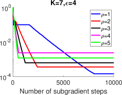
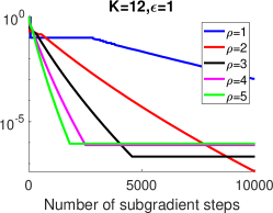
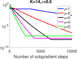
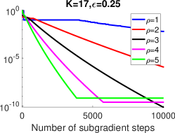
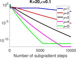
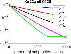
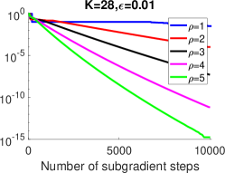
Figure 1: Performance of RLS on a simple linear program with $d=1$ and different values of $\rho$ and $\epsilon$.

5.2 Classification problem with fairness constraints.

Consider a set of $n$ data points $\mathcal{D}=\{({\mathbf{a}}_{i},b_{i})\}_{i=1}^{n}$ where ${\mathbf{a}}_{i}\in\mathbb{R}^{p}$ denotes a feature vector, and $b_{i}\in\{1,-1\}$ represents the class label for $i=1,2,\dots,n$. Let $\mathcal{D}_{M}\subset\mathbb{R}^{p}$ and $\mathcal{D}_{F}\subset\mathbb{R}^{p}$ be two different sensitive groups of instances. We want to find a linear classifier ${\mathbf{x}}\in\mathbb{R}^{p}$ that not only predicts the labels well (i.e., minimizes a loss function) but also treats each sensitive instance from $\mathcal{D}_{M}$ and $\mathcal{D}_{F}$ fairly. Such classification problems are suitable for applications such as loan approval or hiring decisions. For example, in the context of loan approval, we can ensure that loans are equally provided for different applicants independent of their group memberships (e.g., home-ownership or their gender). A correct classifier ${\mathbf{x}}$ satisfies $b_{i}{\mathbf{a}}_{i}^{\top}{\mathbf{x}}>0$ for all $i$. One can train such a classifier by solving the following optimization problems that minimizes a non-increasing convex loss function $\phi(\cdot)$ subject to fairness constraints:

$$\min_{{\mathbf{x}}} \frac{1}{n}\sum_{i=1}^{n}\phi(-b_{i}{\mathbf{a}}_{i}^{\top}{\mathbf{x}})$$ (40)

s.t. $$\frac{1}{n_{F}}\sum_{{\mathbf{a}}\in\mathcal{D}_{F}}\sigma({\mathbf{a}}^{\top}{\mathbf{x}})\geq\frac{\kappa}{n_{M}}\sum_{{\mathbf{a}}\in\mathcal{D}_{M}}\sigma({\mathbf{a}}^{\top}{\mathbf{x}}),$$ (42)

$$\frac{1}{n_{M}}\sum_{{\mathbf{a}}\in\mathcal{D}_{M}}\sigma({\mathbf{a}}^{\top}{\mathbf{x}})\geq\frac{\kappa}{n_{F}}\sum_{{\mathbf{a}}\in\mathcal{D}_{F}}\sigma({\mathbf{a}}^{\top}{\mathbf{x}}),$$

where $\kappa\in(0,1]$ is a constant, $n_{M}$ and $n_{F}$ are respectively the number of instances in $D_{M}$ and $D_{F}$, and finally $\sigma({\mathbf{a}}^{\top}{\mathbf{x}}):=\max\{0,\min\{1,\{0.5+{\mathbf{a}}^{\top}{\mathbf{x}}\}\}\in[0,1]$ is the probability of predicting ${\mathbf{a}}$ in class $+1$. The constraint (42) guarantees that the percentage of the instances in $\mathcal{D}_{F}$ that are predicted in class $+1$ is at least a $\kappa>0$ fraction of that in $\mathcal{D}_{M}$. The constraint (42) has a similar interpretation for instances in $\mathcal{D}_{M}$. Choosing an appropriate $\kappa$ ensures that the obtained classifier is fair to both $\mathcal{D}_{M}$ and $\mathcal{D}_{F}$ groups. An analogous model was considered in [13].

Constraints (42) and (42) are non-convex, so we approximate this problem by a convex optimization problem following the approach described in [24]. In particular, we reformulate the first constraint as

$$\frac{\kappa}{n_{M}}\sum_{{\mathbf{a}}\in\mathcal{D}_{M}}\sigma({\mathbf{a}}^{\top}{\mathbf{x}})+\frac{1}{n_{F}}\sum_{{\mathbf{a}}\in\mathcal{D}_{F}}\sigma(-{\mathbf{a}}^{\top}{\mathbf{x}})\leq 1$$

by using $\sigma({\mathbf{a}}^{\top}{\mathbf{x}})=1-\sigma(-{\mathbf{a}}^{\top}{\mathbf{x}})$. In addition, the function $\sigma({\mathbf{a}}^{\top}{\mathbf{x}})$ can be approximated by $(0.5+{\mathbf{a}}^{\top}{\mathbf{x}})_{+}=\max\{0,0.5+{\mathbf{a}}^{\top}{\mathbf{x}}\}$. Hence, we can rewrite the constraint (42) as a convex constraint:

$$\frac{\kappa}{n_{M}}\sum_{{\mathbf{a}}\in\mathcal{D}_{M}}({\mathbf{a}}^{\top}{\mathbf{x}}+0.5)_{+}+\frac{1}{n_{F}}\sum_{{\mathbf{a}}\in\mathcal{D}_{F}}(-{\mathbf{a}}^{\top}{\mathbf{x}}+0.5)_{+}\leq 1.$$

Applying a similar convex approximation to (42), we obtain the following convex reformulation of (40):

$$\min_{\|{\mathbf{x}}\|_{2}\leq\lambda} \frac{1}{n}\sum_{i=1}^{n}\phi(-b_{i}{\mathbf{a}}_{i}^{\top}{\mathbf{x}})$$ (43)

s.t. $$\frac{\kappa}{n_{M}}\sum_{{\mathbf{a}}\in\mathcal{D}_{M}}({\mathbf{a}}^{\top}{\mathbf{x}}+0.5)_{+}+\frac{1}{n_{F}}\sum_{{\mathbf{a}}\in\mathcal{D}_{F}}(-{\mathbf{a}}^{\top}{\mathbf{x}}+0.5)_{+}\leq 1,$$

$$\frac{\kappa}{n_{F}}\sum_{{\mathbf{a}}\in\mathcal{D}_{F}}({\mathbf{a}}^{\top}{\mathbf{x}}+0.5)_{+}+\frac{1}{n_{M}}\sum_{{\mathbf{a}}\in\mathcal{D}_{M}}(-{\mathbf{a}}^{\top}{\mathbf{x}}+0.5)_{+}\leq 1.$$

The above reformulation contains piece-wise linear functions (non-smooth) in its objective and constraints. Hence, this problem satisfies the error bound condition (2) with $d=1$ and an unknown value of $G$. We implemented RLS (Algorithm 2) to solve (43) using SGD in each $\mathtt{fom}_{k}$ instance to solve the subproblem $\min_{{\mathbf{x}}\in\mathcal{X}}P({\mathbf{x}}_{k},r_{k})$. We compare the performance of our method with three parameter-free but non-adaptive benchmarks: (1) the feasible level-set (FLS) method described in [23]; (2) the stochastic subgradient method by Yu, Neely, and Wei (YNW) in [47]; and (3) the switching gradient (SWG) method in [2] which is based on a mirror descent algorithm and a switching sub-gradient scheme . We choose these benchmarks as they are the most representative first-order methods that can solve “non-smooth” convex “constrained” optimization problems. The FLS is a level-set method guarantees the feasibility of the solutions generated at each iteration but does not exploit the error bound condition as our method does. Hence, it has a higher complexity bound for the class of problems that satisfy the error bound condition (2). YNW is a primal-dual method with dual variables updated implicitly while SWG is a pure primal method. We used the number of equivalent data passes performed by each algorithm as a measure of complexity.

Instances: To check the performance of the above mentioned methods, we considered three classification problems using (i) “LoanStats” data set from lending club which is a platform that allows individuals lend to other individuals; (ii) “COMPAS” data set from ProPublica; and (iii) “German” data set from UCI Machine Learning Repository.

The LoanStats data set contains information of $128,375$ loans issued on the loan club platform in the fourth quarter of 2018. The goal in this application is to predict whether a loan request will be approved or rejected. After creating dummy variables, each loan in this data set is represented by a vector of 250 features. We randomly partitioned this data set into a set of $63,890$ examples to construct the objective function and a set of $64,485$ examples to construct the constraints. The set $D_{M}$ in this application denotes the set of instances with “home-ownership = Mortgage”. All the other instances are considered in the set $D_{F}$. The fairness constraints in this application guarantees that customers with mortgage will not be disproportionally affected to receive new loans.

The COMPAS dataset includes the criminal history, jail and prison time, and demographics along with other factors of 6,172 instances. The goal of this application is to predict whether a person will be rearrested within two years after the first arrest. This information, for example, helps judges make bail decisions by predicting defendants’ criminal recidivism risk. We used $4,115$ of the examples in this dataset to formulate the objective function and the remaining to formulate the constraints. We chose sets $D_{M}$ and $D_{F}$ to respectively be the sets of male and female instances to ensure fair treatments among different genders.

The German credit dataset describes financial details of customers and is used to determine whether the customer should be granted credit (i.e. is a good customer) or not (i.e. is a bad customer). This dataset contains 1,000 instances and 50 variables. We used $667$ of the examples to formulate the objective function and the remaining to formulate the constraints. Similar to COMPAS data, the sets $D_{M}$ and $D_{F}$ respectively denote male and female examples.

In all above applications, we chose $\kappa=0.9$, and $\phi(z)=(1-z)_{+}$. We terminated RLS and other three benchmarks when the number of data passes reached 20,000. However, we ran the two level-set methods, i.e., RLS and FLS, longer for 100,000 data passes to find the optimal value $f^{*}$. In particular, we selected the smallest objective value among all $10^{-5}$-feasible solutions as a close approximation of $f^{*}$. We used this value to compute and plot $P(x;f^{*})$.

Algorithmic configurations: We next describe how we selected each of the parameters used in RLS, FLS, YNW, and SWG.

• RLS: We executed Algorithm 2 on all of our instances with $\epsilon=0.001$. We used cross-validation to chose a value for $\alpha$ from $\{0.3,0.5,0.9\}$ and for $B$ from $\{0.9,0.95,0.99\}$ to minimize the value of $P({\mathbf{x}};f^{*})$ at termination. Since the optimal value of (43) is positive, we set $r_{\text{ini}}=0$ to satisfy the condition $r_{\text{ini}}<f^{*}$. Although the vector of all zeros could be used as an initial solution ${\mathbf{x}}_{\text{ini}}$, we used a different value in our algorithm. In particular, the complexity bound of RLS shows that the algorithm requires less number of iterations if $g({\mathbf{x}}_{\text{ini}})<0$ and is as small as possible. Hence, we followed a heuristic to obtain a better quality solution. We applied the SGD algorithm to minimize the function $g({\mathbf{x}})$ and used the returned solution after 40 iterations. Finding such solution accounted for less than 1% of our total-run time. Finally, we used $K=\tilde{K}$ where $\tilde{K}$ is computed according to the bound (11) for $r=r_{\text{ini}}$.

• FLS: The FLS algorithm described in [23] requires two input parameters: $r_{\text{ini}}>f^{*}$ and $\alpha>1$. To obtain $r_{\text{ini}}>f^{*}$, we first followed the same step as in RLS to obtain a feasible solution ${\mathbf{x}}_{\text{ini}}$ such that $g({\mathbf{x}}_{\text{ini}})<0$ and then set $r_{\text{ini}}=f({\mathbf{x}}_{\text{ini}})$. Since ${\mathbf{x}}_{\text{ini}}$ is feasible, using Lemma 2.1 we can guarantee that $r_{\text{ini}}>f^{*}$. We chose $\alpha$ from $\{100,200,500\}$ that produces the smallest $P({\mathbf{x}};f^{*})$ at termination.

• YNW: We followed the guidance in [47] to setup YNW. Specifically, we chose the control parameters $V$ and $\alpha$ as $V=\sqrt{T}$ and $\alpha=T$, respectively, as a function of the total number of iterations $T$, where $V$ is the weight of the gradient of the objective function and $\alpha$ is the weight of the proximal term in the updating equation of ${\mathbf{x}}$ in YNW. We chose the number of iterations $T$ such that its total data passes is $20,000$. We used the all-zero vector as an initial solution to YNW. Of course, for a fair comparison, the number of data passes that RLS and FLS spend in searching the initial solution is included when comparing the performances of these algorithms.

• SWG: The only input of SWG algorithm is the precision $\epsilon$. We selected $\epsilon$ from $\{0.01,0.001,0.0001\}$ to minimize the value of $P(x;f^{*})$ achieved by SWG at termination. It turned out $\epsilon=0.001$ gave the best performance for all the three datasets.

	LoanStats	COMPAS	German
$P({\mathbf{x}};f^{*})$
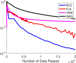
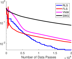
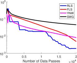
$f(x)-f^{*}$
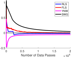
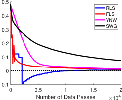
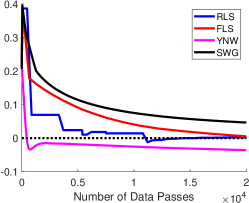
$\max\limits_{i=1,2,\dots,m}\{f_{i}({\mathbf{x}})\}$

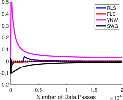
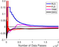
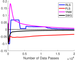
Figure 2: Performance of RLS, FLS, YNW, and SWG for solving binary classification problems with fairness constraints.

Results: Figure 2 displays the performance of RLS, FLS, YNW and SWG as a function of data passes. In particular, the $x$-axis in this figure shows the number of data passes each algorithm performed while the $y$-axis represents the feasibility and optimality of solutions returned by each method. More specifically, the $y$-axis in the first row of this plot represents $P({\mathbf{x}};f^{*})$. As explained before, this quantity is zero when the solution ${\mathbf{x}}$ is both feasible and optimal and positive otherwise. The speed at which $P({\mathbf{x}};f^{*})$ converges to zero indicates how fast the solution ${\mathbf{x}}$ becomes feasible and optimal at each iteration. The $y$-axis in the second row represents $f({\mathbf{x}})-f^{*}$ that measures the optimality gap at ${\mathbf{x}}$ and in the third row, $g({\mathbf{x}})=\max_{i=1,\ldots,m}\{f_{i}({\mathbf{x}})\}$ checks whether the solution ${\mathbf{x}}$ is feasible or not (if $g({\mathbf{x}})<0$ then ${\mathbf{x}}$ is feasible).

We observe that RLS achieves the fastest reduction in the function $P({\mathbf{x}};f^{*})$ on the three datasets. YNW has high constraints violation on LoanStats and German datasets. FLS and SWG are the only algorithms that maintain feasibility at each iteration and FLS reduces the optimaltiy gap faster than SWG. RLS achieves a good quality solution faster than FLS. Our computational results reveal that our algorithm compares favorable with other existing approaches in the literature.

6 Conclusion.

We develop an adaptive level-set method that is both parameter-free and projection-free for constrained convex optimization, that is, it accelerates under the error bound condition and does not require knowledge of unknown parameters or challenging projections for its execution. This method finds an $\epsilon$-optimal and $\epsilon$-feasible solution by considering a sequence of level-set subproblems that are solved in parallel using standard subgradient oracles with simple updates. These oracles restart based on objective function progress and communicate information between them upon each restart. We show that the iteration complexity of our restarting level set method is only worse by a log-factor in both the smooth and non-smooth settings compared to existing accelerated methods for constrained convex optimization under the error bound condition, all of which rely on either unknown parameters or sophisticated oracles (e.g., involving difficult projection or exact line search). Numerical experiments show that the proposed method exhibits promising performance relative to benchmarks on a constrained classification problem.

This section contains the proof of Lemma 3.8 and presents Lemma 6.7 and Lemma 6.9 that formally prove the inequalities (20) and (21) used in the proof of Theorem 3.9. For all the results included in this section, we need to introduce slightly different notations representing ${\mathbf{x}}_{k}^{(t_{k})}$ and $r_{k}$ to account for the number of restarts in each $\mathtt{fom}$ instance. More precisely, we use the notation ${\mathbf{x}}_{k}^{(l_{k},t_{k})}$ and $r_{k}^{(l_{k})}$ to respectively represent the solution in the $t_{k}$th iteration of $\mathtt{fom}_{k}$ after $l_{k}$ restarts and the level parameter in $\mathtt{fom}_{k}$ after $l_{k}$ restarts.

In the proof of the lemmas below we require the result of propositions 6.1 and 6.3.

Proposition 6.1

The function $P({\mathbf{x}},r)+r$ is an increasing function in $r$ for any ${\mathbf{x}}\in\mathcal{X}$.

Proof 6.2

Proof. The proof of this proposition follows from the convexity of $P({\mathbf{x}};r)$ in $r$. In particular, let $\xi_{r}$ denote the sub-gradient of $P(\cdot;r)$ with respect to $r$. It is straightforward to see $\xi_{r}\in[-1,0]$ for any $r$. Hence, from convexity of $P({\mathbf{x}};r)$ in $r$, it follows that for $r\geq r^{\prime}$, we have $P({\mathbf{x}};r)\geq P({\mathbf{x}};r^{\prime})+\xi_{r}(r-r^{\prime})\geq P({\mathbf{x}};r^{\prime})-1\cdot(r-r^{\prime})$ which indicates $P({\mathbf{x}};r)+r\geq P({\mathbf{x}};r^{\prime})+r^{\prime}.$

Proposition 6.3

Consider $\alpha\in(0,1)$, $r_{\text{ini}}<f^{*}$, and a strictly feasible solution ${\mathbf{x}}_{\text{ini}}\in\mathcal{X}$ used in Algorithm 2. Suppose $k^{*}$ is a critical index. For any $l\geq 0$, we have

$$P({\mathbf{x}}_{k^{*}}^{(l,0)};r_{k^{*}}^{(l)})\leq f({\mathbf{x}}_{\text{ini}})-r_{\text{ini}}.$$ (44)

Proof 6.4

Proof The proof of this proposition relies on the fact that the function $P({\mathbf{x}}_{k^{*}}^{(l,0)};r_{k^{*}}^{(l)})+r_{k^{*}}^{(l)}$ is non-increasing in $l$. The value of this function does not change if the restart is not desirable since ${\mathbf{x}}_{k^{*}}^{(l,0)}$ and $r_{k^{*}}^{(l)}$ remain unchanged. It is easy to see that after each desirable restart, when $l$ increases, either $P(x_{k^{*}}^{(l,0)};\cdot)$ or $r_{k^{*}}^{(l)}$ decreases. In both cases, the function $P({\mathbf{x}}_{k^{*}}^{(l,0)};r_{k^{*}}^{(l)})+r_{k}^{(l)}$ reduces (see (10) and Proposition 6.1). Therefore, we can write

$$P({\mathbf{x}}_{k^{*}}^{(l,0)};r_{k^{*}}^{(l)})+r_{k^{*}}^{(l)}\leq P({\mathbf{x}}_{k^{*}}^{(0,0)};r_{k^{*}}^{(0)})+r_{k^{*}}^{(0)}=P({\mathbf{x}}_{\text{ini}};r_{k^{*}}^{(0)})+r_{k^{*}}^{(0)}.$$

We claim $r_{k^{*}}^{(0)}\leq f({\mathbf{x}}_{\text{ini}})$. Assuming this claim is true, using the above inequality, Proposition 6.1, and the fact that $P({\mathbf{x}}_{\text{ini}};f({\mathbf{x}}_{\text{ini}}))=0$, we obtain

$$P({\mathbf{x}}_{k^{*}}^{(l,0)};r_{k^{*}}^{(l)})+r_{k^{*}}^{(l)}\leq P({\mathbf{x}}_{\text{ini}};f({\mathbf{x}}_{\text{ini}}))+f({\mathbf{x}}_{\text{ini}})=f({\mathbf{x}}_{\text{ini}}).$$

In addition, since $r_{\text{ini}}=r_{0}^{(l)}<r_{k^{*}}^{(l)}$ we obtain $P({\mathbf{x}}_{k^{*}}^{(l,0)};r_{k^{*}}^{(l)})\leq f({\mathbf{x}}_{\text{ini}})-r_{k^{*}}^{(l)}\leq f({\mathbf{x}}_{\text{ini}})-r_{\text{ini}}$. The equation $r_{\text{ini}}=r_{0}^{(l)}$ holds since $r_{0}$ initiated at $r_{\text{ini}}$ does not change throughout the algorithm and the inequality $r_{0}^{(l)}<r_{k^{*}}^{(l)}$ follows from Theorem 3.4. To complete the proof, we need to show our claim is true. We actually show that this claim holds at any index $k$. Since ${\mathbf{x}}_{\text{ini}}$ is a strictly feasible solution, it is straightforward to see $r_{0}^{(0)}\leq f^{*}<f({\mathbf{x}}_{\text{ini}})$ and $P({\mathbf{x}}_{\text{ini}};r_{k}^{(0)})=f({\mathbf{x}}_{\text{ini}})-r_{k}^{(0)}$ for all $k$. Given $k\geq 0$, it follows from this equality and the updates of level parameters that $r_{k}^{(0)}$ can be written as a convex combination of $r_{k-1}^{(0)}$ and $f({\mathbf{x}}_{\text{ini}})$. In particular, $r_{k}^{(0)}=r_{k-1}^{(0)}+\alpha P({\mathbf{x}}_{k-1}^{(0,0)};r_{k-1}^{(0)})=r_{k-1}^{(0)}+\alpha P({\mathbf{x}}_{\text{ini}};r_{k-1}^{(0)})=r_{k-1}^{(0)}+\alpha(f({\mathbf{x}}_{\text{ini}})-r_{k-1}^{(0)})=(1-\alpha)r_{k-1}^{(0)}+\alpha f({\mathbf{x}}_{\text{ini}})$. Our claim will then follow by applying this equation recursively since $r_{0}^{(0)}<f({\mathbf{x}}_{\text{ini}})$.

Let $k^{\prime}$ be the smallest index at which the inequalities $P({\mathbf{x}}_{k^{\prime}}^{(l_{k^{\prime}},t_{k^{\prime}})};r_{k^{\prime}}^{(l_{k^{\prime}})})\leq BP({\mathbf{x}}_{k^{\prime}}^{(l_{k^{\prime}},0)};r_{k^{\prime}}^{(l_{k^{\prime}})})$ and $P({\mathbf{x}}_{k^{\prime}}^{(l_{k^{\prime}},0)};r_{k^{\prime}}^{(l_{k^{\prime}})})\geq 0$ hold (i.e. $k^{\prime}$ is the index found in Line 7 of Algorithm 2). RLS then initiates a restart at this index and also restarts all instances whose indices are greater than $k^{\prime}$. Suppose this is the $l_{k}$th restart at $\mathtt{fom}_{k}$ for $k\geq k^{\prime}$. To understand how level parameters change after each restart, we reply on the following lemma where we provide a lower bound on $r_{k}^{(l_{k}-1)}-r_{k}^{(l_{k})}$ for each $k\geq k^{\prime}$.

Lemma 6.5

Suppose $\alpha$ and $B$ are such that $0<\alpha<B<1$. Let $k^{\prime}$ be the index found in Line 7 of Algorithm 2. In addition, assume the level parameters $r_{k}^{(l_{k})}$ for $k\geq k^{\prime}$ are updated as in Line 11, i.e., $r_{k}^{(l_{k})}=r_{k-1}^{(l_{k-1})}+\alpha P({\mathbf{x}}_{k-1}^{(l_{k-1},0)};r_{k-1}^{(l_{k-1})})$ for $k\geq k^{\prime}+1$. We then have

$$r_{k^{\prime}}^{(l_{k^{\prime}}-1)}-r_{k^{\prime}}^{(l_{k^{\prime}})}=0,$$ (45)

and

$$r_{k}^{(l_{k}-1)}-r_{k}^{(l_{k})}\geq(1-\alpha)^{k-k^{\prime}-1}\alpha(1-B)P({\mathbf{x}}_{k^{\prime}}^{(l_{k^{\prime}}-1,0)};r_{k^{\prime}}^{(l_{k^{\prime}}-1)})\quad\text{for }k\geq k^{\prime}+1.$$ (46)

Proof 6.6

Proof. The equation $r_{k^{\prime}}^{(l_{k^{\prime}})}=r_{k^{\prime}}^{(l_{k^{\prime}}-1)}$ directly follows from the steps of Algorithm 2. In particular, the level parameters are only updated for $k\geq k^{\prime}+1$ after each restart at index $k^{\prime}$. Recall that the index $k^{\prime}$ is selected such that $P({\mathbf{x}}_{k^{\prime}}^{(l_{k^{\prime}}-1,0)};r_{k^{\prime}}^{(l_{k^{\prime}}-1)})\geq 0$ and $P({\mathbf{x}}_{k^{\prime}}^{(l_{k^{\prime}}-1,t_{k^{\prime}})};r_{k^{\prime}}^{(l_{k^{\prime}}-1)})\leq BP({\mathbf{x}}_{k^{\prime}}^{(l_{k^{\prime}}-1,0)};r_{k^{\prime}}^{(l_{k^{\prime}}-1)}).$ Since ${\mathbf{x}}_{k^{\prime}}^{(l_{k^{\prime}},0)}={\mathbf{x}}_{k^{\prime}}^{(l_{k^{\prime}}-1,t_{k^{\prime}})}$ and $r_{k^{\prime}}^{(l_{k^{\prime}})}=r_{k^{\prime}}^{(l_{k^{\prime}}-1)}$, we get

$$P({\mathbf{x}}_{k^{\prime}}^{(l_{k^{\prime}},0)};r_{k^{\prime}}^{(l_{k^{\prime}})})\leq BP({\mathbf{x}}_{k^{\prime}}^{(l_{k^{\prime}}-1,0)};r_{k^{\prime}}^{(l_{k^{\prime}}-1)}).$$ (47)

Now let’s consider the index $k^{\prime}+1$:

$$r_{k^{\prime}+1}^{(l_{k^{\prime}+1}-1)}-r_{k^{\prime}+1}^{(l_{k^{\prime}+1})} = r_{k^{\prime}}^{(l_{k^{\prime}}-1)}+\alpha P({\mathbf{x}}_{k^{\prime}}^{(l_{k^{\prime}}-1,0)};r_{k^{\prime}}^{(l_{k^{\prime}}-1)})-r_{k^{\prime}}^{(l_{k^{\prime}})}-\alpha P({\mathbf{x}}_{k^{\prime}}^{(l_{k^{\prime}},0)};r_{k^{\prime}}^{(l_{k^{\prime}})})$$ (48)

$$= \alpha P({\mathbf{x}}_{k^{\prime}}^{(l_{k^{\prime}}-1,0)};r_{k^{\prime}}^{(l_{k^{\prime}}-1)})-\alpha P({\mathbf{x}}_{k^{\prime}}^{(l_{k^{\prime}},0)};r_{k^{\prime}}^{(l_{k^{\prime}})})$$

$$\geq \alpha P({\mathbf{x}}_{k^{\prime}}^{(l_{k^{\prime}}-1,0)};r_{k^{\prime}}^{(l_{k^{\prime}}-1)})-\alpha BP({\mathbf{x}}_{k^{\prime}}^{(l_{k^{\prime}}-1,0)};r_{k^{\prime}}^{(l_{k^{\prime}}-1)})$$

$$= \alpha(1-B)P({\mathbf{x}}_{k^{\prime}}^{(l_{k^{\prime}}-1,0)};r_{k^{\prime}}^{(l_{k^{\prime}}-1)}),$$

where we used the definitions of $r_{k^{\prime}+1}$ to obtain the first equality; (45) for the second; and (47) for the first inequality; Similarly for $k\geq k^{\prime}+2$, we show

$$r_{k}^{(l_{k}-1)}-r_{k}^{(l_{k})} = r_{k-1}^{(l_{k-1}-1)}+\alpha P({\mathbf{x}}_{k-1}^{(l_{k-1}-1,0)};r_{k-1}^{(l_{k-1}-1)})-r_{k-1}^{(l_{k-1})}-\alpha P({\mathbf{x}}_{k-1}^{(l_{k-1},0)};r_{k-1}^{(l_{k-1})})$$ (49)

$$= r_{k-1}^{(l_{k-1}-1)}-r_{k-1}^{(l_{k-1})}+\alpha P({\mathbf{x}}_{k-1}^{(l_{k-1},0)};r_{k-1}^{(l_{k-1}-1)})-\alpha P({\mathbf{x}}_{k-1}^{(l_{k-1},0)};r_{k-1}^{(l_{k-1})})$$

$$\geq (1-\alpha)(r_{k-1}^{(l_{k-1}-1)}-r_{k-1}^{(l_{k-1})}),$$

where the second equality follows from ${\mathbf{x}}_{k-1}^{(l_{k-1},0)}={\mathbf{x}}_{k-1}^{(l_{k-1}-1,0)}$ and the last inequality form Proposition 6.1 and the fact that $r_{k-1}^{(l_{k-1}-1)}\geq r_{k-1}^{(l_{k-1})}$ for $k\geq k^{\prime}+2$ which can be easily verified by combining (48) and (49) and the inequality $P({\mathbf{x}}_{k^{\prime}}^{(l_{k^{\prime}}-1,0)};r_{k^{\prime}}^{(l_{k^{\prime}}-1)})\geq 0$. Applying (49) recursively along with (48) proves (46).

Proof of Lemma 3.8: To prove this lemma, we claim that if the inequality (5) ($\alpha P({\mathbf{x}}_{k}^{(0)};r_{k})\leq f^{*}-r_{k}$) is satisfied at some $k$, it will continue to be satisfied after each restart. By Theorem 3.4, it will then follows that none of the indices that are smaller than the current critical index can become a critical index after the restarts. Therefore, the critical index cannot decrease throughout the algorithm. Our claim can be proved by defining the quantity $V_{k}\left(l_{k}\right)$, $k=0,1,2,\ldots$ as follows:

$$V_{k}\left(l_{k}\right):=f^{*}-r_{k}^{(l_{k})}-\alpha P({\mathbf{x}}_{k}^{(l_{k},0)};r_{k}^{(l_{k})}).$$ (50)

We show $V_{k}(l_{k})$ is a non-decreasing function of $l_{k}$ when the inequality (5) holds at index $k$. More precisely, we show the inequality $V_{k}(l_{k})\geq V_{k}(l_{k}-1)$ holds for such $k$. Therefore, assuming (5) is satisfied in $l_{k}-1$ restarts, it will continue to hold after next restart since $V_{k}(l_{k})\geq V_{k}(l_{k}-1)\geq 0$.

Fix an index $k\in[0,\tilde{K}]$ for which we have $\alpha P({\mathbf{x}}_{k}^{(l_{k}-1,0)};r_{k}^{(l_{k}-1)})<f^{*}-r_{k}^{(l_{k}-1)}$. The restarts that occur at larger indices than $k$ do not change $V_{k}(l_{k}-1)$ since ${\mathbf{x}}_{k}^{(l_{k}-1,0)}$ and $r_{k}^{(l_{k}-1)}$ remain the same. Therefore, we only focus on the restarts that either happen (i) at index $k$ or (ii) any smaller index than $k$.

Case (i): When the restart occurs at index $k$, it means we have found a solution ${\mathbf{x}}_{k}^{(l_{k}-1,t_{k})}$ such that $P({\mathbf{x}}_{k}^{(l_{k}-1,0)};r_{k}^{(l_{k}-1)})\geq 0$ and

$$P({\mathbf{x}}_{k}^{(l_{k}-1,t_{k})};r_{k}^{(l_{k}-1)})\leq BP({\mathbf{x}}_{k}^{(l_{k}-1,0)};r_{k}^{(l_{k}-1)}).$$

Since ${\mathbf{x}}_{k}^{(l_{k},0)}={\mathbf{x}}_{k}^{(l_{k}-1,t_{k})}$ and $r_{k}^{(l_{k})}=r_{k}^{(l_{k}-1)}$ which follows from the restarting steps, we get

$$P({\mathbf{x}}_{k}^{(l_{k},0)};r_{k}^{(l_{k})})\leq BP({\mathbf{x}}_{k}^{(l_{k}-1,0)};r_{k}^{(l_{k}-1)}).$$

Using this inequality and the fact that $r_{k}^{(l_{k})}=r_{k}^{(l_{k}-1)}$, it is straightforward to see $V_{k}(l_{k})\geq V_{k}(l_{k}-1)+\alpha(1-B)P({\mathbf{x}}_{k}^{(l_{k}-1,0)};r_{k}^{(l_{k}-1)})$. This inequality further implies that

$$V_{k}(l_{k}) \geq V_{k}(l_{k}-1)+\alpha(1-B)P({\mathbf{x}}_{k}^{(l_{k}-1,0)};r_{k}^{(l_{k}-1)})$$

$$\geq V_{k}(l_{k}-1)+\alpha(1-B)\theta\left(f^{*}-r_{k}^{(l_{k}-1)}\right)$$

$$>V_{k}(l_{k}-1)+\alpha(1-B)\theta(f^{*}-r_{k}^{(l_{k}-1)}-\alpha P({\mathbf{x}}_{k}^{(l_{k}-1,0)};r_{k}^{(l_{k}-1)}))$$

$$=\left(1+\alpha(1-B)\theta\right)V_{k}(l_{k}-1),$$

$$>V_{k}(l_{k}-1)$$ (51)

where the second inequality follows from $0\leq\alpha P({\mathbf{x}}_{k}^{(l_{k}-1,0)};r_{k}^{(l_{k}-1)})\leq f^{*}-r_{k}^{(l_{k}-1)}$ and Lemma 2.3 that shows $\theta\leq\frac{H(r_{k}^{(l_{k}-1)})}{f^{*}-r_{k}^{(l_{k}-1)}}\leq\frac{P({\mathbf{x}}_{k}^{(l_{k}-1,0)};r_{k}^{(l_{k}-1)})}{f^{*}-r_{k}^{(l_{k}-1)}}$, and the third from the inequality $P({\mathbf{x}}_{k}^{(l_{k}-1,0)};r_{k}^{(l_{k}-1)})\geq 0$ which holds since the restart has occurred at index $k$.

Case (ii): In this case we have ${\mathbf{x}}_{k}^{(l_{k},0)}={\mathbf{x}}_{k}^{(l_{k}-1,0)}$ and $r_{k}^{(l_{k}-1)}\geq r_{k}^{(l_{k})}$ which follow from the restarting steps and Lemma 6.5. Hence,

$$V_{k}(l_{k})=f^{*}-r_{k}^{(l_{k})}-\alpha P({\mathbf{x}}_{k}^{(l_{k},0)};r_{k}^{(l_{k})})\geq f^{*}-r_{k}^{(l_{k}-1)}-\alpha P({\mathbf{x}}_{k}^{(l_{k}-1,0)};r_{k}^{(l_{k}-1)})=V_{k}(l_{k}-1),$$ (52)

where the inequality follows from the fact that the function $f^{*}-r-\alpha P({\mathbf{x}};r)$ is decreasing in $r$ for any ${\mathbf{x}}\in\mathcal{X}$ (see Proposition 6.1). Considering (51) and (52), our proof is complete.

In the following lemmas we prove the inequalities (20) and (21) used in the proof of Theorem 3.9 in Section 3.

Lemma 6.7

Suppose $\alpha$, $B$, and $\epsilon$ are such that $0<\alpha<B<1$ and $\epsilon>0$. Consider an index $k$ and $\tilde{K}$ as defined in (11) for $r=r_{\text{ini}}$. Let $D_{k}$ denote the total number of desirable restarts starting at $\mathtt{fom}_{k}$ until an $\epsilon$-optimal and $\epsilon$-feasible solution in found. Then we have

$$D_{k}=\sum_{k^{*}=k+1}^{\tilde{K}}D_{kk^{*}}\leq\ln\left(\dfrac{2(f^{*}-r_{\text{ini}})}{\alpha\epsilon}\right)/\ln\left(1+\alpha(1-B)\theta/2\right),$$

where $D_{kk^{*}}$ is the total number of desirable restarts starting at $\mathtt{fom}_{k}$ with $k<k^{*}$ assuming $k^{*}$ is the critical index at the time of restart.

Proof 6.8

Proof. Using the definitions of $D_{k}$ and $D_{kk^{*}}$, it is easy to see that $D_{k}=\sum_{k^{*}=k+1}^{\tilde{K}}D_{kk^{*}}$ because by Lemma 3.8, the critical index $k^{*}$ is non-decreasing and can vary between $k+1$ and $\tilde{K}$. Let’s consider a modification of the quantity $V_{k}(l_{k})$ defined in (50). In other words, we define

$$V^{\prime}_{k}(l_{k}):=f^{*}-r_{k}^{(l_{k})}-\dfrac{\alpha}{2}P({\mathbf{x}}_{k}^{(l_{k},0)};r_{k}^{(l_{k})}).$$

Since $k$ is smaller index than a critical index, using Theorem 3.4, for all $l_{k}\geq 0$ we can verify that $V^{\prime}_{k}(l_{k})>0$, $r_{k}^{(l_{k})}<f^{*}$ and hence $P({\mathbf{x}}_{k}^{(l_{k},0)};r_{k}^{(l_{k})})\geq H(r_{k}^{(l_{k})})>0$ , and $r_{k}^{(l_{k})}\geq r_{0}^{(l_{0})}$. In addition, Theorem 3.4 also indicates that the inequality (5) holds at $k$. Hence, following the same proof as in the proof of Lemma 3.8, one can show

$$V^{\prime}_{k}(l_{k})\geq\left(1+\alpha(1-B)\theta/2\right)V^{\prime}_{k}(l_{k}-1),$$

if the restarts occurs at index $k$ and

$$V^{\prime}_{k}(l_{k})\geq V^{\prime}_{k}(l_{k}-1),$$

if the restarts occurs at an index smaller than $k$. Suppose $\hat{l}_{k}$ denotes the smallest restarting iteration at which the index $k$ becomes smaller than a critical index. By recursively applying the above inequality, we obtain

$$V^{\prime}_{k}(l_{k}) \geq\left(1+\alpha(1-B)\theta/2\right)^{D_{k}}V^{\prime}_{k}(\hat{l}_{k})$$

$$=\left(1+\alpha(1-B)\theta/2\right)^{D_{k}}\left(f^{*}-r_{k}^{(\hat{l}_{k})}-\dfrac{\alpha}{2}P({\mathbf{x}}_{k}^{(\hat{l}_{k},0)};r_{k}^{(\hat{l}_{k})})\right).$$ (53)

Given that $k$ is smaller than a critical index, following Theorem 3.4 we have $0<\alpha P({\mathbf{x}}_{k}^{(\hat{l}_{k},0)};r_{k}^{(\hat{l}_{k})})<f^{*}-r_{k}^{(\hat{l}_{k})}$ which implies

$$f^{*}-r_{k}^{(\hat{l}_{k})}-\dfrac{\alpha}{2}P({\mathbf{x}}_{k}^{(\hat{l}_{k},0)};r_{k}^{(\hat{l}_{k})})>\dfrac{\alpha}{2}P({\mathbf{x}}_{k}^{(\hat{l}_{k},0)};r_{k}^{(\hat{l}_{k})})>\dfrac{\alpha\epsilon}{2},$$ (54)

where the last inequality follows from the fact that $r_{k}^{(\hat{l}_{k})}<f^{*}$ and ${\mathbf{x}}_{k}^{(\hat{l}_{k},0)}$ is not $\epsilon$-feasible and $\epsilon$-optimal (see Lemma 2.2). On the other hand, since $P({\mathbf{x}}_{k}^{(l_{k},0)};r_{k}^{(l_{k})})\geq H(r_{k}^{(l_{k})})>0$ and $r_{0}=r_{\text{ini}}$ remains the same throughout the Algorithm 2, we also get

$$V^{\prime}_{k}(l_{k})<f^{*}-r_{k}^{(l_{k})}\leq f^{*}-r_{0}^{(l_{k})}=f^{*}-r_{\text{ini}}.$$ (55)

It follows from (53), (54), and (55) that

$$\left(1+\alpha(1-B)\theta/2\right)^{D_{k}}\dfrac{\alpha\epsilon}{2}\leq f^{*}-r_{\text{ini}}.$$

We can then obtain our desirable bound on $D_{k}$ by taking a logarithmic transformation on both sides of the above inequality and organizing terms.

Lemma 6.9

Suppose $\alpha$, $B$, and $\epsilon$ are such that $0<\alpha<B<1$ and $\epsilon>0$. Consider a critical index $k^{*}$ and $\tilde{K}$ as defined in (11) for $r=r_{\text{ini}}$. Let $D_{k^{*}k^{*}}$ denote the total number of desirable restarts starting at $\mathtt{fom}_{k^{*}}$ before the critical index increases or an $\epsilon$-feasible and $\epsilon$-optimal solution is found. Then

$$D_{k^{*}k^{*}}\leq\left[\tilde{K}\ln\left(\dfrac{1}{1-\alpha}\right)+\ln\left(\frac{f^{*}-r_{\text{ini}}}{\alpha(1-B)\epsilon}\right)+2\ln\left(\dfrac{f({\mathbf{x}}_{\text{ini}})-r_{\text{ini}}}{\epsilon}\right)\right]/\ln(1/B).$$

Proof 6.10

Proof. Suppose $k^{*}$ is the critical index between iterations $T_{0}$ and $T_{1}$ while there is no $\epsilon$-feasible and $\epsilon$-optimal solution is found in between (i.e. the critical index increases at iterations $T_{1}$). To bound $D_{k^{*}k^{*}}$, let’s consider two cases:

Case $i$: All desirable restarts between $T_{0}$ and $T_{1}$ are from $\mathtt{fom}_{k^{*}}$: Recall that the $l_{k^{*}}$th restart happens when a solution ${\mathbf{x}}_{k^{*}}^{(l_{k^{*}}-1,t_{k^{*}})}$ is found such that $P({\mathbf{x}}_{k^{*}}^{(l_{k^{*}}-1,0)};r_{k^{*}}^{(l_{k^{*}}-1)})\geq 0$ and

$$P({\mathbf{x}}_{k^{*}}^{(l_{k^{*}}-1,t_{k^{*}})};r_{k^{*}}^{(l_{k^{*}}-1)})\leq BP({\mathbf{x}}_{k^{*}}^{(l_{k^{*}}-1,0)};r_{k^{*}}^{(l_{k^{*}}-1)}).$$

Since ${\mathbf{x}}_{k^{*}}^{(l_{k^{*}},0)}={\mathbf{x}}_{k^{*}}^{(l_{k^{*}}-1,t_{k^{*}})}$ and $r_{k^{*}}^{(l_{k^{*}})}=r_{k^{*}}^{(l_{k^{*}}-1)}$, the above inequality indicates that the function $P({\mathbf{x}}_{k^{*}}^{(l_{k^{*}},0)};r_{k^{*}}^{(l_{k^{*}})})$ reduces by a factor of $B$ at each desirable restart since

$$P({\mathbf{x}}_{k^{*}}^{(l_{k^{*}},0)};r_{k^{*}}^{(l_{k^{*}})})\leq BP({\mathbf{x}}_{k^{*}}^{(l_{k^{*}}-1,0)};r_{k^{*}}^{(l_{k^{*}}-1)}).$$

In addition, since there is no $\epsilon$-feasible and $\epsilon$-optimal solution is found between $T_{0}$ and $T_{1}$, by Lemma 2.2 we must have $\epsilon<P({\mathbf{x}}_{k^{*}}^{(l_{k^{*}},0)};r_{k^{*}}^{(l_{k^{*}})})$ for any $l_{k^{*}}$. Let $\hat{l}_{k^{*}}<l_{k^{*}}$ denote the restarting iteration at which $k^{*}$ becomes a critical index. The above arguments, therefore, imply

$$\epsilon\leq B^{D_{k^{*}k^{*}}}P({\mathbf{x}}_{k^{*}}^{(\hat{l}_{k^{*}},0)};r_{k^{*}}^{(\hat{l}_{k^{*}})}).$$ (56)

We also know $0\leq P({\mathbf{x}}_{k^{*}}^{(\hat{l}_{k^{*}},0)};r_{k^{*}}^{(\hat{l}_{k^{*}})})\leq f({\mathbf{x}}_{\text{ini}})-r_{\text{ini}}$, where the first inequality follows from the fact that $r_{k^{*}}^{(\hat{l}_{k^{*}})}\leq f^{*}$ and the second from (44). Applying this inequality to (56) we obtain $\epsilon\leq B^{D_{k^{*}k^{*}}}(f({\mathbf{x}}_{\text{ini}})-r_{\text{ini}})$ which results in finding an upper bound for $D_{k^{*}k^{*}}$. i.e.,

$$D_{k^{*}k^{*}}\leq\ln\left(\frac{f({\mathbf{x}}_{\text{ini}})-r_{\text{ini}}}{\epsilon}\right)/\ln(1/B).$$

Case $ii$: At least one desirable restart between $T_{0}$ and $T_{1}$ happens at $\mathtt{fom}_{k}$ for some $k<k^{*}$: Suppose, the first desirable restart from $\mathtt{fom}_{k}$ happens at iteration $T_{0.5}$ with $T_{0}<T_{0.5}<T_{1}$. This means that all desirable restarts between $T_{0}$ and $T_{0.5}$ are from $\mathtt{fom}_{k^{*}}$. Suppose $D_{k^{*}k^{*}}^{0}$ and $D_{k^{*}k^{*}}^{1}$ respectively denote the number of desirable restarts from $\mathtt{fom}_{k^{*}}$ between $T_{0}$ and $T_{0.5}$ and between $T_{0.5}$ and $T_{1}$. Following the analysis of Case $i$, one can show

$$D_{k^{*}k^{*}}^{0}\leq\ln\left(\frac{f({\mathbf{x}}_{\text{ini}})-r_{\text{ini}}}{\epsilon}\right)/\ln(1/B).$$

It only remains to find an upper bound for $D_{k^{*}k^{*}}^{1}$. Suppose, after the desirable restart at $T_{0.5}$, the solutions and the level parameters in $\mathtt{fom}_{k}$ and $\mathtt{fom}_{k^{*}}$ are $({\mathbf{x}}_{k}^{(l_{k},0)},r_{k}^{(l_{k})})$ and $({\mathbf{x}}_{k^{*}}^{(l_{k^{*}},0)},r_{k^{*}}^{(l_{k^{*}})})$, respectively. We have

$$f^{*}-r_{k^{*}}^{(l_{k^{*}})} >r_{k^{*}}^{(l_{k^{*}}-1)}-r_{k^{*}}^{(l_{k^{*}})}\geq(1-\alpha)^{k^{*}-k-1}\alpha(1-B)P({\mathbf{x}}_{k}^{(l_{k}-1,0)};r_{k}^{(l_{k}-1)})$$

$$>(1-\alpha)^{k^{*}-k-1}\alpha(1-B)\epsilon\geq(1-\alpha)^{\tilde{K}}\alpha(1-B)\epsilon,$$ (57)

where the first inequality follows from $r_{k^{*}}^{(l_{k^{*}}-1)}<f^{*}$ (see Theorem 3.4), the second from Lemma 6.5, and the third from the fact that ${\mathbf{x}}_{k}^{(l_{k}-1,0)}$ is not $\epsilon$-optimal and $\epsilon$-feasible. The last inequality holds since the critical index $k^{*}$ is no more than $\tilde{K}$ before an $\epsilon$-optimal and $\epsilon$-feasible is found (see Theorem 3.4).

We define

$$U_{k^{*}}(l_{k^{*}}):=\dfrac{P({\mathbf{x}}_{k^{*}}^{(l_{k^{*}},0)};r_{k^{*}}^{(l_{k^{*}})})}{f^{*}-r_{k^{*}}^{(l_{k^{*}})}}.$$

We show this quantity is non-increasing at each desirable restart. Especially, it reduces with a factor of $B$ if desirable restarts occur at $\mathtt{fom}_{k^{*}}$. More precisely, we will prove

$$\begin{cases}U_{k^{*}}(l_{k^{*}})\leq U_{k^{*}}(l_{k^{*}}-1)&\quad\text{if $\mathtt{fom}_{k^{*}}$ instance is updated by a restart at $\mathtt{fom}_{k}$ with $k<k^{*}$, }\\[10.0pt] U_{k^{*}}(l_{k^{*}})\leq B\cdot U_{k^{*}}(l_{k^{*}}-1)&\quad\text{if $\mathtt{fom}_{k^{*}}$ instance is updated by a restart at $\mathtt{fom}_{k^{*}}$}.\end{cases}$$

Finally, by providing a lower bound on $U_{k^{*}}(l_{k^{*}})$ for any $l_{k^{*}}$, we show that this quantity can only be reduced by a finite number of desirable restarts.

First, let’s consider a case where ${\mathbf{x}}_{k^{*}}^{(l_{k^{*}},0)}$ and $r_{k^{*}}^{(l_{k^{*}})}$ are generated by a restart at $\texttt{fom}_{k}$ with $k<k^{*}$. We then have ${\mathbf{x}}_{k^{*}}^{(l_{k^{*}},0)}={\mathbf{x}}_{k^{*}}^{(l_{k^{*}}-1,0)}$ and

$$U_{k^{*}}(l_{k^{*}}) =\dfrac{P({\mathbf{x}}_{k^{*}}^{(l_{k^{*}},0)};r_{k^{*}}^{(l_{k^{*}})})}{f^{*}-r_{k^{*}}^{(l_{k^{*}})}}\leq\dfrac{P({\mathbf{x}}_{k^{*}}^{(l_{k^{*}}-1,0)};r_{k^{*}}^{(l_{k^{*}}-1)})+r_{k^{*}}^{(l_{k^{*}}-1)}-r_{k^{*}}^{(l_{k^{*}})}}{f^{*}-r_{k^{*}}^{(l_{k^{*}}-1)}+r_{k^{*}}^{(l_{k^{*}}-1)}-r_{k^{*}}^{(l_{k^{*}})}}$$

$$\leq\dfrac{P({\mathbf{x}}_{k^{*}}^{(l_{k^{*}}-1,0)};r_{k^{*}}^{(l_{k^{*}}-1)})}{f^{*}-r_{k^{*}}^{(l_{k^{*}}-1)}}=U_{k^{*}}(l_{k^{*}}-1),$$ (58)

where the first inequality follows from the definition of $P({\mathbf{x}};r)$ and the second from $r_{k^{*}}^{(l_{k^{*}}-1)}-r_{k^{*}}^{(l_{k^{*}})}\geq 0$ (see Lemma 6.5) and the fact that $k^{*}$ is a critical index and hence

$$P({\mathbf{x}}_{k^{*}}^{(l_{k^{*}}-1,0)},r_{k^{*}}^{(l_{k^{*}}-1)})\geq\frac{f^{*}-r_{k^{*}}^{(l_{k^{*}}-1)}}{\alpha}\geq f^{*}-r_{k^{*}}^{(l_{k^{*}}-1)}.$$

Now suppose ${\mathbf{x}}_{k^{*}}^{(l_{k^{*}},0)}$ and $r_{k^{*}}^{(l_{k^{*}})}$ are generated by a restart at $\texttt{fom}_{k^{*}}$, Since every desirable restart from $\mathtt{fom}_{k^{*}}$ happens when $P({\mathbf{x}}_{k^{*}}^{(l_{k^{*}}-1,t_{k^{*}})};r_{k^{*}}^{(l_{k^{*}}-1)})\leq BP({\mathbf{x}}_{k^{*}}^{(l_{k^{*}}-1,0)};r_{k^{*}}^{(l_{k^{*}})})$, we get

$$U_{k^{*}}(l_{k^{*}})=\dfrac{P({\mathbf{x}}_{k^{*}}^{(l_{k^{*}},0)};r_{k^{*}}^{(l_{k^{*}})})}{f^{*}-r_{k^{*}}^{(l_{k^{*}})}}=\dfrac{P({\mathbf{x}}_{k^{*}}^{(l_{k^{*}}-1,t_{k^{*}})};r_{k^{*}}^{(l_{k^{*}}-1)})}{f^{*}-r_{k^{*}}^{(l_{k^{*}}-1)}}\leq\dfrac{BP({\mathbf{x}}_{k^{*}}^{(l_{k^{*}}-1,0)};r_{k^{*}}^{(l_{k^{*}}-1)})}{f^{*}-r_{k^{*}}^{(l_{k^{*}}-1)}}=BU_{k^{*}}(l_{k^{*}}-1),$$ (59)

where we used ${\mathbf{x}}_{k^{*}}^{(l_{k^{*}},0)}={\mathbf{x}}_{k^{*}}^{(l_{k^{*}}-1,t_{k^{*}})}$ and $r_{k^{*}}^{(l_{k^{*}})}=r_{k^{*}}^{(l_{k^{*}}-1)}$. Using (6.10) and (59) recursively and applying (44) and (6.10), we get

$$U_{k^{*}}(l_{k^{*}})=\dfrac{P({\mathbf{x}}_{k^{*}}^{(l_{k^{*}},0)};r_{k^{*}}^{(l_{k^{*}})})}{f^{*}-r_{k^{*}}^{(l_{k^{*}})}}\leq\dfrac{B^{D_{k^{*}k^{*}}^{1}}P({\mathbf{x}}_{k^{*}}^{(\hat{l}_{k^{*}},0)};r_{k^{*}}^{(\hat{l}_{k^{*}})})}{(1-\alpha)^{\tilde{K}}\alpha(1-B)\epsilon}=\dfrac{B^{D_{k^{*}k^{*}}^{1}}(f({\mathbf{x}}_{\text{ini}})-r_{\text{ini}})}{(1-\alpha)^{\tilde{K}}\alpha(1-B)\epsilon}.$$ (60)

Moreover, since ${\mathbf{x}}_{k^{*}}^{(l_{k^{*}},0)}$ is not $\epsilon$-optimal and $\epsilon$-feasible between iterations $T_{0.5}$ and $T_{1}$, from Lemma 2.2 and Theorem 3.4 we get

$$U_{k^{*}}(l_{k^{*}})=\dfrac{P({\mathbf{x}}_{k^{*}}^{(l_{k^{*}},0)};r_{k^{*}}^{(l_{k^{*}})})}{f^{*}-r_{k^{*}}^{(l_{k^{*}})}}>\dfrac{\epsilon}{f^{*}-r_{0}^{(l_{0})}}=\dfrac{\epsilon}{f^{*}-r_{\text{ini}}}.$$ (61)

Recall that $r_{0}^{(l_{0})}=r_{\text{ini}}$ for any $l_{0}$ since $r_{0}$ remains the same throughout Algorithm 2. Finally, the inequalities (60) and (61) imply

$$\dfrac{\epsilon}{f^{*}-r_{\text{ini}}}\leq\frac{B^{D_{k^{*}k^{*}}^{1}}(f({\mathbf{x}}_{\text{ini}})-r_{\text{ini}})}{(1-\alpha)^{\tilde{K}}\alpha(1-B)\epsilon},$$

which results in the following upper bound on $D_{k^{*}k^{*}}^{1}$:

$$D_{k^{*}k^{*}}^{1}\leq\left[\tilde{K}\ln\left(\dfrac{1}{1-\alpha}\right)+\ln\left(\dfrac{f^{*}-r_{\text{ini}}}{\alpha(1-B)\epsilon}\right)+\ln\left(\frac{f({\mathbf{x}}_{\text{ini}})-r_{\text{ini}}}{\epsilon}\right)\right]/\ln(1/B).$$

Letting $D_{k^{*}k^{*}}=D_{k^{*}k^{*}}^{0}+D_{k^{*}k^{*}}^{1}$, the proof is complete.

References

- Aravkin et al. [2019] Aravkin A, Burke J, Drusvyatskiy D, Friedlander M, Roy S (2019) Level-set methods for convex optimization. Mathematical Programming 174(1-2):359–390.
- Bayandina et al. [2018] Bayandina A, Dvurechensky P, Gasnikov A, Stonyakin F, Titov A (2018) Mirror descent and convex optimization problems with non-smooth inequality constraints 181–213.
- Beck and Teboulle [2012] Beck A, Teboulle M (2012) Smoothing and first order methods: A unified framework. SIAM Journal on Optimization 22(2):557–580.
- Bolte et al. [2017] Bolte J, Nguyen P, Peypouquet J, Suter W (2017) From error bounds to the complexity of first-order descent methods for convex functions. Mathematical Programming 165(2):471–507.
- Charisopoulos and Davis [2022] Charisopoulos V, Davis D (2022) A superlinearly convergent subgradient method for sharp semismooth problems. arXiv preprint arXiv:2201.04611 .
- Davis et al. [2019] Davis D, Drusvyatskiy D, Charisopoulos V (2019) Stochastic algorithms with geometric step decay converge linearly on sharp functions. arXiv preprint arXiv:1907.09547 .
- Davis et al. [2018] Davis D, Drusvyatskiy D, MacPhee KJ, Paquette C (2018) Subgradient methods for sharp weakly convex functions. Journal of Optimization Theory and Applications 179(3):962–982.
- Díaz and Grimmer [2021] Díaz M, Grimmer B (2021) Optimal convergence rates for the proximal bundle method. arXiv preprint arXiv:2105.07874 .
- Fercoq et al. [2019] Fercoq O, Alacaoglu A, Necoara I, Cevher V (2019) Almost surely constrained convex optimization. International Conference on Machine Learning, 1910–1919 (PMLR).
- Fercoq and Qu [2019] Fercoq O, Qu Z (2019) Adaptive restart of accelerated gradient methods under local quadratic growth condition. IMA Journal of Numerical Analysis 39(4):2069–2095.
- Fercoq and Qu [2020] Fercoq O, Qu Z (2020) Restarting the accelerated coordinate descent method with a rough strong convexity estimate. Computational Optimization and Applications 75(1):63–91.
- Freund and Lu [2018] Freund R, Lu H (2018) New computational guarantees for solving convex optimization problems with first order methods, via a function growth condition measure. Mathematical Programming 170(2):445–477.
- Goh et al. [2016] Goh G, Cotter A, Gupta M, Friedlander MP (2016) Satisfying real-world goals with dataset constraints. Advances in Neural Information Processing Systems, 2415–2423.
- Grimmer [2018] Grimmer B (2018) Radial subgradient method. SIAM Journal on Optimization 28(1):459–469.
- Grimmer [2019a] Grimmer B (2019a) General convergence rates follow from specialized rates assuming growth bounds. arXiv preprint arXiv:1905.06275 .
- Grimmer [2019b] Grimmer B (2019b) General convergence rates follow from specialized rates assuming growth bounds. arXiv preprint arXiv:1905.06275 .
- Grimmer [2021] Grimmer B (2021) General holder smooth convergence rates follow from specialized rates assuming growth bounds. arXiv preprint arXiv:2104.10196 .
- Iouditski and Nesterov [2014] Iouditski A, Nesterov Y (2014) Primal-dual subgradient methods for minimizing uniformly convex functions. arXiv preprint arXiv:1401.1792 .
- Ito and Fukuda [2021] Ito M, Fukuda M (2021) Nearly optimal first-order methods for convex optimization under gradient norm measure: An adaptive regularization approach. Journal of Optimization Theory and Applications 188(3):770–804.
- Johnstone and Moulin [2020] Johnstone PR, Moulin P (2020) Faster subgradient methods for functions with hölderian growth. Mathematical Programming 180(1):417–450.
- Lan and Zhou [2016] Lan G, Zhou Z (2016) Algorithms for stochastic optimization with expectation constraints. arXiv preprint arXiv:1604.03887 .
- Lin et al. [2018a] Lin Q, Ma R, Yang T (2018a) Level-set methods for finite-sum constrained convex optimization. International Conference on Machine Learning, 3112–3121.
- Lin et al. [2018b] Lin Q, Nadarajah S, Soheili N (2018b) A level-set method for convex optimization with a feasible solution path. SIAM Journal on Optimization 28(4):3290–3311.
- Lin et al. [2020] Lin Q, Nadarajah S, Soheili N, Yang T (2020) A data efficient and feasible level set method for stochastic convex optimization with expectation constraints. Journal of Machine Learning Research .
- Liu and Yang [2017] Liu M, Yang T (2017) Adaptive accelerated gradient converging method under h"o lderian error bound condition. Advances in Neural Information Processing Systems, 3104–3114.
- Necoara et al. [2019] Necoara I, Nesterov Y, Glineur F (2019) Linear convergence of first order methods for non-strongly convex optimization. Mathematical Programming 175(1-2):69–107.
- Nesterov [2005] Nesterov Y (2005) Smooth minimization of non-smooth functions. Mathematical programming 103(1):127–152.
- Nesterov [2013] Nesterov Y (2013) Gradient methods for minimizing composite functions. Mathematical Programming 140(1):125–161.
- Nesterov [2018] Nesterov Y (2018) Lectures on Convex Optimization, volume 137 (Springer).
- Polyak [1969] Polyak BT (1969) Minimization of unsmooth functionals. USSR Computational Mathematics and Mathematical Physics 9(3):14–29.
- Renegar [2016] Renegar J (2016) “efficient” subgradient methods for general convex optimization. SIAM Journal on Optimization 26(4):2649–2676.
- Renegar and Grimmer [2022] Renegar J, Grimmer B (2022) A simple nearly optimal restart scheme for speeding up first-order methods. Foundations of Computational Mathematics 22(1):211–256.
- Renegar and Zhou [2021] Renegar J, Zhou S (2021) A different perspective on the stochastic convex feasibility problem. arXiv preprint arXiv:2108.12029 .
- Roulet and d’Aspremont [2017] Roulet V, d’Aspremont A (2017) Sharpness, restart and acceleration. Advances in Neural Information Processing Systems, 1119–1129.
- Wei et al. [2018] Wei X, Yu H, Ling Q, Neely M (2018) Solving non-smooth constrained programs with lower complexity than : A primal-dual homotopy smoothing approach. Advances in Neural Information Processing Systems, 3995–4005.
- Xu [2020] Xu Y (2020) Primal-dual stochastic gradient method for convex programs with many functional constraints. SIAM Journal on Optimization 30(2):1664–1692.
- Xu [2021a] Xu Y (2021a) First-order methods for constrained convex programming based on linearized augmented lagrangian function. Informs Journal on Optimization 3(1):89–117.
- Xu [2021b] Xu Y (2021b) Iteration complexity of inexact augmented lagrangian methods for constrained convex programming. Mathematical Programming 185(1):199–244.
- Xu et al. [2017a] Xu Y, Lin Q, Yang T (2017a) Adaptive svrg methods under error bound conditions with unknown growth parameter. Advances in Neural Information Processing Systems, 3277–3287.
- Xu et al. [2017b] Xu Y, Lin Q, Yang T (2017b) Stochastic convex optimization: Faster local growth implies faster global convergence. International Conference on Machine Learning, 3821–3830.
- Xu et al. [2017c] Xu Y, Liu M, Lin Q, Yang T (2017c) Admm without a fixed penalty parameter: Faster convergence with new adaptive penalization. Advances in Neural Information Processing Systems, 1267–1277.
- Xu et al. [2016] Xu Y, Yan Y, Lin Q, Yang T (2016) Homotopy smoothing for non-smooth problems with lower complexity than . Advances In Neural Information Processing Systems, 1208–1216.
- Xu and Yang [2018] Xu Y, Yang T (2018) Frank-wolfe method is automatically adaptive to error bound condition. arXiv preprint arXiv:1810.04765 .
- Yan et al. [2019] Yan Y, Xu Y, Lin Q, Zhang L, Yang T (2019) Stochastic primal-dual algorithms with faster convergence than for problems without bilinear structure. arXiv preprint arXiv:1904.10112 .
- Yang and Lin [2018] Yang T, Lin Q (2018) Rsg: Beating subgradient method without smoothness and strong convexity. The Journal of Machine Learning Research 19(1):236–268.
- Yang et al. [2017] Yang T, Lin Q, Zhang L (2017) A richer theory of convex constrained optimization with reduced projections and improved rates. Proceedings of the 34th International Conference on Machine Learning-Volume 70, 3901–3910 (JMLR. org).
- Yu et al. [2017] Yu H, Neely M, Wei X (2017) Online convex optimization with stochastic constraints. Advances in Neural Information Processing Systems, 1428–1438.
- Zhang [2020] Zhang H (2020) New analysis of linear convergence of gradient-type methods via unifying error bound conditions. Mathematical Programming 180(1):371–416.
- Zhang et al. [2021] Zhang H, Dai YH, Guo L, Peng W (2021) Proximal-like incremental aggregated gradient method with linear convergence under bregman distance growth conditions. Mathematics of Operations Research 46(1):61–81.