Machine learning assisted non-destructive beam profile monitoring

Abstract

We present a non-destructive beam profile monitoring concept that utilizes numerical optimization tools, namely genetic algorithm with a gradient descent-like minimization. The signal picked up by a button BPM includes information about the transverse profile content of the beam. A genetic algorithm is used to transform an arbitrary Gaussian beam in such a way that it eventually reconstructs the transverse position and the shape of the original beam to match the signal on the BPM electrodes. A case study for the developed algorithm is proton EDM experiment where conventional beam profile measurements are not possible. This method allows visualization of fairly distorted beams with non-Gaussian distributions as well.

1 Introduction

A beam profile monitor is needed for the proton EDM experiment, which aims to search for the electric dipole moment (EDM) of proton with $10^{-29}~{}e\cdot$cm sensitivity [1, 2]. It is based on measurement of out-of-plane spin precession rate inside a storage ring. This spin precession is a result of coupling between the main (radial) electric field and spin of longitudinally polarized beams. The beam with $1.17\times 10^{8}$ protons per bunch roughly corresponds to 1.7 mA. For spin coherence related restrictions, the momentum will be 0.7 G$e$V/$c$ with a spread within $|\Delta p/p|=10^{-4}$. Since the coupling between the magnetic dipole moment and the electric and magnetic fields is orders of magnitude larger than the EDM coupling, the experiment also requires a strict control of the external fields. For example, the magnetic fields must be kept below nanoTesla level. Similarly, the net electric focusing index along the ring must be at the order of $m=10^{-4}$. A comprehensive investigation of these systematic errors and their solutions are provided at Ref. [2]. In addition to the field-related restrictions, interaction of the beam with material is also avoided as it can result in quick depolarization, as well as energy loss that has an indirect effect on the spin dynamics. The vacuum also must be at the order of $10^{-10}$ Torr for a good beam lifetime.

Transverse profile of a particle beam in an accelerator can be obtained in a number of ways. Most commonly used methods include wire scanners [3, 4, 5, 6], laser wires [7, 8], gas ionization methods [9, 10, 11, 12], silicon detectors in combination with gas ionization setups or scintillating screens [13, 14, 15], transition radiation detectors [16, 17], and so on. Some of them extract a portion of the beam for sampling, while others rely on secondary effects like ionization of a residual or injected gas on the beam path.

Considering all the restrictions mentioned above, wire scanners, gas ionization methods, and scintillating screens turn out to be destructive methods for this particular experiment. In this work, we present an alternative transverse beam profile imaging method, which is based on measurement of the induced magnetic or electric fields around the beam. This method requires a hardware that is similar to a conventional button beam position monitors, only with more number of probes (Figure 1).

Usage of pick-up electrodes for beam emittance measurement was first proposed by Miller et al. in 1983 [18]. They measured the quadrupole moment of the transverse beam distribution by using six stripline beam position monitors at different locations of a linac, and then fitted it with the transport matrix. Based on the analysis of Miller et al., it was shown that a stripline-type beam position monitor can be used for measuring the size of a perpendicular ellipsoidal beam [19], and the energy spread [20] as well. A recent study showed that the beam size measurement sensitivity with this method can be further improved by using movable pick-up electrodes [21]. In all those studies, the beam was assumed to have a well-defined shape: Gaussian or elliptical.

While the transverse beam profile information is embedded in the measured signal at the electrodes, there are two difficulties with these measurements. As will be shown below, the multipole moments that can be extracted from the signal on the electrodes are not sufficient to infer the beam profile without beam size knowledge. Moreover, it is difficult to estimate the beam profile analytically if the beam is deformed, i.e., lacks a simple symmetry. We will demonstrate through simulations that by using appropriate computational tools, it is possible to visually reconstruct the transverse profile of a distorted beam with a button BPM. We will not get into the details of the BPM design as it is beyond the scope of this work.

This method has similarities with the well-known iterative reconstruction of computed tomography (CT) images. In a typical application, an approximate sample structure is obtained analytically from the detector measurements. Then, the solution is modified iteratively on computer for de-noising and further tuning. Short introductions to that technique are given at Refs [22, 23]. One can also refer to Ref [24] and the references therein for more details. Our method differs by not requiring an analytical estimation for the reconstruction. Moreover, the iterative modifications are made through “physically meaningful” operators for faster convergence.

Section 2 presents analytical description of the problem. Section 3 explains the algorithm for the beam profile reconstruction, as well as the choice of relevant parameters. Section 4 presents the reconstruction performance of this method for randomly generated beam profiles. Effect of the beam size error is investigated at A. We state remarks regarding using neural networks for this task at Appendix B.

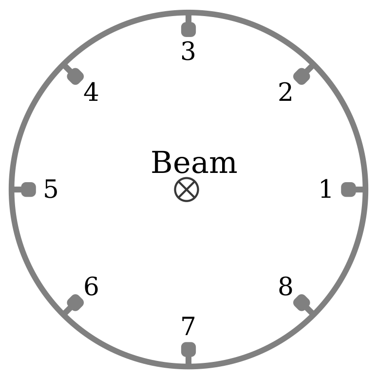
Figure 1: Sketch of a button BPM cross section. The numbers indicate the pick-up electrodes.

2 Multipole analysis

The beam profile monitor (BPM) in this work includes eight pick-up electrodes, uniformly distributed around the beam (Figure 1). An incoming beam generates a signal on the electrodes, which depends on its transverse distribution and the current it carries. The induced current on an electrode by a delta function line current is given in the cylindrical coordinates as [18]

$$J_{\textnormal{image}}(r,\phi,a,\theta)=\frac{I(r,\phi)}{2\pi a}\frac{a^{2}-r^{2}}{a^{2}+r^{2}-2ar\cos(\theta-\phi)},$$ (1)

where $I$ is the beam current, $a$ and $\phi$ are the radial position and the azimuthal angle of the electrode, $r$ and $\theta$ are those of the beam, respectively. Expanding it in powers of $r/a$, one obtains

$$J_{\textnormal{image}}(r,\phi,a,\theta)=\frac{I(r,\phi)}{2\pi a}\left[1+2\sum_{k=1}^{\infty}\left(\frac{r}{a}\right)^{k}\cos k(\theta-\phi)\right].$$ (2)

This formalism can naturally be extended to an arbitrary beam profile distribution by integration. For a Gaussian charge distribution with standard deviations $\sigma_{x}$ and $\sigma_{y}$, centered at $\bar{x}$ and $\bar{y}$, it becomes

$$J_{\textnormal{image}}(a,\theta)=\frac{I_{\textnormal{beam}}}{4\pi^{2}a\sigma_{x}\sigma_{y}}\iint_{\textnormal{beam}}\left[1+2\sum_{k=1}^{\infty}\left(\frac{r}{a}\right)^{k}\cos k\left(\theta-\phi\right)\right]\\ \exp\left[\frac{{\left(x-\bar{x}\right)}^{2}}{2\sigma_{x}^{2}}\right]\exp\left[\frac{{\left(y-\bar{y}\right)}^{2}}{2\sigma_{y}^{2}}\right]dA,$$ (3)

where $k$ is the order of the multipoles. Further expanding with $k$ for $r<a$ gives

$$\begin{split}J_{\textnormal{image}}(a,\theta)\approx\frac{I_{\textnormal{beam}}}{2\pi a}&\Bigg{(}1+2\left[\frac{\bar{x}}{a}\cos\theta+\frac{\bar{y}}{a}\sin\theta\right]+2\left[\left(\frac{\sigma_{x}^{2}-\sigma_{y}^{2}}{a^{2}}+\frac{\bar{x}^{2}-\bar{y}^{2}}{a^{2}}\right)\cos 2\theta+2\frac{\bar{x}\bar{y}}{a^{2}}\sin 2\theta\right]\\ &+2\left[3\left(\frac{\sigma_{x}^{2}-\sigma_{y}^{2}}{a^{2}}\right)+\frac{\bar{x}^{2}-\bar{y}^{2}}{a^{2}}\right]\left(\frac{\bar{x}}{a}\cos 3\theta+\frac{\bar{y}}{a}\sin 3\theta\right)+\cdots\Bigg{)},\end{split}$$ (4)

where higher order terms are omitted as an approximation for a pencil beam in which $\sigma_{x,y}$ is small compared to the beam pipe radius [18]. Nevertheless, the main operational equation of this work is Equation 1; hence free of approximations.

It is clear that two beams with different profiles can induce the same signal if their $\sigma^{2}=\sigma_{x}^{2}-\sigma_{y}^{2}$ and $\bar{x}^{2}-\bar{y}^{2}$ are the same. This causes degenerate solutions, which result in arbitrary changes in the size of the reconstructed beam. This systematic error can be reduced with knowledge of the beam size, or alternatively beam emittances ($\epsilon_{x,y}$) and beta functions ($\beta_{x,y}$). In the proton EDM experiment, the beam size is expected to be known precisely thanks to the continuous beam extraction. Effect of the $\epsilon_{x,y}$ and $\beta_{x,y}$ drifts is analyzed in the A.

3 Beam profile reconstruction routine

An arbitrary beam profile with $N$ particles of $(x,y)$ coordinates can be represented by a $2\times N$ matrix X. The beam induces a signal, which is represented by an 8-dimensional vector Y, on the eight electrodes of the BPM (Figure 1). A sample beam of $N=10^{4}$ particles and the corresponding signal on the electrodes are shown in Figure 2.

Before presenting the reconstruction algorithm, prerequisite sections are listed first — Section 3.1 and 3.2. The main algorithmic routine is then thoroughly discussed in Section 3.3.

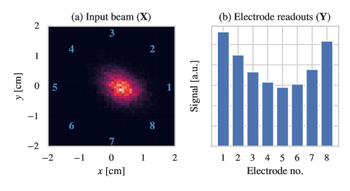
Figure 2: (a) A beam profile is represented by a $2\times N$ matrix X. The numbers from 1 to 8 represent the locations of the electrodes. The color code indicates the intensity of particles, where bright colors indicate higher intensity. (b) The induced signal on the electrodes is represented by an 8-dimensional vector Y.

3.1 Beam manipulation operators

The algorithm slowly “steers” a randomly generated Gaussian beam toward its “true” position and shape. This transformation is accomplished through several operators, which modify the position $(x,y)$ of each particle in the beam. The transformations are made in small steps ( $\delta_{x,y}$) for better accuracy and stability. The list of the operators are as follows:

• Translation: This operator is required for finding the correct beam position.

  $$(x,y)\longrightarrow(x\pm\delta_{x},\quad y),$$ (5)

  $$(x,y)\longrightarrow(x,\quad y\pm\delta_{y}).$$ (6)

• Scaling: The beam size and shape change by stretching the beam with respect to its center.

  $$(x,y)\longrightarrow(x\cdot(1\pm\delta_{x}),\quad y),$$ (7)

  $$(x,y)\longrightarrow(x,\quad y\cdot(1\pm\delta_{y})).$$ (8)

• Shearing: This operator introduces a coupling between the $x$ and $y$ distributions, hence a rotation.

  $$(x,y)\longrightarrow(x\cdot(1\pm y\delta_{x}),\quad y),$$ (9)

  $$(x,y)\longrightarrow(x,\quad y\cdot(1\pm x\delta_{y})).$$ (10)

• Bending: This operator helps achieving a variety of distortions.

  $$(x,y)\longrightarrow(x\cdot(1\pm\textnormal{abs}(y)\cdot\delta_{x}),\quad y),$$ (11)

  $$(x,y)\longrightarrow(x,\quad y\cdot(1\pm\textnormal{abs}(x)\cdot\delta_{y})).$$ (12)

As an example, by means of Equations 5 and 6, a test beam X${}^{\textnormal{try}}$ moves by $(\pm\delta_{x},\pm\delta_{y})$, chasing the minimum value of the loss function, and settles where it minimizes. The method is heavily inspired by the gradient descent [25] and simulated annealing [26] algorithms. All the operations are applied in parallel, and the best operation is selected according to the resulting loss function. The resulting state of the beam profile most likely sits at a local minimum. As mentioned above, we are using the genetic algorithm to introduce a randomness and an escape mechanism from the local minima.

It is clear that this is not the ultimate list of operators for beam transformations. For instance, an “S-shaped” beam cannot be produced by them from an initially Gaussian beam. This limitation does not appear in our study because both the test beam profiles (X${}^{\textnormal{true}}$) and the reconstructed profiles (X${}^{\textnormal{try}}$) are generated by modifying a Gaussian beam by the same operators. However, this does not invalidate the conclusions of this study as long as one can define operators relevant to a particular shape.

Finally, as mentioned above, the ambiguity from $\sigma_{x}^{2}-\sigma_{y}^{2}$ also limits the performance of the algorithm. Therefore, we introduced beam size knowledge at the loss function to favor solutions that are compatible with a presumed beam size.

3.2 Loss function

The search algorithm accepts or rejects a transformation according to its loss function. Choice of a loss function is somewhat an arbitrary procedure, and can affect the performance significantly. It is composed of two parts in this routine.

The first part is the mean square error (MSE) of the signal that is induced at the electrodes:

$$\textnormal{MSE}(\textbf{Y}^{\textnormal{try}},\textbf{Y}^{\textnormal{true}})=\frac{1}{N_{e}}(\textbf{Y}^{\textnormal{try}}-\textbf{Y}^{\textnormal{true}})(\textbf{Y}^{\textnormal{try}}-\textbf{Y}^{\textnormal{true}})^{\textbf{T}},$$ (13)

where $N_{e}$ is the number of electrodes, Y${}^{\textnormal{true}}$ and Y${}^{\textnormal{try}}$ represent the true signal and the signal obtained after transformation, respectively, and T is the transpose of the matrix.

The degeneracy problem requires a knowledge of the beam dimensions, $\langle x^{2}\rangle$ and $\langle y^{2}\rangle$. The second part of the loss function, so-called exponential penalty (EP), is given as

$$\begin{split}\Delta_{x}&\equiv\left(\sqrt{\langle x^{2}\rangle^{\textnormal{try}}}-\sqrt{\langle x^{2}\rangle}\right)^{2},\\ \Delta_{y}&\equiv\left(\sqrt{\langle y^{2}\rangle^{\textnormal{try}}}-\sqrt{\langle y^{2}\rangle}\right)^{2},\\ \textnormal{EP}(\textbf{Y}^{\textnormal{try}},\textbf{Y}^{\textnormal{true}})&=\exp(w\Delta_{x})+\exp(w\Delta_{y}),\end{split}$$ (14)

where $w$ is practically the relative weight of the EP term. Then, the combined loss function becomes

$$L(\textbf{Y}^{\textnormal{try}},\textbf{Y}^{\textnormal{true}})=\textnormal{MSE}(\textbf{Y}^{\textnormal{try}},\textbf{Y}^{\textnormal{true}})+\textnormal{EP}(\textbf{Y}^{\textnormal{try}},\textbf{Y}^{\textnormal{true}}),$$ (15)

The EP favors the solutions that have a size similar to the given beam size. If the loss function is purely EP, then the algorithm converges to a Gaussian beam with the correct beam size, but loses the profile and position information. In contrast, if it is purely MSE, then the algorithm likely converges to one of the degenerate solutions with an arbitrary size. According to our tests, $w\approx 10^{4}$ yields acceptable results for a wide range of beam profiles. However, with a prior knowledge of the approximate beam profile or the beam size, it can be readjusted to boost the performance. It can also be calibrated by independent measurements of other BPMs as well. It is worth emphasizing again that the choice of the operators, $\pm\delta_{x,y}$, and $w$ is rather arbitrary and should vary at different applications.

Another approach is to generate the reproduction candidates solely via the MSE and eventually filter them by the EP according to the beam size. However, this approach suffers from unnecessary steering of the beam profile toward unlikely $\langle x^{2}\rangle$ and $\langle y^{2}\rangle$ values during the minimization process. We found it computationally beneficial to embed the EP into the loss function.

3.3 Algorithm

The reconstruction routine is depicted in Figure 3. Initially, a random beam (X${}^{\textnormal{true}}$) with an arbitrary distortion is created and the corresponding Y${}^{\textnormal{true}}$ is calculated for reference. In a real BPM measurement, only Y${}^{\textnormal{true}}$ will be known. Then, a minimization algorithm starts with $n=50$ candidate Gaussian beams of random shapes and locations, represented with X_1→n. Each beam induces signals on the probes, shown with the vector Y${}^{\textnormal{try}}$. The beams are transformed in parallel by several operators one-by-one to achieve signals as close as possible to the given Y${}^{\textnormal{true}}$. The above procedures do not guarantee the correct beam profile because it may be stuck at a local minimum. Then, according to their loss function values, $n$ solutions are selected for mutation. In contrast to the cross breeding of the genetic algorithm [27], the next generation beams are selected randomly, with probabilities inversely proportional to the loss function. This is also known as “roulette wheel selection” or “fitness proportionate selection”. Note that in this selection, some solutions $G_{i}$ may be selected multiple times and some others may not be selected at all. Then, the selected candidates are mutated by randomly applying one of the operators of Section 3.1, only with a higher amplitude. The last step ensures that the candidates are steered away from the local minima. This completes the iteration and the $n$ newly generated beam profiles are returned as starting candidates for the next iteration. Algorithm 1 summarizes the process in pseudo code.

Figure 3: The reconstruction routine is composed of several layers of operations. Firstly, $n$ random beams are initialized and then transformed by a gradient descent-like method to reach minima, either local or global. Then, some solutions are selected according to their loss functions, and mutated for the next iteration.

Input: Y${}^{\textnormal{true}}$

Output: X${}^{\textnormal{try}}$

Initialize $n$ parallel instances of randomly generated beams X_1→n

for iterations do

       foreach X_1→n do

             /* Search for local minimum */

             repeat

                   $\mathbf{Y}_{1\rightarrow n}=J_{\textnormal{image}}(\mathbf{X}_{1\rightarrow n})$ from Equation 1

                   $\mathbf{X}_{1\rightarrow n}^{\textnormal{try}}$ = [$f(\mathbf{X}_{1\rightarrow n})$ for $f$ in operators specified in Section 3.1] /* Transform the beams */

                   $\mathbf{Y}_{1\rightarrow n}^{\textnormal{try}}=J_{\textnormal{image}}(\mathbf{X}_{1\rightarrow n}^{\textnormal{try}})$ /* Electrode signals after transformation */

                  

            until $L(\mathbf{Y}_{1\rightarrow n}^{\textnormal{try}},\mathbf{Y^{\textnormal{true}}})<L(\mathbf{Y}_{1\rightarrow n},\mathbf{Y^{\textnormal{true}}})$ is found

            /* $L$ is the loss function, defined in Section 3.2 */

             $\mathbf{G}_{1\rightarrow n}=\mathbf{X}_{1\rightarrow n}^{\textnormal{try}}$

            

      /* At this point, every $\mathbf{X}_{1\rightarrow n}$ is transformed to a $\mathbf{G}_{1\rightarrow n}$ that represents a minimum */

       Select $n$ solutions S_1→n from G_1→n

       Mutate $\mathbf{S}_{1\rightarrow n}$ for the next iteration: $\mathbf{S}_{1\rightarrow n}\longrightarrow\mathbf{X}_{1\rightarrow n}$

      

Algorithm 1 Initially, a test beam X${}^{\textnormal{true}}$ is created and the corresponding signal Y${}^{\textnormal{true}}$ on the electrodes is calculated. The algorithm aims to reconstruct X${}^{\textnormal{true}}$ from a set of randomly generated beams, by transforming them in parallel, which eventually induce Y${}^{\textnormal{true}}$. It makes use of a genetic algorithm with a gradient descent-like minimization. A schematic view of the algorithm is given in Figure 3.

We attempted mapping X onto Y by means of data-driven deep neural networks as well (More about this in B). Such a method, however, biases the predictions toward previously seen data and is unable to predict unencountered beam profile shapes. Eventually, we found the performance of the presented method to be superior not only because it requires no precursory training, but also it produces more robust results, free of possible neural network artifacts.

4 Reconstruction tests

For every test, we determined a “true” beam of random shape and position, which had a “true” signal on the electrodes. Then, we followed the algorithm that was explained in Section 3 for reconstruction. At the end, comparison between the true and reconstructed beams ($\textbf{X}^{\textnormal{true}}$ and X${}^{\textnormal{rec}}$, respectively) is made by using Structural Similarity Index Measure (SSIM), which is defined as

$$\textnormal{SSIM}(\textbf{X}^{\textnormal{true}},\textbf{X}^{\textnormal{rec}})=\frac{(2\mu_{\textnormal{t}}\mu_{\textnormal{r}}+C_{1})(2\sigma_{\textnormal{tr}}+C_{2})}{(\mu_{\textnormal{t}}^{2}+\mu_{\textnormal{r}}^{2}+C_{1})(\sigma_{\textnormal{t}}^{2}+\sigma_{\textnormal{r}}^{2}+C_{2})}.$$ (16)

Here, $\mu$ and $\sigma$ are the mean and the standard deviation of the pixel brightness, subscripts ‘t’ and ‘r’ represent “true” and “reconstructed” respectively. $\sigma_{\textnormal{tr}}$ refers to covariance of ‘t’ and ‘r’. $C_{1}$ and $C_{2}$ are normalization constants. The SSIM score ranges from -1.0 to 1.0, with the latter corresponding to an identical copy.

Rather than calculating Equation 16 once for the whole images, they are split into sub-regions and the calculations are made at that scale. Then, the SSIM scores are averaged over the individual sub-region pairs, weighted with a circular Gaussian filter of $1.5\sigma$. The SSIM is preferable for a 2D image comparison since it mimics human preception. More detailed discussion on SSIM, selection of the coefficients and the sub-regions, and a comparison with MSE of Equation 13 can be found at References [28] and [29].

As mentioned in Section 3.2, the beam size knowledge plays an important role in the reconstruction routine. For every test, we have also applied the reconstruction algorithm with incorrect beam size values to see how the performance degrades. Figure 4 shows a variety of test beams (the leftmost column) and the corresponding reconstructions with increasing errors in the beam size knowledge at every column. The beam size errors correspond to $\sigma_{x}$ and $\sigma_{y}$ at the same time, because the reconstruction error becomes less if one of them has a smaller error.

Elongated beams have a clear quadrupole moment, which is relatively easy to pick up by the electrodes. Therefore, they can be perfectly reconstructed if the beam size is known well (Row 1). With an increase in the beam size error, the beam becomes thicker while $\sigma_{x}^{2}-\sigma_{y}^{2}$ remains the same. This effect becomes more visible with beam size errors larger than 20%. The signal at the electrodes do not vary much for round beams (Row 2). Therefore, the algorithm works very well if the beam size is known well. Otherwise, the beam shape is protected except for very small beams, while its size changes in proportion to the beam size error. This effect is also barely visible for 10% level beam size error. While distorted beams (as shown in Rows 3, 4, and 5) can also be reconstructed quite precisely, there are occasional cases that banana shapes are interpreted as triangular, and vice versa. This originates from the similarity of the probe signals for each case. It is worth noting that <10% beam size error, where the BPM performs quite well for all studied profiles, is reasonable for the proton EDM experiment. More details on this are given in the A. Figure 5 shows the SSIM comparison between the test beam and the reconstructed beams for an ensemble of 500 particles with random profiles. Comparison with Figure 4 shows that a SSIM score around 0.95 and beyond usually indicates a perfect match, which is likely to be achieved with good knowledge of the beam size. For the 10% beam size error, majority of the reconstructed profiles have SSIM scores better than 0.90. The results get significantly better at 6% beam size error and below.

Finally, as confirmed by additional simulations, the SSIM score is not seriously affected by up to $\pm 3\%$ random probe noise — Figure 6. Such random probe noise is added to imitate real life total noise levels. It is equally important how such noise translates to voltage levels in a realistic physical design. Assuming that the thermal noise contribution would be around,

$$v_{n}=\sqrt{4k_{B}TR\Delta f}=\sqrt{4\cdot 1.38\cdot 10^{-23}~{}\mathrm{J}/\mathrm{K}\cdot 300~{}\mathrm{K}\cdot 50\Omega\cdot 100~{}\mathrm{MHz}}=9~{}\mu\textrm{V}.$$

$50~{}\Omega$ corresponds to pickup grounding impedance and $100~{}\mathrm{MHz}$ corresponds to expected (conservative) bandwidth. The voltage signal ($I_{\textnormal{beam}}\cdot Z_{\mathrm{transfer}}$) including the aforementioned acceptable 3% noise would be,

$$1.7~{}\mathrm{mA}\cdot Z_{\mathrm{transfer}}\cdot 0.03=51~{}\mu\textrm{V},$$

where the transfer impedance was assumed to be $Z_{\mathrm{transfer}}=1\Omega$ as a reference. In such a configuration, the expected power signal-to-noise ratio is 31. As the bunches 1-to-80 are supposed to be similar at each turn, averaging over those bunches can be considered for further improvement.

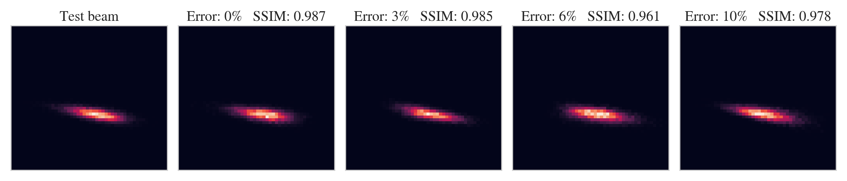
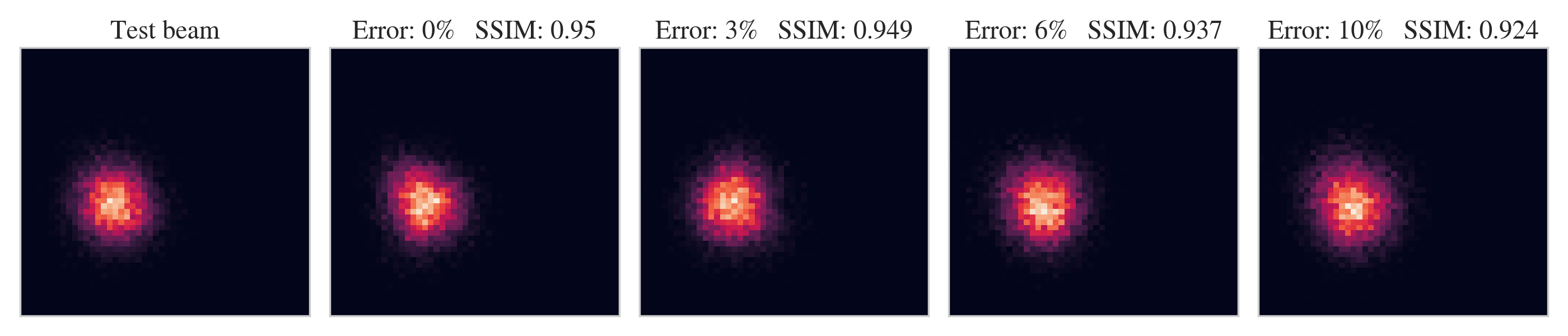
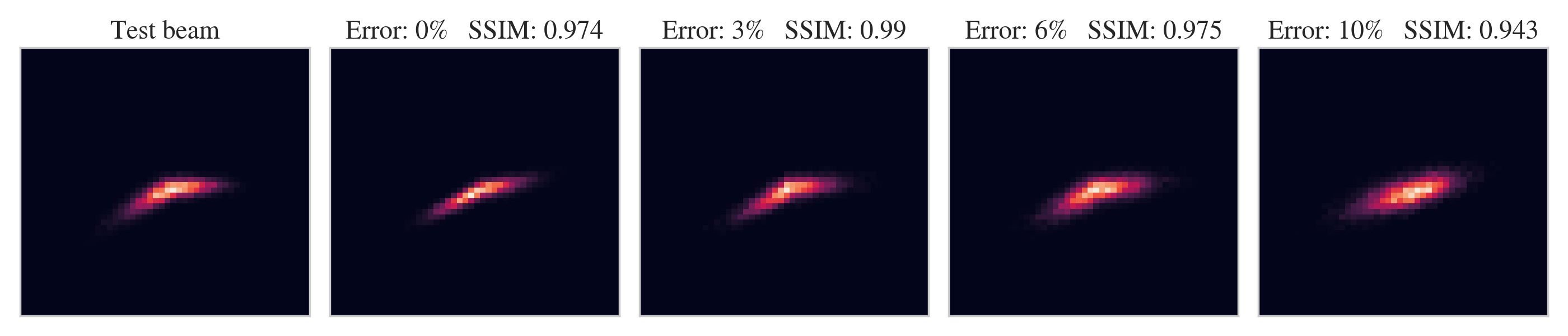
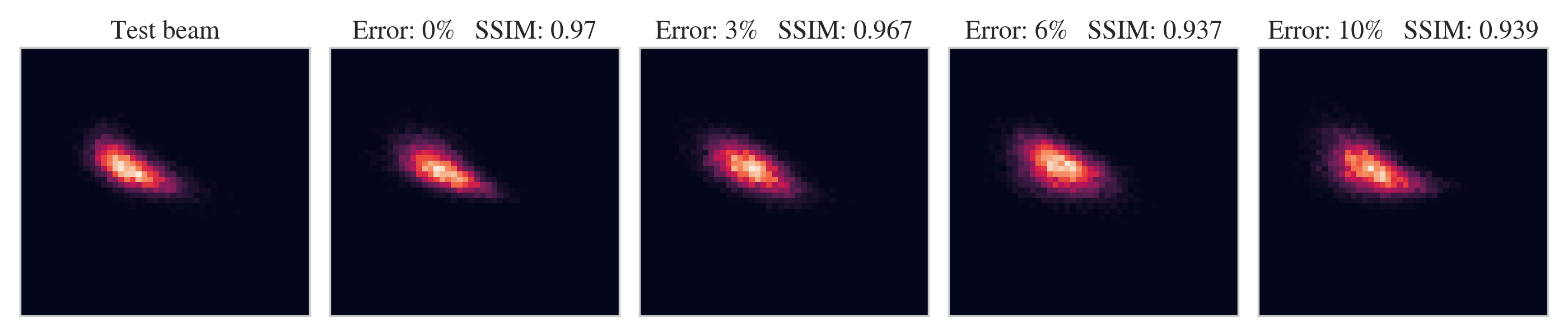
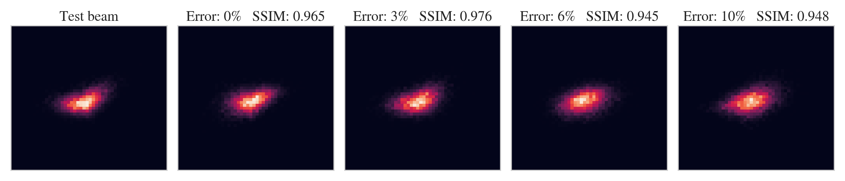
Figure 4: Test beam profiles and the reconstructed beam profiles for different cases. Location of the probes and the scale of the images are identical with Figure 2. Each row corresponds to a separate test beam, given in the first column. The columns on the right correspond to beams with size errors ranging between 0% and 10%. SSIM of each solution, compared to the test beam is shown above the images as reference. Figure 5 shows the overall SSIM results for a larger ensemble.

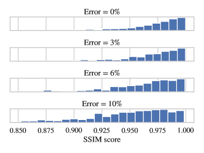
Figure 5: Histogram of SSIM vs. beam size error, which is obtained from 500 test beams. The method performs effectively when the beam size is known well. The tail is likely to originate from the extremely distorted beams, which is always harder to reconstruct. The method yields acceptable results up to 10% error, while it performs quite better at lower errors.

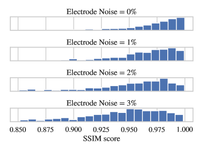
Figure 6: Histogram of SSIM vs. random rms $\sigma$ probe noise, which is obtained from 500 test beams. Random rms $\sigma=$0–3% noise is applied on each of the 8 probes of the profile monitor. The quality of the results (SSIM score) does not seem to degrade significantly.

5 Summary and conclusion

We presented a novel non-destructive beam profile visualization technique that requires a button beam position monitoring hardware and machine learning enhanced data processing. Genetic algorithm starts off with an array of first generation random beam profiles which are then transformed by successive application of transformations (given in Section 3.1) toward the minimal loss function (Equation 15). Once the entire generation of beam profiles reach their respective local minima, several beam profiles are selected randomly with probabilities inversely proportional to their loss functions, reproduced, and then mutated toward use in the next generation. This process repeats for a predetermined number of generations. The major limitation is the degeneracy due to $\sigma_{x}^{2}-\sigma_{y}^{2}$. In principle, it can be eliminated with a perfect knowledge of the beam size. In the proton EDM experiment, the error in beam size estimation is expected to be known within a few percent because of continuous extraction. Depending on the application, additional beam transformation operators that are more compatible with the presumed beam profiles can be implemented. A simplified code and an example are given at Refs [30] and [31], respectively.

6 Acknowledgments

This work was supported by IBS-R017-D1 of the Republic of Korea. We would like to thank Yannis K. Semertzidis for helpful discussions. We would also like to thank Changkyu Sung for pointing the degeneracy problem due to the quadrupole moment, and Sanzhar Bakhtiyarov and Adil Karjauv for helpful discussions on machine learning algorithms.

Appendix A Beam size and effect of the $\beta$ and $\epsilon$ drifts

The pEDM storage ring is composed of 24 cells, each having electric deflectors, drifts, sextupoles, and focusing and defocusing magnetic quadrupoles as depicted in Figure 7. The beta functions are symmetric at every cell as shown in Figure 8, which covers two cells with the quadrupoles and the BPM indicated. The emittances of the beam are $\epsilon_{x}=0.214$ mm-mrad and $\epsilon_{y}=0.25$ mm-mrad. The beam will be continuously extracted during storage at the polarimeter target. Therefore, its size will be fixed at that location. Upon beta function measurements, it can also be estimated at other locations.

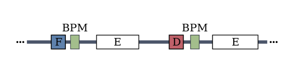
Figure 7: A FODO cell with electric deflectors (E), focusing (F) and defocusing (D) quadrupoles, BPM’s, and straight sections (gray lines). Sextupoles overlap with quadrupoles.

Some storages in the experiment will periodically be dedicated to beam and field diagnostics, and field corrections, instead of EDM measurements. Beta functions can as well be determined at those diagnostic storages. According to our studies, the emittance growth time is roughly 40 minutes in all directions. Combined with continuous extraction, this guarantees a fixed beam size at the polarimeter location during storage ($\approx 20$ minutes). However, the stability of the quadrupoles in long term may be a concern as it has an effect on the beam size. This is investigated in two ways by i) changing the focusing strength of the neighbor quadrupole, and ii) randomly changing the focusing strength of all the quadrupoles. Note that these scenarios refer to quadrupole strength variations at the EDM measurement storages.

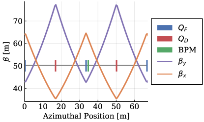
Figure 8: Beta functions in two cells. The focusing and defocusing quadrupoles are shown with blue and red vertical lines. The BPM (shown in green) is located 1 m away from the quadrupole.

The RMS beam size is roughly determined by the emittance $\epsilon$ and the beta function $\beta$ as

$$\begin{split}\sigma_{x}^{2}\propto\langle x^{2}\rangle&=\epsilon_{x}\beta_{x},\\ \sigma_{y}^{2}\propto\langle y^{2}\rangle&=\epsilon_{y}\beta_{y},\end{split}$$

where $x$ and $y$ are the horizontal and vertical positions with respect to the beam center, respectively. The brackets represent average over particles in the beam, and the subscripts represent the horizontal or vertical directions. The ratio of the horizontal beam size to the vertical is

$$\frac{\sigma_{x}^{2}}{\sigma_{y}^{2}}=R_{\epsilon}R_{\beta},$$

where $R_{\epsilon}\equiv\epsilon_{x}/\epsilon_{y}$ and $R_{\beta}\equiv\beta_{x}/\beta_{y}$. Then, one gets

$$\sigma^{2}= \left(R_{\epsilon}R_{\beta}-1\right)\sigma^{2}_{y},$$

$$\sigma^{2}_{y}= \frac{\sigma^{2}}{R_{\epsilon}R_{\beta}-1},$$

$$\sigma^{2}_{x}= \sigma^{2}\left(1+\frac{1}{R_{\epsilon}R_{\beta}-1}\right).$$

$\sigma^{2}$ is obtained by the BPM, and $R_{\epsilon}$ and $R_{\beta}$ are given either by analytical estimations or independent measurements. The error in $\sigma_{x}^{2}$ and $\sigma_{y}^{2}$ is

$$\delta\sigma^{2}_{x,y}=-\frac{R_{\epsilon}\delta R_{\beta}+R_{\beta}\delta R_{\epsilon}}{(R_{\epsilon}R_{\beta}-1)^{2}}\sigma^{2},$$ (17)

where $\delta R_{\epsilon}$ and $\delta R_{\beta}$ are the errors of $R_{\epsilon}$ and $R_{\beta}$ estimations, respectively. $\delta R_{\beta}$ is defined as

$$\delta R_{\beta}=\frac{\delta\beta_{x}}{\beta_{y}}-\frac{\beta_{x}\delta\beta_{y}}{\beta_{y}^{2}},$$ (18)

where $\delta\beta_{x,y}$ are the errors on the beta functions. Setting $\delta\beta_{x}=b_{x}\beta_{x}$ and $\delta\beta_{y}=b_{y}\beta_{y}$, Equation 18 simplifies to $\delta R_{\beta}=(b_{x}-b_{y})R_{\beta}$. Similarly, by using $\delta\epsilon_{x}=a_{x}\epsilon_{x}$ and $\delta\epsilon_{y}=a_{y}\epsilon_{y}$, one gets $\delta R_{\epsilon}=(a_{x}-a_{y})R_{\epsilon}$. Inserting $\delta R_{\beta}$ and $\delta R_{\epsilon}$ into Equation 17, one obtains

$$\delta\sigma^{2}_{x,y}=-\frac{R_{\epsilon}R_{\beta}(a_{x}-a_{y}+b_{x}-b_{y})}{(R_{\epsilon}R_{\beta}-1)^{2}}\sigma^{2}.$$ (19)

For the lattice proposed at Ref [2], $R_{\epsilon}\approx 0.9$ and $R_{\beta}$ is 1.5 or 0.47, depending on the BPM location. As a result, one half cell is roughly an order of magnitude more sensitive than the other to the emittance and beta function drifts. Figure 9 shows the variation of the emittances, beta functions, and the beam size (from Equation 19) for the “worse” half cell as a function of variations of the neighboring quadrupole strength ($\Delta k/k$). The data is obtained by one-particle beam dynamics simulations inside the storage ring of Ref [2]. Beam stability and resonance issues are not considered in this treatment. The change in the beam size is almost linearly proportional to $\Delta k/k$, and it is at the same order of the changes in the beta functions and the emittances. 10% change in $\Delta k/k$, resulting in 10% change in the beam size, is quite tolerable for the BPM as shown in Figures 4 and 5.

The focusing strength of each quadrupole can vary randomly as well. Assuming a Gaussian variation with 0.1% standard deviation ($\sigma^{\Delta k/k}=10^{-3}$), we made 500 simulations with single particles to obtain the histogram in Figure 10, which indicates that the relative beam size variation is most likely within a few percent in this scenario. In conclusion, the proposed BPM is tolerable to random quadrupole strength drifts as long as they are within $\pm 0.1\%$, and one quadrupole failure as long as the drift is less than 10% level.

Appendix B Profile reconstruction attempt using neural networks

The neural network (NN) of choice was a dense Y to X fully connected with a few layers. A continuous funnel-shaped Y (8 dims) to X ($20000=2\times 10000$ dims) with up to 10 fully connected layers NNs were tested. The size (both depth and width) did not seem to affect the performance as much.

Keras [32] package was used to construct and train the network. Standard procedures like L1,L2 normalization; early stopping; random dropoff were implemented. The initial idea to use SSIM loss function came from various modifications to NN setup. SSIM loss function, although costlier than MSE, vastly outperformed MSE in terms of quality of the results.

Roughly $10^{6}$ (X, Y) pairs were used in the training stage. The training data consisted only from well-shaped 2-d gaussian beams (no distortions). NNs perform acceptably when the training data and the testing data are sampled from the same distribution (same data generating function). However, when some distortion (bending the beams for example (as in Figure 4)) is introduced (roughly in 10% of the samples) in either in the test or training samples, the results become unacceptable. Simple-to-reconstruct shapes are misinterpreted as more complex shapes and vice-versa. Absence of robustness despite the large training sample and time-consuming training made us rethink the approach. The proposed genetic algorithm requires no prior training (although fine-tuned beforehand); has interpretable logic; is more performant.

Though convolution layers (or other popular choices like transformers) might seem tempting to use, the problem at hand is reversed — we need to go from low dimensional data Y to high dimensional data X.

A few additional details that are worth mentioning:

1. The order of the data point pairs in X is irrelevant. Any permutation of the charged particle locations leads to the same signal. This hints that usage of permutation invariant Graph Neural Networks or Set Transformers might be possible as an extension for future studies. However, using such state-of-the art models seems to be an overkill for such clear-stated problem.

2. We expect physically relevant beam profile data X to be continuous (without holes or tears) blobs with approximately Gaussian distribution. To our knowledge, there does not seem to be an analytical,as well as back propagation compatible, function to enforce this. However, the operators (Section 3a) conserve such continuousness naturally.

Another idea, was to use a somewhat middle ground approach — Reinforcement Learning (RL). RL has not been attempted, but it could also be a natural step toward future extension.

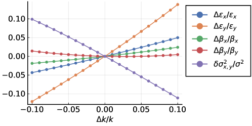
Figure 9: The change in the beta functions, emittance, and the beam size as the quadrupole strength next to the BPM is varied.

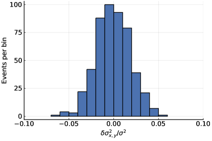
Figure 10: Histogram of beam size error as the strength of every quadrupole is varied randomly by $\sigma^{\Delta k/k}=0.1\%$. The histogram is obtained by five hundred single particle dynamics simulations with different seeds. In 95% of the cases, the beam size error $\Delta\sigma_{x,y}^{2}/\sigma^{2}$ is within $\pm 3\%$.

References

- [1] V. Anastassopoulos et al., A storage ring experiment to detect a proton electric dipole moment, Review of Scientific Instruments 87 (2016) 115116.
- [2] Z. Omarov, S. Haciomeroglu, V. Lebedev, W.M. Morse, A.J Silenko, E.J. Stephenson, Y.K. Semertzidis, Comprehensive Symmetric-Hybrid ring design for pEDM experiment at below cm, 2020, arXiv:2007.10332.
- [3] Ch. Steinbach and M. van Rooij, A Scanning Wire Beam Profile Monitor, IEEE Transactions on Nuclear Science 32 (1985) 1920-1922.
- [4] S. Igarashi, D. Arakawa, K. Koba, H. Sato, T. Toyoma, M. Yoshii, Flying wire beam profile monitors at the KEK PS main ring, Nuclear Instruments and Methods in Physics Research Section A: Accelerators, Spectrometers, Detectors and Associated Equipment 482 (2002) 32-41.
- [5] D.G. Seely, H. Bruhns, D.W. Savin, T.J. Kvale, E. Galutschek, H. Aliabadi, C.C. Havener, Rotating dual-wire beam profile monitor optimized for use in merged-beams experiments, Nuclear Instruments and Methods in Physics Research Section A: Accelerators, Spectrometers, Detectors and Associated Equipment 585 (2008) 69-75.
- [6] G.L. Orlandi, et al., Design and test of wire-scanners for SwissFEL, 2016, arXiv:1611.00151.
- [7] V.W. Yuan, R.C. Connolly, R.C. Garcia, K.F. Johnson, K. Saadatmand, O.R. Sander, D.P. Sandoval, M.A. Shinas, Measurement of longitudinal phase space in an accelerated H- Beamusing a laser-induced neutralization method, Nuclear Instruments and Methods in Physics Research Section A: Accelerators, Spectrometers, Detectors and Associated Equipment, 329 (1993) 381-392.
- [8] H. Sakai, Y. Honda, N. Sasao, S. Araki, Y. Higashi, T. Okugi, T. Taniguchi, J. Urakawa and M. Takano, Performance Studies of a Laser Wire Beam Profile Monitor, Japanese Journal of Applied Physics 41 (2002) 6398-6408.
- [9] DeLuca, William H, Beam detection using residual gas ionization, IEEE Transactions on Nuclear science 16, no. 3 (1969): 813-822.
- [10] Connolly, R., Cameron, P., Ryan, W., Shea, T.J., Sikora, R. and Tsoupas, A prototype ionization profile monitor for RHIC, Proceedings of the 1997 Particle Accelerator Conference (Cat. No. 97CH36167) (Vol. 2, pp. 2152-2154). IEEE.
- [11] Y. Hashimoto, T. Fujisawa, T. Morimoto, Y. Fujita, T. Honma, S. Muto, K. Noda, Y. Sato, S. Yamada, Oxygen gas-sheet beam profile monitor for the synchrotron and storage ring, Nuclear Instruments and Methods in Physics Research Section A: Accelerators, Spectrometers, Detectors and Associated Equipment 527 (2004) 289-300.
- [12] T. Honma, D. Ohsawa, K. Noda, T. Iwashima, H.Y. Ogawa, Y. Sano, E. Takada, S. Yamada, Design and performance of a non-destructive beam-profilemonitor utilizing charge-division method at HIMAC, Nuclear Instruments and Methods in Physics Research Section A: Accelerators, Spectrometers, Detectors and Associated Equipment 490 (2002) 435-443.
- [13] L. Cosentino, A. Musumarra, M. Barbagallo, N. Colonna, L. Damone, A. Pappalardo, M. Piscopo and P. Finocchiaro, Silicon detectors for monitoring neutron beams in n-TOF beamlines, Review of Scientific Instruments 86 (2015) 073509.
- [14] C.P. Welsch, E. Bravin, T. Lefevre, Investigations of OTR screens and shapes, Proceedings of EPAC06, Edinburg, Scotland, 2006, CERN-AB-2006-069.
- [15] U. Iriso, G. Benedetti, and F. Perez, Experience with YAG and OTR screens at ALBA, Proceedings of DIPAC09, Basel, Switzerland, 2009, TUPB15.
- [16] Mahan A.H., Gallagher A, Transition radiation for the diagnosis of low-energy electron beams, Review of Scientific Instruments. 1976 Jan;47(1):81-3.
- [17] Bosser J., Mann J., Ferioli G., Warts L., Optical transition radiation proton beam profile monitor, Nuclear Instruments and Methods in Physics Research Section A: Accelerators, Spectrometers, Detectors and Associated Equipment. 1985 Jul 15;238(1):45-52.
- [18] R.H. Miller, J.E. Clendenin, M.B. James, J.C. Sheppard, Nonintercepting emittance monitor, 12th International Conference of High Energy Accelerators, IL, USA, 1983, SLAC–PUB–3186, CONF–830822–39 5746569.
- [19] T. Suwada, Multipole Analysis of Electromagnetic Field Generated by Single-Bunch Electron Beams, Japanese Journal of Applied Physics 40 (2001) 890-897.
- [20] T. Suwada, M. Satoh, K. Furukawa, Nondestructive beam energy-spread monitor using multi-strip-line electrodes, Physical Review Special Topics - Accelerators and Beams 6 (2003) 032801.
- [21] A. Sounas, M. Gasior, T. Lefevre, A. Mereghetti, J. Olexa, S. Redaelli, G. Valentino, Beam size measurements based on movable quadrupolar pick-ups, 9th International Particle Accelerator Conference, Vancouver, BC, Canada, 2018, WEPAF080.
- [22] J.A. Seibert, Iterative reconstruction: how it works, how to apply it, Pediatric Radiology 44 (2014) (Suppl 3): S431-S439.
- [23] W. Stiller, Basics of iterative reconstruction methods in computed tomography: A vendor-independent overview, European Journal of Radiology 109 (2018) 147-154.
- [24] L.L. Geyer, U.J. Schoepf, F.G. Meinel, J.W. Nance, Jr, G. Bastarrika, J.A. Leipsic, N.S. Paul, M. Rengo, A. Laghi, A.N. De Cecco, State of the Art: Iterative CT Reconstruction Techniques, Radiology 276 (2) (2015) 339-357.
- [25] S. Ruder, An overview of gradient descent optimization algorithms, 2017, arXiv:1609.04747.
- [26] Van Laarhoven, Peter JM and Aarts, Emile HL, Simulated annealing: Theory and applications, Springer, 1987.
- [27] D. Whitley, A genetic algorithm tutorial, Statistics and Computing 4 (1994) 65-85.
- [28] Z. Wang, A.C. Bovik, Mean squared error: Love it or leave it? A new look at signal fidelity measures, IEEE signal processing magazine 26 (2009) 98-117.
- [29] Z. Wang, A.C. Bovik, H.R. Sheikh, E.P. Simoncelli, Image quality assessment: from error visibility to structural similarity, IEEE transactions on image processing 13 (2004) 600-613.
- [30] Available at https://github.com/isentropic/computational-beam-profile-imaging (Accessed in 2020).
- [31] Available at https://github.com/isentropic/computational-beam-profile-imaging/blob/main/notebooks/Example.ipynb (Accessed in 2020).
- [32] Chollet, François et al., Keras, https://keras.io, (Accessed in 2020).