Projection on particle number and angular momentum: Example of triaxial Bogoliubov quasiparticle states

Abstract

Background

Many quantal many-body methods that aim at the description of self-bound nuclear or mesoscopic electronic systems make use of auxiliary wave functions that break one or several of the symmetries of the Hamiltonian in order to include correlations associated with the geometrical arrangement of the system’s constituents. Such reference states have been used already for a long time within self-consistent methods that are either based on effective valence-space Hamiltonians or energy density functionals, and they are presently also gaining popularity in the design of novel ab-initio methods. A fully quantal treatment of a self-bound many-body system, however, requires the restoration of the broken symmetries through the projection of the many-body wave functions of interest onto good quantum numbers.

Purpose

The goal of this work is three-fold. First, we want to give a general presentation of the formalism of the projection method starting from the underlying principles of group representation theory. Second, we want to investigate formal and practical aspects of the numerical implementation of particle-number and angular-momentum projection of Bogoliubov quasiparticle vacua, in particular with regard of obtaining accurate results at minimal computational cost. Third, we want to analyze the numerical, computational and physical consequences of intrinsic symmetries of the symmetry-breaking states when projecting them.

Methods

Using the algebra of group representation theory, we introduce the projection method for the general symmetry group of a given Hamiltonian. For realistic examples built with either a pseudo-potential-based energy density functional or a valence-space shell-model interaction, we then study the convergence and accuracy of the quadrature rules for the multi-dimensional integrals that have to be evaluated numerically and analyze the consequences of conserved subgroups of the broken symmetry groups.

Results

The main results of this work are also threefold. First, we give a concise, but general, presentation of the projection method that applies to the most important potentially broken symmetries whose restoration is relevant for nuclear spectroscopy. Second, we demonstrate how to achieve high accuracy of the discretizations used to evaluate the multi-dimensional integrals appearing in the calculation of particle-number and angular-momentum projected matrix elements while limiting the order of the employed quadrature rules. Third, for the example of a point-group symmetry that is often imposed on calculations that describe collective phenomena emerging in triaxially deformed nuclei, we provide the group-theoretical derivation of relations between the intermediate matrix elements that are integrated, which permits for a further significant reduction of the computational cost of the method. These simplifications are valid whatever the number parity of the quasiparticle states and therefore can be used in the description of even-even, odd-mass, and odd-odd nuclei.

Conclusions

The quantum-number projection technique is a versatile and efficient method that permits to restore the symmetry of any arbitrary many-body wave function. Its numerical implementation is relatively simple and accurate. In addition, it is possible to use the conserved symmetries of the reference states to reduce the computational burden of the method. More generally, the ever-growing computational resources and the development of nuclear ab-initio methods opens new possibilities of applications of the method.

I Introduction

The concept of symmetry is essential to the analysis, discussion, and understanding of many natural phenomena Henley (1996). In physics, the notion of symmetry is associated with the existence of physical transformations that leave either the laws of physics or the properties of physical systems invariant Caulton (2015). We will focus here on invariances of the interactions between a system’s fundamental constituents under global space-time symmetry transformations, such as translations in time and space, rotations, inversion of space and time, etc, which depend on a number of global parameters. Through Noether’s first theorem Noether (1918); Kosmann-Schwarzbach (2011), such global invariances are connected to the conservation of energy, momentum, angular momentum, parity, particle number, etc.

From a mathematical perspective, the concepts of symmetry can be expressed within the language of group representation theory Wigner (1959); Hamermesh (1962); Tinkham (1992); McWeeny (2002); Löwdin (1967). In particular, for finite quantal systems such as the atomic nucleus, the labels of the irreducible representations (irreps) of the general symmetry group of the Hamiltonian can be used as good quantum numbers that characterize its eigenstates. As a consequence, there are selection rules for electromagnetic transitions in nuclei, and also for nuclear transmutations induced by the weak and strong nuclear forces.

When solving the nuclear many-body problem exactly, the resulting many-body wave function will automatically be an eigenstate of all symmetry operators that commutate with the Hamiltonian and among each other. In one way or another, however, the microscopic modeling of nuclei almost always requires an ansatz for the nuclear many-body wave function $|\Psi\rangle$ and also implies the construction of an effective many-body Hamiltonian $\hat{H}_{\text{eff}}$ adequate for the model vector space covered by all possible $|\Psi\rangle$. While $\hat{H}_{\text{eff}}$ is in general constructed to preserve the physical symmetries of the “bare” Hamiltonian, it is not straightforward to ensure that the model wave functions $|\Psi\rangle$ conserve the same symmetries.

The latter problem is particularly prominent in variational methods, within which the physical state is approximated by the trial wave function that gives the lowest expectation value of the effective Hamiltonian within the given variational set. Conserving the physical symmetries by artificially restricting the variational space to symmetry-conserving product states might at first sight appear advantageous as one keeps quantum numbers and selection rules. However, when making the simple ansatz of a single product wave function for the variational state as it is done in self-consistent mean-field methods, more often than not one finds that a symmetry-breaking wave function gives a larger binding energy than a symmetry-conserving one. This problem is known for long as the “symmetry dilemma”, a notion first coined by Löwdin Lykos and Pratt (1963) in the context of atomic physics.

This finding has many similarities with the phenomenon of spontaneous symmetry breaking Strocchi (2005) that is well known for infinite systems such as the ones treated in condensed-matter physics. While for those symmetry breaking is an observable feature of the physical systems under study, for finite self-bound systems such as atomic nuclei finding a symmetry-breaking state that has the lowest energy for a symmetry-conserving Hamiltonian might appear as an unwanted byproduct of the modeling.

Time has shown, however, that it is often possible to attribute a physical meaning to such symmetry-breaking model states. It has been understood in ever increasing detail since the 1950s Bohr (1976); Rowe (1970); Bohr and Mottelson (1998); Ring and Schuck (1980) that the pattern of excited states of many atomic nuclei can be easily and intuitively explained by making the assumption that the many-body wave function can in one way or another be separated into a part representing a specific geometrical arrangement of nucleons and a part that represents the orientation of this arrangement in space, and where only the latter respects the symmetries of the Hamiltonian. By contrast, the part of the wave function that represents the relative arrangement of the nucleons then typically breaks some, but not necessarily all, of these symmetries. We will call those that remain intrinsic symmetries in what follows. They leave a characteristic fingerprint on the excitation spectrum of the system and are customarily used to characterize the distribution of nucleons as having a “spherical”, “axially deformed”, “triaxial”, “octupole deformed”, …shape Rowe (1970); Bohr and Mottelson (1998); Ring and Schuck (1980); Frauendorf (2001), although for atomic nuclei the shape of the nucleon distribution as such is experimentally not directly observable as a consequence of the nuclear Hamiltonian’s global invariances. The same concepts are also used to interpret fine details in the patterns of excited states at high spin in terms of the orientation of angular momenta relative to the “intrinsic shape” of the nucleon distribution Frauendorf (2001).

Over fifty years of experience with variationally optimized symmetry-breaking product states have shown that they overall provide a predictive description of phenomena that are commonly interpreted in terms of nuclear shapes. Similarly, the use of Bogoliubov-type quasiparticle vacua instead of Slater determinants as variational wave function allows for the modeling of pair correlations in nuclei at the expense of breaking the global gauge symmetry associated with particle-number conservation. Both of these successes explain the wide popularity of mean-field-based models, be they self-consistent or not. Still, limiting the modeling of nuclei to symmetry-breaking mean-field calculations has its limits; such calculations rarely grasp all correlations associated with the broken symmetry, they often fail in the limit of weak symmetry breaking, and the connection of observables calculated for the intrinsic nucleon distribution to what is observed in the laboratory frame is not straightforward and requires additional modeling.

These limitations, however, can be overcome when doing the calculation in two steps. First, one allows a symmetry-breaking state to explore all degrees of freedom that lower the energy, and then restores the broken symmetries by projecting this trial state on good quantum numbers Peierls and Yoccoz (1957); Rowe (1970); Ring and Schuck (1980); Blaizot and Ripka (1986); MacDonald (1970). Both can even be done simultaneously in a so-called “variation-after-projection”’ (VAP) calculation, where the symmetry-broken state is optimized to minimize the energy obtained after its projection Sheikh and Ring (2000). This strategy has to be contrasted with carrying out one after the other, as much more frequently done in the literature, in a so-called “projection-after-variation” (PAV) calculation, where the non-projected energy is variationally optimized. In general, both do not lead to exactly the same results. While the former is clearly preferable on formal grounds, it is numerically much more costly such that so far it has only applied in frameworks that either make simplifying assumptions for the variational states Kanada-En’yo (1998) or that use very small valence spaces Gao et al. (2015), or for the technically simple case of particle-number restoration Anguiano et al. (2001); Egido (2016). It is also possible to design an intermediate strategy, used either under the name of Restricted VAP (RVAP) Rodríguez et al. (2005) or minimization after projection (MAP) Bender et al. (2006), where the minimum is searched within a small space of suitably constructed projected states that are each obtained from a PAV calculation. Choosing either of these strategies to generate the final projected state, however, does not alter the formal properties of the actual projection technique involved in the process.

The projection technique has been applied in many contexts, but most concern a framework where it is applied to simple product states obtained either from a Hartree-Fock (HF), HF+Bardeen-Cooper-Schrieffer (HF+BCS) or Hartree-Fock-Bogoliubov (HFB) calculation. Many early results were obtained within truncated valence spaces Ripka (1968); MacDonald (1970); Mang (1975); Schmid (2004). Such calculations continue to offer a computationally efficient approximation to full shell-model diagonalizations for systems with inhibitively large valence spaces Otsuka et al. (2001); Shimizu et al. (2012); Hara and Sun (1995); Sun (2016).

Over the past two decades, it has also become popular to systematically apply these techniques in the context of energy density functional (EDF) methods that are based on reference product states that are constructed from all occupied single-particle states Bender et al. (2004a); Nikšić et al. (2006); Kimura (2007); Bender and Heenen (2008); Rodríguez and Egido (2010); Rodríguez-Guzman et al. (2012); Yao et al. (2011); Satuła et al. (2010); Bally et al. (2014); Borrajo et al. (2015); Rodríguez et al. (2015); Egido (2016); Egido et al. (2016); Robledo et al. (2018); Shimada et al. (2015); Ushitani et al. (2019); Bender et al. (2019).

Because of its many successes, the strategy to use symmetry-unrestricted reference states is also progressively used within ab-initio many-body methods that are based on correlated trial states Somà et al. (2013); Hergert et al. (2014); Signoracci et al. (2015); Neff and Feldmeier (2008). In this context, the restoration of the broken symmetries, however, is not yet as widely-used as for mean-field methods, but developments in this direction are underway Neff and Feldmeier (2008); Duguet (2014); Hergert et al. (2016); Duguet and Signoracci (2017); Qiu et al. (2017, 2019); Yao et al. (2020a).

Quantum numbers of prime interest for nuclear spectroscopy are total angular momentum and its third component, parity, proton and neutron number, as well as isospin. The latter is not a conserved symmetry of the Hamiltonian, but its breaking is usually so weak that it still can be used as a meaningful label of nuclear states, and also the proper description of its actual breaking can be facilitated when using an extension of the symmetry-breaking-plus-symmetry-restoration scheme that has been sketched above Satuła et al. (2010). For some applications, mainly to reaction processes, it can also be relevant to restore translational and/or Galilean invariance Rodríguez-Guzmán and Schmid (2004a, b). We will limit the discussion below to projection on angular momentum and particle number. Their restoration is arguably the most widely discussed in the literature, and the specificities of their respective group structure are representative also for other cases of interest. The goals of this article are as follows:

• Clarifying the formal origin and the formal properties of the projection operators as used in nuclear structure calculations, questions that have been rarely, and to the best of our knowledge never systematically, been addressed in the nuclear physics literature so far.

• Analyzing how applying a numerical projection operator extracts the targeted components from typical symmetry-breaking states, and how this information can be used to reduce the numerical cost of projection.

• Discussing how intrinsic symmetries of a symmetry-breaking state influence the decomposition of this state into symmetry-conserving components and how this feature can be used to reduce the numerical cost of symmetry restoration. On the one hand, these questions concern intrinsic symmetries that are inherent to product states and that distinguish configurations describing systems with even and odd particle number on a very fundamental level. On the other hand, intrinsic symmetries related to the distribution of nucleons and their angular momentum in the nucleus can also be exploited to further reduce the numerical cost of projection. Of prime interest for the latter are subgroups of the double point symmetry group $D_{2h}^{TD}$ as defined in Refs. Dobaczewski et al. (2000a, b).

The paper is organized as follows. Section II introduces the projection method on the grounds of group theory and explains how it allows to build correlated symmetry-restored states starting from a arbitrary symmetry-breaking state. Section III then presents formal properties of particle-number restoration and its numerical implementation as encountered when applied to Bogoliubov quasiparticle vacua that describe systems with either even or odd particle number. Section IV presents formal properties of angular-momentum restoration and its numerical implementation as encountered when applied to Bogoliubov quasiparticle vacua that describe nuclei with even and odd total particle number. Section V describes how point-group symmetries of the intrinsic Bogoliubov quasiparticle vacua can be used to simplify the numerical evaluation of the angular-momentum restoration.

While the formulation of the projection technique is straightforward for methods employing Hamilton operators, it has been pointed out that it can become ill-defined as soon as one makes approximations that violate the Pauli principle when calculating the total energy Dönau (1998); Anguiano et al. (2001) or when making ad-hoc assumptions when setting up a multi-reference energy density functional that does not correspond to the expectation value of a genuine Hamiltonian Dobaczewski et al. (2007); Robledo (2007); Lacroix et al. (2009); Bender et al. (2009); Duguet et al. (2009); Robledo (2010). Regularization schemes have been proposed to overcome such problems Lacroix et al. (2009); Satuła and Dobaczewski (2014), but at present it remains unclear if they lead to energies that are well-defined under any circumstances. To avoid any ambiguities, we will introduce the projection method using Hamilton operators and present only results obtained with such.

II Projection method

II.1 Basic definitions

In this section, we will briefly recall those elements of group theory that are needed to define the projection operators, and that provide an insight into the interpretation of the projection method. For a thorough introduction into group theory as needed in many-body quantum mechanics and further background information such as the proof of the theorems and other relations used in what follows, we refer to Refs. Löwdin (1967); Wigner (1959); Hamermesh (1962); McWeeny (2002); Tinkham (1992).

In nuclear structure physics, we have to deal with discrete symmetries, such as parity, and also continuous symmetries such as global gauge and rotational invariances. The former are associated with finite groups, whereas the latter are represented by Lie groups. With the exception of $SU(2)$ (the group related to angular-momentum and isospin), all groups of interest are Abelian. In addition, all Lie groups considered here will be compact.

Let us consider a group $G$ that is either a finite group of order $n_{G}$ or a compact Lie group of volume $v_{G}$. Let us then consider the unitary representation that associates to each element $g\in G$ the unitary operator $\hat{U}(g)$ acting on the Hilbert space $\mathcal{H}$.

The different irreducible representations of $G$ will be labeled by greek letters, e.g. $\lambda,\mu$ or $\nu$. For the types of groups considered here, we know by theorem that all irreps of $G$ are finite-dimensional Hamermesh (1962) and we note $d_{\lambda}$ the dimension of the irrep $\lambda$.

To illustrate our discussion, let us first consider the simple case where the Hilbert space $\mathcal{H}$ contains one copy of each irrep of $G$, i.e. it can be decomposed as

$$\mathcal{H}=\bigoplus_{\lambda}S^{\lambda}\,,$$ (1)

with $S^{\lambda}$ being the invariant subspace of dimension $d_{\lambda}$ associated with the irrep $\lambda$. Choosing an orthonormal basis $\big{\{}|\Psi^{\lambda i}\rangle$, $i\in\llbracket 1,d_{\lambda}\rrbracket\big{\}}$ for $S^{\lambda}$, the transformation of the basis functions under the action of $\hat{U}(g)$ reads

$$\forall\,g\in G,\,\hat{U}(g)|\Psi^{\lambda i}\rangle=\sum_{j=1}^{d_{\lambda}}D_{ji}^{\lambda}(g)|\Psi^{\lambda j}\rangle\,,$$ (2)

i.e. the transformed basis function is in general a superposition of several basis functions from the same irrep with the coefficients of the superposition being the matrix elements

$$D_{ji}^{\lambda}(g)\equiv\langle\Psi^{\lambda j}|\hat{U}(g)|\Psi^{\lambda i}\rangle$$ (3)

of the unitary matrix $\boldsymbol{D}^{\lambda}(g)$, which itself is the matrix representation of the group element $g$ for irrep $\lambda$. Between the irreps of a given finite group hold the orthogonality relations

$$\frac{d_{\mu}}{n_{G}}\sum_{G}{D_{kl}^{\mu}}\phantom{}^{*}(g){D_{ij}^{\lambda}}(g)=\delta_{\mu\lambda}\delta_{ki}\delta_{lj}\,,$$ (4)

whereas for a compact Lie group one has

$$\frac{d_{\mu}}{v_{G}}\int_{G}dv_{G}(g){D_{kl}^{\mu}}\phantom{}^{*}(g){D_{ij}^{\lambda}}(g)=\delta_{\mu\lambda}\delta_{ki}\delta_{lj}$$ (5)

instead. This so-called Great Orthogonality Theorem Hamermesh (1962) is the fundament on which the projection technique is built, as it permits us to define the linear operators

$$\hat{P}^{\mu}_{kl}\equiv\frac{d_{\mu}}{n_{G}}\sum_{G}{D^{\mu}_{kl}}\phantom{}^{*}(g)\hat{U}(g)$$ (6)

for finite groups, and

$$\hat{P}^{\mu}_{kl}\equiv\frac{d_{\mu}}{v_{G}}\int_{G}dv_{G}(g){D^{\mu}_{kl}}\phantom{}^{*}(g)\hat{U}(g)$$ (7)

for compact Lie groups, respectively. These operators act on the basis functions $|\Psi^{\lambda i}\rangle$ as

$$\hat{P}_{kl}^{\mu}|\Psi^{\lambda i}\rangle=\delta_{\mu\lambda}\delta_{li}|\Psi^{\lambda k}\rangle\,,$$ (8)

i.e. the operator $\hat{P}_{kl}^{\mu}$ either cancels out the basis functions corresponding to irreps $\lambda\neq\mu$ or transforms the basis functions within the irrep $\mu$ one into another. In Dirac’s bra-ket notation, this relation can be rewritten within our basis states as

$$\hat{P}^{\mu}_{kl}=|\Psi^{\mu k}\rangle\langle\Psi^{\mu l}|\,.$$ (9)

It can be deduced from these expressions that by acting with the operators $\hat{P}_{kl}^{\mu}$ on an arbitrary superposition of basis functions

$$\hat{P}_{kl}^{\mu}\sum_{\lambda}\sum_{i=1}^{d_{\lambda}}c^{\lambda i}|\Psi^{\lambda i}\rangle=c^{\mu l}|\Psi^{\mu k}\rangle\,,$$ (10)

with the coefficents $c^{\lambda i}$ being complex numbers, we extract the weight of the $(\mu,l)$ component in the original state times the $(\mu,k)$ basis function. With that, the operators $\hat{P}^{\mu}_{kl}$ can be used to project out the components belonging to any irrep $\mu$ contained in such a superposed state. For that reason, these operators are frequently called projection operators in the physics literature. However, Eqs. (8) and (9) imply that

$$\hat{P}^{\lambda}_{ij}\hat{P}^{\mu}_{kl}=\delta_{\lambda\mu}\delta_{jk}\hat{P}^{\lambda}_{il}\,,$$ (11)

meaning that the operators $\hat{P}_{kl}^{\mu}$ are in general not projection operators in the mathematical sense of being a linear map $p$ with the property $p^{2}=p$. Only the operators $\hat{P}_{kk}^{\mu}$ are true projectors in that sense. To underline this difference, the operators $\hat{P}_{kl}^{\mu}$ with $k\neq l$ are sometimes called shift operators McWeeny (2002) or transfer operators Tinkham (1992) in the literature. Moreover, using the unitarity of the representation, we see that that under hermitian conjugation, the operators $\hat{P}_{kl}^{\mu}$ transform as

$$\hat{P}_{kl}^{\mu}\phantom{}{}^{\dagger}=\hat{P}_{lk}^{\mu}\,.$$ (12)

From this follows that the operators $\hat{P}_{kk}^{\mu}$ are hermitian, as expected for true projection operators. For the special case of Abelian groups the irreducible representations are all one-dimensional Hamermesh (1962). For these, the index $k$ labeling the states within a given irrep is redundant and can hence be omitted. In such a case, the operators $\hat{P}^{\mu}\equiv\hat{P}^{\mu}_{kk}$ are always true projection operators.

Based on the aforementioned properties, we can write the resolution of the identity within our basis as Wigner (1959)

$$\sum_{\mu}\sum_{k=1}^{d_{\mu}}\hat{P}^{\mu}_{kk}=\sum_{\mu}\sum_{k=1}^{d_{\mu}}|\Psi^{\mu k}\rangle\langle\Psi^{\mu k}|=\hat{{\mathchoice{\rm 1\mskip-4.0mul}{\rm 1\mskip-4.0mul}{\rm 1\mskip-4.5mul}{\rm 1\mskip-5.0mul}}}\,.$$ (13)

Up to now, we have concentrated on a generic set of basis functions of the irreps, labeled, for example, as $|\Psi^{\mu k}\rangle$. However, the Hilbert space $\mathcal{H}$ of interest will in general contain multiple subspaces whose elements transform according to the same irrep $\mu$ of $G$. Hence, it is necessary to distinguish the basis functions by additional quantum numbers and/or labels that are not related to symmetry group $G$. For these, we will use the generic label $\epsilon$ such that the Hilbert space can then be decomposed as

$$\mathcal{H}=\bigoplus_{\mu}\bigoplus_{\epsilon=1}^{n_{\mu}}S^{\mu}_{\epsilon}\,,$$ (14)

with $S^{\mu}_{\epsilon}$ being one of the $n_{\mu}$ invariant subspaces of $\mathcal{H}$ associated with the irrep $\mu$.

Operators $\hat{P}^{\mu}_{kl}$ do not act on the degrees of freedom related to $\epsilon$, meaning that they cannot distinguish between states with same $\mu$ and $k$ or $l$ but different $\epsilon$. As a consequence, it is in general necessary to sum over all $\epsilon$ when expressing the projection operators in Dirac’s bra-ket notation in the full Hilbert space

$$\hat{P}^{\mu}_{kl}=\sum_{\epsilon=1}^{n_{\mu}}|\Psi^{\mu k}_{\epsilon}\rangle\langle\Psi^{\mu l}_{\epsilon}|\,.$$ (15)

The same is also necessary to obtain the equivalent of Eq. (13) in the full Hilbert space

$$\sum_{\mu}\sum_{k=1}^{d_{\mu}}\hat{P}^{\mu}_{kk}=\sum_{\mu}\sum_{\epsilon=1}^{n_{\mu}}\sum_{k=1}^{d_{\mu}}|\Psi^{\mu k}_{\epsilon}\rangle\langle\Psi^{\mu k}_{\epsilon}|=\hat{{\mathchoice{\rm 1\mskip-4.0mul}{\rm 1\mskip-4.0mul}{\rm 1\mskip-4.5mul}{\rm 1\mskip-5.0mul}}}\,.$$ (16)

In many situations of physical interest, the full symmetry group $G$ of the system can be broken down into a direct product of its subgroups, e.g. $G=G_{1}\times G_{2}\times\cdots\times G_{m}$. In that case, basis functions of $G$ can be constructed as tensor products of basis functions of the constituent groups of the direct product, and similarly for projection operators; see Refs. Löwdin (1967); Wigner (1959); Hamermesh (1962); McWeeny (2002); Tinkham (1992) for details. In addition, the label of the irreps of $G$ can be expressed as a set of $m$ labels denoting the irreps of each of the subgroups, i.e. $\lambda\equiv\lambda_{1},\lambda_{2},\ldots,\lambda_{m}$.

II.2 Tensor operators

Analogously to basis functions, it is possible to identify certain operators that have special transformation properties under symmetry operations. A set of $d_{\lambda}$ operators $\big{\{}\hat{T}^{\lambda}_{i},i\in\llbracket 1,d_{\lambda}\rrbracket\big{\}}$ that transform as

$$\forall\,g\in G,\,\hat{U}(g)\hat{T}^{\lambda}_{i}\hat{U}^{\dagger}(g)=\sum_{j=1}^{d_{\lambda}}D^{\lambda}_{ji}(g)\,\hat{T}^{\lambda}_{j}$$ (17)

will be referred to as a set of tensor operators of rank $\lambda$. The ones that transform according to the trivial representation $\lambda_{t}$ are called scalar operators. For such scalar operator $\hat{T}^{\lambda_{t}}_{1}$, Eq. (17) can be straightforwardly recasted into the commutation relation

$$\forall\,g\in G,\,\big{[}\hat{U}(g),\hat{T}^{\lambda_{t}}_{1}\big{]}=0\,.$$ (18)

The vast majority of observables of interest in nuclear physics can be expressed in terms of tensor operators of the general symmetry group of the Hamiltonian, whether being directly a tensor operator themself or reducible as a sum of such operators.

II.3 Symmetry group of the Hamiltonian

Considering a Hamiltonian $\hat{H}$, $G$ is said to be a symmetry group of $\hat{H}$ if the latter commutes with all unitary operators $\hat{U}(g)$ associated with the elements $g$ of $G$

$$\forall\,g\in G,\,\big{[}\hat{U}(g),\hat{H}\big{]}=0\,,$$ (19)

i.e. the Hamiltonian is a scalar operator with regards to $G$. The largest group under which $\hat{H}$ transforms as a scalar will be called the general symmetry group of the Hamiltonian. Relation (19) has several important consequences for the eigenstates and eigenvalues of the Hamiltonian $\hat{H}$ Wigner (1959)

1. With the exception of accidental degeneracies, each eigenspace of $\hat{H}$ corresponds to a single irrep of $G$. Consequently, the degeneracy of the corresponding eigenvalue of $\hat{H}$ is determined by the dimension $d_{\lambda}$ of the irrep.

2. The irreps’ label $\lambda$ can then be used as good quantum number to label the eigenstates and eigenvalues of $\hat{H}$. In general, however, an additional label will be needed to distinguish between different eigenspaces of $\hat{H}$ with same $\lambda$.

3. There are selection rules for the matrix elements of tensor operators $\hat{T}^{\lambda}_{i}$ between the eigenstates of $\hat{H}$ that are captured by the Wigner-Eckart theorem associated with the group $G$.

II.4 Symmetry-breaking model wave functions

As outlined in the introduction, nuclear EDF and other methods make use of symmetry-breaking wave functions in order to address a multitude of nuclear phenomena in a computationally-friendly way. But as a result, the auxiliary states that these models are built on break some, if not all, of the symmetries $G$ of the nuclear Hamiltonian $\hat{H}$ and therefore lack some of the essential quantum mechanical characteristics of the eigenstates of $\hat{H}$. In particular, we loose the selection rules related to the symmetry $G$ for transition moments and other observables, which may severely spoil the accuracy and reliability of their evaluation.

Nevertheless, from the commutation relation (19) it follows that for an arbitrary state $|\Theta\rangle$

$$\forall\,g\in G,\,\langle\Theta|\hat{U}^{\dagger}(g)\hat{H}\hat{U}(g)|\Theta\rangle=\langle\Theta|\hat{H}|\Theta\rangle\,,$$ (20)

meaning that all elements of the set $G|\Theta\rangle\equiv\big{\{}\hat{U}(g)|\Theta\rangle,\,g\in G\big{\}}$, i.e. the set of all “rotated” states built from $|\Theta\rangle$, are degenerate. This set is formally known as an orbit of $G$ Rowe and Wood (2010). Equation (20) has the important practical consequence that the orientation of a symmetry-breaking state $|\Theta\rangle$ can be freely chosen to whatever is the most advantageous for its numerical representation. In addition, Eq. (20) suggests also that the states in $G|\Theta\rangle$ may strongly interact with each other and therefore that we may gain correlation energy by mixing them. This is precisely what the projection method accomplishes.

II.5 Projection method

As an introductory note, we want to point out that the projection method presented in this section can be applied whether the group $G$ at hand is the general symmetry group of the Hamiltonian or if it is only a subpart of its direct product decomposition (assuming such decomposition exists).

Starting from an arbitrary normalized, and a priori symmetry-breaking, state $|\Theta\rangle$, there is an elegant way to build symmetry-respecting states by diagonalizing $\hat{H}$ within the subspace of $\mathcal{H}$ spanned by all linear combinations of the degenerate elements of $G|\Theta\rangle$. This space is provided by

$$\text{span}(G|\Theta\rangle)\equiv\Bigg{\{}\sum_{G}f(g)|\Theta(g)\rangle,\,f(g)\in\mathbb{C}\Bigg{\}}$$ (21)

for finite groups, where $\mathbb{C}$ are the complex numbers, and

$$\text{span}(G|\Theta\rangle)\equiv\Bigg{\{}\int_{G}dv_{G}(g)\,f(g)|\Theta(g)\rangle,\,f\in L^{2}(G)\Bigg{\}}$$ (22)

for compact Lie groups, where $L^{2}(G)$ is the space of square-integrable functions over $G$.

First of all, we notice that, by construction, $\text{span}(G|\Theta\rangle)$ carries a natural representation of $G$ built from the restriction of the operators $\hat{U}(g)$ to this subspace. In addition, we know by theorem Hamermesh (1962) that any unitary representation of finite and compact Lie groups is, up to equivalency, either irreducible or can be completely decomposed as a direct sum of irreps. This implies that in the general case we can decompose $\text{span}(G|\Theta\rangle)$ into a direct sum of the invariant subspaces $S^{\lambda}_{\epsilon}$ of dimension $d_{\lambda}$ associated with the irreps $\lambda$ of $G$

$$\text{span}(G|\Theta\rangle)=\bigoplus_{\lambda}\bigoplus_{\epsilon=1}^{n_{\lambda}}S^{\lambda}_{\epsilon}\,.$$ (23)

As already mentioned, the label $\epsilon$ is used to distinguish between the different subspaces $S^{\lambda}_{\epsilon}$ that carry an irrep with same $\lambda$. The number $n_{\lambda}$ of such different subspaces with same $\lambda$ depends on the state $|\Theta\rangle$, in particular of the remaining symmetries it carries, but is such that $0\leq n_{\lambda}\leq d_{\lambda}$. The upper bound for $n_{\lambda}$ is a consequence of the decomposition of the regular representation (see Peter-Weyl theorem Peter and Weyl (1927) for compact Lie groups). It is also to be remarked that not all possible irreps $\lambda$ of $G$ have to appear in the direct sum (23), and for those vanishing irreps we set $n_{\lambda}=0$.

As $G$ is assumed to be a good symmetry of $\hat{H}$, it is possible to find in $\text{span}(G|\Theta\rangle)$ a basis of orthonormal eigenfunctions of $\hat{H}$

$$\hat{H}|\Psi^{\lambda i}_{\epsilon}\rangle=e^{\lambda}_{\epsilon}|\Psi^{\lambda i}_{\epsilon}\rangle$$ (24)

such that the decomposition (23) still holds. In that case, the label $\epsilon$ is used to distinguish between the different eigenspaces of $\hat{H}$ with same $\lambda$ in $\text{span}(G|\Theta\rangle)$.

The challenge is now to construct these basis functions in an efficient manner starting uniquely from state $|\Theta\rangle$. One obvious approach would be to simply diagonalize the Hamiltonian matrix composed by all rotated states, whose matrix elements are

$$\forall\,(g,g^{\prime})\in G^{2},\langle\Theta(g)|\hat{H}|\Theta(g^{\prime})\rangle\,.$$ (25)

Unless when working in small valence spaces that provide an automatic sharp cutoff for the spectrum of irreps of continuous groups that the states $|\Theta\rangle$ can be decomposed into, for most applications to nuclear structure physics this direct method is in practice very inefficient, or even impossible, to implement. It requires to use a discretization of $g$ for which all basis functions $|\Psi^{\lambda i}_{\epsilon}\rangle$ that $|\Theta\rangle$ can be developed into are orthonormal with a high numerical precision. The numerical cost of calculating the kernels (25) with such discretization and of diagonalizing the resulting matrix will often be prohibitive.

A better strategy is to exploit the properties of projection operators as defined in Sec. II.1, to first pre-diagonalize the Hamiltonian within in each subspace $S^{\lambda}\equiv\bigoplus_{\epsilon=1}^{n_{\lambda}}S^{\lambda}_{\epsilon}$ of $\text{span}(G|\Theta\rangle)$ such that it only remains to diagonalize $\hat{H}$ within each $S^{\lambda}$. From a numerical point of view, such approach can be implemented in a manner that is systematically improvable to a given accuracy.

First, we notice the fact that $|\Theta\rangle$ trivially belongs to $\text{span}(G|\Theta\rangle)$

$$|\Theta\rangle=\hat{{\mathchoice{\rm 1\mskip-4.0mul}{\rm 1\mskip-4.0mul}{\rm 1\mskip-4.5mul}{\rm 1\mskip-5.0mul}}}\,|\Theta\rangle=\hat{U}(1_{G})|\Theta\rangle\in\text{span}(G|\Theta\rangle)\,,$$ (26)

where $1_{G}$ is the unit element of $G$, to decompose it into the $|\Psi^{\lambda i}_{\epsilon}\rangle$ defined through Eq. (24)

$$|\Theta\rangle=\sum_{\lambda}\sum_{\epsilon=1}^{n_{\lambda}}\sum_{i=1}^{d_{\lambda}}c^{\lambda i}_{\epsilon}\,|\Psi^{\lambda i}_{\epsilon}\rangle\,,$$ (27)

with the coefficients $c^{\lambda i}_{\epsilon}$ being complex numbers with the sum rule

$$\sum_{\lambda}\sum_{\epsilon=1}^{n_{\lambda}}\sum_{i=1}^{d_{\lambda}}|c^{\lambda i}_{\epsilon}|^{2}=1$$ (28)

to respect the normalization of $|\Theta\rangle$. These relations imply in particular that we can always write $|\Theta\rangle$ as a superposition of basis functions having good symmetry properties.

Then, acting with the projection operator $\hat{P}^{\lambda}_{ij}$ on the state $|\Theta\rangle$ we place ourself in the subspace $S^{\lambda}$ of interest

$$\hat{P}^{\lambda}_{ij}|\Theta\rangle=\sum_{\epsilon=1}^{n_{\lambda}}c^{\lambda j}_{\epsilon}\,|\Psi^{\lambda i}_{\epsilon}\rangle\,.$$ (29)

It is to be noted that, depending on the decomposition (27), for certain values of $\lambda$ and $j$ the states $\hat{P}^{\lambda}_{ij}\,|\Theta\rangle$ can be the null vector. The non-vanishing states $\hat{P}^{\lambda}_{ij}\,|\Theta\rangle$ represent a first step in our process as (i) they have good symmetry transformation under the action of $\hat{U}(g)$, i.e. the set of states $\big{\{}\hat{P}^{\lambda}_{ij}\,|\Theta\rangle,\,i\in\llbracket 1,d_{\lambda}\rrbracket\big{\}}$ transform according to Eq. (2), and (ii) they partially diagonalize the Hamiltonian

$$\langle\Theta|\,\hat{P}^{\mu}_{ij}\phantom{}{}^{\dagger}\,\hat{H}\,\hat{P}^{\lambda}_{kl}\,|\Theta\rangle =\delta_{\mu\lambda}\,\delta_{ik}\,\langle\Theta|\,\hat{H}\,\hat{P}^{\lambda}_{jl}\,|\Theta\rangle\,,$$ (30)

$$\langle\Theta|\,\hat{P}^{\mu}_{ij}\phantom{}{}^{\dagger}\,\hat{P}^{\lambda}_{kl}\,|\Theta\rangle =\delta_{\mu\lambda}\,\delta_{ik}\,\langle\Theta|\,\hat{P}^{\lambda}_{jl}\,|\Theta\rangle\,,$$ (31)

where we have used the properties (11) of the projection operators and also that the projection operators commute with the Hamiltonian

$$\forall\,\mu,i,j,\,\big{[}\hat{H},\hat{P}^{\mu}_{ij}\big{]}=0$$ (32)

as a consequence of relation (19). However, neither the Hamiltonian matrix $\boldsymbol{H}^{\lambda}$ nor the norm matrix $\boldsymbol{N}^{\lambda}$, whose elements are

$$H^{\lambda}_{ij} \equiv\langle\Theta|\,\hat{H}\,\hat{P}^{\lambda}_{ij}\,|\Theta\rangle\,,$$ (33)

$$N^{\lambda}_{ij} \equiv\langle\Theta|\,\hat{P}^{\lambda}_{ij}\,|\Theta\rangle\,,$$ (34)

are automatically diagonal. Only in the trivial, but important, case where $n_{\lambda}=d_{\lambda}=1$ this is necessarily true. This is for example the case for Abelian groups because they have only one-dimensional irreps and therefore $0\leq n_{\lambda}\leq d_{\lambda}=1$.

In the case of non-Abelian groups, in addition to acting with the projection operator, we also have to concurrently diagonalize the norm and the Hamiltonian matrix among the states $\hat{P}^{\lambda}_{ij}\,|\Theta\rangle$. We thus represent the eigenstates of $\hat{H}$ as a superposition of states of the form

$$|\Psi^{\lambda i}_{\epsilon}\rangle=\sum_{j=1}^{d_{\lambda}}f^{\lambda j}_{\epsilon}\,\hat{P}^{\lambda}_{ij}\,|\Theta\rangle\,,$$ (35)

where the weight factors $f^{\lambda j}_{\epsilon}$ are complex numbers. Injecting Eq. (35) into Eq. (24), we obtain the generalized eigenvalue problem (GEP)

$$\boldsymbol{H}^{\lambda}\,\boldsymbol{f}^{\lambda}_{\epsilon}=e^{\lambda}_{\epsilon}\,\boldsymbol{N}^{\lambda}\,\boldsymbol{f}^{\lambda}_{\epsilon}\,,$$ (36)

with $\boldsymbol{f}^{\lambda}_{\epsilon}$ being a column vector containing the weight factors. The energies $e^{\lambda}_{\epsilon}$ are generalized eigenvalues, i.e. the roots of the characteristic equation

$$\text{det}\big{(}\boldsymbol{H}^{\lambda}-e\boldsymbol{N}^{\lambda}\big{)}=0\,.$$ (37)

The matrix $\boldsymbol{H}^{\lambda}$ is hermitian, whereas the matrix $\boldsymbol{N}^{\lambda}$, being a Gramiam matrix, is positive semidefinite. As a consequence, the GEP defined by Eq. (36) is a hermitian positive semidefinite GEP and therefore has a number $n_{\lambda}$ of finite real eigenvalues $e^{\lambda}_{\epsilon}$ equal to the number of non-zero eigenvalues of $\boldsymbol{N}^{\lambda}$. In particular, for matrices $\boldsymbol{N}^{\lambda}$ that are strictly definite one obtains $n_{\lambda}=d_{\lambda}$ finite real eigenvalues $e^{\lambda}_{\epsilon}$ when solving Eq. (36). Otherwise it is necessary to diagonalize $\boldsymbol{N}^{\lambda}$ first and to remove all its $d_{\lambda}-n_{\lambda}$ zero eigenvalues in an intermediate step before diagonalizing the Hamiltonian in the such reduced subspace Ring and Schuck (1980).

Equation (36) is independent on the label $i$ of the state $|\Psi^{\lambda i}_{\epsilon}\rangle$, i.e. the same equation holds for all $d_{\lambda}$ values it can take. This implies that the energies $e^{\lambda}_{\epsilon}$ are $d_{\lambda}$-fold degenerate, as expected for the eigenvalues of $\hat{H}$ from the discussion in Sect. II.3. With that, Eq. (36) has to be solved only for one state $|\Psi^{\lambda i}_{\epsilon}\rangle$ out of each eigenspace. All other symmetry partners of the basis can then be obtained through the use of the shift operators

$$\forall\,k\in\llbracket 1,d_{\lambda}\rrbracket,\,|\Psi^{\lambda k}_{\epsilon}\rangle=\hat{P}^{\lambda}_{ki}|\Psi^{\lambda i}_{\epsilon}\rangle\,.$$ (38)

Having solved the GEP of Eq. (36), we have the weights $f^{\lambda j}_{\epsilon}$ entering the states $|\Psi^{\lambda i}_{\epsilon}\rangle$, Eq. (35), and the corresponding energy $e^{\lambda}_{\epsilon}$, Eq. (36), at our disposal. Repeating the process for each $\lambda$ that can be found in the symmetry-breaking state $|\Theta\rangle$, we obtain a set of orthonormal basis functions $\{|\Psi^{\lambda i}_{\epsilon}\rangle,\lambda,\,\epsilon\in\llbracket 1,n_{\lambda}\rrbracket,\,i\in\llbracket 1,d_{\lambda}\rrbracket\}$ of $\text{span}(G|\Theta\rangle)$ that transform according to the restored symmetry and diagonalize the Hamiltonian in this space

$$\hat{U}(g)\,|\Psi^{\lambda i}_{\epsilon}\rangle =\sum_{j=1}^{d_{\lambda}}D^{\lambda}_{ji}(g)\,|\Psi^{\lambda j}_{\epsilon}\rangle\,,$$ (39a)

$$\langle\Psi^{\mu i}_{\xi}|\Psi^{\lambda j}_{\epsilon}\rangle =\delta_{\mu\lambda}\,\delta_{ij}\,\delta_{\xi\epsilon}\,,$$ (39b)

$$\langle\Psi^{\mu i}_{\xi}|\,\hat{H}\,|\Psi^{\lambda j}_{\epsilon}\rangle =\delta_{\mu\lambda}\,\delta_{ij}\,\delta_{\xi\epsilon}\,e^{\lambda}_{\epsilon}\,.$$ (39c)

II.6 Discussions

Thus formulated, see also Blaizot and Ripka (1986); Rowe and Wood (2010); Löwdin (1967), the projection method is not simply the extraction of states with good quantum numbers from $|\Theta\rangle$, but the efficient construction of states diagonalizing $\hat{H}$ in the subspace $\text{span}(G|\Theta\rangle)$, which automatically have good symmetry properties.

Alternatively, the projection method can also be formulated from a variational point of view Blaizot and Ripka (1986); Sheikh et al. (2019), where the projection operators emerge naturally from the knowledge of the decomposition of $L^{2}(G)$ in terms of irreps. From that perspective, the projection method can also be interpreted as a special case of the generator coordinate method (GCM) based on the set made of the degenerate rotated states $G|\Theta\rangle\equiv\big{\{}\hat{U}(g)|\Theta\rangle\,,\,g\in G\big{\}}$, where the group element $g$ provides the generator coordinate and where the weights are partially determined by the structure of the group $G$. Depending on the properties of the corresponding group, the form of the GCM trial wave function is then given by either Eq. (21) or Eq. (22).

The diagonalization of $\hat{H}$ in $\text{span}(G|\Theta\rangle)$ as such should not be interpreted as an approximation to the diagonalization of $\hat{H}$ in the full model space the Hamiltonian has been constructed for. The energy spectrum and all other properties of the symmetry-respecting basis functions $|\Psi^{\lambda i}_{\epsilon}\rangle$ depend very sensitively on the choices made for the symmetry-breaking state $|\Theta\rangle$. The main purpose of projection is to construct an orthogonal set of symmetry-respecting states that provide the lowest possible energy for each irrep of interest contained in $|\Theta\rangle$. To find an approximation to the physical states of a system, it will be necessary to embed projection into a many-body method that scans a suitably chosen and sufficiently large model space for the optimal symmetry-breaking states $\{|\Theta\rangle\}$ that give the lowest possible energy for each irrep of interest after projection. In general, the optimum state $|\Theta\rangle$ will be different for each irrep. Such a search can be achieved with variational methods for single product states Egido and Ring (1982); Maqbool et al. (2011) and also for superpositions of product states, either formulated as a Generator Coordinate Method Bender et al. (2003); Egido (2016) or as the configuration mixing in a non-orthogonal basis Otsuka et al. (2001); Shimizu et al. (2012); Jiao and Johnson (2019). In both cases, the evaluation of matrix elements between projected states remains tractable, although non-trivial, while the calculation of the projected wave function is not. It is to be noted that, inspired by the effectiveness of the projection method within EDF-based methods, recent theoretical schemes have been proposed to incorporate symmetry breaking and restoration into ab initio methods Duguet (2014); Duguet and Signoracci (2017); Hermes et al. (2017); Qiu et al. (2017, 2019); Yao et al. (2020b).

In general, any remaining intrinsic symmetry of $|\Theta\rangle$ adopted during its generation might leave some characteristic fingerprint on the outcome of the projection scheme. Indeed, when concerning the same degrees of freedom as $\hat{U}(g)$, the symmetries of $|\Theta\rangle$ will cause linear dependences among the rotated states in $G|\Theta\rangle$ and thus will reduce the dimensionality of $\text{span}(G|\Theta\rangle)$. The most basic example is when we start with a state $|\Theta\rangle$ that is already a basis function of a particular irrep $\lambda$, by applying $\hat{U}(g)$ on $|\Theta\rangle$, we just generate a space $\text{span}(G|\Theta\rangle)=S^{\lambda}_{1}$ that contains all $d_{\lambda}$ linearly independent degenerate basis states of the single irrep $\lambda$. No correlation energy is generated along the way, which assures us of the internal consistency of the method. Another simple example is when we assume that the state $|\Theta\rangle$ has, for a given $g^{\prime}\in G$, the symmetry relation $\hat{U}(g^{\prime})|\Theta\rangle=\eta|\Theta\rangle$, $\eta\in\mathbb{C}$, it is easy to understand that the number of linearly independent rotated elements $\hat{U}(g)|\Theta\rangle$ that we can built is reduced and thus also is the dimension of $\text{span}(G|\Theta\rangle)$. Illustrative examples will be discussed below when addressing specific symmetries.

Using the resolution of the identity [Eq. (16)], it is possible to obtain for an arbitrary operator $\hat{O}$ a sum rule for its projected matrix elements

$$\langle\Theta|\hat{O}|\Theta\rangle=\sum_{\lambda}\sum_{j=1}^{d_{\lambda}}\langle\Theta|\hat{O}\hat{P}^{\lambda}_{jj}|\Theta\rangle\,.$$ (40)

In particular, when applied to the norm ($\hat{O}\equiv\hat{{\mathchoice{\rm 1\mskip-4.0mul}{\rm 1\mskip-4.0mul}{\rm 1\mskip-4.5mul}{\rm 1\mskip-5.0mul}}}$) or the Hamiltonian ($\hat{O}\equiv\hat{H}$), it leads to useful equations

$$\langle\Theta|\Theta\rangle =\sum_{\lambda}\sum_{j=1}^{d_{\lambda}}\langle\Theta|\hat{P}^{\lambda}_{jj}|\Theta\rangle\,,$$ (41a)

$$\langle\Theta|\hat{H}|\Theta\rangle =\sum_{\lambda}\sum_{j=1}^{d_{\lambda}}\langle\Theta|\hat{H}\hat{P}^{\lambda}_{jj}|\Theta\rangle\,,$$ (41b)

that can be used to evaluate the numerical accuracy of the symmetry projection. But as the numerical solution of the GEP (36) often introduces substantial numerical noise into some of the basis states, for the benchmarking of numerical implementations of the projection method it may be also of advantage to look also at the sum rules through the direct calculation of the coefficients

$$c^{\lambda i}_{\epsilon}=\langle\Psi^{\lambda i}_{\epsilon}|\Theta\rangle=\sum_{j=1}^{d_{\lambda}}f^{\lambda j*}_{\epsilon}\langle\Theta|\hat{P}^{\lambda}_{ji}|\Theta\rangle\,,$$ (42)

that are then injected in the expression (28) for the norm and the equivalent expression for the energy.

In addition, using the sum rule (41b), it is also easy to prove that the decomposition of a symmetry-breaking state $|\Theta\rangle$ yields some symmetry-respecting states $|\Psi^{\lambda i}_{\epsilon}\rangle$ that have an energy $e^{\lambda}_{\epsilon}$ lower than the expectation value $\langle\Theta|\hat{H}|\Theta\rangle$ of the state one started with. Indeed, from the decomposition of $|\Theta\rangle$ into the basis functions $|\Psi^{\lambda i}_{\epsilon}\rangle$ of $\text{span}(G|\Theta\rangle)$, equation (41b) can be recast as

$$\langle\Theta|\hat{H}|\Theta\rangle =\sum_{\lambda}\sum_{\epsilon=1}^{n_{\lambda}}\sum_{i=1}^{d_{\lambda}}|c^{\lambda i}_{\epsilon}|^{2}\,e^{\lambda}_{\epsilon}\,.$$ (43)

Then, calling $e_{0}$ the lowest energy obtained among the states $|\Psi^{\lambda i}_{\epsilon}\rangle$, we have the inequality

$$\langle\Theta|\hat{H}|\Theta\rangle\geq\sum_{\lambda}\sum_{\epsilon=1}^{n_{\lambda}}\sum_{i=1}^{d_{\lambda}}|c^{\lambda i}_{\epsilon}|^{2}\,e_{0}=e_{0}\,,$$ (44)

where we assume the state $|\Theta\rangle$ be normalized to one such that we can make use of (28). In general, for a state $|\Theta\rangle$ of unknown nature we do not know a priori to which irrep(s) $\lambda$ will belong the state(s) of lower energy. In addition, depending on the particularities of the energy spectrum obtained when restoring a specific symmetry, the states one is interested in to project out are not necessarily among the ones of lowest energy.

Assuming now that $\hat{O}$ is a scalar operator, the decomposition of a projected matrix element reads

$$\langle\Theta|\hat{O}\hat{P}^{\lambda}_{jj}|\Theta\rangle=\sum_{\epsilon=1}^{n_{\lambda}}\sum_{\epsilon^{\prime}=1}^{n_{\lambda}}\left(c^{\lambda j}_{\epsilon}\right)^{*}c^{\lambda j}_{\epsilon^{\prime}}\langle\Psi^{\lambda j}_{\epsilon}|\hat{O}|\Psi^{\lambda j}_{\epsilon^{\prime}}\rangle\,,$$ (45)

which in the case of the norm can be simplified to

$$\langle\Theta|\hat{P}^{\lambda}_{jj}|\Theta\rangle=\sum_{\epsilon=1}^{n_{\lambda}}|c^{\lambda j}_{\epsilon}|^{2}\,.$$ (46)

Obviously, these equations imply that

$$\begin{split}\langle\Theta|\hat{P}^{\lambda}_{jj}|\Theta\rangle=0&\,\Leftrightarrow\,\forall\,\epsilon,\,c^{\lambda j}_{\epsilon}=0\\ &\,\Rightarrow\,\langle\Theta|\hat{O}\hat{P}^{\lambda}_{jj}|\Theta\rangle=0\,,\end{split}$$ (47)

such that the same components contribute to the summation in (41a) and (40). Note that, when using any of the frequently used prescriptions to calculate energy kernels for a non-Hamiltonian-based EDF Bonche et al. (1990); Dobaczewski et al. (2007); Robledo (2007); Lacroix et al. (2009); Bender et al. (2009); Duguet et al. (2009); Robledo (2010), neither (47) nor (41b) do necessarily have an analogue for the such calculated energies Bender et al. (2009).

III Projection on particle number

III.1 General considerations

For a first practical example of the projection method, we turn our attention towards the projection on particle number. While Slater determinants are eigenstates of the particle-number operator by construction, for Bogoliubov quasiparticle states and other types of states that are not, a projection on particle number is necessary to restore the global gauge invariance, i.e. the invariance under a rotation in Fock space Blaizot and Ripka (1986), that is associated with a fixed particle number of the many-body system. Bogoliubov quasiparticle states exhibit fluctuations in their number of particles, and can only be constrained to have a specific particle number on the average. As a benefit of the symmetry breaking, these states provide a description of pairing correlations at play between the nucleons while keeping the simplicity and the modest computational cost of working with product-state wave functions. Nevertheless, working with states that are not eigenstates of the particle-number operator poses problems with contributions from components having the wrong particle number that spoil the calculation of observables.

In addition, it is known for long that the HF+BCS and HFB schemes breakdown in the limit of weak pairing correlations and that the resulting sharp transition to a trivial non-paired solution is an “artificial feature of the theory arising mainly from the number fluctuation in the wave function” Mang et al. (1966). Various approximate schemes for variation-after-projection on particle number have been designed to lift this problem and to ensure the presence of pairing correlations also in the weak-pairing limit. The most widely-used one is the Lipkin-Nogami (LN) method Nogami (1964); Pradhan et al. (1973); Bender et al. (2000); Valor et al. (2000a), which corresponds to a development of non-diagonal kernels in terms of matrix elements of the diagonal one. The LN method is, in fact, an easy to implement non-variational approximation to the much more rarely used (variational) second-order Kamlah expansion Kamlah (1968); Valor et al. (2000b). An alternative constructive scheme for systematic approximations to VAP calculations has been proposed in Ref. Flocard and Onishi (1997), but never applied in realistic calculations. Yet another alternative is the Lipkin method Wang et al. (2014), where, depending on the order at which it is implemented, one or a few non-diagonal kernels are to be calculated explicitly. This approach can also account for the cross terms appearing in simultaneous projection on proton and neutron number that are absent in the LN and Kamlah schemes. While all of these provide pairing correlations in the weak-pairing limit, they nevertheless fail to provide their realistic description on their own in this delicate case. Only when combined with exact projection after variation Rodríguez et al. (2005), or, even better, when directly solving the full VAP equations Dietrich et al. (1964); Braun and von Delft (1998); Sheikh and Ring (2000); Sheikh et al. (2002); Anguiano et al. (2001); Hupin and Lacroix (2012) this deficiency disappears.

Another problem arises when mixing two or more different Bogoliubov quasiparticle vacua, for example in GCM calculations Bonche et al. (1990) or when restoring a spatial symmetry Hara et al. (1982); Yao et al. (2011). In general, the mixed state $|\Psi\rangle$ will not have the same average particle number as the states it was constructed from. In principle, this can be approximately corrected for by using the Lagrange method, i.e. by subtracting $-\lambda\big{(}\langle\Psi|\hat{N}|\Psi\rangle-N_{0}\big{)}$ in the variational configuration mixing process, where $\lambda$ is the Fermi energy and $N_{0}$ the targeted particle number, from the expectation value of the total energy Hara et al. (1982); Bonche et al. (1990); Yao et al. (2011). However, it has to be noted that for a typical size of the Fermi energy of about $-10$ MeV such correction takes the order of 1 MeV already when the deviation of mean particle number is as small as 0.1 particles, and therefore can easily become larger than the spacing of levels resulting from the configuration mixing of interest. In such case, the reliability of the configuration-mixing configuration becomes very sensitive to the remaining deficiencies of the approximate particle-number correction. In addition, such constraint compromises the orthogonality of the mixed states Bonche et al. (1990). As a consequence, it is highly desirable to restore the particle number exactly whenever Bogoliubov quasiparticle states are mixed.

We will now go into more details about the operation of projection on the number of particles. But as the projections on the neutron and proton numbers work identically in their respective space, for the sake of simplicity we will consider for the moment only one generic particle species, labeled by $N$, and associated with the group $U(1)_{N}$. How projection on proton and neutron numbers have to be combined will then be lined out in Sect. III.5. In addition, to keep notations as simple as possible, we omit all other symmetry quantum numbers throughout this section.

III.2 Basic principles

The group associated with global gauge rotations is the unitary group of degree one, labeled $U(1)_{N}$. As a group structure, $U(1)_{N}$ is a one-parameter Lie group, and therefore is Abelian. The parameter will here be labeled by $\varphi_{n}\in[0,2\pi]$ such that the volume reads

$$v_{U(1)_{N}}=\int_{0}^{2\pi}\!d\varphi_{n}=2\pi\,.$$ (48)

The gauge rotations are represented by the unitary operators

$$\hat{U}(\varphi_{n})=e^{-\text{i}\varphi_{n}\hat{N}}\,,$$ (49)

where $\hat{N}$ is the particle-number operator.

The group $U(1)_{N}$ being Abelian, it has only one-dimensional irreps such that the label $k$ used in the general discussion above can be dropped. The basis functions $|\Psi^{N_{0}}\rangle$ of the irreps are eigenstates of the particle number operator $\hat{N}$ with an eigenvalue ${N_{0}}$, which will be used to label the irreps. Under gauge rotations, they transform as

$$\hat{U}(\varphi_{n})\,|\Psi^{N_{0}}\rangle=D^{N_{0}}(\varphi_{n})\,|\Psi^{N_{0}}\rangle\,,$$ (50)

where

$$D^{N_{0}}(\varphi_{n})=e^{-\text{i}\varphi_{n}{N_{0}}}\,.$$ (51)

While all positive and negative integers ${N_{0}}$ are possible irreps for $U(1)_{N}$ from a mathematical point of view, only positive or null values for ${N_{0}}$ have physical meaning for the description of a many-body system. Moreover, as we consider states belonging to the Fock space, they will automatically be such that ${N_{0}}\geq 0$.

For the irrep with particle number ${N_{0}}$, the corresponding projection operator $\hat{P}^{N_{0}}$ is given by

$$\hat{P}^{N_{0}}=\frac{1}{2\pi}\int_{0}^{2\pi}\!d\varphi_{n}\,e^{-\text{i}\varphi_{n}(\hat{N}-{N_{0}})}\,.$$ (52)

It is a true projector in the mathematical sense with the properties

$$\hat{P}^{N_{0}}\hat{P}^{N_{1}} =\delta_{N_{0}N_{1}}\,\hat{P}^{N_{0}}\,,$$ (53)

$$\big{(}\hat{P}^{N_{0}}\big{)}^{\dagger} =\hat{P}^{N_{0}}\,,$$ (54)

as a consequence of the group $U(1)_{N}$ being Abelian.

Let us now consider a Bogoliubov quasiparticle state $|\Phi\rangle$. All linear superpositions of the gauge-rotated states $\big{\{}\hat{U}(\varphi_{n})|\Phi\rangle\,,\,\varphi_{n}\in[0,2\pi]\big{\}}$ span a vector space $\text{span}(U(1)_{N}|\Phi\rangle)$ that can be decomposed into a direct sum

$$\text{span}(U(1)_{N}|\Phi\rangle)=\bigoplus_{N_{0}\geq 0}S^{N_{0}}\,,$$ (55)

of one-dimensional subspaces $S^{N_{0}}$, each associated with a given irrep $N_{0}$ of $U(1)_{N}$.

As shown in Sect. II, the reference state $|\Phi\rangle$ obviously belongs to $\text{span}(U(1)_{N}|\Phi\rangle)$ and therefore can be written as

$$|\Phi\rangle=\sum_{N_{0}\geq 0}c^{N_{0}}|\Psi^{N_{0}}\rangle\,,$$ (56)

where $c^{N_{0}}$ in general is a complex number and $|\Psi^{N_{0}}\rangle$ is a basis function of $S^{N_{0}}$. The projected states are directly obtained, up to a normalization factor, by simply applying the projection operator on $|\Phi\rangle$

$$|\Psi^{N_{0}}\rangle\equiv\frac{\hat{P}^{N_{0}}|\Phi\rangle}{\langle\Phi|\hat{P}^{N_{0}}|\Phi\rangle^{1/2}}=\frac{1}{\sqrt{|c^{N_{0}}|^{2}}}\,\hat{P}^{N_{0}}|\Phi\rangle\,,$$ (57)

where

$$|c^{N_{0}}|^{2}=\langle\Phi|\hat{P}^{N_{0}}|\Phi\rangle\,.$$ (58)

III.3 Number parity

For the further discussion, it is useful to define the number parity operator

$$\hat{\Pi}_{N}=e^{-\text{i}\pi\hat{N}}\,.$$ (59)

The set of operators $\{\hat{{\mathchoice{\rm 1\mskip-4.0mul}{\rm 1\mskip-4.0mul}{\rm 1\mskip-4.5mul}{\rm 1\mskip-5.0mul}}},\hat{\Pi}_{N}\}$ forms a cyclic group of order 2, which is also a subgroup of the operators $\hat{U}(\varphi_{n})$. As such, it has two one-dimensional irreps that we label by $\pi_{n}=\pm 1$.

Eigenstates of the particle-number operator are automatically eigenstates of number parity with eigenvalue

$$\hat{\Pi}_{N}\,|\Psi^{N_{0}}\rangle=(-1)^{N_{0}}\,|\Psi^{N_{0}}\rangle\,.$$ (60)

As a consequence, those with even particle number have (even) number parity $+1$, whereas those with odd particle number have (odd) number parity $-1$.

Broken global gauge symmetry, however, is not necessarily accompanied with broken number parity. And indeed, as a consequence of the properties of the Bogoliubov transformations, Bogoliubov quasiparticle states have good number parity Rowe and Wood (2010)

$$\hat{\Pi}_{N}\,|\Phi\rangle=\pi_{n}|\Phi\rangle\,.$$ (61)

In practice, the number parity of a Bogoliubov quasiparticle state can easily be determined by just counting the number of single-particle states with occupation strictly equal to one in its canonical basis Bally (2014).

By applying the number parity operator $\hat{\Pi}_{N}$ on the decomposition (56) of a quasiparticle state, and using Eq. (61), we obtain that

$$c^{N_{0}}=\pi_{n}\,(-)^{N_{0}}\,c^{N_{0}}\,.$$ (62)

As a consequence, a quasiparticle state with number parity $\pi_{n}=+1$ is a superposition of basis states $|\Psi^{N_{0}}\rangle$ with an even number of particles, whereas a quasiparticle state with $\pi_{n}=-1$ is a superposition of basis states with an odd number of particles. Note that this statement is completely independent on the average particle-number $\langle\Phi|\hat{N}|\Phi\rangle$ that the state has been constrained to and which can be any (positive) real number. Bogoliubov quasiparticle states of different number parity have an inherently different physical structure Bender et al. (2019).

The number parity of Bogoliubov quasiparticle states can be exploited in order to reduce the numerical cost of their particle-number projection. Indeed, as can be easily shown Bally (2014), when applied to a state with good number parity, the integration interval in the projection operator (52) can be reduced from $[0,2\pi]$ to $[0,\pi]$. Therefore, we can define the (simpler) reduced projection operator

$$\hat{\mathcal{P}}^{N_{0}}=\frac{1}{\pi}\int_{0}^{\pi}\!d\varphi_{n}\,e^{-\text{i}\varphi_{n}(\hat{N}-N_{0})}\,.$$ (63)

Its form is the same for both number parities; however, the reduced projection operator (63) cannot distinguish anymore between states of different number parity. Indeed, the operator of Eq. (63) is now a projection operator for a specific class of states, where the irrep $N_{0}$ one projects out has to be chosen according to the number parity of the states it acts on, i.e. $\pi_{n}=(-)^{N_{0}}$. Conversely, when applying $\hat{\mathcal{P}}^{N_{0}}$ to a state with $\pi_{n}\neq(-)^{N_{0}}$, the resulting matrix elements will in general not be zero, although they would be when applying $\hat{P}^{N_{0}}$ instead.

III.4 Evaluation of observables

As far as global gauge rotations are concerned, all relevant operators for nuclear structure calculations are tensor operators $\hat{O}$, whose rank $r$ is given by the difference between the number of creation and destruction operators in the second quantized form of $\hat{O}$. They transform under gauge rotation as

$$\forall\,\varphi_{n}\in[0,2\pi],\,e^{-\text{i}\varphi_{n}\hat{N}}\,\hat{O}\,e^{+\text{i}\varphi_{n}\hat{N}}=e^{-\text{i}\varphi_{n}r}\,\hat{O}\,,$$ (64)

and they satisfy the commutation relation

$$[\hat{N},\hat{O}]=r\,\hat{O}\,.$$ (65)

Only irreps of $U(1)$ with positive or null values of particle numbers play a role in the decomposition of many-body wave functions. By contrast, tensor operators can also transform according to irreps with negative number of particles. When being interested in the calculation of spectroscopic properties of a given nucleus, such as the excitation energies, the charge radius, or the nuclear moments, the operators of interest are scalar operators, $r=0$, i.e. they conserve the number of particles

$$[\hat{N},\hat{O}]=0\,.$$ (66)

Higher-rank tensor operators come into play when looking at reactions or nuclear decays that change the particle number. For example, the neutrinoless double-beta decay process in which two neutrons are transformed into two protons and two electrons was studied within formalisms that include particle-number projection such as the well known Gogny MR EDF method Vaquero et al. (2013) or the newly developed In-Medium Generator Coordinate Method Yao et al. (2020b),

For the particle-number projection operators, Eq. (64) leads to the relation

$$\forall\,N_{0}\in\mathbb{N},\,\hat{P}^{N_{0}}\,\hat{O}=\hat{O}\,\hat{P}^{N_{0}-r}\,,$$ (67)

which in turn simplifies the evaluation of operators between projected states, as only one projection has to be computed in practice

$$\begin{split}\langle\Phi|\big{(}\hat{P}^{N_{0}}\big{)}^{\dagger}\,\hat{O}\,\hat{P}^{N_{1}}|\Phi\rangle&=\langle\Phi|\,\hat{O}\,\hat{P}^{N_{1}}\,|\Phi\rangle\,\delta_{N_{1}N_{0}-r}\\ &=\langle\Phi|\,\hat{P}^{N_{1}}\,\hat{O}\,|\Phi\rangle\,\delta_{N_{1}N_{0}+r}\,.\end{split}$$ (68)

III.5 Combined projection on proton and neutron number

The group to consider when combining the restoration of proton and neutron number is the group direct product $U(1)_{N}\times U(1)_{Z}$, and the projection operator is built as the tensor product $\hat{P}^{N_{0}}\hat{P}^{Z_{0}}\equiv\hat{P}^{N_{0}}\otimes\hat{P}^{Z_{0}}$ of the projection operators

$$\hat{P}^{N_{0}} =\frac{1}{2\pi}\int_{0}^{2\pi}\!d\varphi_{n}\,e^{-\text{i}\varphi_{n}(\hat{N}-N_{0})} \,,$$ (69)

$$\hat{P}^{Z_{0}} =\frac{1}{2\pi}\int_{0}^{2\pi}\!d\varphi_{z}\,e^{-\text{i}\varphi_{z}(\hat{Z}-Z_{0})} \,,$$ (70)

for $U(1)_{N}$ and $U(1)_{Z}$, respectively, and where $\hat{N}$ and $\hat{Z}$ are the neutron and proton number operators, respectively.

The groups $U(1)_{N}$ and $U(1)_{Z}$ being Abelian, so is $U(1)_{N}\times U(1)_{Z}$, and therefore possesses only one-dimensional irreps. This implies in particular that the application of the projection operator $\hat{P}^{N_{0}}\hat{P}^{Z_{0}}$ is sufficient to completely diagonalize the Hamiltonian in the (one-dimensional) subspace associated with a given irrep $(N_{0},Z_{0})$. With this, one trivially restores also the total mass number $A_{0}=N_{0}+Z_{0}$ and the third component of isospin $\hat{\mathscr{T}}_{3}=\hat{N}-\hat{Z}$. The restoration of isospin $\hat{\mathscr{T}}^{2}$ itself, however, is much more involved.

For the further discussion of practical aspects of particle-number projection, we will treat protons and neutrons as distinct species of particles, as done in the vast majority of applications of nuclear structure models. Single-particle states with good isospin serve as elementary building blocks to construct separate product states for protons and neutrons. The nuclear many-body wave function is then built as the tensor product of the many-body wave function for each particle species. In that case, it is sufficient to project the proton and the neutron parts of the wave function separately on proton and neutron number, respectively. In addition, it is possible to take advantage of the fact that each part of the wave function has a good number parity to reduce the integral of each projection operator according to Eq. (63).

None of this is a necessity, though. Single-particle states can be set up as mixtures of proton and neutron components, such that the many-body product state built from them cannot be factorized anymore. This allows for the modeling of various phenomena such as proton-neutron pairing Romero et al. (2019); Yao et al. (2020b) and other subtle effects related to isospin, in particular when combined with subsequent isospin restoration Satuła et al. (2010). In contrast with the case case assumed throughout the rest of this paper, the many-body wave function then only possesses a good number parity for the total number of nucleons $A_{0}=N_{0}+Z_{0}$ such that only the projection operator

$$\hat{P}^{A_{0}}=\frac{1}{2\pi}\int_{0}^{2\pi}\!d\varphi_{a}\,e^{-\text{i}\varphi_{a}(\hat{A}-{A_{0}})}\,,$$ (71)

where $\hat{A}=\hat{N}+\hat{Z}$, can be reduced according to Eq. (63), but not the individual projection operators on $N_{0}$ and $Z_{0}$.

III.6 Numerical implementation

In practice, the projection is carried out computationally. There are several strategies to evaluate particle-number projected operator matrix elements that have been used in the literature. One is to map the gauge-space integral (52) onto a contour integral in the complex plane that then can be evaluated with the residue theorem. This approach has been used in several pioneering papers Bayman (1960); Dietrich et al. (1964) and remains very instructive for formal analyses of the particle-number restoration method Dobaczewski et al. (2007); Bender et al. (2009); Duguet et al. (2009). A second approach is through the use of recurrence relations Dietrich et al. (1964); Ring and Schuck (1980); Frank and Van Isacker (1982); Lacroix and Hupin (2010); Hupin et al. (2011). Both have the disadvantage that they cannot be easily combined with other projections or a configuration mixing calculation. A more versatile strategy to evaluate matrix elements containing the number projection operator is to discretize the integral over the gauge angle in Eq. (52). In this section, we will discuss this discretization and its specificities such as its convergence with the number of discretization points.

Following the prescription first introduced by Fomenko Fomenko (1970), we discretize the projector on particle number $N_{0}$ with the $M_{\varphi}$-point trapezoidal quadrature

$$\hat{\mathbb{P}}^{N_{0}}_{M_{\varphi}}=\frac{1}{{M_{\varphi}}}\sum_{m=1}^{{M_{\varphi}}}e^{-\text{i}\pi\frac{m-1}{{M_{\varphi}}}(\hat{N}-N_{0})}\,,$$ (72)

explicated here for neutrons. As the first integration point is always at $\varphi=0$, using a discretization with only integration point in total, ${M_{\varphi}}=1$, is equivalent to not projecting, $\hat{\mathbb{P}}^{N_{0}}_{M_{\varphi}=1}|\Phi\rangle=|\Phi\rangle$, independent on the particle number $N_{0}$ projected on.

For numerical reasons it is in general safer to use odd values of ${M_{\varphi}}$ than even ones. This avoids to have the angle $\varphi=\pi/2$ in the set of integration points, for which in the projection of a quasiparticle vacuum one might have to evaluate fractions with both numerator and denominator that can become arbitrarily close to zero, see Appendix B of Ref. Anguiano et al. (2001). However, in a calculation that combines particle-number projection with other projections or configuration mixings, such numerical problem might appear at any gauge angle.

The operator defined through Eq. (72) is a discretization of the reduced expression of Eq. (63); hence, $\hat{\mathbb{P}}^{N_{0}}_{M_{\varphi}}$ can be applied only to states $|\Phi\rangle$ that have a number parity equal to $(-)^{N_{0}}$. A more general discretized operator that can be applied to states of unknown number parity is easily defined by replacing the factor $\pi$ in the exponential by a factor $2\pi$. From a numerical point of view, however, such operator is not as efficient as Eq. (72), as it doubles the number of calculated points necessary to reach the same level of convergence, see Appendix A.

Label	Z	$\langle\hat{N}\rangle$	$\langle\Delta\hat{N}^{2}\rangle$
a	20	24	4.9
b	50	70	7.9
c	82	138	16.4

Table 1: Characteristics of the quasiparticle vacua analyzed in Figs. 1-6.

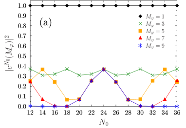
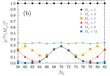
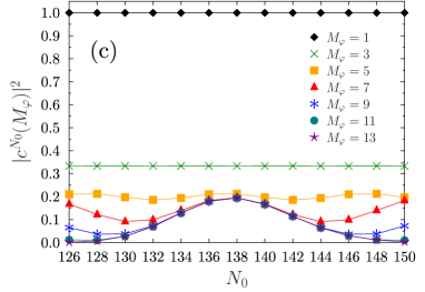
Figure 1: (Color online) Evolution of the weight $|c^{N_{0}}(M_{\varphi})|^{2}$ of the numerically projected states as a function of the number of neutrons $N_{0}$ on which one projects for different choices for the number of discretization points ${M_{\varphi}}$ for the quasiparticle states $|\Phi_{a}\rangle$ (panel (a)), $|\Phi_{b}\rangle$ (panel (b)) and $|\Phi_{c}\rangle$ (panel (c)) as specified in the text. On each panel, the results obtained with the largest value of ${M_{\varphi}}$ cannot be distinguished from exact results for the values of $N_{0}$ shown. Points calculated with same $M_{\varphi}$ are connected by straight lines to guide the eye.

To illustrate the further discussion of the convergence of results obtained with the discretized projection operator $\hat{\mathbb{P}}^{N_{0}}_{M_{\varphi}}$ (72) in dependence of the number of discretization points $M_{\varphi}$, we will examine the decomposition of three (normalized) fully paired Bogoliubov-type quasiparticle states $|\Phi\rangle$. The states were constructed for ⁴⁴Ca, ¹²⁰Sn and ²²⁰Pb. Also, the states were chosen such that their dispersion of neutron number

$$\langle\Phi|\Delta\hat{N}^{2}|\Phi\rangle\equiv\langle\Phi|\hat{N}^{2}|\Phi\rangle-\langle\Phi|\hat{N}|\Phi\rangle^{2}\,,$$ (73)

which provides a measure for the breaking of global gauge symmetry through the presence of pairing correlations, is increasing. The actual values for the mean neutron number $\langle\Phi|\hat{N}|\Phi\rangle$ and its dispersion are given in Tab. 1.

For our purpose it is sufficient to consider only projection on neutron number, while leaving the proton part of the wave function untouched.

In Fig. 1, we plot, for these three states, the weights of the numerically projected states

$$|c^{N_{0}}({M_{\varphi}})|^{2}=\langle\Phi|\hat{\mathbb{P}}^{N_{0}}_{M_{\varphi}}|\Phi\rangle$$ (74)

in dependence of the total number of discretization points $M_{\varphi}$. As already mentioned, for $M_{\varphi}=1$ the discretized projection operator (72) is the unit operator. This means that $\hat{\mathbb{P}}^{N_{0}}_{1}$ does not project at all and attributes the unaltered original state to any particle number $N_{0}$ compatible with that state’s number parity, independent of that component being contained in the state’s physical decomposition or not, cf. Fig. 1. From a different perspective, for $M_{\varphi}=1$ the discretized projection operator attributes the complete sum of all physical components $|\Psi^{N_{1}}\rangle$ with their physical weight $c^{N_{1}}=c^{N_{1}}(M_{\varphi}=\infty)$ to any particle number $N_{0}$ compatible with its number parity

$$\hat{\mathbb{P}}^{N_{0}}_{1}|\Phi\rangle=|\Phi\rangle=\sum_{N_{1}}c^{N_{1}}|\Psi^{N_{1}}\rangle\,.$$ (75)

Each of the thus numerically “projected” states is equal, and its observables take the value of the sum rule for projection, even when the respective component is absent from the original symmetry-breaking state.

These observations provide the starting point for the understanding of how the discretized projection operator (72) generates projected states for finite values of $M_{\varphi}$ by eliminating non-targeted components from the summation in Eq. (75). As demonstrated in Appendix A, for finite $M_{\varphi}>1$ applying the discretized projection operator $\hat{\mathbb{P}}^{N_{0}}_{M_{\varphi}}$ on a state removes exactly all components that do not satisfy the condition $N_{1}=N_{0}+2l{M_{\varphi}}$, $l\in\mathbb{Z}$, from the original state. The final result can be expressed in a compact way as the double sum

$$\hat{\mathbb{P}}^{N_{0}}_{M_{\varphi}}|\Phi\rangle=\sum_{l\in\mathbb{Z}}\sum_{N_{1}\geq 0}c^{N_{1}}|\Psi^{N_{1}}\rangle\,\delta_{N_{1}N_{0}+2lM_{\varphi}}\,.$$ (76)

The subset of non-targeted components contained in the original state that are not eliminated by the discretized projection operator quickly becomes smaller with increasing $M_{\varphi}$. For a given $N_{0}$, the closest non-suppressed components are the ones at $N_{0}\pm 2M_{\varphi}$.

In theory, the non-vanishing irreps $N_{0}$ contained in a Bogoliubov quasiparticle state $|\Phi\rangle$ will fall into an interval bounded by $N_{\text{min}}$ and $N_{\text{max}}$. The lower bound $N_{\text{min}}$ is given by the number of fully occupied single-particle states in the canonical basis of $|\Phi\rangle$ while the upper bound $N_{\text{max}}$ is given by the total number of single-particle states with non-zero occupation in the same basis. In practice, however, the wave function is generated numerically such that the bounds might be affected by the numerical accuracy of the computation, which is ultimately limited by floating-point arithmetic, and can only delimit an interval outside of which the respective components cannot be distinguished from numerical noise.

For a given irrep $N_{0}$ with non-zero weight, the discretized projection operator (72) becomes exact when all other components from $N_{\text{min}}$ to $N_{\text{max}}$ have been eliminated. For a given $M_{\varphi}$, the interval for which the discretized numerical projection on particle number $N_{0}$ (72) becomes exact is

$$N_{\text{max}}-2M_{\varphi}+2\leq N_{0}\leq N_{\text{min}}+2M_{\varphi}-2\,.$$ (77)

Nevertheless, if one has a prior knowledge of the distribution of the projected components, it is possible to adapt the discretization depending on the localization of the targeted irrep within the distribution. As it will be demonstrated later on, for Bogoliubov quasiparticle vacua one can assume up to a very good approximation a Gaussian shaped distribution centered around the average particle-number of the state, see the discussion of Eq. (79) in what follows. In that case, for $N_{0}$ next to the center of the distribution at $\big{(}N_{\text{min}}+N_{\text{max}}\big{)}/2\approx\langle\hat{N}\rangle$, this requires $M_{\varphi}>\big{(}N_{\text{max}}-N_{\text{min}}\big{)}/4\approx 1.5\,\langle\Delta\hat{N}^{2}\rangle^{1/2}$ points, where we used Eq. (79) for the estimate in terms of the dispersion in particle number (73). This represents the simplest case that sets the lower limit for an acceptable value of $M_{\varphi}$. On the other hand, for targeted irreps $N_{0}$ at the boundary of the interval, all other components are eliminated for $M_{\varphi}>\big{(}N_{\text{max}}-N_{\text{min}}\big{)}/2\approx 3\,\langle\Delta\hat{N}^{2}\rangle^{1/2}$, see Fig. 1.

For components $N_{0}$ absent from the original state, however, the convergence towards the correct result $c^{N_{0}}=0$ in general requires more integration points. Indeed, Eq. (76) implies that the discretized projection operator has a periodicity of $2M_{\varphi}$ and therefore yields the same numerical result for particle numbers $N_{0}$ that differ by multiples of $2M_{\varphi}$. As a consequence, it generates mirror images of the results for $N_{0}$ that are repeated every $2lM_{\varphi}$, as can be clearly seen in Fig. 1. A special case is $M_{\varphi}=1$, for which these mirror images superpose in such a way that the numerically “projected” state is the sum of all physical components for all values of $N_{0}$ permitted by number parity. When $M_{\varphi}>(N_{\text{max}}-N_{\text{min}})/2$, then some components outside of this interval are also correctly identified as having weight zero, but not all of them. A safe choice in that case would be to take $M_{\varphi}>|\big{(}N_{\text{max}}+N_{\text{min}}\big{)}/2-N_{0}|\approx|\langle\hat{N}\rangle-N_{0}|$, although fewer points may already be sufficient.

As the periodic mirror images of the dominant components are pushed away from the interval of physical components when increasing $M_{\varphi}$, the numerical results obtained for weights $|c^{N_{0}}(M_{\varphi})|^{2}$ of components $N_{0}$ far outside of the interval defined through Eq. (77) will oscillate between the values of various weights of physical components (or sums thereof) and zero, until they fall into the interval defined in Eq. (77). The effect can be seen for example in panel (a) of Fig. 1 for $|c^{14}|^{2}$ and $|c^{34}|^{2}$, which non-montonically jump around before falling to zero. For components much further outside, such oscillation will repeat itself several times with increasing $M_{\varphi}$.

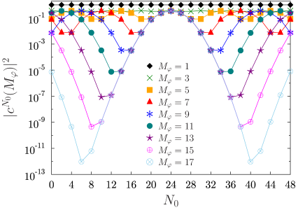
Figure 2: (Color online) Same as panel (a) of Fig. 1, but in logarithmic scale and some additional values of $M_{\varphi}$.

The queues of the distributions analyzed in Fig. 1 fall off relatively slowly, which can be more clearly seen when plotting the same data on a logarithmic scale as done for the decomposition of one of the states in Fig. 2. Still, the numerical convergence of these tiny components continues in the same way as the convergence of the dominant ones until a level of $10^{-13}$ has been reached, beyond which the numerical noise from the calculation of many-body matrix elements sets in in our code. This figure also shows even more clearly than Fig. 1 how the identical mirror images at $N_{0}+2M_{\varphi}$ of converged physical components at $N_{0}$ move outside with increasing $M_{\varphi}$ in the discretized projection operator.

Figure 3: (Color online) Deviation (78) in logarithmic scale of the sum rule for the components $|c^{N_{0}}(M_{\varphi})|^{2}$ of the state $|\Phi_{a}\rangle$ from the analytical value one as a function of $M_{\varphi}$. See text for details. to guide the eye.

The sum rule for the weights (28) establishes an additional test of the internal consistency and the numerical accuracy of the projection of a given state. Focusing on state $|\Phi_{a}\rangle$, we display in Fig. 3, the sum rule for the components $|c^{N_{0}}(M_{\varphi})|^{2}$ summed from $N_{0}=0$ to 48 and subtracted by one, i.e. the quantity

$$\Sigma(M_{\varphi})\equiv\left|\sum_{N_{0}=0}^{48}|c^{N_{0}}(M_{\varphi})|^{2}-1\right|\,,$$ (78)

as a function of $M_{\varphi}$.

As argued above, for $M_{\varphi}=1$, the numerical projection operator $\hat{\mathbb{P}}^{N_{0}}_{1}$ attributes the entire sumrule to any irrep $N_{0}$ compatible with the number parity of the original state (75). Calculating the sum rule in that case yields the mean-field expectation value of the operator in question times the number of irreps summed over. With increasing number of discretization points $M_{\varphi}$ in the numerical projector $\hat{\mathbb{P}}^{N_{0}}_{M_{\varphi}}$ (72), the non-physical contributions to the matrix element for $N_{0}$ are eliminated as a result of relation (76) until convergence to the physical value for the irrep $N_{0}$ is reached. For convergence of the sum rule, it is obviously necessary that the summation covers all irreps found in the original state $|\Phi_{a}\rangle$ and that the number of discretization point is sufficient to converge the calculation of the projected matrix elements.

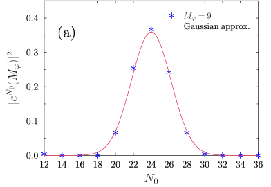
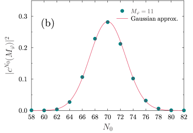
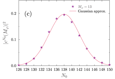
Figure 4: (Color online) Comparison between the weight $|c^{N_{0}}(M_{\varphi})|^{2}$ of the numerically projected states (markers) and its Gaussian approximation (79) (solid line) as a function of the number of neutrons $N_{0}$ on which one projects for the quasiparticle states $|\Phi_{a}\rangle$ (panel (a)), $|\Phi_{b}\rangle$ (panel (b)) and $|\Phi_{c}\rangle$ (panel (c)) as specified in the text. On each panel, the number of points ${M_{\varphi}}$ used is the same as the largest one displayed in Fig. 1.

To be sure about the numerical convergence of results without running test calculations with different values of $M_{\varphi}$ requires the a priori knowledge of the boundaries $N_{\text{max}}$ and $N_{\text{min}}$ of the distribution of irreps in the original state. As has been demonstrated in Ref. Flocard and Onishi (1997), the distribution of the weights (58) of components with particle number $N$ in the decomposition of a fully paired Bogoliubov quasiparticle state $|\Phi\rangle$ can be estimated by a Gaussian centered around its average particle number $\langle\Phi|\hat{N}|\Phi\rangle$

$$|c^{N_{0}}|^{2} \approx\frac{2}{\sqrt{2\pi\sigma^{2}}}\exp\bigg{[}-\frac{\big{(}\langle\Phi|\hat{N}|\Phi\rangle-N_{0}\big{)}^{2}}{2\sigma^{2}}\bigg{]}\,,$$ (79)

whose width is determined by that state’s dispersion of particle number: $\sigma^{2}=\langle\Phi|\Delta\hat{N}^{2}|\Phi\rangle$, see also Ref. Samyn et al. (2004).

For the fully paired quasiparticle vacua decomposed in Figs. 1, the exact values of the $|c^{N_{0}}|^{2}$ are indeed very well approximated by the Gaussian of Eq. (79), even for very small components as can be seen from Fig. 4. However, it should be noted that the presence of such small components far from the center of the distribution depends on choices made for cutoffs when solving the HFB equations. A cutoff that limits pairing correlations to some valence space will inevitably cut the tails from the distribution of irreps contained in the symmetry-breaking state. In any event, the remaining differences between the estimate and the calculated values are quite small, mainly in the form of a slight asymmetry around the center. The latter is not too surprising as the estimate (79) implies in one way or another equally distributed single-particle states and a state-independent pairing interaction, neither of which is the case in a realistic calculation. Nevertheless, the agreement is remarkable and the estimate (79) can hence be used to determine an a priori indication for the number of points ${M_{\varphi}}$ needed to converge the numerical projection, which in practice remains rather small ($M_{\varphi}\simeq 10$) for atomic nuclei.

It can be easily shown that for numerically projected matrix elements of any operator, for example a scalar operator $\hat{O}$, the elimination of untargeted components follows the same rule as for the plain norm overlap. Indeed, the normalized expectation value of such operator can be written as

$$\langle\hat{O}\rangle_{N_{0}}(M_{\varphi})\equiv\frac{\langle\Phi|\hat{O}\,\hat{\mathbb{P}}^{N_{0}}_{M_{\varphi}}|\Phi\rangle}{\langle\Phi|\hat{\mathbb{P}}^{N_{0}}_{M_{\varphi}}|\Phi\rangle}$$

$$=\frac{\sum_{\begin{subarray}{c}l_{1}\in\mathbb{Z}\\ N_{1}\geq 0\end{subarray}}|c^{N_{1}}|^{2}\,\langle\Psi^{N_{1}}|\hat{O}|\Psi^{N_{1}}\rangle\,\delta_{N_{1},N_{0}+2l_{1}{M_{\varphi}}}}{\sum_{\begin{subarray}{c}l_{2}\in\mathbb{Z}\\ N_{2}\geq 0\end{subarray}}|c^{N_{2}}|^{2}\,\delta_{N_{2},N_{0}+2l_{2}{M_{\varphi}}}}\,.$$ (80)

For $M_{\varphi}=1$, the normalized projected matrix element reduces to the plain expectation value $\langle\Phi|\hat{O}|\Phi\rangle$. Otherwise, for irreps with $|c^{N_{0}}|^{2}\neq 0$ in $|\Phi\rangle$, all other contributions but the targeted one have been eliminated in the numerator and the denominator when $M_{\varphi}$ is large enough that $N_{0}$ falls into the interval defined by Eq. (77). The rate of convergence, however, may depend also on the values of the exact projected matrix elements in the numerator.

Note that, while theoretically Eq. (III.6) can be written only for irreps $N_{0}$ with non-zero weights $|c^{N_{0}}|^{2}\neq 0$ in the original state, numerically neither the numerator nor the denominator will ever fully vanish, such that numerically one ends up with the division of numerical noise representing $\langle\Phi|\hat{O}\,\hat{\mathbb{P}}^{N_{0}}_{M_{\varphi}}|\Phi\rangle=0$ by different numerical noise representing $\langle\Phi|\hat{\mathbb{P}}^{N_{0}}_{M_{\varphi}}|\Phi\rangle=0$. This is an artifact of the numerical treatment of projection, as formally operators can have non-zero expectation values only for irreps with non-zero weights, cf. Eq. (47). For that reason, the expectation value of operators for small components $\langle\Phi|\hat{\mathbb{P}}^{N_{0}}_{M_{\varphi}}|\Phi\rangle$ have to be considered with care.

Figure 5: (Color online) Evolution of the deviation of the expectation value of the neutron number from the value it is projected on (a) and dispersion of the neutron number (b) for states numerically projected on particle number $N_{0}$ from the state with $\langle\Phi_{a}|\hat{N}|\Phi_{a}\rangle=24$ for the number of discretization points ${M_{\varphi}}$ as indicated. Points calculated with same $M_{\varphi}$ are connected by straight lines to guide the eye.

As an example for the numerical convergence of the matrix elements projected on irreps in the tails of the distribution, Fig. 5 displays the evolution of the deviation of the expectation value of the neutron number

$$\langle\hat{N}\rangle_{N_{0}}({M_{\varphi}})=\frac{\langle\Phi|\hat{N}\,\hat{\mathbb{P}}^{N_{0}}_{M_{\varphi}}|\Phi\rangle}{\langle\Phi|\hat{\mathbb{P}}^{N_{0}}_{M_{\varphi}}|\Phi\rangle}$$ (81)

from the value $N_{0}$ projected on, and also the dispersion

$$\langle\Delta\hat{N}^{2}\rangle_{N_{0}}({M_{\varphi}})=\langle\hat{N}^{2}\rangle_{N_{0}}({M_{\varphi}})-\langle\hat{N}\rangle^{2}_{N_{0}}({M_{\varphi}})\,,$$ (82)

in dependence of the number of discretization points ${M_{\varphi}}$ for a wide range of components projected from the state with $\langle\Phi_{a}|\hat{N}|\Phi_{a}\rangle=24$. Assuming again that the original state contains numerically significant irreps between $N_{\text{min}}\simeq 8$ and $N_{\text{max}}\simeq 40$, then Eq. (77) indicates that components can be expected to be converged for the maximum number of $M_{\varphi}=17$ points when they fall in the interval between about 8 and 40. In practice, however, for the very small components below $N_{0}\lesssim 12$ and above $N_{0}\gtrsim 32$, the precision of the numerical calculation of the matrix elements is visibly degraded compared to those in between. With our implementation that uses a double-precision floating-point format, further increasing the number of discretization points $M_{\varphi}$ does not significantly improve the quality of these components anymore.

Figure 6: (Color online) Evolution of the projected energy, for states with $N_{0}=24$, 70, and 138, projected from states with the same mean particle number as specified in Table 1, as a function of the total number of points ${M_{\varphi}}$ used for the discretized projection operator.

Another quantity that is sensitive to the number of particles is the projected binding energy

$$E^{N_{0}}({M_{\varphi}})=\frac{\langle\Phi|\hat{H}\,\hat{\mathbb{P}}^{N_{0}}_{M_{\varphi}}|\Phi\rangle}{\langle\Phi|\hat{\mathbb{P}}^{N_{0}}_{M_{\varphi}}|\Phi\rangle}\,.$$ (83)

As we are interested only in the accuracy of the discretized projection operator, neither the precise form of the Hamiltonian, nor the exact values of the energies are relevant, except that we specify that a true Hamiltonian is used when evaluating the projected energies in order to avoid any influence of the possible problems analyzed in Refs. Dönau (1998); Anguiano et al. (2001); Dobaczewski et al. (2007); Robledo (2007); Lacroix et al. (2009); Bender et al. (2009); Duguet et al. (2009); Robledo (2010); Satuła and Dobaczewski (2014) on our discussion. The results are displayed in Fig. 6 for projection of the three Bogoliubov quasiparticle vacua as specified in Table 1 on particle number $N=24$, 70, and 138, respectively As we can see, as we increase the number of points in the discretization, the energy converges rapidly. Beyond a certain value of $M_{\varphi}$, however, the numerical noise kicks in and increasing the number of points does not improve anymore the projected energy. It is also interesting to note that for the state $|\Phi_{a}\rangle$, the projected energy $E^{24}_{a}(M_{\varphi})$ is several hundreds of keV higher than the expectation value $\langle\Phi_{a}|\hat{H}|\Phi_{a}\rangle$ of the original state. Indeed, as previously explained in Sec. II.6, if the projection method guarantees to find at least one projected state of lower energy than the expectation value of the Hamiltonian of the original unprojected state, there is no reason that this will be the case for the irrep one is interested in. The latter depends both on the Hamiltonian at hand and how the unprojected state has been obtained.

Finally, we note in passing that particle-number-projected overlaps $\langle\Phi_{a}|\hat{\mathbb{P}}^{N_{0}}_{M_{\varphi}}|\Phi_{b}\rangle$ and non-diagonal matrix elements $\langle\Phi_{a}|\hat{O}\,\hat{\mathbb{P}}^{N_{0}}_{M_{\varphi}}|\Phi_{b}\rangle$ will converge with increasing $M_{\varphi}$ according to the values of $N_{\text{min}}$ and $N_{\text{max}}$ found in the two states. In the typical case where the distributions of components for $|\Phi_{a}\rangle$ and $|\Phi_{b}\rangle$ have a large overlap, the extremal values $\text{max}(N_{\text{min},a},N_{\text{min},b})$ and $\text{min}(N_{\text{max},a},N_{\text{max},b})$ will govern the convergence of the numerical projection. In more extreme cases, however, it is possible that the periodicity of the discretized projector induces contamination coming from distant, but physical, components.

IV Projection on angular momentum

IV.1 General Considerations

The second projection that we will analyze in detail is the projection on total angular momentum $J$. Together with proton number, neutron number, and parity, angular momentum is the most relevant quantum number for the analysis of spectroscopic data of atomic nuclei. As it provides selection rules for the existence of electromagnetic and other transitions and establishes rules for their relative strength, it provides the guideline to group states into characteristic level sequences Wigner (1959).

As explained in Sect. III.1, the angular-momentum projection of paired Bogoliubov-type quasiparticle vacua should be combined with particle-number projection. Angular-momentum projection is nowadays a widely employed technique in the context of nuclear EDF methods Bender et al. (2004a); Nikšić et al. (2006); Kimura (2007); Bender and Heenen (2008); Rodríguez and Egido (2010); Rodríguez-Guzman et al. (2012); Yao et al. (2011); Satuła et al. (2010); Bally et al. (2014); Borrajo et al. (2015); Rodríguez et al. (2015); Egido (2016); Egido et al. (2016); Robledo et al. (2018); Shimada et al. (2015); Ushitani et al. (2019); Bender et al. (2019). And angular-momentum projected quasiparticle vacua can also used as building blocks for configuration-interaction methods. Prominent examples are the MONSTER/VAMPIR approach Schmid and Grümmer (1987); Schmid (2004), the so-called projected shell model Hara and Sun (1995); Sun (2016) and the Monte-Carlo shell model Shimizu et al. (2012); Otsuka et al. (2001) that all present alternative numerical strategies to conventional shell-model calculations.

Only very few ground states of even-even nuclei will take the spherical symmetry of a $J=0$ state when calculated in a (symmetry-unrestricted) self-consistent mean-field approach. In fact, when calculated in HF approximation, only nuclei with subshells that are either completely filled or empty are even compatible with a strict spherical symmetry of the wave function.

Including pairing correlations in the modeling provides the means to describe spherical even-even open-shell systems with a single Bogoliubov quasiparticle vacuum, but such solutions are usually only found in the direct vicinity of major shell closures. Similarly, because of self-consistent core-polarization effects, it is virtually impossible that the variationally determined states for odd and odd-odd nuclei will be eigenstates of angular momentum.

Indeed, for the vast majority of nuclei, correlations related to the spatial arrangement of the nucleons are important. This is evidenced for example by the observation of collective rotational excitations that are an ubiquitous feature of nuclei throughout the chart of nuclei Bohr (1976); Rowe (1970); Bohr and Mottelson (1998); Ring and Schuck (1980); Frauendorf (2001), or by the evolution of charge radii that cannot be explained by consecutive filling of spherical shells with increasing nucleon number Angeli and Marinova (2015). To efficiently describe such correlations, it is advantageous to work with deformed reference states. Doing so, however, rotational symmetry is broken, and the resulting reference states are not eigenstates of angular momentum anymore. Angular momentum projection becomes mandatory to obtain a faithful and accurate description of related phenomena.

There is a noteworthy difference between the applications of angular-momentum and particle-number projection. In the literature, the latter is almost always exclusively used to extract one specific irrep from a symmetry-breaking state, which is very often the irrep with a particle number equal, or at least very close, to the one that the reference state has been constrained to, whereas angular-momentum projection in the majority of cases is used to project out a spectrum of states with different $J$. There are several reasons for this practice. The main reason is that nuclear structure changes often quickly with particle number, such that it is in most cases advantageous to construct reference states that are as close in particle number to the targeted one as possible. This is different for states with different angular momentum in a given nucleus: experiment indicates that they often have almost the same internal structure over a wide range of angular momenta, unless there is a backbending or other alignment phenomenon. And indeed, when being projected from a suitably chosen well-deformed quasiparticle vacuum, the angular-momentum restored states usually group into one or several rotational bands whose energies roughly scale with $J(J+1)$. Projecting on many irreps then even becomes a necessity for the interpretation of the internal structure of such symmetry-breaking state.

That collective rotational bands emerge naturally from an angular-momentum projected theory of quadrupole-deformed states can be shown analytically when expanding the Hamiltonian and norm kernels entering the projected energy in terms of rotation angles Peierls and Yoccoz (1957), thereby justifying phenomenological collective models for deformed nuclei Rowe (1970); Bohr and Mottelson (1998); Ring and Schuck (1980).

The same kind of expansion for well-deformed nuclei at high rotational frequency also yields the self-consistently cranked HF and HFB methods as a first-order limit Kamlah (1968); Beck et al. (1970); Villars and Schmeing-Rogerson (1971); Mang (1975); Wong (1975); Islam et al. (1979). In this approach, the energy is minimized with an auxiliary condition on the expectation value on a component of the angular momentum vector, where the rotational frequency plays the role of the Lagrange parameter, which leads to the so-called Thouless-Valatin moment of inertia Thouless and Valatin (1962).

There are several possibilities how to embed angular-momentum projection into a given framework. When the framework is variational, then VAP calculations are in general preferable over PAV, but they are computationally so costly that up to now such scheme has only been implemented for schematic bases Kanada-En’yo (1998) or small valence spaces Schmid and Grümmer (1987); Schmid (2004); Gao et al. (2015). Using a VAP scheme also has the drawback that in principle one has to do one such calculation for each value of $J$ of interest. The vast majority of applications uses the PAV scheme instead. There are, however, several strategies to arrive at an intermediate scheme in the spirit of an RVAP or MAP. As far as the optimal deformation of the state to be projected is concerned, one can construct a set of deformation-constrained states first that are then in a second step all projected on $J$ in order to identify the one given the lowest energy. This is particularly important for light nuclei in general and also nuclei with ground states at small deformation including spherical ones, for which the deformation of the reference state that gives the lowest projected states is usually very different from the deformation of the self-consistent ground state Bender et al. (2006). When combining angular-momentum projection with shape mixing in a GCM, such MAP is automatically done Bender et al. (2006). When projecting from the lowest variational state at a given deformation, such calculation is often characterized in terms of the Peierls-Yoccoz (or sometimes Yoccoz) moment of inertia Peierls and Yoccoz (1957) and systematically leads to excitation spectra that are slightly too spread out. This can be compensated for when working with states that are cranked to some rotational frequency, again either in a MAP scheme or by mixing states at different rotational frequency in a GCM. The latter strategy is characterized as using Peierls-Thouless moments of inertia Peierls and Thouless (1962). First applications along these lines using the Gogny EDF have recently become available Borrajo et al. (2015); Egido et al. (2016); Shimada et al. (2015); Ushitani et al. (2019)

We will now go into the details about the operation of projection on angular momentum. Neither for its formal aspects nor for the analysis of the convergence of the discretized projection operator is it of importance in which framework they are used. As above, for the sake of clarity we drop all symmetry indices not related to angular momentum throughout this section.

IV.2 Basic principles

The rotations in space of a single-particle state are characterized by the special unitary group $SU(2)$. Unlike global gauge rotations discussed above, $SU(2)$ is not Abelian. This will lead to a large number of formal and practical differences that make angular momentum projection more involved than particle-number projection.

The rotational invariance of the many-body Hamiltonian ensures that its eigenstates have good total angular momentum $J$. Contrarily to gauge invariance that is verified by protons and neutrons separately – and thus gives to two separate good quantum numbers $N$ and $Z$ – the rotational invariance is a property of the total wave function made by all the nucleons. Mathematically, this means that for a nucleus made of $A$ nucleons, the group of interest is the tensor product $\text{diag}(SU(2)\times\ldots\times SU(2))$, where the direct product contains $A$ times the group $SU(2)$. As $\text{diag}(SU(2)\times\ldots\times SU(2))$ is isomorphic to $SU(2)$, for the sake of simplicity we will simply label it as $SU(2)_{A}$. The irreps of $SU(2)_{A}$ are labeled by the angular momentum quantum number $J$ and have each a dimension $d_{J}=2J+1$. This means that, but for the trivial representation ($J=0$), the irreps of $SU(2)_{A}$ are not one dimensional as it was the case when dealing with the group $U(1)_{N}\times U(1)_{Z}$ for particle number. This is a consequence of the fact that the compact Lie group $SU(2)_{A}$ is not Abelian.

We choose to represent the unitary rotation operator $\hat{U}(g)$ of this group in terms of a sequence of three subsequent rotations about the $z$, $y$ and again the $z$ axis of a fixed coordinate system parameterized through the three Euler angles $(\alpha,\beta,\gamma)\in[0,2\pi]\times[0,\pi]\times[0,4\pi]$ Varshalovich et al. (1988)

$$\hat{R}(\alpha,\beta,\gamma)=e^{-\text{i}\alpha\hat{J}_{z}}\,e^{-\text{i}\beta\hat{J}_{y}}\,e^{-\text{i}\gamma\hat{J}_{z}}\,,$$ (84)

where $\hat{J}_{i}$ ($i=x,y,z$) is the component along the $i$-axis of the total angular momentum vector $\hat{\vec{J}}$. To lighten the notation, throughout this article we define the angular momentum operators without a factor $\hbar$. We note that there exist also alternative representations of the rotation operator that use a different sequences of rotations about different axes and angles Varshalovich et al. (1988).

As this will be of importance later on, we define next the three specific rotations of angle $\pi$ around each of the cartesian axis

$$\hat{R}_{x} =e^{-\text{i}\pi\hat{J_{x}}}=e^{-\text{i}\pi\hat{J_{y}}}\,e^{-\text{i}\pi\hat{J_{z}}}=\hat{R}(0,\pi,\pi)\,,$$ (85a)

$$\hat{R}_{y} =e^{-\text{i}\pi\hat{J_{y}}}=\hat{R}(0,\pi,0)\,,$$ (85b)

$$\hat{R}_{z} =e^{-\text{i}\pi\hat{J_{z}}}=\hat{R}(0,0,\pi)=\hat{R}(\pi,0,0)\,,$$ (85c)

with the operator $\hat{R}_{i}$ ($i=x,y,z$) being usually denoted as the $i$-signature in the nuclear physics literature Dobaczewski et al. (2000a).

In the parameterization of Eq. (84), the volume of the group is given by

$$v_{SU(2)_{A}}=\int_{0}^{2\pi}d\alpha\int_{0}^{\pi}d\beta\,\sin(\beta)\int_{0}^{4\pi}\!d\gamma=16\pi^{2}\,.$$ (86)

Its value being $16\pi^{2}$ is a consequence of looking at systems of Fermions, whose total wave functions can take integer or half integer total angular momenta. The different intervals covered by the Euler angles $\alpha$ and $\gamma$ can be interchanged without affecting the results.

The set of eigenstates $|\Psi^{JM}_{\epsilon}\rangle$ of $\hat{J}^{2}$ and $\hat{J}_{z}$

$$\hat{J}^{2}|\Psi^{JM}_{\epsilon}\rangle =J(J+1)|\Psi^{JM}_{\epsilon}\rangle\,,$$ (87)

$$\hat{J}_{z}|\Psi^{JM}_{\epsilon}\rangle =M|\Psi^{JM}_{\epsilon}\rangle\,,$$ (88)

and their respective quantum numbers $J$ and $-J\leq M\leq+J$ provide the basis functions and labels for the irreps of $SU(2)_{A}$. The generic label $\epsilon$ in (87) represents all additional characteristics of a state not directly affected by spatial rotations. Under such rotation, the basis functions transform as

$$\hat{R}(\alpha,\beta,\gamma)|\Psi^{JM}_{\epsilon}\rangle=\sum_{M^{\prime}=-J}^{J}D_{M^{\prime}M}^{J}(\alpha,\beta,\gamma)\,|\Psi^{JM^{\prime}}_{\epsilon}\rangle\,,$$ (89)

where the matrix representation $D_{M^{\prime}M}^{J}\,(\alpha,\beta,\gamma)$ of the group in the space of the rotation angles is provided by the Wigner rotation matrices Varshalovich et al. (1988)

$$\begin{split}D_{M^{\prime}M}^{J}(\alpha,\beta,\gamma)&=\delta_{J^{\prime}J}\,\langle\Psi^{J^{\prime}M^{\prime}}_{\epsilon}|\hat{R}(\alpha,\beta,\gamma)|\Psi^{JM}_{\epsilon}\rangle\\ &=e^{-\text{i}\alpha M^{\prime}}\,d_{M^{\prime}M}^{J}(\beta)\,e^{-\text{i}\gamma M}\end{split}$$ (90)

with $d_{M^{\prime}M}^{J}(\beta)$ being a Wigner $d$-matrix Varshalovich et al. (1988).

The operator that projects onto angular momentum $J$ for given $M$ and $K$ reads

$$\begin{split}\hat{P}^{J}_{MK}&=\frac{2J+1}{16\pi^{2}}\int_{0}^{2\pi}d\alpha\int_{0}^{\pi}d\beta\,\sin(\beta)\int_{0}^{4\pi}\!d\gamma\\ &\phantom{=}\times\,D_{MK}^{J*}(\alpha,\beta,\gamma)\,\hat{R}(\alpha,\beta,\gamma)\,,\end{split}$$ (91)

and has the properties

$$\hat{P}^{J}_{MK}\,\hat{P}^{J^{\prime}}_{M^{\prime}K^{\prime}} =\delta_{JJ^{\prime}}\,\delta_{KM^{\prime}}\,\hat{P}^{J}_{MK^{\prime}}\,,$$ (92)

$$\big{(}\hat{P}^{J}_{MK}\big{)}^{\dagger} =\hat{P}^{J}_{KM}\,.$$ (93)

These two equations indicate that for $M\neq K$ the operator $\hat{P}^{J}_{MK}$ is a transfer operator as defined in Sect. II, which is again a consequence of $SU(2)$ being non-Abelian.

While the integral representation (91) is the most transparent one from a group-theoretical point of view and the most flexible one as far as its combination with other symmetry restorations and configuration mixing is concerned, there are alternative representation of $\hat{P}^{J}_{MK}$ that have been sometimes used in specific contexts. One is in terms of angular-momentum shift operators Löwdin (1955), whose connection to the form (91) is sketched in Ref. MacDonald (1970). Another one that is based on direct diagonalization of angular momentum has been proposed in Ref. Morrison et al. (1974). More recently, the projection by solving a system of linear equations was also proposed Johnson and O’Mara (2017); Johnson and Jiao (2018). For a comparison of the computational cost of the various possibilities see for example Refs. MacDonald (1970); Kelemen and Dreizler (1975, 1976); Johnson and Jiao (2018).

Let us now consider the decomposition of a symmetry-breaking state $|\Phi\rangle$ into its content in orthogonal eigenstates of angular momentum. As explained in Sec. II, from very general properties of compact Lie groups it follows that the linear span $\text{span}(SU(2)_{A}|\Phi\rangle)$ constructed from all rotated states, i.e. the set $\big{\{}\hat{R}(\alpha,\beta,\gamma)|\Phi\rangle,\,(\alpha,\beta,\gamma)\in[0,2\pi]\times[0,\pi]\times[0,4\pi]\big{\}}$, can be decomposed as the direct sum of subspaces of dimension $d_{J}=2J+1$ that each carry an irrep $J$ of $SU(2)_{A}$

$$\text{span}(SU(2)_{A}|\Phi\rangle)=\bigoplus_{J}\bigoplus_{\epsilon=1}^{n_{J}}S^{J}_{\epsilon}\,.$$ (94)

The number $n_{J}$ of subspaces $S^{J}_{\epsilon}$ carrying the same irrep $J$ that can be found in the decomposition of $\text{span}(SU(2)_{A}|\Phi\rangle)$ depends on the structure of $|\Phi\rangle$, and we use the label $\epsilon$ to distinguish between them.

The natural way to obtain a full set of orthonormal basis states $\left\{|\Psi^{JM}_{\epsilon}\rangle,J,M\in\llbracket-J,J\rrbracket,\epsilon\in\llbracket 1,n_{J}\rrbracket\right\}$ withtin $\text{span}(SU(2)_{A}|\Phi\rangle)$ is to diagonalize the Hamiltonian within this space. To that end, in addition of the application of the operator it is necessary to solve the GEP

$$\boldsymbol{H}^{J}\boldsymbol{f}^{J}_{\epsilon}=e^{J}_{\epsilon}\boldsymbol{N}^{J}\boldsymbol{f}^{J}_{\epsilon}\,,$$ (95)

where $\boldsymbol{H}^{J}$ and $\boldsymbol{N}^{J}$ are the Hamiltonian and norm matrices, respectively, whose matrix elements are

$$H^{J}_{KK^{\prime}} =\langle\Phi|\hat{H}\hat{P}^{J}_{KK^{\prime}}|\Phi\rangle\,,$$ (96)

$$N^{J}_{KK^{\prime}} =\langle\Phi|\hat{P}^{J}_{KK^{\prime}}|\Phi\rangle\,.$$ (97)

At the end of the procedure, we end up with symmetry-restored states of the form

$$|\Psi^{JM}_{\epsilon}\rangle=\sum_{K=-J}^{J}f^{JK}_{\epsilon}\,\hat{P}^{J}_{MK}|\Phi\rangle\,,$$ (98)

that are, from a variational point of view, the optimal states with good angular momentum in the vector space $\text{span}(SU(2)_{A}|\Phi\rangle)$.

Expanding $|\Phi\rangle$ on these orthonormal basis states, we can write

$$|\Phi\rangle=\sum_{J}\sum_{\epsilon=1}^{n_{J}}\sum_{K=-J}^{J}c^{JK}_{\epsilon}|\Psi^{JK}_{\epsilon}\rangle\,,$$ (99)

with the normalization of $|\Phi\rangle$ leading to the sum rule

$$\begin{split}\langle\Phi|\Phi\rangle=1&=\sum_{J}\sum_{\epsilon=1}^{n_{J}}\sum_{K=-J}^{J}|c^{JK}_{\epsilon}|^{2}\\ &=\sum_{J}\sum_{K=-J}^{J}N^{J}_{KK}\,.\end{split}$$ (100)

This sum rule can be used to probe the numerical accuracy of the AMP and determine the appropriate number of points required to converge the discretized integral over Euler angles (see Sec. IV.5 for details) in numerical calculations. While both lines of Eq. (100) are equivalent, the second one has the practical advantage that it requires only the evaluation of projected matrix elements and not the precise determination of the weights

$$c^{JK}_{\epsilon}=\langle\Psi^{JK}_{\epsilon}|\Phi\rangle=\sum_{K^{\prime}=J}^{J}\big{(}f^{JK^{\prime}}_{\epsilon}\big{)}^{*}\,N^{J}_{K^{\prime}K}\,.$$ (101)

that can be done only after solving the GEP of Eq. (95). On the other hand, the advantage of calculating the coefficients $c^{JK}_{\epsilon}$ to make use of the first line of Eq. (100) is that it allows to check the numerical accuracy of the resolution of the GEP. In the end, both equalities can be used at the same time to test the numerical precision of at each step of the symmetry restoration.

It is interesting to remark that while the space $\text{span}(SU(2)_{A}|\Phi\rangle)$ contains for a given irrep all components $M\in\llbracket-J,J\rrbracket$, the decomposition (99) of the state $|\Phi\rangle$ may contain only part of them (but at least one). This is possible because $\text{span}(SU(2)_{A}|\Phi\rangle)$ is by design invariant under rotation, i.e. it is generated by rotating $|\Phi\rangle$ in every possible way, and therefore contains all the components $M$ of a given irrep, even those not present originally in the decomposition of $|\Phi\rangle$. For that reason, when discussing angular-momentum projection, one often uses a notation which distinguishes the angular-momentum components $K$ that a symmetry-breaking state $|\Phi\rangle$ can be decomposed into from the angular-momentum components $M$ that enter the calculation of the matrix elements of irreducible tensor operators between symmetry-restored states in the space $\text{span}(SU(2)_{A}|\Phi\rangle)$.

In the literature, the $K$ are sometimes associated with the $z$-component of angular momentum expressed in an “intrinsic” frame of reference, whereas $M$ labels angular momenta in the “laboratory” frame of reference. The notion of intrinsic and laboratory frame, however, has its ambiguities as it suggests that there are two different bases involved, one in an “intrinsic frame” attached to the nucleus as chosen by the theoretician when setting up the nucleus’ wave function and another one corresponding to what an experimentalist is observing in the laboratory. In the projection formalism described above, however, the $z$ direction that the such interpreted $K$ and $M$ refer to is the same, i.e. the basis states $|\Psi^{JM}_{\epsilon}\rangle$ are part of the same set of eigenstates of $\hat{J}_{z}$. The terminology of intrinsic and laboratory frame is in fact used by analogy with the Unified Model of Bohr and Mottelson and other collective models Bohr and Mottelson (1998); Rowe (1970); Ring and Schuck (1980), where the total wave function is assumed to be a factorization of an intrinsic part, which captures the internal structure of the nucleus, times a Wigner $D$-matrix that describes the orientation of the nucleus in the laboratory frame in terms of collective angular momentum degrees of freedom. In that case, the Wigner rotation matrix does indeed describe a transformation between two differently oriented frames of reference as mentioned above. The same relations are also used as an approximation when connecting self-consistent mean-field results for electric and magnetic moments with experimental data without symmetry restoration Siemens and Jensen (1987).

By contrast, within the projection method, the importance often given to the decomposition (99) into $K$-components of a state $|\Phi\rangle$ has to be tempered by the the fact that this decomposition depends on the orientation chosen to represent the state within the reference frame. As far as the projection method is concerned, this choice is completely arbitrary as from a formal point of view it has no effect on the final set of projected states $|\Psi^{JM}_{\epsilon}\rangle$. When the state to be projected has some intrinsic symmetries, as it is usually the case, some specific choices can be more advantageous than others from a computational point of view as they simplify the numerical construction of the reference state and the numerical solution of the GEP.

The more fundamental difference is between the states $\hat{P}^{J}_{MK}|\Phi\rangle$ simply obtained by the application of the projection operators and the states $|\Psi^{JM}_{\epsilon}\rangle$ that diagonalize the Hamiltonian in $\text{span}(SU(2)_{A}|\Phi\rangle)$. Indeed, the former keep a memory of the $K$-component they have been constructed from and therefore of the particular orientation chosen for $|\Phi\rangle$. By contrast, the latter (98) are constructed explicitly as a superposition of all $K$-components present in the decomposition of $|\Phi\rangle$ when diagonalizing the Hamiltonian, and as such they are independent of the initial orientation chosen for $|\Phi\rangle$. All states $|\Phi\rangle$ and $|\Phi^{\prime}\rangle=\hat{R}(\alpha,\beta,\gamma)|\Phi\rangle$ that differ only by a rotation will generate the same subspace $\text{span}(SU(2)_{A}|\Phi\rangle)$ and therefore the same symmetry-restored states after solving the GEP (95). Nevertheless, it is important to stress that wether we consider the states $\hat{P}^{J}_{MK}|\Phi\rangle$ or $|\Psi^{JM}_{\epsilon}\rangle$, the projection cannot be reduced to a mere change of reference frame. As a matter of fact, this interpretation would be contradictory to the fact that the Hamiltonian is rotationally invariant as it implies that one obtains different values for the energy in different reference frames.

IV.3 Distinguishing odd and even nuclei

We have seen in Sect. III.3 that Bogoliubov quasiparticle vacua $|\Phi\rangle$ are always eigenstates of a number parity operator (59), which permits to distinguish the states $|\Phi\rangle$ that only decompose on irreps with even particle number from those that decompose exclusively on irreps with odd particle number. The symmetry under this operator can then be used to reduce the integration interval for numerical particle number projection, provided that the number parity of a given Bogoliubov state is known a priori.

Given our choice of parametrization for the Euler angles, the operator that takes the same role for angular-momentum corresponds to a rotation about $2\pi$ around the $z$-axis

$$\hat{\Pi}_{J}=e^{-2\text{i}\pi\hat{J}_{z}}\,,$$ (102)

although, in practice any rotation about $2\pi$ around an arbitrary axis yields the same result. This operator is linked to the point-group operators discussed in Sect. V below by being equal to the square of any signature operator $\hat{\Pi}_{J}=\big{(}\hat{R}_{x}\big{)}^{2}=\big{(}\hat{R}_{y}\big{)}^{2}=\big{(}\hat{R}_{z}\big{)}^{2}$, which is why we will call it squared signature. Together with the usual binary operation, the set $\{\hat{{\mathchoice{\rm 1\mskip-4.0mul}{\rm 1\mskip-4.0mul}{\rm 1\mskip-4.5mul}{\rm 1\mskip-5.0mul}}},\hat{\Pi}_{J}\}$ defines a cyclic group of order two with two distinct irreps labeled by $\pi_{J}=\pm 1$, and which is a finite subgroup of $SU(2)_{A}$.

Because of the rules of angular-momentum coupling, the wave function of a system composed of an even number of fermions is such that $\pi_{J}=1$, whereas a state with an odd number of fermions has $\pi_{J}=-1$. This implies that for a fermionic wave function number parity and squared signature are equal

$$\pi_{J}=\pi_{n}\,.$$ (103)

As a consequence, the Bogoliubov quasiparticle state $|\Phi\rangle$, which is a superposition of projected states with either an even or an odd number of fermions, is such that

$$\hat{\Pi}_{J}|\Phi\rangle=\pi_{J}|\Phi\rangle\,.$$ (104)

which leads also to the equality

$$c^{JK}_{\epsilon}=\pi_{J}\,(-)^{2J}\,c^{JK}_{\epsilon}$$ (105)

for the weights $c^{JK}_{\epsilon}$ entering the decomposition (99).

As a result, a quasiparticle state with squared signature $\pi_{J}=+1$ is a superposition of basis states $|\Psi_{\epsilon}^{JK}\rangle$ with an integer angular momentum, whereas a quasiparticle state with $\pi_{J}=-1$ is a superposition of basis states with an half-integer angular momentum.

Analogously to the simplification of particle-number projection for states with good number parity, we can simplify angular-momentum projection for eigenstates of squared signature. Indeed, as can be easily shown, in this case the integration interval for the angle $\gamma$ in the projection operator can be reduced from $[0,4\pi]$ to $[0,2\pi]$ Bally (2014); Varshalovich et al. (1988), leading to the numerically less costly reduced projection operator

$$\begin{split}\hat{\mathcal{P}}^{J}_{MK}&=\frac{2J+1}{8\pi^{2}}\int_{0}^{2\pi}d\alpha\int_{0}^{\pi}d\beta\sin(\beta)\int_{0}^{2\pi}\!d\gamma\\ &\phantom{=}\times\>D_{MK}^{J*}(\alpha,\beta,\gamma)\,\hat{R}(\alpha,\beta,\gamma)\,.\end{split}$$ (106)

Its form is the same for both possible eigenvalues of squared signature. However, the reduced projection operator (106) cannot distinguish anymore between states having different eigenvalues of $\hat{\Pi}_{J}$. Indeed, the operator of Eq. (106) is now a projection operator for a specific class of states, where the irrep $J$ one projects out has to be chosen according to the squared signature of the states it acts on, i.e. $\pi_{J}=(-)^{2J}$.

IV.4 Evaluation of observables

A large number of the observables of interest in nuclear structure are either irreducible tensor operators with respect to $SU(2)_{A}$ or can be decomposed in terms of sums and/or products of such operators. This is in particular the case for the observables of interest in nuclear spectroscopy such as the energy, radii, or electromagnetic moments and transition moments.

Labeling generically $\hat{T}^{\lambda}_{m}$ an irreducible tensor of rank $\lambda$, with $m\in\llbracket-\lambda,\lambda\rrbracket$, for any angle $(\alpha,\beta,\gamma)$ we have the relation

$$\hat{R}(\alpha,\beta,\gamma)\,\hat{T}^{\lambda}_{m}\,\hat{R}^{\dagger}(\alpha,\beta,\gamma)=\sum_{m^{\prime}=-\lambda}^{\lambda}D^{\lambda}_{m^{\prime}m}(\alpha,\beta,\gamma)\,\hat{T}^{\lambda}_{m^{\prime}}\,.$$ (107)

In the case of a scalar operator $\hat{T}^{0}_{0}$, e.g. the energy or the charge radius, the above relation reduces to the simple commutation relation

$$\big{[}\hat{R}(\alpha,\beta,\gamma),\hat{T}^{0}_{0}\big{]}=0\,.$$ (108)

from which directly follows the commutation relation of the scalar operator with the projection operators

$$\forall J,\,\forall M,K\in\llbracket-J,J\rrbracket^{2}\,,\quad\big{[}\hat{P}^{J}_{MK},\hat{T}^{0}_{0}\big{]}=0\,.$$ (109)

From a practical point of view, relations (92) and (109) imply that the evaluation of projected matrix elements of scalar operators requires only one application of the projection operator, either on the bra on the ket, which substantially reduces the numerical cost. We have already used this relation above when discussing the derivation of the GEP (95).

For irreducible tensor operators of higher rank, the commutator $\big{[}\hat{P}^{J}_{MK},\hat{T}^{\lambda}_{m}\big{]}$ is non-zero, but can be evaluated using relation (107) and using the Clebsch-Gordan series for the product of two Wigner $D$ matrices Varshalovich et al. (1988). With this, one finds for the reduced matrix elements of the tensor operator $\hat{T}^{\lambda}_{m}$, as defined through the Wigner-Eckart theorem Blaizot and Tolénado (1997); Drake (2006), between two projected states

$$\begin{split}&\langle\Psi^{J^{\prime}}_{\epsilon^{\prime}}||\hat{T}^{\lambda}||\Psi^{J}_{\epsilon}\rangle=\sqrt{2J^{\prime}+1}\sum_{K^{\prime}=-J^{\prime}}^{J^{\prime}}\sum_{K=-J}^{J}\big{(}f^{J^{\prime}K^{\prime}}_{\epsilon^{\prime}}\big{)}^{*}\,f^{JK}_{\epsilon}\\ &\qquad\times\sum_{m=-\lambda}^{\lambda}\sum_{M=-J}^{J}\left(JM\lambda m|J^{\prime}K^{\prime}\right)\langle\Phi|\hat{T}^{\lambda}_{m}\hat{P}^{J}_{MK}|\Phi\rangle\,\end{split}$$ (110)

where the $\left(JM\lambda m|J^{\prime}K^{\prime}\right)$ are Clebsch-Gordan coefficients Varshalovich et al. (1988). The reduced matrix elements are independent of the $z$-component of the angular momenta of the bra and the ket. Matrix elements between specific states from the two irreps can then be obtained from

$$\langle\Psi^{J^{\prime}M^{\prime}}_{\epsilon^{\prime}}|\hat{T}^{\lambda}_{m}|\Psi^{JM}_{\epsilon}\rangle=\frac{\left(JM\lambda m|J^{\prime}M^{\prime}\right)}{\sqrt{2J^{\prime}+1}}\langle\Psi^{J^{\prime}}_{\epsilon^{\prime}}||\hat{T}^{\lambda}||\Psi^{J}_{\epsilon}\rangle\,.$$ (111)

Proceeding in such a way, one formally reduces the calculation of doubly-projected matrix elements $\langle\Phi|\hat{P}^{J^{\prime}}_{M^{\prime}K^{\prime}}\,\hat{T}^{\lambda}_{m}\,\hat{P}^{J}_{MK}|\Phi\rangle$ between all non-trivial combinations of $K$, $K^{\prime}$, $M$, $M^{\prime}$, and $m$ to the evaluation of singly-projected matrix elements $\langle\Phi|\hat{T}^{\lambda}_{m}\,\hat{P}^{J}_{MK}|\Phi\rangle$ between all combinations in the much smaller set of $K$, $M$, and $m$. This brings a substantial reduction of the numerical cost of the calculation. The state on which the projection operator acts can either be the bra or, as chosen here, the ket.

From a different perspective, it is the Clebsch-Gordan coefficient by which the projected matrix element $\langle\Phi|\hat{T}^{\lambda}_{m}\hat{P}^{J}_{MK}|\Phi\rangle$ is multiplied in Eq. (LABEL:eq:OPredu) that directly selects, through the orthogonality relation

$$\begin{split}\sum_{m=-\lambda}^{\lambda}\sum_{M=-J}^{J}&\left(JM\lambda m|J^{\prime}K^{\prime}\right)\,\left(JM\lambda m|J^{\prime\prime}K^{\prime\prime}\right)\\ &=\delta_{J^{\prime}J^{\prime\prime}}\,\delta_{K^{\prime}K^{\prime\prime}}\,,\end{split}$$ (112)

the projected angular momentum $J^{\prime}$ and component $K^{\prime}$ of the bra that gives a non-zero contribution to the reduced matrix element without the need to explicitly project it out.

The discussion above can be trivially generalized to the calculation of matrix elements between states $|\Psi^{J^{\prime}M^{\prime}}_{a\epsilon^{\prime}}\rangle$ and $|\Psi^{J^{\prime}M^{\prime}}_{b\epsilon}\rangle$ projected out from different reference states $|\Phi_{a}\rangle$ and $|\Phi_{b}\rangle$, respectively. In that context, and using that $\hat{T}^{\lambda\dagger}_{m}=(-1)^{m}\,\hat{T}^{\lambda}_{-m}$, one can derive an additional useful symmetry for the reduced matrix elements Suhonen (2007)

$$\langle\Psi^{J^{\prime}}_{a\epsilon^{\prime}}||\hat{T}^{\lambda}||\Psi^{J}_{b\epsilon}\rangle=(-1)^{J^{\prime}-J}\langle\Psi^{J}_{b\epsilon}||\hat{T}^{\lambda}||\Psi^{J^{\prime}}_{a\epsilon^{\prime}}\rangle^{*}\,.$$ (113)

This relation implies that having calculated the reduced matrix elements $\langle\Psi^{J^{\prime}}_{a\epsilon^{\prime}}||\hat{T}^{\lambda}||\Psi^{J}_{b\epsilon}\rangle$ for all relevant combinations of ($J$, $\epsilon$) and ($J^{\prime}$, $\epsilon^{\prime}$) for given $|\Phi_{a}\rangle$ and $|\Phi_{b}\rangle$ along the lines of Eq. (111), one can use relation (113) to reconstruct all required reduced matrix elements $\langle\Psi^{J}_{b\epsilon}||\hat{T}^{\lambda}||\Psi^{J^{\prime}}_{a\epsilon^{\prime}}\rangle$ without the need to numerically calculate matrix elements where the projection operator acts on $|\Phi_{a}\rangle$.

Examples of observables of interest whose operators cannot be written in terms of irreducible tensor operators are the spatial densities and transition densities between symmetry-restored states Yao et al. (2012, 2015). As a consequence, their calculation requires the projection (hence, rotation) of both states entering the matrix elements. There are, however, tricks to simplify the application of one of the rotation operators, see Yao et al. (2012, 2015). Note, however, that the resulting densities take the quantum numbers of the projected states for which they are calculated.

IV.5 Numerical implementation

For several reasons, the numerical evaluation of the angular-momentum projection of Bogoliubov-type quasiparticle vacua is much more involved than their particle-number projection. First, in the general case one has to deal with the evaluation of a three-dimensional integral over Euler angles instead of two separate one-dimensional integrals over proton and neutron gauge angles, respectively. Second, as it will be explained later on, the number of points required to accurately discretize each of the three integrals over Euler angles is usually larger than what is typically needed for gauge-space integrals as discussed in Sect. III.6, such that the total number of integrands to be evaluated can be several orders of magnitude larger. Also, unless when working in a spherical basis, which becomes problematic at large deformation, the numerical representation of rotation in space about the Euler angle $\beta$ always mixes all states of same parity in the single-particle basis with each other.

Nevertheless, each combination of angles $(\alpha,\beta,\gamma)$ being independent from the others, one deals with an embarrassingly parallel problem that can be parallelized with almost a perfect linear scaling. In addition, profiting from the structure of the integrands, it is possible to use efficient discretization of the three integrals.

As the integrals over $\alpha$ and $\gamma$ have a structure alike the one of the integral over gauge angles, we use for both of them a discretization similar to the one of Fomenko for particle-number projection (72)

$$\hat{\mathbb{P}}^{K_{0}}_{z,M_{\gamma}}=\frac{1}{M_{\gamma}}\,\sum_{n=1}^{M_{\gamma}}e^{-\text{i}2\pi\frac{n-\frac{1}{2}}{M_{\gamma}}(\hat{J}_{z}-K_{0})}\,,$$ (114)

explicated here for the angle $\gamma$. There are a few comments that we can make about the motivation of this choice

1. The use of a midpoint rule (114) instead of the repeated rectangular rule used to discretize the particle-number projection operator (72) will be of advantage for the efficient exploitation of symmetries of the integrand that result from intrinsic symmetries of the states to be projected and that will be discussed in Sect. V. As a consequence, however, the first point of the discretization is at $\frac{\pi}{M_{\gamma}}$ instead of zero. Therefore, the operator (114) does not reduce to the identity for $M_{\gamma}=1$, and the case of “no projection” has thus to be treated separately.

2. Note that because of the identical choice of quadrature for the integrals over $\alpha$ and $\gamma$, the action of the discretized projection operator is trivially symmetric under the exchange of the bra and ket as long as the same number of discretization points is used for both of these angles.

3. The operator $\hat{\mathbb{P}}^{K_{0}}_{z,M_{\gamma}}$ is a discretization of the reduced projection operator of Eq. (106). Therefore we can use $\hat{\mathbb{P}}^{K_{0}}_{z,M_{\gamma}}$ only to project states that have a squared signature equal to $(-)^{2K_{0}}$. A more general operator that works whatever the squared signature of the reference state, meaning that its application to a state with squared signature $\pi_{Ja}\neq(-)^{2K_{0}}$ yields matrix elements that are numerically zero, could be defined by replacing, either for $\alpha$ or $\gamma$, the factor $2\pi$ in the exponential by a factor $4\pi$. Like in the case of particle number projection, applying such operator would be twice as costly.

By applying the discretized operator $\hat{\mathbb{P}}^{K_{0}}_{z,M_{\gamma}}$ on a reference state $|\Phi_{a}\rangle$ with squared signature $\pi_{Ja}=(-)^{2K_{0}}$, we remove exactly all $K$ components such that $K_{1}\neq K_{0}+lM_{\gamma}$, $l\in\mathbb{Z}$ from the wave function

$$\hat{\mathbb{P}}^{K_{0}}_{z,M_{\gamma}}|\Phi_{a}\rangle=\sum_{J_{1}}\sum_{\epsilon=1}^{n_{J_{1}}}\sum_{l\in\mathbb{Z}}(-)^{l}\,c^{J_{1}K_{0}+lM_{\gamma}}_{a\epsilon}|\Psi^{J_{1}K_{0}+lM_{\gamma}}_{a\epsilon}\rangle\,.$$ (115)

Unfortunately, there is no discretization for the integral over $\beta$ that would lead to a similar removal of directly identifiable $J$ components from the non-projected state. But the structure of the volume element suggests to use a $M_{\beta}$-point Gauss-Legendre quadrature rule

$$\hat{\mathbb{P}}^{J_{0}M_{0}K_{0}}_{y,M_{\beta}}=\frac{2J_{0}+1}{2}\sum_{i=1}^{M_{\beta}}\,\omega_{i}\,d_{M_{0}K_{0}}^{J_{0}}(\beta_{i})\,e^{-\text{i}\beta_{i}\hat{J}_{y}}\,,$$ (116)

where $\beta_{i}=\arccos(x_{i})$, $x_{i}$ being the abscissa and $w_{i}$ the weight of the $i$-th point in the quadrature. One of the advantageous features of this quadrature is that it is exact for any polynomial in $x=\cos(\beta)$ that has an order lower or equal to $(2M_{\beta}-1)$. Given that the transformation of a state $|\Psi^{J_{1}K_{0}}_{a\epsilon}\rangle$ under rotation involves Wigner $d$-matrices of rank $J_{1}$, Eqs. (99), (89), and (90) imply that each component $J_{1}$ present in the state $|\Phi_{a}\rangle$ contributes as a polynomial of order $(J_{1}+J_{0})$ in $\cos(\beta)$ to the expectation value $d_{M_{0}K_{0}}^{J_{0}}(\beta_{i})\,\langle\Phi_{a}|e^{-\text{i}\beta_{i}\hat{J}_{y}}|\Phi_{a}\rangle$ of the l.h.s. of Eq. (116). Gauss-Legendre quadrature of the integral over this polynomial becomes exact if $M_{\beta}\geq(J_{0}+J_{1}+1)/2$. This means that when dealing with a wave function $|\Phi_{a}\rangle$ that is a superposition of irreps up to some $J_{\text{max}}$, the projection of the component with $J_{0}$ using $\hat{\mathbb{P}}^{J_{0}M_{0}K_{0}}_{y,M_{\beta}}$ becomes formally exact for

$$M_{\beta}\geq\frac{J_{0}+J_{\text{max}}+1}{2}\,.$$ (117)

Depending on the weight of the highest $J$ components in the state $|\Phi_{a}\rangle$, smaller values of $M_{\beta}$ might well be sufficient to calculate projected matrix elements with a numerically acceptable precision.

The full discretized projection operator on angular momentum thus reads

$$\hat{\mathscr{P}}^{J_{0}M_{0}K_{0}}_{M_{\alpha}M_{\beta}M_{\gamma}}=\hat{\mathbb{P}}^{M_{0}}_{z,M_{\alpha}}\,\hat{\mathbb{P}}^{J_{0}M_{0}K_{0}}_{y,M_{\beta}}\,\hat{\mathbb{P}}^{K_{0}}_{z,M_{\gamma}}\,,$$ (118)

with $M_{\alpha}$ points for $\alpha$, $M_{\beta}$ points for $\beta$, and $M_{\gamma}$ points for $\gamma$. Note first that, as the rotations around axes $z$ and $y$ do not commute it is not possible to change the order in which the discretized projection operators are applied on a state. Also, it is important to remark that because the orthogonality relation between two Wigner $d$-matrices is realized only for matrix elements of the same row ($M_{0}$) and column ($K_{0}$) Varshalovich et al. (1988), the accuracy of the operator that involves rotations around the $y$ axis by $\beta$, and which is always applied as the second one, is directly impacted by the accuracy of the operators acting on $\alpha$ and $\gamma$. An accurate numerical projection thus requires the simultaneous convergence of the three parts of the operator $\hat{\mathscr{P}}^{J_{0}M_{0}K_{0}}_{M_{\alpha}M_{\beta}M_{\gamma}}$.

Eventually, considering a number of points $M_{\alpha}$, $M_{\beta}$, $M_{\gamma}$ large enough, the full discretized projection operator will select only the desired component out of the reference state $|\Phi_{a}\rangle$, i.e.

$$\hat{\mathscr{P}}^{J_{0}M_{0}K_{0}}_{M_{\alpha}M_{\beta}M_{\gamma}}|\Phi_{a}\rangle\>\underset{M_{\alpha},M_{\beta},M_{\gamma}\to\infty}{\xrightarrow{\hskip 39.83368pt}}\>\sum_{\epsilon=1}^{n_{J_{0}}}c^{J_{0}K_{0}}_{a\epsilon}|\Psi^{J_{0}M_{0}}_{\epsilon a}\rangle\,.$$ (119)

To illustrate our discussion on the behavior of the discretized projection operators, we will study the numerical convergence of the angular-momentum projection of several Slater determinants constructed in the $sd$-shell valence space using the numerical suite TAURUS Bally et al. (2020, 2019). The use of Slater determinants for such analysis has the advantage that no particle-number projection is required, thus simplifying the calculations and removing a source of numerical inaccuracies (in particular as different $[N,Z]$ components will in general have different angular-momentum decompositions). Similarly, the $sd$-shell being solely made of positive parity single-particle states, the Slater determinants are automatically eigenstates of parity with eigenvalue $+1$. Performing the calculations with only a few particles in a restricted model space further simplifies the calculations, reduces the numerical noise (in particular as rotations are more accurately represented in a spherical harmonic oscillator basis than on a coordinate-space mesh) and provides a natural cutoff for the highest angular momentum than can appear in the decomposition of a given state.

To start with, we consider four Slater determinants built in the $sd$-shell using the USDB interaction Brown and Richter (2006). The states were obtained each starting from a randomly-generated and symmetry-unrestricted seed wave function but were constrained to have a certain value of the triaxial parameters $(\beta,\gamma)$. Their main characteristics are summarized in Tab. 2. To cover all cases of major interest, we consider for states for even-even [case (a) and (c)] and odd [case (b) and (b)] systems that at convergence either adopt an axial [cases (c) and (d)] or non-axial [case (a) and (b)] shape. We have to stress, however, that in a fully symmetry-unrestricted code the symmetries adopted by the self-consistent solutions are never perfect, such that there might also appear tiny contributions in the decomposition that result from the slight breaking of these intrinsic symmetries.

Label	$Z_{\text{val}}$	$N_{\text{val}}$	$(\beta,\gamma)$	$\langle\hat{J}_{z}\rangle$	$\langle\hat{J}^{2}\rangle$	$P$	$T$
a	2	2	$(0.075,30^{\circ})$	0	20	$+$	$+$
b	1	2	$(0.025,30^{\circ})$	-2.58	26.2	$+$	$-$
c	2	2	$(0.130,0^{\circ})$	0	16.1	$+$	$+$
d	2	3	$(0.130,0^{\circ})$	1.5	18.9	$+$	$-$

Table 2: Characteristics of the four Bogoliubov quasiparticle states considered for the convergence analyses displayed in Figs. 7, 8, 9, and 10 (see text). The values of $Z_{\text{val}}$ and $N_{\text{val}}$ indicate the number of valence protons and neutrons, respectively, whereas $\beta$ and $\gamma$ indicate the intrinsic quadrupole deformation. Finally, $\langle\hat{J}_{z}\rangle$ and $\langle\hat{J}^{2}\rangle$ denote the mean values of the angular-momentum operators as indicated. The columns $P$ and $T$ indicate if the symmetry-unrestricted self-consistent procedure converged towards a state that adopted the symmetry to be even or odd under space inversion and time reversal, either exactly or to a good numerical approximation, respectively (see text).

To investigate the projection on the third-component of the angular momentum, in Fig. 7 we plot the sum of $J_{0}$-components for a given $K_{0}$, i.e.

$$\Xi_{K_{0}}(M_{\alpha}\times M_{\beta}\times M_{\gamma})=\sum_{J_{0}}\langle\Phi|\hat{\mathscr{P}}^{J_{0}K_{0}K_{0}}_{M_{\alpha}M_{\beta}M_{\gamma}}|\Phi\rangle\,,$$ (120)

for different choices for the number of discretization points $M_{\alpha}=M_{\gamma}$, while we fix a large value of $M_{\beta}=20$. As will be shown later on, with the latter choice, we can assume that the numerical evaluation of $\hat{\mathbb{P}}^{J_{0}M_{0}K_{0}}_{y,M_{\beta}}$ is converged for the states considered for our analysis.

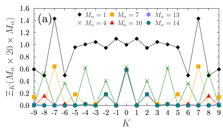
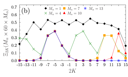
Figure 7: (Color online) Evolution of $\Xi_{K}(M_{\alpha}\times M_{\beta}\times M_{\gamma})$ as a function of the value of $K$ on which one projects for different choices for the number of discretization points $M_{\alpha}=M_{\gamma}$ for the quasiparticle states $|\Phi_{a}\rangle$ (panel (a)), $|\Phi_{b}\rangle$ (panel (b)), as specified in Table 2. Points calculated with same $M_{\alpha}=M_{\gamma}$ are connected by straight lines to guide the eye. On each panel, the results obtained with the largest value of $M_{\alpha}=M_{\gamma}$ cannot be distinguished from exact results for the values of $J_{0}$ shown.

We first notice that the two decompositions converge towards the physical values as one increases the number of discretization points in a manner that is very similar to what we observed for the projection on particle number in Sect. III.6. In particular, the discretized projection operator creates mirror images that are more and more pushed away to higher angular momenta until only the true distribution remains. Nevertheless, there are some key differences with the particle-number case. First of all, here the copies appear with the smaller periodicity $M_{\alpha}$ (instead of $2M_{\phi}$), which is to be expected given the factor $2\pi$ (instead of $\pi$) in the discretized operator of Eq. (114). Also, the mirror images are not perfect copies of each other but present some noticeable asymmetries. As pointed out above, an imperfect projection on $M_{0}$ or $K_{0}$ will spoil the application of the intermediate operator $\hat{\mathbb{P}}^{J_{0}M_{0}K_{0}}_{y,M_{\beta}}$ that is in between the two others, which might be the cause of those differences.

It is also interesting to remark that the two states display very different decompositions. The even-even state $|\Phi_{a}\rangle$ has a perfectly symmetric decomposition centered around $K_{0}=0$ and with only even values of $K_{0}$. On the other hand, the odd-even state $|\Phi_{b}\rangle$ has non-vanishing components only for negative values of $K_{0}$ but do not display any selection rules for the values of $K_{0}$. Typically, the distribution in terms of $K$ can be very different depending on the nature of the unprojected state (even or odd system, degree of non-axiality, etc) and the orientation of its major axes and therefore, contrarily to the particle-number case, there is no simple relation that could help us determine the minimal number of points sufficient to project out the targeted states with a good accuracy. However, symmetries of the unprojected many-body states, either imposed on them or adopted by them when solving the self-consistent HFB equations, will affect the components that can exist in their decompositions, as we will discuss in the Sec. V.

Another complication comes from the fact that an accurate projection of all $K_{0}$-components for a given $J_{0}$ is necessary to perform the subsequent mixing of $K$-components, which is necessary to fully diagonalize the Hamiltonian in the subspace of the projected states $\big{\{}\hat{P}^{J_{0}}_{MK}|\Phi\rangle\big{\}}$, Eq. (95). This fact tends to increase the number of discretization points required compared to the particle-number projection as this means that one needs to use enough points to converge even the extreme values of $K_{0}$ at the tail of the distribution. In the valence-space calculations employed here to illustrate convergence, however, we can easily calculate the extremal values that $K_{0}$ can take and that are $\pm 8$ for state $|\Phi_{a}\rangle$ and $\pm 13/2$ for state $|\Phi_{b}\rangle$. When the number of discretiztion points is insufficient, however, we can see that even higher values of $K_{0}$ numerically give non-vanishing results as they are part of mirror images of the physical distribution.

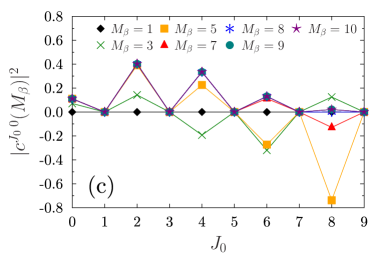
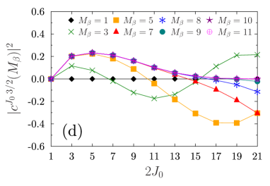
Figure 8: (Color online) Evolution of the weight $|c^{J_{0}K_{0}}(M_{\beta})|^{2}$ of the numerically projected states as a function of the angular momentum $J_{0}$ on which one projects for different choices for the number of discretization points $M_{\beta}$ for the quasiparticle states $|\Phi_{c}\rangle$ (panel (c)), $|\Phi_{d}\rangle$ (panel (d)), as specified in Table 2. Points calculated with same $M_{\beta}$ are connected by straight lines to guide the eye. On each panel, the results obtained with the largest value of ${M_{\beta}}$ is the first one for which the projection is exact for all values of $J_{0}$ plotted.

As mentioned before, the operator $\hat{\mathbb{P}}^{J_{0}M_{0}K_{0}}_{y,M_{\beta}}$ has a different numerical structure than the other two that enter the full discretized projection operator of Eq. (118) and that behave very similar to the discretized particle-number operator. To analyze the convergence of the operator $\hat{\mathbb{P}}^{J_{0}M_{0}K_{0}}_{y,M_{\beta}}$ more specifically, we consider now the two states $|\Phi_{c}\rangle$ and $|\Phi_{d}\rangle$ as specified in Tabke 2 that adopted axial symmetry and therefore can be treated as eigenstates of $\hat{J}_{z}$ with eigenvalue $K$, such that only the integral over $\beta$ has to be calculated numerically. In Fig. 8, we display the of weight of the projected component $K_{0}$

$$|c^{J_{0}K_{0}}(M_{\beta})|^{2}=\langle\Phi|\hat{\mathbb{P}}^{J_{0}K_{0}K_{0}}_{y,M_{\beta}}|\Phi\rangle\,,$$ (121)

for different choices for the number of discretization points $M_{\beta}$. Analogously to what is observed in Fig. 7, the discretized projection operator converges progressively as one increases the number of discretization points. The convergence pattern is, however, quite different. For a given value of $M_{\beta}$, one observes an oscillatory behavior as a function of $J_{0}$ that numerically can even take negative values whereas the exact projected weights $|c^{J_{0}K_{0}}|^{2}$ considered here are necessarily a positive quantity that can only take values between zero and one. When increasing the number of discretization points $M_{\beta}$, the oscillatory behavior of the distribution of the $|c^{J_{0}K_{0}}(M_{\beta})|^{2}$ disappears and converges towards the physical values for the weights.

Again, we remark that the distributions of the weights of the irreps that can be projected out from the two states $|\Phi_{c}\rangle$ and $|\Phi_{d}\rangle$ are very different. The even-even state $|\Phi_{c}\rangle$ contains only even values $J_{0}$ and the projection vanishes identically for odd values of $J_{0}$ for all values of $M_{\beta}$, even the smallest ones. That the state $|\Phi_{c}\rangle$ can only be decomposed onto irreps with even $J_{0}$ follows from the relations for the decomposition of states with intrinsic symmetries that will be elaborated in Sect. V, and is a consequence of this state having positive parity by construction and taking an axial shape. As the Wigner matrices $d^{J}_{00}(\cos(\beta))$ are even (odd) functions of $\cos(\beta)$ for even (odd) values of $J$, the kernel $\langle\Phi_{c}|\hat{R}_{y}(0,\beta,0)|\Phi_{c}\rangle$ of an axial state whose physical decomposition only contains even values of $J$ will also be an even function of $\cos(\beta)$. When choosing a discretization of $\cos(\beta)$ that is symmetric around zero as done with Eq. (116), then the numerical integrals over such kernel times an odd Wigner matrix $d^{J}_{00}(\cos(\beta))$ are automatically zero, irrespective of the number of discretization points $M_{\beta}$. Such selection rule is specific to $K=0$ states and has no analogue for the state $|\Phi_{d}\rangle$ that has $K=3/2$. For the latter, the only component that necessarily has to vanish is $J_{0}=1/2$, which numerically is achieved already for small values of $M_{\beta}$.

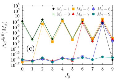
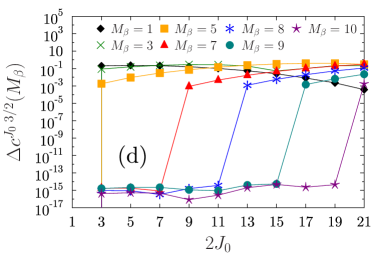
Figure 9: (Color online) Evolution of the difference between the numerical values for the weight $|c^{J_{0}K_{0}}(M_{\beta})|^{2}$ at $M_{\beta}$ as indicated and the converged values $|c^{J_{0}K_{0}}(M^{c}_{\beta})|^{2}$ obtained with $M^{c}_{\beta}=11$ in logarithmic scale as a function of angular momentum $J_{0}$ on which one projects for the quasiparticle states $|\Phi_{c}\rangle$ (panel (c)), $|\Phi_{d}\rangle$ (panel (d)), as specified in Table 2. Points calculated with same $M_{\beta}$ are connected by straight lines to guide the eye.

Given that the state $|\Phi_{c}\rangle$ is made of two neutrons and two protons in the $sd$-shell, the largest possible value of $J_{0}$ is 8, which is also what is found at convergence in the numerical decomposition. Having an additional neutron, the state $|\Phi_{d}\rangle$ can contain components having up to $J_{0}=19/2$. In this case, only $M_{\beta}=11$ reproduces exactly this result.

The convergence pattern explicated in Eq. (117) can be more explicitly seen in Fig. 9, where we display (in logarithmic scale) the same projected weights but subtracted from the converged values obtained with the discretization $M^{c}_{\beta}$, which is equal to the largest value of $M_{\beta}$ used in each panel of Fig. 8, i.e.

$$\Delta c^{J_{0}K_{0}}(M_{\beta})=\left|\langle\Phi|\hat{\mathbb{P}}^{J_{0}K_{0}K_{0}}_{y,M_{\beta}}|\Phi\rangle-\langle\Phi|\hat{\mathbb{P}}^{J_{0}K_{0}K_{0}}_{y,M^{c}_{\beta}}|\Phi\rangle\right|\,.$$ (122)

For example, in panel (d), the discretization $M_{\beta}=8$ gives exact results for components up to $J_{0}=11/2$: the difference to the converged value obtained with $M^{c}_{\beta}=11$ is of the order of the numerical noise. This can be easily understood using Eq. (117) as the largest physical value of $J_{1}$ in the distribution is $19/2$ and therefore $11/4+19/4+1/2=8$. Note that this rule applies even if the value $J_{0}$ onto which one projects is not in the distribution of components contained in the state to be projected. Indeed, $M_{\beta}=11$ is required to get the appropriate vanishing result for $J_{0}=21/2$, a component that cannot be contained in the Slater determinant $|\Phi_{d}\rangle$.

We note that the components with odd $J_{0}$ are not exactly zero on panel (c). This is a consequence of the state $|\Phi_{c}\rangle$ not having adopted a perfectly axially-symmetric shape when stopping the HFB iterations in the symmetry-unrestricted code. Even though the $\Delta c^{J_{0}K_{0}}(M_{\beta})$ are all tiny for odd values of $J_{0}$, at small values of $M_{\beta}$ they are nevertheless approximately eight order of magnitudes larger than the fully converged results.

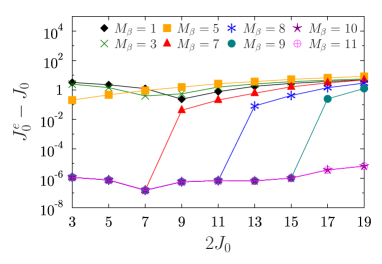
Figure 10: (Color online) Evolution in logarithmic scale of the difference $J_{0}^{e}-J_{0}$, where $J_{0}^{e}$ is extracted from Eq. (123), for the state $|\Phi_{d}\rangle$ as a function of the angular momentum $J_{0}$ onto which one projects for different choices for the number of discretization points $M_{\beta}$. Points calculated with same $M_{\beta}$ are connected by straight lines to guide the eye.

Finally, in Fig. 10 we plot, for the state $|\Phi_{d}\rangle$, the difference between the value of angular momentum $J_{0}^{e}$ extracted from the numerically projected matrix elements of $\hat{J^{2}}$ through the equation

$$\langle\Phi|\hat{J^{2}}\,\hat{\mathbb{P}}^{J_{0}K_{0}K_{0}}_{y,M_{\beta}}|\Phi\rangle=J_{0}^{e}(J_{0}^{e}+1)$$ (123)

and the targeted value $J_{0}$ as put into the projection operator. As one can see, the convergence of $J_{0}^{e}$ follows the same pattern as for the overlap. At the same discretization of the projection operator, however, the numerical accuracy of $J_{0}$ value of is general inferior.

The possible maximal angular momentum, and thereby the possible maximal width of the distribution of angular-momentum components, increases with the number of active particles in the model space. As a consequence, the angular-momentum projection of a state represented in the full space of occupied single-particle states can become much costlier than projecting a state represented in a small valence space not only because of the larger size of the single-particle basis, but also because of the larger number of discretization points that is needed for the projection operator.

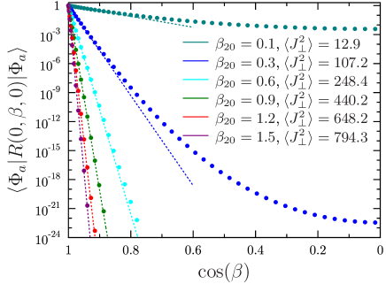
Figure 11: (Color online) Norm kernel as a function of the Euler angle $\beta$ on a logarithmic scale for axial reflection-symmetric states of ²⁴⁰Pu with dimensionless quadrupole moment $\beta_{20}$ and dispersion of angular momentum $\langle\Phi_{a}|\hat{J}^{2}_{\perp}|\Phi_{a}\rangle$ perpendicular to the symmetry axis as indicated. Dots indicate calculated values for the kernel using $M_{\beta}=96$ points, whereas the dotted lines represent the estimate defined in Eq. (124). For axial reflection-symmetric states, the norm kernel is a symmetric function around $\beta=\pi/2$ $\Leftrightarrow$ $\cos(\beta)=0$, $\langle\Phi_{a}|\hat{R}(0,\beta,0)|\Phi_{a}\rangle=\langle\Phi_{a}|\hat{R}(0,\pi-\beta,0)|\Phi_{a}\rangle$, cf. Eqns. (132b) and (132c), such that only half the integration interval for $\beta$ is shown.

As a rule of thumb, in a given model space the distribution of components contained in a state stretches further out with increasing deformation and increasing collective angular momentum Grümmer et al. (1978), thereby requiring an increasing number of discretization points for $\hat{\mathbb{P}}^{J_{0}K_{0}K_{0}}_{y,M_{\beta}}$ that are needed to attain the same level of convergence for a component with given $J_{0}$. This, however, is partially counterbalanced by the norm and operator kernels becoming increasingly sharply peaked as a function of $\beta$ Bender et al. (2006), such that the kernels might not have to be numerically evaluated for all combinations of Euler angles in the discretized projection operator. For the sake of clarity, we will exemplify this for the simple case of axial and reflection-symmetric time-reversal-invariant quasiparticle vacua of ²⁴⁰Pu calculated with a Skyrme EDF in a space that comprises all single-particle states with non-zero occupation. We choose states with a dimensionless prolate quadrupole moment of $\beta_{20}=0.1$, 0.3, 0.6, 0.9, 1.2 and 1.5. The state at 0.3 is close to the normal-deformed ground state, the state at 0.6 in the region of the inner fission barrier (whose saddle point corresponds to a non-axial state not considered here), the state at 0.9 close to the deformation of the excited superdeformed fission isomer, and the states at 1.2 and 1.5 in the outer barrier (whose actual saddle point corresponds to a non-axial reflection-asymmetric state not considered here).

To focus on angular-momentum projection, the states $|\Phi_{a}\rangle$ used to prepare Figs. 11 and 12 are normalized particle-number projected quasiparticle vacua. Recalling that the weights $\big{|}c^{J_{0}K_{0}}\big{|}^{2}$ of the numerically projected components are the sum over the product of the norm kernel $\langle\Phi_{a}|\hat{R}(\alpha,\beta,\gamma)|\Phi_{a}\rangle$ times a factor that is at most on the order one, it follows immediately that in a numerical representation that uses double-precision floating point arithmetic that Euler angles for which of the norm kernel between normalized states is smaller than $10^{-16}$ cannot meaningfully contribute to the sum. As the level of numerical noise is usually at a larger level, the limit for significant contributions can already be drawn at about $10^{-10}$.

Figure 11 shows the norm kernel as a function of the Euler angle $\beta$ for these states. For the smallest deformation, $\beta_{20}=0.1$, all Euler angles $\beta$ contribute significantly to the projected matrix elements. But already at the typical ground-state deformation of heavy nuclei $\beta_{20}\simeq 0.3$, the norm kernel falls off to values much smaller than $10^{-10}$ over a wide range of Euler angles, such that only those with $|\cos(\beta)|\gtrsim 0.7$ will contribute to the projected matrix elements. With increasing deformation the peak of the norm kernel narrows further, which reflects that for simply geometrical reasons an ever increasing part of the wave function that is at the tip of an elongated shape is rotated outside of the nucleus. This behavior of the norm kernel indicates that there is an additional condition for the numerical convergence of angular momentum projection: there has to be a sufficient number of integration points in the region where the overlap is peaked.

The norm kernels between two different states $|\Phi_{a}\rangle$ and $|\Phi_{b}\rangle$ might have a different angular dependence, depending on differences in elongation of the shapes and differences in orientation. For example, when calculating matrix elements between prolate and oblate states, the norm kernel is peaked at $\beta=\pi/2$ instead Bender et al. (2004b). Although they are of course not strictly proportional to each other, for very deformed states all operator kernels $\langle\Phi_{a}|\hat{T}^{\lambda}_{\mu}\,\hat{R}(\alpha,\beta,\gamma)|\Phi_{a}\rangle$ have in general the same overall dependence on the Euler angles as the norm kernel, which for tensor operators of non-zero rank $\lambda$ might be superposed with an oscillatory behavior.

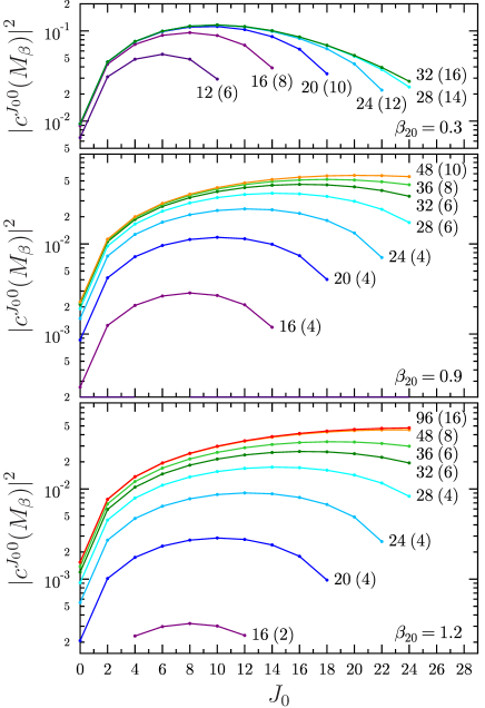
Figure 12: (Color online) Decomposition of the weights $\big{|}c^{J_{0}0}\big{|}^{2}$ of the projected components as defined in Eq. (121) on a logarithmic scale for axial reflection-symmetric states of ²⁴⁰Pu with dimensionless quadrupole moment $\beta_{20}$ and number of discretization points $M_{\beta}$ as indicated. The number in parentheses indicates the number of Euler angles whose contribution is at most ten orders of magnitude smaller than the largest one. Because of the reflection symmetry imposed on the quasiparticle vacua, the $\big{|}c^{J_{0}0}\big{|}^{2}$ are exactly zero for odd angular momenta and therefore not plotted.

Figure 12 shows the convergence of the numerical calculation of the weights $\big{|}c^{J_{0}0}\big{|}^{2}$ of the components at three different deformations as a function of $M_{\beta}$. The number of points in the full interval $0\leq\beta\leq\pi$ that is necessary to reach a sufficient level of convergence increases dramatically with deformation, which is again a direct consequence of the rule established in Eq. (117). It is, however, not necessary to evaluate the matrix elements at all of these integration points, as is indicated on Fig. 12 by the number of significant integration points given in the parentheses. In fact, to reach a similar level of convergence, the number of necessary significant integration points is similar in all three cases, but they do not cover the same range of Euler angles.

The Wigner $d$-matrix $d^{J_{0}}_{00}(\beta)$ equals the Legendre polynomial of order $J_{0}$ in $\cos(\beta)$ Varshalovich et al. (1988). As a consequence, when using the discretization (116) the weights $\big{|}c^{J_{0}0}\big{|}^{2}$ are numerically exactly zero for $J_{0}=M_{\beta}$, as in that case all abscissas coincide with the zeros of $d^{M_{\beta}}_{00}(\beta)$. Therefore, for discretizations with $M_{\beta}\leq 24$ the curves on Fig. 12 end at $J_{0}=M_{\beta}-2$. The weights of some components with $J_{0}\gg M_{\beta}$ are again numerically non-zero as in the examples discussed above, but have been omitted on Fig. 12 for the sake of clarity. From the discussion leading to Eq. (117) it is clear that the numerically calculated values of these components cannot be correct.

Assuming that $|\Phi_{a}\rangle$ is a normalized axial reflection-symmetric state, at small Euler angles $\beta$ the norm kernel for projection of that state can be estimated to be Baye and Heenen (1984)

$$\langle\Phi_{a}|\hat{R}(0,\beta,0)|\Phi_{a}\rangle\simeq\exp\big{\{}-[1-\cos(\beta)]\,\langle\Phi_{a}|\hat{J}^{2}_{\perp}|\Phi_{a}\rangle\big{\}}\,.$$ (124)

where $\hat{J}^{2}_{\perp}$ is the square of the expectation value of angular momentum in a direction perpendicular to the symmetry axis. As can be seen from Fig. 11, this estimate closely follows the calculated points for values of $\cos(\beta)$ between 1.0 and about 0.85, which is sufficient to estimate the range of Euler angles $\beta$ that will contribute significantly to the projected overlap and operator matrix elements. This information can be used to adapt $M_{\beta}$ such that one can expect to have a certain number of significant integration points, and also to optimize approximate schemes for angular momentum projection that rely on interpolation between a small number of exactly calculated kernels Bender et al. (2004b, 2006). If needed, higher-order corrections to Eq. (124) can also be derived. Generalizations of Eq. (124) to full 3d rotations of non-axial states as the ones given in Islam et al. (1979); Baye and Heenen (1984) can also be used to anticipate the number of discretization points needed to project more complex states.

To conclude, the number of discretization points for each Euler angle required to represent accurately the three-dimensional integral over Euler angles depends very sensitively on the nature and orientation of the state one starts with. The large variety of possible decompositions that can be encountered prevents the existence of a simple recipe for the selection of integration points that can be expected to be near-optimal for all situations. To achieve a numerically precise projection of irreps up to $J_{0}$ one needs an estimate of the largest values of $J$ and $K$ contained in decomposition of a given states, as well as an estimate of the width of the norm kernel as a function of the Euler angles. In certain cases, the number of significant discretization points that have to be evaluated numerically in order to reliably perform the angular-momentum projection can be as large as several times $10^{4}$.

V Projection of cranked triaxial quasiparticle states

V.1 General considerations

Even considering the simple structure of a Bogoliubov-type quasiparticle vacua, numerical calculations for completely symmetry-unrestricted Bogoliubov reference states are far from being trivial. Besides their numerical cost, there are also practical issues such as the necessity to fix the position of the center-of-mass and also the orientation of the nucleus when self-consistently constructing the reference states, which can become complicated to implement and delicate to converge. In addition, there is a large body of empirical evidence that for many phenomena of interest the self-consistent solution of the HFB equation adopts one or several symmetries, which can be used to simplify the numerical treatment by imposing these as intrinsic symmetries throughout the calculation.

All such conserved intrinsic space-time symmetries have in common that in one way or another they introduce linear dependences between the states in the vector space $\text{span}(SU(2)_{A}|\Phi\rangle)$ that can be constructed through rotations of a given Bogoliubov state $|\Phi\rangle$. This has two important consequences. First, these linear dependences can be used to reduce the number of rotated states that actually have to be constructed through application of the rotation operator. Second, these linear dependences reduce the number of different irreps $\epsilon$ for a given value of $J$ that a given Bogoliubov state $|\Phi\rangle$ can be decomposed into in Eq. (94), from $2J+1$ to a smaller number, sometimes even zero. The latter manifests itself either through vanishing matrix elements in the Hamiltonian and norm kernels of Eqns. (96) and (97), or through linear dependences between their respective matrix elements, which in either case reduces the rank of these matrices. We have seen already some examples for such reduction in Sect. IV.5. Ultimately, the linear dependences between rotated states can be exploited to reduce the number of actual matrix elements $\langle\Phi_{a}|\hat{T}^{\lambda}_{m}\hat{P}^{J}_{MK}|\Phi_{b}\rangle$ that have to be calculated numerically. Even more importantly, the reduction of the rank of the norm and Hamiltonian matrices might jeopardize the numerical solution of the the GEP (95) when not being taken care of.

As an example for the practical consequences of intrinsic symmetries, we will discuss here the case of time-reversal breaking triaxial HFB states, which offer the flexibility to cover a large number of cases of interest in nuclear spectroscopy Bender and Heenen (2008); Rodríguez and Egido (2010); Yao et al. (2011); Bally et al. (2014); Borrajo et al. (2015); Egido et al. (2016); Egido (2016), such as arbitrary quadrupole deformation and collective rotation about a principal axis. There are several possibilities how triaxial symmetry can be realized by imposing different subgroups of the double point symmetry group $D_{2h}^{TD}$ as defined in Dobaczewski et al. (2000a, b). To exemplify the procedure, we will use here the subgroup consisting of parity $\hat{P}$, the $x$-signature $\hat{R}_{x}$, and the $y$-time-simplex $\hat{S}^{\mathcal{T}}_{y}\equiv\hat{R}_{y}\hat{P}\hat{\mathcal{T}}$, with $\hat{\mathcal{T}}$ being the time-reversal operator. We will label the group generated by these three operators as $\langle\hat{P},\hat{R}_{x},\hat{S}^{\mathcal{T}}_{y}\rangle$.

This choice is not unique, and there are others that offer the same physical degrees of freedom Dobaczewski et al. (2000b), but differ by an exchange of coordinate axes. The actual specific choice of symmetry group has some consequences for the convenience of numerical implementations. The choice made here allows for simplifications during the mixing of $K$-components when solving the GEP that will be discussed in Sect. V.3. For single-reference calculations, however, it is of advantage to impose $z$-signature $\hat{R}_{z}$ instead of $x$-signature as described in Bonche et al. (1987). The transformation between both representations Bally (2014) can be achieved with an axis permutation operator as proposed in Ref. Bonche et al. (1991).

The symmetries of the quasiparticle vacua have actually to be implemented at the level of the one-quasiparticle states, meaning that one has to use a basis of single-particle states that respect this set of intrinsic symmetries, and construct Bogoliubov matrices that have the appropriate symmetry-preserving block structure. This has, however, no importance for our sidcussion. For further details we refer to Refs. Dobaczewski et al. (2000a, b).

Let us now specify the properties of a quasiparticle vacuum $|\Phi_{a}\rangle$ that has the symmetries of the group $\langle\hat{P},\hat{R}_{x},\hat{S}^{\mathcal{T}}_{y}\rangle$. This implies that

$$\hat{P}|\Phi_{a}\rangle =p_{a}\,|\Phi_{a}\rangle\,,$$ (125a)

$$\hat{R}_{x}|\Phi_{a}\rangle =\eta_{a}\,|\Phi_{a}\rangle\,,$$ (125b)

$$\hat{S}^{\mathcal{T}}_{y}|\Phi_{a}\rangle =\phantom{\pi_{a}}\,|\Phi_{a}\rangle\,,$$ (125c)

where only the first two relations are eigenvalue equations, whereas the third one for the anti-linear operator $\hat{S}^{\mathcal{T}}_{y}$ fixes a phase through a symmetry transformation Dobaczewski et al. (2000a, b). From $|\Phi_{a}\rangle$ being a fermionic product state one also automatically has the relations

$$\hat{\Pi}_{A}|\Phi_{a}\rangle =\pi_{a}\,|\Phi_{a}\rangle\,,$$ (126a)

$$\hat{R}_{\mu}^{2}|\Phi_{a}\rangle =\pi_{a}\,|\Phi_{a}\rangle\quad\text{for $\mu=x$, $y$, $z$,}$$ (126b)

$$\hat{\mathcal{T}}^{2}|\Phi_{a}\rangle =\pi_{a}\,|\Phi_{a}\rangle\,.$$ (126c)

for the number parity $\hat{\Pi}_{A}$ (59), squared signature $\hat{R}_{\mu}^{2}$ and the square of the time-reversal operator.

As we assume that $|\Phi_{a}\rangle$ is a direct product of a neutron and a proton many-body wave functions, and as our symmetry operators factorize in the corresponding tensor product space, for example $\hat{\Pi}_{A}\equiv\hat{\Pi}_{N}\otimes\hat{\Pi}_{Z}$, the total number parity $\pi_{a}$, total parity $p_{a}$, and total signature $\eta_{a}$, are then the products of the proton and neutron number parities, parities, and signatures, respectively,

$$\pi_{a} =\pi_{na}\,\pi_{za}\,$$ , (127a)

$$p_{a} =p_{na}\,p_{za}\,$$ , (127b)

$$\eta_{a} =\eta_{na}\,\eta_{za}\,$$ , (127c)

where if the particle species $q=n$, $p$, has even number parity we have

$$\pi_{qa}=+1\,,\quad p_{qa}=\pm 1\,,\quad\eta_{qa}=\pm 1\,,$$ (128)

whereas if the particle species $q$ has an odd number parity we have

$$\pi_{qa}=-1\,,\quad p_{qa}=\pm 1\,,\quad\eta_{qa}=\pm i\,.$$ (129)

Finally, defining a short-hand notation for the time-reversed state

$$|\overline{\Phi}_{a}\rangle=\hat{\mathcal{T}}\,|\Phi_{a}\rangle\,,$$ (130)

we can derive an additional useful relation between $|\Phi_{a}\rangle$ and its time-reversed $|\overline{\Phi}_{a}\rangle$ from (125)

$$\hat{R}_{z}|\Phi_{a}\rangle=\pi_{a}\,p_{a}\,\eta_{a}^{*}\,|\overline{\Phi}_{a}\rangle\,,$$ (131)

which follows from $\hat{S}^{T}_{y}\equiv\hat{R}_{y}\,\hat{P}\,\hat{\mathcal{T}}=\hat{R}_{z}\,\hat{R}_{x}\,\hat{P}\,\hat{\mathcal{T}}$. Further details about the derivation of these relations can be found in Ref. Bally (2014). As said above, quasiparticle vacua respecting these symmetries cover the vast majority of cases of interest for single-reference applications to nuclear spectroscopy. And we will see that these symmetries allow also for great simplifications at the multi-reference level.

We note that the symmetries of the $\langle\hat{P},\hat{R}_{x},\hat{S}^{\mathcal{T}}_{y}\rangle$ point-group can only be imposed on the unrotated states. The noncommutativity of rotations about different axes implies that the symmetry relations under $\hat{R}_{x}$ and $\hat{S}^{\mathcal{T}}_{y}$ transformations get lost when rotating a state to an arbitrary angle $\hat{R}(\alpha,\beta,\gamma)\,|\Phi_{a}\rangle$, such that only parity remains as a common symmetry of the rotated and unrotated states.

V.2 Symmetries of the rotated matrix elements

The numerical cost of the evaluation of an angular-momentum projected matrix element scales with the number $M_{\alpha}\times M_{\beta}\times M_{\gamma}$ of discretization points. As we have seen in Sect. IV.5, to numerically converge projected matrix elements might require to consider several tens of thousands of combinations of rotation angles, which can become a bottleneck in MR calculations that involve angular-momentum projection.

Therefore, to keep the computational time under control it is advantageous to find ways to reduce the number of angles that have to be calculated without altering the accuracy of the discretized integrals. By using the symmetries defined in Sect. V.1, we can derive a set of helpful relations between rotations by certain angles.

We will consider here the general case where we want to evaluate projected matrix elements of the $2\lambda+1$ components $m$ of a spherical tensor operator $\hat{T}^{\lambda}_{m}$ between two different reference states $|\Phi_{b}\rangle$ and $|\Phi_{a}\rangle$, which are assumed to have the same number parity for both protons and neutrons. Defining $\hat{\overline{T}}{}^{\lambda}_{m}\equiv\hat{\mathcal{T}}\,\hat{T}^{\lambda}_{m}\,\hat{\mathcal{T}}^{\dagger}$ as a shorthand for the operator obtained by a time-reversal transformation of $\hat{T}^{\lambda}_{m}$, we obtain the following seven relations Bally (2014)

$$\langle\Phi_{a}|\hat{R}(\pi-\alpha,\beta,\pi-\gamma)\,\hat{T}^{\lambda}_{m}|\Phi_{b}\rangle =(-)^{\lambda}\,\pi_{a}\,\eta_{a}\,\eta_{b}^{*}\, \langle\Phi_{a}|\hat{R}(\alpha,\beta,\gamma)\,\hat{T}^{\lambda}_{-m}|\Phi_{b}\rangle\,$$ , (132a)

$$\langle\Phi_{a}|\hat{R}(\pi+\alpha,\pi-\beta,2\pi-\gamma)\,\hat{T}^{\lambda}_{m}|\Phi_{b}\rangle =(-)^{\lambda}\,\pi_{a}\,\eta_{b}^{*}\, \langle\Phi_{a}|\hat{R}(\alpha,\beta,\gamma)\hat{T}^{\lambda}_{-m}|\Phi_{b}\rangle\,$$ , (132b)

$$\langle\Phi_{a}|\hat{R}(2\pi-\alpha,\pi-\beta,\pi+\gamma)\,\hat{T}^{\lambda}_{m}|\Phi_{b}\rangle =\pi_{a}\,\eta_{a}\, \langle\Phi_{a}|\hat{R}(\alpha,\beta,\gamma)\,\hat{T}^{\lambda}_{m}|\Phi_{b}\rangle\,$$ , (132c)

$$\langle\Phi_{a}|\hat{R}(\alpha,\pi-\beta,\pi-\gamma)\,\hat{T}^{\lambda}_{m}|\Phi_{b}\rangle =(-)^{\lambda+m}\,p_{a}\,p_{b}\,\eta_{a}\, \langle\Phi_{a}|\hat{R}(\alpha,\beta,\gamma)\,\hat{\overline{T}}{}^{\lambda}_{-m}|\Phi_{b}\rangle^{*}\,$$ , (132d)

$$\langle\Phi_{a}|\hat{R}(\pi-\alpha,\pi-\beta,\gamma)\,\hat{T}^{\lambda}_{m}|\Phi_{b}\rangle =(-)^{m}\,p_{a}\,p_{b}\,\eta_{b}^{*}\, \langle\Phi_{a}|\hat{R}(\alpha,\beta,\gamma)\,\hat{\overline{T}}{}^{\lambda}_{m}|\Phi_{b}\rangle^{*}\,$$ , (132e)

$$\langle\Phi_{a}|\hat{R}(\pi+\alpha,\beta,\pi+\gamma)\,\hat{T}^{\lambda}_{m}|\Phi_{b}\rangle =(-)^{m}\,\pi_{a}\,p_{a}\,p_{b}\,\eta_{a}\,\eta_{b}^{*}\, \langle\Phi_{a}|\hat{R}(\alpha,\beta,\gamma)\,\hat{\overline{T}}{}^{\lambda}_{m}|\Phi_{b}\rangle^{*}\,$$ , (132f)

$$\langle\Phi_{a}|\hat{R}(2\pi-\alpha,\beta,2\pi-\gamma)\,\hat{T}^{\lambda}_{m}|\Phi_{b}\rangle =(-)^{\lambda+m}\,p_{a}\,p_{b}\, \langle\Phi_{a}|\hat{R}(\alpha,\beta,\gamma)\,\hat{\overline{T}}{}^{\lambda}_{-m}|\Phi_{b}\rangle^{*}\,$$ , (132g)

Each of these relations is obtained by replacing either the left and/or right quasiparticle vacuum entering the matrix element with a suitable symmetry-transformed state from one of the relations in Eq. (125) or (126), followed by commutation of the rotation operator contained in the symmetry transformation with $$\hat{T}^{\lambda}_{m} \pi (\alpha,\beta,\gamma)$$ according to Eq. (107), using the special values of the Wigner rotation matrices at rotation angles that are multiples of Varshalovich et al. (1988) and regrouping of the remaining rotation operators into a single one Bally (2014). The above relations connect the matrix elements of any irreducible tensor operator at Euler angles with those at seven other combinations of Euler angles in the full integration interval of the discretized projection operator (118), which reduces the necessary computational cost of the projected matrix element by a factor of eight.

In addition to these relations, there is another one that relates matrix elements involving the time-reversed of one of the states with matrix elements at a different rotation angle

$$\langle\Phi_{a}| \hat{R}(\alpha,\beta,\pi+\gamma)\,\hat{T}^{\lambda}_{m}|\Phi_{b}\rangle$$

$$=(-)^{m}\,p_{b}\,\eta_{b}^{*}\,\langle\overline{\Phi}_{a}|\hat{R}(\alpha,\beta,\gamma)\,\hat{\overline{T}}{}^{\lambda}_{m}|\Phi_{b}\rangle^{*}\,.$$ (132h)

This relation is different in several respects from those of Eqns. (132a-132g). First, it only is a symmetry relation when time-reversal is conserved, i.e. when $|\overline{\Phi}_{a}\rangle=|\Phi_{a}\rangle$. In the more general case that we address here the matrix element on the r.h.s. of Eq. (V.2) still has to be numerically evaluated in addition to the one on the r.h.s. of Eqns. (132a-132g). However, constructing the time-reversed of a product state is usually much less costly, and numerically more precise, than rotating it. Second, relation (V.2) can be combined with any of the seven relations (132a-132g) above, such that the number of necessary applications of the rotation operator is reduced by a factor of 16, from the full interval $[0,2\pi]\times[0,\pi]\times[0,2\pi]$ to the much smaller one $\left[0,\frac{\pi}{2}\right]\times\left[0,\frac{\pi}{2}\right]\times\left[0,\pi\right]$. But for each of the remaining combinations of angles ($\alpha,\beta,\gamma$), one has to construct two matrix elements, one involving the original state, the other its time-reversed. Omitting global pre-factors, the application of the reduced angular momentum projection operator (106) becomes with this

$$\int^{2\pi}_{0}d\alpha\,\int^{\pi}_{0}d\beta\,\sin(\beta)\,\int^{2\pi}_{0}d\gamma\,D_{MK}^{J*}(\alpha,\beta,\gamma)\,\langle\Phi_{a}|\hat{R}(\alpha,\beta,\gamma)\hat{T}^{\lambda}_{m}|\Phi_{b}\rangle$$

$$=\int^{\frac{\pi}{2}}_{0}d\alpha\,\int^{\frac{\pi}{2}}_{0}d\beta\,\sin(\beta)\,\int^{\pi}_{0}d\gamma\,\Bigg{[}\bigg{\{}\Big{[}D_{MK}^{J*}(\alpha,\beta,\gamma)\,+\pi_{a}\eta_{a}D_{MK}^{J*}(2\pi-\alpha,\pi-\beta,\pi+\gamma)\Big{]}\langle\Phi_{a}|\hat{R}(\alpha,\beta,\gamma)\hat{T}^{\lambda}_{m}|\Phi_{b}\rangle$$

$$+(-)^{\lambda}\Big{[}\pi_{a}\eta_{a}\eta_{b}^{*}D_{MK}^{J*}(\pi-\alpha,\beta,\pi-\gamma)+\pi_{a}\eta_{b}^{*}D_{MK}^{J*}(\pi+\alpha,\pi-\beta,2\pi-\gamma)\,\Big{]}\langle\Phi_{a}|\hat{R}(\alpha,\beta,\gamma)\hat{T}^{\lambda}_{-m}|\Phi_{b}\rangle$$

$$+(-)^{m}\Big{[}p_{a}p_{b}\eta_{b}^{*}D_{MK}^{J*}(\pi-\alpha,\pi-\beta,\gamma)+\pi_{a}p_{a}p_{b}\eta_{a}\eta_{b}^{*}D_{MK}^{J*}(\pi+\alpha,\beta,\pi+\gamma)\Big{]}\langle\Phi_{a}|\hat{R}(\alpha,\beta,\gamma)\hat{\overline{T}}{}^{\lambda}_{m}|\Phi_{b}\rangle^{*}$$

$$+(-)^{\lambda+m}\Big{[}p_{a}p_{b}\eta_{a}D_{MK}^{J*}(\alpha,\pi-\beta,\pi-\gamma)+p_{a}p_{b}D_{MK}^{J*}(2\pi-\alpha,\beta,2\pi-\gamma)\Big{]}\langle\Phi_{a}|\hat{R}(\alpha,\beta,\gamma)\hat{\overline{T}}{}^{\lambda}_{-m}|\Phi_{b}\rangle^{*}\bigg{\}}$$

$$+(-)^{m}p_{b}\eta_{b}^{*}\bigg{\{}\Big{[}D_{MK}^{J*}(\alpha,\beta,\pi+\gamma)\,+\pi_{a}\eta_{a}D_{MK}^{J*}(2\pi-\alpha,\pi-\beta,2\pi+\gamma)\Big{]}\langle\overline{\Phi}_{a}|\hat{R}(\alpha,\beta,\gamma)\hat{\overline{T}}{}^{\lambda}_{m}|\Phi_{b}\rangle^{*}$$

$$+(-)^{\lambda}\Big{[}\pi_{a}\eta_{a}\eta_{b}^{*}D_{MK}^{J*}(\pi-\alpha,\beta,-\gamma)+\pi_{a}\eta_{b}^{*}D_{MK}^{J*}(\pi+\alpha,\pi-\beta,\pi-\gamma)\,\Big{]}\langle\overline{\Phi}_{a}|\hat{R}(\alpha,\beta,\gamma)\hat{\overline{T}}{}^{\lambda}_{-m}|\Phi_{b}\rangle^{*}\bigg{\}}$$

$$+(-)^{m}p_{b}\eta_{b}\bigg{\{}(-)^{m}\Big{[}p_{a}p_{b}\eta_{b}^{*}D_{MK}^{J*}(\pi-\alpha,\pi-\beta,\pi+\gamma)+\pi_{a}p_{a}p_{b}\eta_{a}\eta_{b}^{*}D_{MK}^{J*}(\pi+\alpha,\beta,2\pi+\gamma)\Big{]}\langle\overline{\Phi}_{a}|\hat{R}(\alpha,\beta,\gamma)\hat{T}^{\lambda}_{m}|\Phi_{b}\rangle$$

$$+(-)^{\lambda+m}\Big{[}p_{a}p_{b}\eta_{a}D_{MK}^{J*}(\alpha,\pi-\beta,-\gamma)+p_{a}p_{b}D_{MK}^{J*}(2\pi-\alpha,\beta,\pi-\gamma)\Big{]}\langle\overline{\Phi}_{a}|\hat{R}(\alpha,\beta,\gamma)\hat{T}^{\lambda}_{-m}|\Phi_{b}\rangle\bigg{\}}\Bigg{]}\,.$$ (133)

The above equation is valid whatever the eigenvalue of the $x$-signature and whatever the number parity of the considered quasiparticle vacua. Thereby, this equation constitutes a generalization of the expression given in Ref. Enami et al. (1999) that is limited to quasiparticle vacua with a $x$-signature $\eta_{a}=\eta_{na}=\eta_{pa}=1$ describing even-even nuclei.

As already mentioned when defining them through Eqns. (114) and (116), respectively, the use of the symmetries (132a-V.2) of the rotated matrix elements imposes some conditions on the form of the discretized operators $\hat{\mathbb{P}}^{K_{0}}_{z,M_{\gamma}}$ and $\hat{\mathbb{P}}^{J_{0}M_{0}K_{0}}_{y,M_{\beta}}$. First, the angles connected by the symmetries have all to be contained in a given discretization of the complete intervals. Second, it should be avoided that discretization points are located on the borders of the reduced intervals $\left[0,\frac{\pi}{2}\right]\times\left[0,\frac{\pi}{2}\right]\times\left[0,\pi\right]$. Indeed, when the quasiparticle vacua have eigenvalues of parity or signature that are different from $+1$, or when the two states entering the matrix element have different signature, then (132a-V.2) imply that for symmetry reasons the norm overlap and some other operator matrix elements are zero on some of the boundaries of the reduced integration intervals. Using a discretization with points on the boundaries would then implicitly reduce the order of the quadrature rules. In addition, the same technical problems already mentioned in Sect. III.6 would present themselves for the evaluation of those operator kernels that remain non-zero at those angles.

The definitions Eqns. (114) and (116) of the discretized projection operators respect these requirements as long as the values of $M_{\alpha}$, $M_{\beta}$, and $M_{\gamma}$ are chosen to be of the form

$$\begin{split}M_{\alpha}&=4i\,,\\ M_{\beta}&=2j\qquad i,j,k\in\mathbb{N}\,,\\ M_{\gamma}&=2k\,,\end{split}$$ (134)

because we reduced by a factor of four, two, and again two the three intervals on which we carry out the rotations over $\alpha$, $\beta$, and $\gamma$, respectively.

V.3 Mixing of $K$-components

As discussed in Sec. II on the general principles of symmetry projection, linear dependences among the rotated states as discussed in the previous subsection result in a reduction of the dimensionality of the subspace they span. While for some intrinsic symmetries this eliminates specific values of $J$ and/or $K$ directly from the spectrum of components a given quasiparticle vacuum can be decomposed into, working with eigenstates of the $x$-signature introduces a symmetry in the norm and operator kernels that has to be specifically taken care of.

Indeed, considering a quasiparticle state $|\Phi_{a}\rangle$ that is an irrep of $\langle\hat{P},\hat{R}_{x},\hat{S}^{\mathcal{T}}_{y}\rangle$, a rotation by an angle $\pi$ around the $x$-axis transforms its projected component $K$ into its projected component $-K$

$$\hat{R}_{x}|\Psi^{JK}_{a\epsilon}\rangle=e^{-\text{i}\pi J}\,|\Psi^{J-K}_{a\epsilon}\rangle\,,$$ (135)

which can be easily shown inserting Eq. (85a) into Eq. (89) and then using the special values of the Wigner function $D_{MK}^{J}(0,\pi,\pi)$ Varshalovich et al. (1988) for given $J$, $M$, and $K$. This relation implies that the coefficients $c^{J\pm K}_{a\epsilon}$ in the decomposition (99) are related through

$$c^{J-K}_{a\epsilon}=\eta_{a}\,e^{+\text{i}\pi J}\,c^{JK}_{a\epsilon}\,.$$ (136)

This relation among the weights of the components that can be projected out from a state with given signature translates into a symmetry relation among elements (97) of the projected norm matrix $\boldsymbol{N}^{J}$

$$N_{KK^{\prime}}^{J} =\eta_{a}\,e^{+\text{i}\pi J}\, N_{K-K^{\prime}}^{J}\,,$$ (137a)

$$=\eta_{a}^{*}\,e^{-\text{i}\pi J}\, N_{-KK^{\prime}}^{J}\,,$$ (137b)

$$= N_{-K-K^{\prime}}^{J}\,,$$ (137c)

These relations imply that the norm matrix has null eigenvalues whenever decomposing a state with good $x$-signature. More precisely, there are $d_{\text{null}}=\frac{2J+1}{2}$ of them for half-integer angular momenta, and $d_{\text{null}}=\frac{2J+1}{2}\pm\frac{1}{2}$ of them for integer angular momenta (the sign for $\pm 1/2$ depends on whether ${N}^{J}_{00}$ is null for reason of other intrinsic symmetries or not). Notice that this does not necessarily exhaust the number of zero norm eigenvalues of these matrices as others can be null as well , for example, for reason of additional intrinsic symmetries that are not imposed by the numerical representation, but that are self-consistently taken by the state.

As the Hamiltonian is rotationally invariant, it commutes with $\hat{R}_{x}$ and we find analogous symmetry relations for the elements (96) of the Hamiltonian matrix $\boldsymbol{H}^{J}$

$$H_{KK^{\prime}}^{J} =\eta_{a}\,e^{+\text{i}\pi J}\, H_{K-K^{\prime}}^{J}\,,$$ (138a)

$$=\eta_{a}^{*}\,e^{-\text{i}\pi J}\, H_{-KK^{\prime}}^{J}\,,$$ (138b)

$$= H_{-K-K^{\prime}}^{J}\,.$$ (138c)

To solve the GEP (95) numerically, we have to first remove all the null eigenvalues of the norm matrix that arise because of the intrinsic $x$-signature symmetry. In order to do so, we extend on an idea proposed by Enami et al. Enami et al. (1999), that is, we realize a similarity transformation that partitions the norm, Hamiltonian, and other operator matrices into a $d_{\text{null}}\times d_{\text{null}}$ block that acts in the null space arising from the intrinsic $x$-signature symmetry, and a $(2J+1-d_{\text{null}})\times(2J+1-d_{\text{null}})$ block in the remaining space of vectors that are not connected by a signature transformation. For the simplest case of states $|\Phi_{a}\rangle$ with even number parity of protons and neutrons and positive $x$-signature $\eta_{a}=+1$, a possible choice for $\boldsymbol{W}$ has been given in Ref. Enami et al. (1999). The generalization to arbitrary number parities and eigenvalues of signature is straightforward.

For a Bogoliubov quasiparticle vacuum $|\Phi_{a}\rangle$ with even number parity and $x$-signature $\eta_{a}=\pm 1$, which implies projection onto integer angular momentum $J$, the transformation $\boldsymbol{W}$ can be taken as the $(2J+1)\times(2J+1)$ orthogonal matrix

$$\boldsymbol{W}^{J}_{\eta_{a}}\equiv\left(\begin{array}[]{ccccccc}\tfrac{1}{\sqrt{2}}&&&\mbox{\large 0}&&&\tfrac{\eta_{a}(-)^{J}}{\sqrt{2}}\phantom{a}\\ &\ddots&&&&\iddots&\\ &&\tfrac{1}{\sqrt{2}}&&\tfrac{\eta_{a}(-)^{J}}{\sqrt{2}}\phantom{a}&&\\ \mbox{\large 0}&&&1&&&\mbox{\large 0}\\ &&\tfrac{\eta_{a}(-)^{J+1}}{\sqrt{2}}&&\tfrac{1}{\sqrt{2}}&&\\ &\iddots&&&&\ddots&\\ \tfrac{\eta_{a}(-)^{J+1}}{\sqrt{2}}&&&\mbox{\large 0}&&&\tfrac{1}{\sqrt{2}}\end{array}\right)\,.$$ (139)

Using relations (137) along the way, the norm matrix resulting from a similarity transformation with this matrix takes the structure

$$\big{(}{\boldsymbol{W}^{J}_{\eta_{a}}}\big{)}^{-1} \boldsymbol{N}^{J}\,\boldsymbol{W}_{\eta_{a}}^{J}$$

$$= \left(\begin{array}[]{@{}c|c|c@{}}\phantom{\mbox{\large 0}}&&\phantom{\mbox{\large 0}}\\ \mbox{\large 0}&\mbox{\large 0}&\mbox{\large 0}\\ \phantom{\mbox{\large 0}}&&\phantom{\mbox{\large 0}}\\ \hline\cr\phantom{\Big{|}}\mbox{\large 0}\phantom{\Big{|}}&N^{J}_{00}&\sqrt{2}N^{J}_{01}\cdots\sqrt{2}N^{J}_{0J}\\ \hline\cr\phantom{yolo}\mbox{\large 0}\phantom{yolo}&\begin{matrix}\sqrt{2}N^{J}_{10}\\ \vdots\\ \sqrt{2}N^{J}_{J0}\end{matrix}&\begin{matrix}2N^{J}_{11}&\cdots&2N^{J}_{1J}\\ \vdots&\ddots&\vdots\\ 2N^{J}_{J1}&\cdots&2N^{J}_{JJ}\\ \end{matrix}\end{array}\right)$$ (145)

$$\equiv \left(\begin{matrix}\mbox{0}&\mbox{0}\\ \mbox{0}&\tilde{\boldsymbol{N}}^{J}\end{matrix}\right)\,,$$ (146)

and similar for the transformed Hamiltonian matrix and the matrices representing other operators.

For a Bogoliubov quasiparticle vacuum $|\Phi_{a}\rangle$ with odd number parity and $x$-signature $\eta_{a}=\pm i$, which implies projection onto half-integer angular momentum $J$, $\boldsymbol{W}^{J}_{\eta_{a}}$ can be taken as the $(2J+1)\times(2J+1)$ orthogonal matrix

$$\boldsymbol{W}^{J}_{\eta_{a}}\equiv\left(\begin{array}[]{ccccccc}\tfrac{1}{\sqrt{2}}&&&\mbox{\large 0}&&&\tfrac{\eta_{a}e^{+\text{i}\pi J}}{\sqrt{2}}\\ &\ddots&&&&\iddots&\\ &&\tfrac{1}{\sqrt{2}}&&\tfrac{\eta_{a}e^{+\text{i}\pi J}}{\sqrt{2}}&&\\ \mbox{\large 0}&&&&&&\mbox{\large 0}\\ &&\tfrac{\eta_{a}e^{-\text{i}\pi J}}{\sqrt{2}}&&\tfrac{1}{\sqrt{2}}&&\\ &\iddots&&&&\ddots&\\ \tfrac{\eta_{a}e^{-\text{i}\pi J}}{\sqrt{2}}&&&\mbox{\large 0}&&&\tfrac{1}{\sqrt{2}}\\ \end{array}\right)\,.$$ (147)

In that case, the similarity-transformed norm matrix takes the form

$$\big{(}{\boldsymbol{W}^{J}_{\eta_{a}}}\big{)}^{-1}\,\boldsymbol{N}^{J}\,\boldsymbol{W}_{\eta_{a}}^{J}= \left(\begin{array}[]{@{}c|c@{}}\phantom{\mbox{\large 0}}&\phantom{\mbox{\large 0}}\\ \mbox{\large 0}&\mbox{\large 0}\\ \phantom{\mbox{\large 0}}&\phantom{\mbox{\large 0}}\\ \hline\cr\phantom{yolo}\mbox{\large 0}\phantom{yolo}&\begin{matrix}2N^{J}_{\frac{1}{2}\frac{1}{2}}&\cdots&2N^{J}_{\frac{1}{2}J}\\ \vdots&\ddots&\vdots\\ 2N^{J}_{J\frac{1}{2}}&\cdots&2N^{J}_{JJ}\\ \end{matrix}\end{array}\right)$$ (152)

$$\equiv \left(\begin{matrix}\mbox{0}&\mbox{0}\\ \mbox{0}&\tilde{\boldsymbol{N}}^{J}\end{matrix}\right)\,.$$ (153)

We remark that, in the general case, the transformation matrix $\boldsymbol{W}^{J}_{\eta_{a}}$ does not only depend on the angular momentum onto which one projects, but also on the $x$-signature $\eta_{a}$ of the state $|\Phi_{a}\rangle$.

The advantage of performing such transformation is that it replaces the GEP (95) that has $d_{\text{null}}$ zero eigenvalues for symmetry reasons by a GEP that is reduced to the $(2J+1-d_{\text{null}})\times(2J+1-d_{\text{null}})$ non-trivial blocks $\boldsymbol{\tilde{N}}^{J}$ and $\boldsymbol{\tilde{H}}^{J}$ of the transformed norm and Hamiltonian matrices

$$\boldsymbol{\tilde{H}}^{J}\boldsymbol{\tilde{f}}^{J}_{\epsilon}=e^{J}_{\epsilon}\boldsymbol{\tilde{N}}^{J}\boldsymbol{\tilde{f}}^{J}_{\epsilon}\,.$$ (154)

The transformed generalized eigenvectors $\boldsymbol{\tilde{f}}^{J}_{\epsilon}$ are related to the original ones through

$$\left(\begin{matrix}\boldsymbol{0}\\ \boldsymbol{\tilde{f}}^{J}_{\epsilon}\end{matrix}\right)=\boldsymbol{W}^{-1}_{\eta_{a}}\,\boldsymbol{f}^{J}_{\epsilon}$$ (155)

and are a linear combination of projected components with $K$ and $-K$ components induced by the $x$-signature symmetry. The possibility to eliminate the redundant components this way is what has motivated us to choose the $x$-signature in the angular momentum projection over the $z$-signature used in single-reference calculations.

The new GEP of Eq. (154) obtained after similarity transformation gives same generalized eigenvalues $e^{J}_{\epsilon}$ as the ones of the original GEP. As for projected states, they can be shown to be equivalent to the original ones. Therefore we obtain same results by solving the transformed problem.

The definition of the transformation $\boldsymbol{W}^{J}_{\eta_{a}}$ is not unique; there are possible alternative forms that differ by global phases or that result in a different placement of the non-trivial block in the transformed matrix. But all of these lead to the same projected states after solution of the GEP.

The above relations can be easily generalized to the transformation of the norm and energy kernels between two different states as they enter the a GCM calculation based on angular-momentum projected states, and which are simply obtained as $\big{(}{\boldsymbol{W}^{J}_{\eta_{a}}}\big{)}^{-1}\,\boldsymbol{N}^{aJbJ}\,\boldsymbol{W}_{\eta_{b}}^{J}$ and similar for the energy kernel. The same relation can also be used to transform the matrices representing the matrix elements of any other scalar operator to the reduced space.

For higher-rank tensor operators that connect different irreps, the transformation of the initial and final state will in general be different as their angular momenta and signatures can be different. For a set of tensor operators $\hat{T}^{\lambda}_{\mu}$, and defining the reduced matrix elements before $K$-mixing as

$$\boldsymbol{T}^{aJ^{\prime}bJ}_{K^{\prime}K}\,\equiv\, \sqrt{2J^{\prime}+1}\sum_{\mu=-\lambda}^{\lambda}\sum_{M=-J}^{J}\left(JM\lambda\mu|J^{\prime}K^{\prime}\right)$$

$$\times\langle\Phi_{a}|\hat{T}^{\lambda}_{\mu}\hat{P}^{J}_{MK}|\Phi_{b}\rangle\,,$$ (156)

one then has to compute in the general case the transformed matrix

$$\left(\begin{array}[]{@{}c|c@{}}\phantom{\boldsymbol{\tilde{T}^{aJ}}}&\phantom{\mbox{0}}\\ \hline\cr\phantom{\mbox{0}}&\boldsymbol{\tilde{T}}^{aJ^{\prime}bJ}\end{array}\right)\equiv\big{(}{\boldsymbol{W}^{J^{\prime}}_{\eta_{a}}}\big{)}^{-1}\,\boldsymbol{T}^{aJ^{\prime}bJ}\,\boldsymbol{W}_{\eta_{b}}^{J}\,,$$ (159)

where $\boldsymbol{\tilde{T}}^{aJ^{\prime}bJ}$ is now a $(2J^{\prime}+1-d^{\prime}_{\text{null}})\times(2J+1-d_{\text{null}})$ rectangular matrix.

V.4 Time-reversed partners

Let us consider a state $|\Phi_{a}\rangle$ and its time-reversed partner $|\overline{\Phi}_{a}\rangle$ as defined in Eq. (130). Using the symmetry relation (131), one can derive Bally (2014) that their components $c^{JK}_{a\epsilon}$ and $\bar{c}^{JK}_{a\epsilon}$, respectively, in the decomposition on the basis states of $\text{span}(SU(2)|\Phi_{a}\rangle)$ are related through the equation

$$\bar{c}^{JK}_{a\epsilon}=p_{a}\,\eta_{a}\,e^{+\text{i}\pi K}\,c^{JK}_{a\epsilon}\,.$$ (160)

As a consequence, the elements of the norm matrix $\boldsymbol{\bar{N}}^{J}$ for the time-reversed state $|\overline{\Phi}_{a}\rangle$ are directly related to those of $\boldsymbol{N}^{J}$ through the relation

$$\bar{N}^{J}_{KK^{\prime}}=(-)^{K-K^{\prime}}\,N^{J}_{KK^{\prime}}\,.$$ (161)

As the Hamiltonian commutes with $\hat{\mathcal{T}}$, we also have an equivalent relation for the Hamiltonian matrix $\boldsymbol{\bar{H}}^{J}$ of the time-reversed state $|\overline{\Phi}_{a}\rangle$

$$\bar{H}^{J}_{KK^{\prime}}=(-)^{K-K^{\prime}}\,H^{J}_{KK^{\prime}}\,.$$ (162)

Equations (161) and (162) can be seen as a similarity transformation through the $(2J+1)\times(2J+1)$ diagonal unitary matrix $\boldsymbol{S}$ whose matrix elements are

$$S_{KK^{\prime}}=e^{-\text{i}\pi K}\,\delta_{KK^{\prime}}\,.$$ (163)

With the same rationale as the one used in the previous section, it is then straightforward to understand that a pair of time-reversed states gives the same projected states after $K$-mixing, up to a phase factor. As example, we mention the case of two one-quasiparticle states built by blocking in a Bogoliubov even-even vacuum the two time-reversed single-particle states of opposite signatures. Even if they are orthogonal, those two one-quasiparticle states will give, up to linear dependence, the same projected states. As a result, when building projected states, it is sufficient to consider only one out of the two states $|\Phi_{a}\rangle$ and $|\overline{\Phi}_{a}\rangle$, but not both of them.

V.5 Reduction to a real symmetric GEP

Another relation can be obtained by noticing that, within basis states of an irrep of $SU(2)$, the time-reversal operation links a state with $K$ and a state with $-K$. With our choice of representation for the rotation and time-reversal operators, we obtain

$$\bar{c}^{JK}_{a\epsilon}=(-)^{J+K}\,\big{(}{c}^{J-K}_{a\epsilon}\big{)}^{*}\,.$$ (164)

Combining this relation with Eqs. (136) and (160), we identify that

$${c}^{JK}_{a\epsilon}=p_{a}\,(-)^{2J}\,\big{(}{c}^{JK}_{a\epsilon}\big{)}^{*}\,.$$ (165)

As a result, depending on the parity of the state $|\Phi_{a}\rangle$ and on the value of $J$, the weights ${c}^{JK}_{a\epsilon}$ are either real or purely imaginary numbers. Therefore, any product of the form $\big{(}{c}^{JK^{\prime}}_{a\epsilon}\big{)}^{*}{c}^{JK}_{a\epsilon}$ is real, and consequently so are the norm matrix $\boldsymbol{N}^{J}$ and the Hamiltonian matrix $\boldsymbol{H}^{J}$. The final consequence is that our problem reduces to a real symmetric GEP.

V.6 Representative applications

V.6.1 Examples of decomposition

label	$\langle\hat{Z}\rangle$	$\langle\hat{N}\rangle$	$(\beta_{2},\gamma)$	$\eta$	$p$	$\langle\hat{d}_{z}\rangle$	$\langle\hat{d}_{z}\rangle_{\text{axial}}$
“spherical”	12	13	$(0.0,0^{\circ})$	$-i$	1	0.50	0.50
“axial”	12	13	$(0.52,0^{\circ})$	$-i$	1	0.50	0.50
“triaxial 1”	12	13	$(0.60,14^{\circ})$	$-i$	1	0.65	0.50
“triaxial 2”	12	13	$(0.77,30^{\circ})$	$-i$	1	1.19	2.50

Table 3: Characteristics of the quasiparticle vacua discussed in Fig. 13, where $\beta_{2}$ and $\gamma$ are defined as in Ref. Bender and Heenen (2008) characterize the absolute size and non-axiality of quadrupole deformation, while $\eta$ is the eigenvalue of $z$-signature $\hat{R}_{z}$, $p$ the eigenvalue of parity, and $\langle\hat{d}_{z}\rangle$ the $z$ component of the decoupling vector as defined in Olbratowski et al. (2006) that for states with $\langle\hat{P},\hat{R}_{x},\hat{S}^{\mathcal{T}}_{y}\rangle$ plays the role of measuring the $z$ component of total angular momentum in the non-projected state (see text). We also give the value of the decoupling vector $\langle\hat{d}_{z}\rangle_{\text{axial}}$ of the equivalent single-particle state when considering a pure axial deformation. All states are constructed as blocked one-quasiparticle excitations of ²⁵Mg and therefore are odd under time-reversal.

Let us first study the decompositions in terms of $J$- and $K$-components of some quasiparticle vacua that have the intrinsic symmetries of the group $\langle\hat{P},\hat{R}_{x},\hat{S}^{\mathcal{T}}_{y}\rangle$. For a product state having such point-group symmetry all local densities and currents have three plane symmetries Dobaczewski et al. (2000a, b); Bonche et al. (1987). Examples of the decomposition of time-reversal-invariant quasiparticle vacua with even number parities for protons and neutrons that have this symmetry, which implies $p=\eta=+1$, have been discussed earlier in Refs. Bender and Heenen (2008); Rodríguez and Egido (2010). We consider here instead four different one-quasiparticle states of ²⁵Mg constructed by (self-consistently) blocking different selected single-particle states and imposing constraints on their average quadrupole deformation during the minimization procedure. These states are taken from the set of reference states entering the projected GCM calculation presented in Ref. Bally et al. (2014) and have been selected because they are representative examples for the effects of projection. The states were generated using the cartesian 3d coordinate-space HFB code CR8 that is based on the principles outlined in Ref. Bonche et al. (1987) and which has been updated to handle the Skyrme Hamiltonian SLyMR0 of Ref. Sadoudi et al. (2013) in connection with exact Coulomb exchange and Coulomb pairing, and which was used for the calculation described below. The HFB and the projection code Bender et al. use the same accurate Lagrange-mesh technique for derivatives Ryssens et al. (2015), which can also be used to define rotation operators. While the projection code assumes a $\langle\hat{P},\hat{R}_{x},\hat{S}^{\mathcal{T}}_{y}\rangle$ point-group symmetry, the mean-field code imposes a $\langle\hat{P},\hat{R}_{z},\hat{S}^{\mathcal{T}}_{y}\rangle$ symmetry instead, which is of advantage when generating cranked HFB states as those that will be discussed in Sect. V.6.3. The transformation between both representations is achieved with an axis permutation operator as defined in Ref. Bonche et al. (1991), see Ref. Bally (2014) for details. The main characteristics of the states can be found in Tab. 3. For the sake of simplicity we label the four states as “spherical”, “axial” and “triaxial”, which refers to the shape of their matter density distribution. In all cases, the shape has been constrained with quadrupole constraints that lead to the values for the quadrupole moments $\beta_{2}$ and $\gamma$. This does, however not mean that the “spherical” state truly takes spherical symmetry. While it has zero quadrupole moments, the distributions of spin and current cannot be spherically symmetric for a state with odd-number parity that in general has a non-zero expectation value of angular momentum. Similarly, the “axial” state has been constrained to an axial shape of its matter density distribution, which does not automatically mean that currents and spin densities are axially symmetric.

Working with eigenstates of the $x$-signature implies that only the component of their angular momentum vector pointing in $x$ direction is measurable; hence, can have a non-zero expectation value. This has direct consequences for the decomposition of such states into eigenstates of $\hat{J}_{z}$ by applying the projection operator $\hat{P}^{J}_{KK}$. As has been worked out in detail in Ref. Olbratowski et al. (2006), eigenstates of a signature with respect to some cartesian coordinate axis can always be expressed as a superposition of an eigenstate of a signature with respect to a different cartesian coordinate axis and its time-reversed state, where both have equal weight and some relative phase. As they are eigenstates of $\hat{J}_{z}$, the $K$ components projected out with $\hat{P}^{J}_{KK}$ are by construction also eigenstates of the $z$-signature. From this follows that a quasiparticle vacuum that is eigenstate of the $x$-signature will always decompose into pairs of components $\pm K$ with equal weight, which is the foundation of Eq. (136) derived earlier. The transformation $\boldsymbol{W}^{J}_{\eta}$ as defined in Eqns. (139) or (147) then recombines each pair of components $\pm K$ into a single state whose measurable angular momentum points again into $x$ direction. This choice of the $x$-axis for the direction of measurable angular momenta might not be the most intuitive, but has the advantage that redundant states in the decomposition can be eliminated with symmetry arguments based on conserved signature of the reference state. We also recall that the physical states are those obtained from $K$ mixing solving the GEP (154), such that the decomposition into $K$ components is merely a diagnostic tool. The following analysis of decomposition addresses $J$ and $K$ components as obtained from the application of $\hat{P}^{J}_{KK}$ before applying the similarity transformation $\boldsymbol{W}^{J}_{\eta}$.

The same arguments apply to the characterization of angular momenta of the quasiparticle vacua that serve as reference states. The shape of the states is oriented such that prolate states ($\gamma=0^{\circ}$) are symmetric around the $z$-axis in the projection code. The size of the angular momentum of a single-particle state along the symmetry axis of the “axial” state is obtained as the length of the “decoupling vector”’ $d_{z}\equiv\langle\hat{j}_{z}\,\hat{\mathcal{T}}\rangle$ as defined in Ref. Olbratowski et al. (2006). The same orientation has been chosen also for the “spherical” state.

In Fig. 13, we plot the two sums of components

$$\Xi^{J} \equiv\sum_{K=-J}^{J}\langle\Phi|\hat{{P}}^{J}_{KK}\hat{P}^{Z}\hat{P}^{N}|\Phi\rangle\,,$$ (166)

$$\Xi_{K} \equiv\sum_{J}\langle\Phi|\hat{{P}}^{J}_{KK}\hat{P}^{Z}\hat{P}^{N}|\Phi\rangle\,,$$ (167)

for the four quasiparticle vacua as specified in Tab. 3. In addition to angular-momentum restoration, all states were also projected on proton number $Z=12$ and neutron number $N=13$.

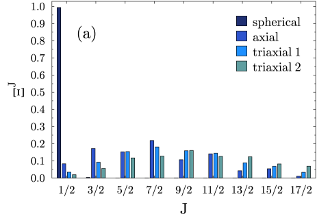
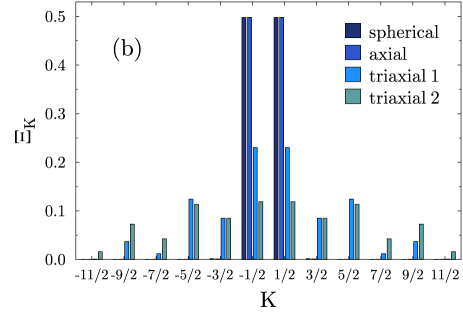
Figure 13: (Color online) Top: quantity $\Xi^{J}$ for the selected quasiparticles states discussed in the text. Bottom: same for the quantity $\Xi_{J}$.

As can been observed, the decompositions of the four states are very different one from another, but they all respect the symmetry $\Xi_{K}=\Xi_{-K}$, which is a consequence of the conserved $x$-signature of the reference state. This is to be contrasted with the more general asymmetric decomposition of state (b) discussed in Sec. IV.5 whose expectation value of angular momentum is not constrained by symmetry to point into a specific direction.

For the “spherical” state, we can see that it has an almost pure $J=1/2$ and $|K|=1/2$ character, the values being a fingerprint of the blocked $2s_{1/2}$ single-particle state in the canonical basis of the quasiparticle vacuum Ring and Schuck (1980). Because of the constraint on vanishing quadrupole moments, polarization effects are tiny as components with different $J$ and $K$ are barely visible on the scale of Fig. 13. It is also remarkable that, although the numerical representation on a three-dimensional cartesian mesh is not closed under rotations, an almost pure eigenstate of angular momentum $J$ state can be created simply through a constraint on its average deformation.

The state labeled “axial” in Tab. 3 that was built by blocking a single-particle state that has a decoupling vector $d_{z}=1/2$. We see from the decomposition that the many-body state is also of almost pure $|K|=1/2$ character. Because of its finite quadrupole moment, however, this state is a superposition of components with different values of $J$ that are spread to values larger than $17/2$.

Finally, looking at the two triaxial cases in Fig. 13, one observes that the states are now superpositions of components with different values of both $J$ and $K$. In general one finds that the spread of the $K$ components increases with the degree of non-axiality as measured by the angle $\gamma$ of Bohr’s ($\beta$, $\gamma$) parameterization of the quadrupole moment. Also, with increasing quadrupole deformation $\beta$, the distribution of $J$-components is more evenly spread and pushed towards larger values of the angular momentum Bender and Heenen (2008); Rodríguez and Egido (2010). While the state “triaxial 1” still conserves a certain fingerprint of the blocked single-particle state in its distribution with a dominant $|K|=1/2$ component, the state “triaxial 2” built at non-axiality angle $\gamma=30^{\circ}$ does not.

We recall that the $K$ components projected out from a given state $|\Phi\rangle$ can in general not be interpreted as physical states. The two major reasons are that the $K$ components with given $J$ are in general not orthogonal, and that the spectrum of $K$ components depends on the orientation of the reference state, see the examples for even-even nuclei discussed in Refs. Bender and Heenen (2008); Rodríguez and Egido (2010). The only exception is therefore the decomposition of a state that is axial with the $z$ axis as symmetry axis and that in addition is an eigenstate of $J_{z}$, such that projection yields at most only one $K$ component per irrep. With the choice of conserved $x$-signature as assumed throughout this Section, this special case is even limited to states that only have $K=0$ components.

V.6.2 Examples of $K$-mixing

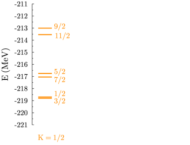
Figure 14: (Color online) Energy spectrum built from the expectation values $E^{JNZ}_{iK}$ for different values of $K$ obtained in the decomposition of the “axial state” as defined in Tab. 3.

Whenever a state $|\Phi\rangle$ can be decomposed into several $K$ components with given $J$, there is a necessary second step in the restoration of angular momentum that consists in the mixing of the projected wave functions with same $M$ but different $K$, i.e. the states $\big{\{}\hat{P}^{J}_{MK}|\Phi\rangle,K\in\llbracket-J,J\rrbracket\big{\}}$. It is only after this mixing that one obtains an orthogonal set of correlated states of given $J$ in the vector space $\text{span}(G|\Phi\rangle)$ that diagonalize the Hamiltonian and that are independent on the orientation of the reference state $|\Phi\rangle$. The effect of $K$ mixing sensitively depends on the properties of the state $|\Phi\rangle$ that is projected. It may be very mild or change drastically the energy spectrum at hand. In Figs. 14 and 15 we display the spectrum built based on the projected energies

$$E^{JNZ}_{iK}=\frac{\langle\Phi_{i}|\hat{H}\,\hat{P}^{J}_{KK}\,\hat{P}^{Z}\,\hat{P}^{N}|\Phi_{i}\rangle}{\langle\Phi_{i}|\hat{P}^{J}_{KK}\,\hat{P}^{Z}\,\hat{P}^{N}|\Phi_{i}\rangle}\,,$$ (168)

for three different states, considering only positive values of $K$ as the components with $\pm K$ are degenerate because of the $x$-signature imposed on all states $|\Phi_{i}\rangle$ considered throughout this Section. As explained in Sect. V.3, these pairs of states will contribute with weights of equal absolute value to the $K$-mixed states.

Figure 14 shows the energy spectrum for the “axial state” as defined in Tab. 3 that only has $K=\pm 1/2$ components. Applying the suitable transformation $\boldsymbol{W}^{J}_{\eta}$ as defined in Eq. (147) accomplishes the necessary $K$ mixing without the need to solve the GEP (154), and without changing the energy spectrum. In fact, this example illustrates a case that can also be described with the phenomenological Unified Model as defined in Refs. Bohr (1976); Rowe (1970); Bohr and Mottelson (1998); Ring and Schuck (1980) that is widely used to interpret rotational bands of odd-mass nuclei in terms of simple intrinsic configurations relying on the schematic picture of a single-particle state coupled to a deformed core. In the Unified Model, the treatment of the special case of rotational bands built on $k=1/2$ orbits requires the introduction of an additional $\Delta J=1$ Coriolis interaction with a so-called “decoupling parameter”, that in some cases pairwise switches the relative order of the energy levels compared to their usual scaling with $J(J+1)-K^{2}$, see also Ref. Ring et al. (1970). In an angular-momentum projected approach this effect is automatically described with a size that is entirely determined by the properties of the reference state, and the state used to prepare Fig. 14 is an example where the order of the states is indeed changed.

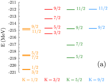
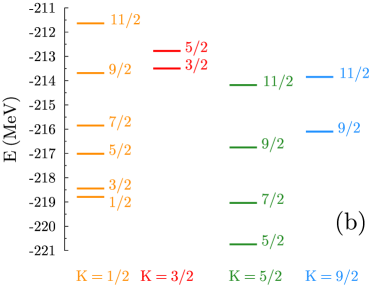
Figure 15: (Color online) Same as Fig. 14 for the decomposition states of the states $|\Phi_{a}\rangle$ (panel (a)) and $|\Phi_{b}\rangle$ (panel (b)) as defined in Tab. 4. The color of the levels indicates the value of $K$, whereas the labels next to the levels indicate the value of $J$.

label	$\langle\hat{Z}\rangle$	$\langle\hat{N}\rangle$	$(\beta_{2},\gamma)$	$\eta$	$p$	$\langle\hat{d}_{z}\rangle$	$\langle\hat{d}_{z}\rangle_{\text{axial}}$
a	12	13	$(0.60,14^{\circ})$	$-i$	1	0.65	0.50
b	12	13	$(0.47,24^{\circ})$	$-i$	1	1.82	2.50

Table 4: Characteristics of the quasiparticle vacua used to prepare Figs. 15 and 16.

For two other triaxial quasiparticle vacua, whose characteristics are given in Tab. 4, we plot in Fig. 15 the spectra of $(J,K)$ components up to $K=9/2$. Their respective decomposition in energy is quite different from the one of Fig. 14 and also among each other. These two states have non-vanishing components for each possible value of $|K|$ for given $J$. Without $K$ mixing, the levels of same $K$ but different $J$ do not necessarily form the usual pattern of a rotational band, which is again most obvious for $K=1/2$ components for which the order of levels is again pairwise switched as for the state discussed in Fig. 14. At low $J$, the decomposition of state $|\Phi_{\text{a}}\rangle$ in general energetically favors the band based on $K=1/2$ components and gives an excited band based on $K=5/2$. For state $|\Phi_{\text{b}}\rangle$ one finds the opposite. This dominance is a fingerprint of the single-particle configuration that has been self-consistently blocked. Although the final many-body state is not pure, i.e. many bands appear in its decomposition, the dominant component is usually energetically favored. The other bands based on higher $K$ components are rather similar.

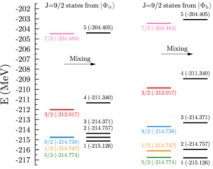
Figure 16: (Color online) Spectrum of $J=9/2$ states before and after $K$-mixing for the state $|\Phi_{\text{a}}\rangle$ and $|\Phi_{b}\rangle$ as defined in Tab. 4. The energies $E^{JNZ}_{iK}$ (168) of $K$ components are drawn in the same color code as used in Fig. 15, whereas energy levels after $K$ mixing are drawn in black. Note that the three lowest $K$ components of state $|\Phi_{\text{a}}\rangle$ are quasi-degenerate, such that their levels fall on top of each other on the scale of the plot.

Both states have the particularity that one finds near-degenerate $J=9/2$ components with different $K$ in their decomposition. In Fig. 16, we compare the energies of these $K$ components with the eigenvalues of the projected states after $K$-mixing. In the case of state $|\Phi_{\text{a}}\rangle$, we see that $K$-mixing has the effect of lifting the degeneracy of the three lowest states with $K=1/2$, $5/2$, and $9/2$, with one state visibly being lowered, another one being pushed up and the third staying in between as can be expected from the general principles of configuration mixing. The $K=3/2$ and $K=7/2$ components are also clearly mixed with the others. The fourth state in the spectrum is actually more shifted energetically than the first three states despite the $K=3/2$ component being more isolated. For the state $|\Phi_{\text{b}}\rangle$, the values of the diagonal matrix elements before mixing are more spread such that the diagonalisation does not change the global aspect of the spectrum. Nevertheless, the $K$-mixing still has an effect on the energies and even the highest energy state, well above the others, is changed. All other observables are also obviously affected by the $K$ mixing, which we will not discuss. In both cases, there are no redundant components in the decomposition after the transformation $\boldsymbol{W}^{J}_{\eta}$ as defined in Eq. (147) has been applied, such that one obtains five different $J=9/2$ states after $K$ mixing.

V.6.3 Projection of cranked states

The self-consistent cranking approach has been used for a long time to construct collective rotational bands in single-reference valence-space Ring et al. (1970) and EDF calculations Bonche et al. (1987). It can be motivated either as a self-consistent state in a rotating frame subject to Coriolis forces Thouless and Valatin (1962), or as the first-order approximation to a VAP on angular momentum Kamlah (1968); Beck et al. (1970); Villars and Schmeing-Rogerson (1971); Mang (1975); Islam et al. (1979), see also Sect. IV.1. The PAV on angular momentum of cranked Slater determinants and Bogoliubov quasiparticle vacua has been used in exploratory studies using valence-space Hamiltonians Hara et al. (1982), the BKN EDF Baye and Heenen (1984), the Gogny force Borrajo et al. (2015); Shimada et al. (2015); Egido et al. (2016), and the Skyrme EDF Zduńczuk et al. (2007, 2007), in some cases combined with further configuration mixing of states with different deformation and/or of states at different expectation value of angular momentum Egido et al. (2016).

Practically speaking, assuming a good $x$-signature, for states that are nearly axial around the $z$ axis, the self-consistent cranking approximation usually consists in adding an auxiliary condition on the expectation value of the form

$$\langle\hat{J}_{x}\rangle_{a(J_{c})}\equiv\langle\Phi_{a(J_{c})}|\hat{J}_{x}|\Phi_{a(J_{c})}\rangle=\sqrt{J_{c}(J_{c}+1)-K^{2}_{c}}\,,$$ (169)

during the minimization procedure of the state $|\Phi_{a(J_{c})}\rangle$ Ring et al. (1970); Beck et al. (1970); Ring et al. (1974); Ejiri and de Voigt (1989), where $J_{c}$ is the targeted angular momentum and $K_{c}$ is the assumed length of the component of angular momentum in $z$ direction, which depends on the characteristics of the blocked quasiparticles of the state $|\Phi_{a(J_{c})}\rangle$. We recall that when imposing $\langle\hat{P},\hat{R}_{x},\hat{S}^{\mathcal{T}}_{y}\rangle$ symmetry, only the angular momentum operator in $x$ direction can have non-zero expectation value, and $K_{c}$ is related to the $z$ component of the decoupling vector as defined above.

Because angular momentum changes sign under time reversal, the cranking constraint necessarily breaks the time-reversal invariance of the self-consistent procedure. The constraint (169) introduces a Coriolis interaction that in general acts differently on two nucleons in time-reversed single-particle states and thereby splits Kramers degeneracy. The reason is that one out of the two single-particle states has a component of angular momentum that is aligned with the cranking constrained, whereas the angular momentum of its time-reversed partner state is anti-aligned. If the cranking constraint is the only source of time-reversal breaking, which implies $K=0$ in Eq. (169), then cranking a state to $-\langle\hat{J}_{x}\rangle_{a(J_{c})}$ generates the time-reversed of the state that is obtained when cranking to $+\langle\hat{J}_{x}\rangle_{a(J_{c})}$, meaning that both states are equivalent as discussed in Sect. V.4.

When cranking a blocked quasiparticle vacuum, however, one can always construct two such pairs of non-equivalent solutions: one for which one blocks a quasiparticle whose measurable $x$-component of angular-momentum is aligned with the direction of the cranking constraint, and one for which one blocks its time-reversed partner that is anti-aligned. The resulting many-body states cannot be transformed one into the other by time-reversal and will in general have slightly different total energy and and other observables Ring et al. (1974). For reasons elaborated for example in Ref. Ring et al. (1970, 1974); Mang (1975) and recalled in what follows, it is customary to construct states cranked to $J_{c}=1/2$, $5/2$, $9/2$, $13/2$, …by blocking a single-particle level with $x$-signature $\eta_{a}=-i$, whereas states cranked to $J_{c}=3/2$, $7/2$, $11/2$, $15/2$, …are constructed by blocking a single-particle level with $\eta_{a}=+i$. These states are usually grouped into two different signature-partner bands, for which one often finds experimentally that the levels in one band do not fall exactly in between those in the other, but are slightly shifted Szymanski (1984); Ejiri and de Voigt (1989), an effect that is in general also found in cranked HFB calculations.

In order to illustrate this effect, we display in Fig. 17 the summed weight of the components with given $J$

$$\Xi^{J}=\sum_{K=-J}^{J}N^{J}_{KK}\,,$$ (170)

obtained when projecting two one-quasiparticle states of ²⁵Mg obtained by blocking quasiparticles in (originally time-reversed) partner orbits of opposite $x$-signature $\eta_{a}=+i$ and $\bar{\eta}_{a}=-i$, and which are cranked to different values of $J_{c}$ as defined in Eq. (169). These states are constructed in the same way as those discussed above.

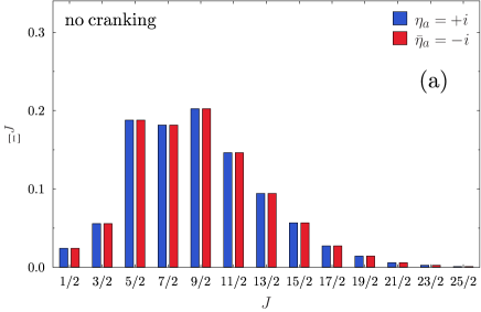
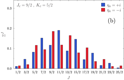
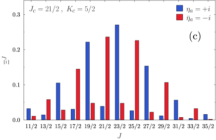
Figure 17: (Color online) Summed weight $\Xi^{J}$ as defined in Eq. (170) of components with given $J$ projected out from one-quasiparticle states for ²⁵Mg obtained by blocking single particles in originally time-reversed partner states of opposite $x$-signature $\eta$, and cranked to different values of $J_{c}$.

As can be seen, in the absence of cranking constraint (panel (a)) the two distribution of the weights $\Xi^{J}$ are equal, up to numerical accuracy, which follows from the discussion in Sect. V.4. With increasing value of the constrained angular momentum $J_{c}$ (panels (b) and (c)), the two distributions become different, with every second component becoming much smaller. In the limit of high collective angular momentum $J_{c}\gg K_{c}$ the two blocked states have a very different decomposition, and one then finds a distribution of components that mirrors the rules for the selection of the blocked single-particle levels mentioned above: cranked one-quasiparticle states $|\Phi_{a(J_{c})}\rangle$ with $x$-signature $\eta_{a(J_{c})}=+i$ are dominated by components with $J=3/2$, $7/2$, $11/2$, $15/2$, etc, whereas one-quasiparticle states with $x$-signature $\eta_{a(J_{c})}=-i$ are dominated by components with $J=1/2$, $5/2$, $9/2$, $13/2$, etc. We remark that this selection rule can also be understood using the Kamlah expansion Kamlah (1968) at large spin (see Ref. Bally (2014) for more details).

Finally, we notice that as we increase the value of the constraint, the distribution of components move to larger values of $J$, and becomes wider. For the two cranked states, the distribution of the components is peaked near the cranked angular momentum, which is not always the case Islam et al. (1979); Baye and Heenen (1984); Zduńczuk et al. (2007, 2007).

Figure 18: (Color online) Projected energies, as defined in Eq. (171), of yrast states projected from two one-quasiparticle states for ²⁵Mg obtained from blocking two originally time-reversed partners of opposite $x$-signature $\eta_{a}$ cranked to different values of $J_{c}$ as indicated.

The effect of cranking on blocked one-quasiparticle states can also be seen on the energies of the symmetry-restored states

$$E^{JNZ}_{a\epsilon(J_{c})}=\langle\Psi_{a\epsilon(J_{c})}^{JMNZ}|\hat{H}|\Psi_{a\epsilon(J_{c})}^{JMNZ}\rangle\,,$$ (171)

displayed in Fig. 18 for yrast states obtained when cranking the one-quasiparticle states to different values of $J_{c}$. The cranked states used to prepare this figure have the same slightly triaxial shape as the states used to prepare Fig. 17, but cover also intermediate values of the cranked angular momentum $J_{c}$. First, we observe that in the absence of a cranking constraint the energies of the projected states built from the states of opposite signatures are strictly equal for a given $J$, which is expected as the two states are in that case connected by time-reversal. By contrast, when a cranking constraint is added during the minimization, the projected energies for given $J$ split. Their difference varies greatly depending on $J$ and $J_{c}$. For all values of $J$ the cranked states always give lower projected energies than the non-cranked ones, with the gain in energy usually increasing with $J$ as already found earlier Borrajo et al. (2015); Shimada et al. (2015); Egido et al. (2016); Zduńczuk et al. (2007, 2007). This confirms that self-consistent cranking optimizes the states for subsequent projection on high angular momentum as should be expected from an approximation to a VAP calculation. But for the values of cranked and projected angular momenta covered by Fig. 18, we do not observe any clear pattern indicating which $x$-signature will be favored energetically.

VI Summary and Conclusions

The quantum-number projection technique is a powerful tool that permits to build symmetry-adapted wave functions starting from any arbitrary many-body reference state. In addition, when defined as the diagonalization of the nuclear Hamiltonian in the subspace spanned by the set of all rotated states (built by rotating the initial reference state in all possible ways) as elaborated in Section II, the method provides a procedure to grasp correlation energy that is absent in a symmetry-breaking calculation The eigenstates thus obtained represent variationally optimal wave functions (in this subspace) that respect the symmetries of the problem and therefore can be used to compute unambiguously the expectation values of observables of interest. In particular, the projection restores selection rules for the matrix elements of tensor operators.

In Sections III and IV, we illustrated the method in the case of particle-number and angular-momentum projections. In each case, we presented the general principles of the projection as well as the practical aspects of its numerical implementation. While the group $U(1)$ associated with a good number particles is abelian, the group $SU(2)$ associated with a good angular momentum is not, which makes the latter projection much more involved. Nevertheless, it is possible in both cases to use efficient numerical discretizations of the integrals over group elements. When a sufficiently large number of discretization points is used, the integration is performed exactly up to the numerical noise.

We have limited our discussion to these two continuous symmetries. Another case of interest not addressed here is the breaking and restoration of parity Egido and Robledo (1991), which from a formal and practical point of view is much simpler and straightforward: as it is a discrete abelian symmetry, parity projection of a reflection-symmetry-breaking state always corresponds to the mixing of exactly two states, the original one and its parity-inverted image. Their superposition span a vector space of dimension two that is the direct product of two one-dimensional subspaces corresponding to the irreps with parity $\pm 1$. As a consequence, there are no questions about the discretization of the numerical representation of the parity projection operator in order to achieve optimal convergence.

Finally, in section V, we gave formal results that permit a great deal of simplifications when dealing with reference states that have the symmetry properties of the subgroup $\langle\hat{P},\hat{R}_{x},\hat{S}^{\mathcal{T}}_{y}\rangle$ of the group $D_{2h}^{TD}$, often employed in nuclear physics to describe collective phenomena in axially and triaxially deformed nuclei. For this class of states, we derived the most general expressions that can be applied to any reference state, whatever its number parity or the angular momentum considered.

Up to now, the projection method has been used extensively within multi-reference formalism based on Slater determinants and Bogoliubov quasiparticle vacua, either using valence-space Hamiltonians or energy density functionals, to tackle a large variety of phenomena Bender et al. (2003); Egido (2016); Robledo et al. (2018); Sheikh et al. (2019). But there are also new ongoing developments to design ab-initio schemes that integrate symmetry restoration as one of their fundamental principles Duguet (2014); Duguet and Signoracci (2017); Hermes et al. (2017); Qiu et al. (2017, 2019); Yao et al. (2020b). For that reason, we precise that although we illustrated our discussion making use of Bogoliubov quasiparticle reference states, most of the results presented here can be directly carried over to more general types of symmetry-breaking reference states.

Appendix A Discretizations for particle-number projection

In Sec. III, we introduced a discretized projection operator for particle-number projection based on the original idea by Fomenko Fomenko (1970). Actually, there exist other choices that behave similarly but differ by the position of the quadrature points in the interval $[0,\pi]$. Indeed, choosing $\alpha\in[0,1]$ one defines the general discretized projection operator

$$\hat{\mathbb{P}}^{N_{0}}_{\alpha,M_{\varphi}}\equiv\frac{1}{M_{\varphi}}\,\sum_{m=1}^{M_{\varphi}}e^{-\text{i}\pi\frac{m-\alpha}{M_{\varphi}}(\hat{N}-N_{0})}\,.$$ (172)

All the operators corresponding to different values of $\alpha$ have in common that two consecutive angles are always separated by a step of $\pi/{M_{\varphi}}$, with the main difference being the position of the first angle. In this section we will analyze their action on a given wave function, focusing in particular on four specific values of $\alpha$. For the sake of keeping the discussion simple, we will consider only one generic particle species $N$ without any loss of generality.

The four possible choices for the discretized projection operator we will focus on are

$$\hat{\mathbb{P}}^{N_{0}}_{1,M_{\varphi}} \equiv\frac{1}{M_{\varphi}}\,\sum_{n=1}^{M_{\varphi}}e^{-\text{i}\pi\frac{n-1}{M_{\varphi}}(\hat{N}-N_{0})}\,,$$ (173)

$$\hat{\mathbb{P}}^{N_{0}}_{1/2,M_{\varphi}} \equiv\frac{1}{M_{\varphi}}\,\sum_{n=1}^{M_{\varphi}}e^{-\text{i}\pi\frac{n-\frac{1}{2}}{M_{\varphi}}(\hat{N}-N_{0})}\,,$$ (174)

$$\hat{\mathbb{P}}^{N_{0}}_{1/4,M_{\varphi}} \equiv\frac{1}{M_{\varphi}}\,\sum_{n=1}^{M_{\varphi}}e^{-\text{i}\pi\frac{n-\frac{1}{4}}{M_{\varphi}}(\hat{N}-N_{0})}\,,$$ (175)

$$\hat{\mathbb{P}}^{N_{0}}_{3/4,M_{\varphi}} \equiv\frac{1}{M_{\varphi}}\,\sum_{n=1}^{M_{\varphi}}e^{-\text{i}\pi\frac{n-\frac{3}{4}}{M_{\varphi}}(\hat{N}-N_{0})}\,,$$ (176)

where $\hat{\mathbb{P}}^{N_{0}}_{1,M_{\varphi}}$ is the standard one used in the core of the text.

Although they are otherwise very similar, the first of these discretized operators (173) has the practical advantage that it reduces to the identity operator when taking $M_{\varphi}=1$. By contrast, the third and fourth discretized operators never require the evaluation of the angle $\frac{\pi}{2}$ that might become numerically problematic in pure particle-number projection Anguiano et al. (2001), see also Sect. III.6. However, this problem can be avoided anyway by taking an odd number of points $M_{\varphi}$ for (173), respectively an even value of $M_{\varphi}$ for (174). In addition, when combined with other projections or a configuration mixing calculation the problem might appear at any gauge angle, not just $\frac{\pi}{2}$.

We will now analyze the action of operator $\hat{\mathbb{P}}^{N_{0}}_{\alpha,M_{\varphi}}$ acting on a reference state $|\Phi\rangle$ that is an eigenstate of number parity with an eigenvalue compatible with $N_{0}$, i.e. $\pi_{n}=(-)^{N_{0}}$. Using the decomposition (56) of $|\Phi\rangle$, we obtain that

$$\hat{\mathbb{P}}^{N_{0}}_{\alpha,M_{\varphi}}|\Phi\rangle=\sum_{N_{1}\geq 0}c^{N_{1}}\Bigg{(}\frac{1}{{M_{\varphi}}}\sum_{m=1}^{{M_{\varphi}}}e^{-\text{i}\pi\frac{m-\alpha}{{M_{\varphi}}}(N_{1}-N_{0})}\Bigg{)}|\Psi^{N_{1}}\rangle\,.$$ (177)

The factor

$$\frac{1}{{M_{\varphi}}}\sum_{m=1}^{{M_{\varphi}}}e^{-\text{i}\pi\frac{m-\alpha}{{M_{\varphi}}}(N_{1}-N_{0})}$$

on the r.h.s. of Eq. (177) is a geometric progression, i.e. a sum of the type $\sum_{k=i}^{j}\,a\,r^{k}$, with $r$ being the common ratio and $a$ the scale factor. Depending on the value of $r$, the result of a geometric progression can be expressed in a closed form as

$$\sum_{k=i}^{j}\,a\,r^{k}=\left\{\begin{array}[]{cc}a\,(j-i+1)&\text{if }r=1\,,\\ &\\ a\,\frac{r^{i}-r^{j+1}}{1-r}&\text{if }r\neq 1\,.\end{array}\right.$$

For the discretized projection operator $\hat{\mathbb{P}}^{N_{0}}_{\alpha,M_{\varphi}}$, we have

$$\begin{split}i&=1\,,\\ j&=M_{\varphi}\,,\\ r&=e^{-\text{i}\pi\frac{1}{{M_{\varphi}}}(N_{1}-N_{0})}\,,\\ a&=\frac{e^{+\text{i}\pi\frac{\alpha}{M_{\varphi}}(N_{1}-N_{0})}}{{M_{\varphi}}}\,.\end{split}$$

The case $r=1$ is realized if and only if $N_{1}=N_{0}+2\ell{M_{\varphi}}$ with $\ell\in\mathbb{Z}$. For those values of $N_{1}$, one thus obtains

$$\begin{split}\hat{\mathbb{P}}^{N_{0}}_{\alpha,M_{\varphi}}|\Psi^{N_{1}}\rangle&=\frac{e^{+\text{i}2\pi\alpha\ell}}{M_{\varphi}}\,\big{(}M_{\varphi}-1+1\big{)}\,|\Psi^{N_{1}}\rangle\\ &=e^{+\text{i}2\pi\alpha\ell}\,|\Psi^{N_{1}}\rangle\,.\end{split}$$ (178)

For any other value of $N_{1}$, one obtains instead

$$\begin{split}\hat{\mathbb{P}}^{N_{0}}_{\alpha,M_{\varphi}}|\Psi^{N_{1}}\rangle&=a\frac{1-e^{-\text{i}\pi(N_{1}-N_{0})}}{1-e^{-\text{i}\pi\frac{1}{{M_{\varphi}}}(N_{1}-N_{0})}}\,|\Psi^{N_{1}}\rangle\\ &=0\,,\end{split}$$ (179)

where we have used that $|\Phi\rangle$ is an eigenstate of number parity, such that we always have the relation $N_{1}=N_{0}+2n$, $n\in\mathbb{Z}$, for the components in (56), which implies that $1-e^{-\text{i}\pi(N_{1}-N_{0})}=0$. But note that this is true if and only if the state $|\Phi\rangle$ has a number parity equal to $(-)^{N_{0}}$, hence the assumption made earlier.

To summarize, by applying $\hat{\mathbb{P}}^{N_{0}}_{\alpha,M_{\varphi}}$ on $|\Phi\rangle$, we remove all components with $N_{1}\neq N_{0}+2\ell{M_{\varphi}},\,\ell\in\mathbb{Z}$,

$$\begin{split}\hat{\mathbb{P}}^{N_{0}}_{\alpha,M_{\varphi}}|\Phi\rangle&=\sum_{\ell\in\mathbb{Z}}e^{+\text{i}2\pi\alpha\ell}\,c^{N_{0}+2\ell M_{\varphi}}\,|\Psi^{N_{0}+2\ell M_{\varphi}}\rangle\\ &\equiv\sum_{\ell\in\mathbb{Z}}\sum_{N_{1}\geq 0}e^{+\text{i}2\pi\alpha\ell}\,c^{N_{1}}\,|\Psi^{N_{1}}\rangle\,\delta_{N_{1}N_{0}+2\ell M_{\varphi}}\,.\end{split}$$ (180)

We can notice in particular that the discretized projection operator exhibits a periodicity of $2M_{\varphi}$, i.e.

$$\forall\,\ell_{1}\in\mathbb{Z},\,\hat{\mathbb{P}}^{N_{0}+2\ell M_{\varphi}}_{\alpha,M_{\varphi}}|\Phi\rangle=e^{-\text{i}2\pi\alpha\ell_{1}}\hat{\mathbb{P}}^{N_{0}}_{\alpha,M_{\varphi}}|\Phi\rangle\,.$$ (181)

As a consequence, the projection on any particle number $N_{2}$ that is such that $N_{2}=N_{0}+2\ell_{1}M_{\varphi}$, $\ell_{1}\in\mathbb{Z}$, will yield same result, up to a phase, as the projection on $N_{0}$, even if the component with $N_{2}$ particles is not present in the wave function that is projected. In particular, if $\alpha\ell_{1}\in\mathbb{Z}$, the projected wave functions are strictly equal.

Replacing the value of $\alpha$, we directly obtain the action of the four discretization operators of interest

$$\hat{\mathbb{P}}_{1,M_{\varphi}}^{N_{0}}|\Phi\rangle =\sum_{l\in\mathbb{Z}} c^{N_{0}+2\ell M_{\varphi}}\,|\Psi^{N_{0}+2lM_{\varphi}}\rangle\,,$$ (182)

$$\hat{\mathbb{P}}_{1/2,M_{\varphi}}^{N_{0}}|\Phi\rangle =\sum_{l\in\mathbb{Z}} (-)^{\ell} c^{N_{0}+2\ell M_{\varphi}}\,|\Psi^{N_{0}+2lM_{\varphi}}\rangle\,,$$ (183)

$$\hat{\mathbb{P}}_{1/4,M_{\varphi}}^{N_{0}}|\Phi\rangle =\sum_{l\in\mathbb{Z}} (\text{i})^{\ell} c^{N_{0}+2\ell M_{\varphi}}\,|\Psi^{N_{0}+2lM_{\varphi}}\rangle\,,$$ (184)

$$\hat{\mathbb{P}}_{3/4,M_{\varphi}}^{N_{0}}|\Phi\rangle =\sum_{l\in\mathbb{Z}} (-\text{i})^{\ell}\, c^{N_{0}+2\ell M_{\varphi}}\,|\Psi^{N_{0}+2lM_{\varphi}}\rangle\,.$$ (185)

As previously discussed, such discretized projection operators can only be used for states with a number parity equal to $(-)^{N_{0}}$. It is straightforward to define more general discretized projection operators that can be used regardless of the number parity of the state to be projected by simply replacing the factor $\pi$ in the exponential of any of these operators by a factor $2\pi$. Indeed, in that case we can lift the number parity condition for Eq. (179) as for any values of $N_{0}$ and $N_{1}$, we always have in the numerator: $1-e^{-\text{i}2\pi(N_{1}-N_{0})}=0$. But using the same rationale as above, it is straightforward to derive that such a discretized operators select out of the reference state all the components with $N_{1}=N_{0}+l{M_{\varphi}},\,l\in\mathbb{Z}$. Consequently, from a convergence point of view, these operators are less effective than the ones defined with a factor $\pi$. More precisely, the periodicity of the generalized operators being twice as small as the one of the operators defined in Eqs. (173)-(176), this would require a number of points ${M_{\varphi}}$, i.e. a number of rotations over gauge angles to be performed, twice as large to remove the same number of undesired components in the superposition (56).

References

- Henley (1996) E. M. Henley, ed., Symmetries Throughout the Sciences (Proc. Natl. Acad. Sci. USA 93, no. 25, 1996).
- Caulton (2015) A. Caulton, Studies in History and Philosophy of Science Part B: Studies in History and Philosophy of Modern Physics 52, 153 (2015).
- Noether (1918) E. Noether, Nachrichten von der Gesellschaft der Wissenschaften zu Göttingen, Mathematisch-Physikalische Klasse 1918, 235 (1918).
- Kosmann-Schwarzbach (2011) Y. Kosmann-Schwarzbach, The Noether Theorems. Invariance and Conservation Laws in the Twentieth Century (Springer-Verlag, New York, 2011).
- Wigner (1959) E. Wigner, Group Theory and its Applications to the Quantum Mechanics of Atomic Spectra (Academic Press Inc., 1959).
- Hamermesh (1962) H. Hamermesh, Group Theory and its applications to Physical problems (Dover Publications Inc., 1962).
- Tinkham (1992) M. Tinkham, Group Theory and Quantum Mechanics (Dover Publications Inc., 1992).
- McWeeny (2002) R. McWeeny, An Introduction to Group Theory and its Applications (Dover Publications Inc., 2002).
- Löwdin (1967) P. Löwdin, Rev. Mod. Phys. 39, 259 (1967).
- Lykos and Pratt (1963) P. Lykos and G. W. Pratt, Rev. Mod. Phys. 35, 496 (1963).
- Strocchi (2005) F. Strocchi, Symmetry Breaking, Lecture Notes in Physics, Vol. 643 (Springer-Verlag, Berlin, Heidelberg, 2005).
- Bohr (1976) Å. Bohr, Rev. Mod. Phys. 48, 365 (1976).
- Rowe (1970) D. J. Rowe, Nuclear Collective Motion: Models and Theory (Methuen, London, 1970).
- Bohr and Mottelson (1998) Å. Bohr and B. R. Mottelson, Nuclear structure, volume II (World Scientific Publishing, Singapore, 1998).
- Ring and Schuck (1980) P. Ring and P. Schuck, The Nuclear Many-Body Problem (Springer-Verlag, New York, 1980).
- Frauendorf (2001) S. Frauendorf, Rev. Mod. Phys. 73, 463 (2001).
- Peierls and Yoccoz (1957) R. E. Peierls and J. Yoccoz, Proc. Phys. Soc. London A 70, 381 (1957).
- Blaizot and Ripka (1986) J.-P. Blaizot and G. Ripka, Quantum Theory of Finite Systems (MIT Press, Cambridge, Massachusetts, 1986).
- MacDonald (1970) N. MacDonald, Advances in Phys. 19, 371 (1970).
- Sheikh and Ring (2000) J. A. Sheikh and P. Ring, Nucl. Phys. A 665, 71 (2000).
- Kanada-En’yo (1998) Y. Kanada-En’yo, Phys. Rev. Lett. 81, 5291 (1998).
- Gao et al. (2015) Z.-C. Gao, M. Horoi, and Y. S. Chen, Phys. Rev. C 92, 064310 (2015).
- Anguiano et al. (2001) M. Anguiano, J. L. Egido, and L. M. Robledo, Nucl. Phys. A 696, 467 (2001).
- Egido (2016) J. L. Egido, Phys. Scri. 91, 073003 (2016).
- Rodríguez et al. (2005) T. R. Rodríguez, J. L. Egido, and L. M. Robledo, Phys. Rev. C 72, 064303 (2005).
- Bender et al. (2006) M. Bender, G. F. Bertsch, and P.-H. Heenen, Phys. Rev. C 73, 034322 (2006).
- Ripka (1968) G. Ripka, in Advances in Nuclear Physics, Vol. 1, edited by M. Baranger and E. Vogt (Springer, Boston, MA., 1968) p. 183.
- Mang (1975) H. J. Mang, Phys. Rep. 18, 327 (1975).
- Schmid (2004) K. W. Schmid, Prog. Part. Nucl. Phys. 52, 565 (2004).
- Otsuka et al. (2001) T. Otsuka, M. Honma, T. Mizusaki, N. Shimizu, and Y. Utsuno, Prog. in Part. Nucl. Phys. 47, 319 (2001).
- Shimizu et al. (2012) N. Shimizu, T. Abe, Y. Tsunoda, Y. Utsuno, T. Yoshida, T. Mizusaki, M. Honma, and T. Otsuka, Progress of Theoretical and Experimental Physics 2012 (2012), 01A205.
- Hara and Sun (1995) K. Hara and Y. Sun, Int. J. Mod. Phys. E 04, 637 (1995).
- Sun (2016) Y. Sun, Phys. Scr. 91, 043005 (2016).
- Bender et al. (2004a) M. Bender, P. Bonche, T. Duguet, and P.-H. Heenen, Phys. Rev. C 69, 064303 (2004a).
- Nikšić et al. (2006) T. Nikšić, D. Vretenar, and P. Ring, Phys. Rev. C 74, 064309 (2006).
- Kimura (2007) M. Kimura, Phys. Rev. C 75, 041302(R) (2007).
- Bender and Heenen (2008) M. Bender and P.-H. Heenen, Phys. Rev. C 78, 024309 (2008).
- Rodríguez and Egido (2010) T. R. Rodríguez and J. L. Egido, Phys. Rev. C 81, 064323 (2010).
- Rodríguez-Guzman et al. (2012) R. Rodríguez-Guzman, L. M. Robledo, and P. Sarriguren, Phys. Rev. C 86, 034336 (2012).
- Yao et al. (2011) J. M. Yao, H. Mei, H. Chen, J. Meng, P. Ring, and D. Vretenar, Phys. Rev. C 83, 014308 (2011).
- Satuła et al. (2010) W. Satuła, J. Dobaczewski, W. Nazarewicz, and M. Rafalski, Phys. Rev. C 81, 054310 (2010).
- Bally et al. (2014) B. Bally, B. Avez, M. Bender, and P.-H. Heenen, Phys. Rev. Lett. 113, 162501 (2014).
- Borrajo et al. (2015) M. Borrajo, T. R. Rodríguez, and J. L. Egido, Phys. Lett. B 746, 341 (2015).
- Rodríguez et al. (2015) T. R. Rodríguez, A. Arzhanov, and G. Martínez-Pinedo, Phys. Rev. C 91, 044315 (2015).
- Egido et al. (2016) J. L. Egido, M. Borrajo, and T. R. Rodríguez, Phys. Rev. Lett. 116, 052502 (2016).
- Robledo et al. (2018) L. M. Robledo, T. R. Rodríguez, and R. R. Rodríguez-Guzmán, J. Phys. G 46, 013001 (2018).
- Shimada et al. (2015) M. Shimada, S. Tagami, and Y. R. Shimizu, Progress of Theoretical and Experimental Physics 2015 (2015), 063D02.
- Ushitani et al. (2019) M. Ushitani, S. Tagami, and Y. R. Shimizu, Phys. Rev. C 99, 064328 (2019).
- Bender et al. (2019) M. Bender, N. Schunck, J.-P. Ebran, and T. Duguet, in Energy Density Functional Methods for Atomic Nuclei, 2053-2563, edited by N. Schunck (IOP Publishing, 2019) pp. 3–1 to 3–78.
- Somà et al. (2013) V. Somà, C. Barbieri, and T. Duguet, Phys. Rev. C 87, 011303 (2013).
- Hergert et al. (2014) H. Hergert, S. K. Bogner, T. D. Morris, S. Binder, A. Calci, J. Langhammer, and R. Roth, Phys. Rev. C 90, 041302 (2014).
- Signoracci et al. (2015) A. Signoracci, T. Duguet, G. Hagen, and G. R. Jansen, Phys. Rev. C 91, 064320 (2015).
- Neff and Feldmeier (2008) T. Neff and H. Feldmeier, Eur. Phys. J. Special Topics 156, 69 (2008).
- Duguet (2014) T. Duguet, J. Phys. G 42, 025107 (2014).
- Hergert et al. (2016) H. Hergert, S. Bogner, T. Morris, A. Schwenk, and K. Tsukiyama, Phys. Rep. 621, 165 (2016).
- Duguet and Signoracci (2017) T. Duguet and A. Signoracci, J. Phys. G 44, 015103 (2017).
- Qiu et al. (2017) Y. Qiu, T. M. Henderson, J. Zhao, and G. E. Scuseria, The Journal of Chemical Physics 147, 064111 (2017).
- Qiu et al. (2019) Y. Qiu, T. M. Henderson, T. Duguet, and G. E. Scuseria, Phys. Rev. C 99, 044301 (2019).
- Yao et al. (2020a) J. M. Yao, B. Bally, J. Engel, R. Wirth, T. R. Rodríguez, and H. Hergert, Phys. Rev. Lett. 124, 232501 (2020a).
- Rodríguez-Guzmán and Schmid (2004a) R. R. Rodríguez-Guzmán and K. W. Schmid, Eur. Phys. J. A 19, 45 (2004a).
- Rodríguez-Guzmán and Schmid (2004b) R. R. Rodríguez-Guzmán and K. W. Schmid, Eur. Phys. J. A 19, 61 (2004b).
- Dobaczewski et al. (2000a) J. Dobaczewski, J. Dudek, S. G. Rohoziński, and T. R. Werner, Phys. Rev. C 62, 014310 (2000a).
- Dobaczewski et al. (2000b) J. Dobaczewski, J. Dudek, S. G. Rohoziński, and T. R. Werner, Phys. Rev. C 62, 014311 (2000b).
- Dönau (1998) F. Dönau, Phys. Rev. C 58, 872 (1998).
- Dobaczewski et al. (2007) J. Dobaczewski, M. V. Stoitsov, W. Nazarewicz, and P.-G. Reinhard, Phys. Rev. C 76, 054315 (2007).
- Robledo (2007) L. M. Robledo, Int. J. Mod. Phys. E 16, 337 (2007).
- Lacroix et al. (2009) D. Lacroix, T. Duguet, and M. Bender, Phys. Rev. C 79, 044318 (2009).
- Bender et al. (2009) M. Bender, T. Duguet, and D. Lacroix, Phys. Rev. C 79, 044319 (2009).
- Duguet et al. (2009) T. Duguet, M. Bender, K. Bennaceur, D. Lacroix, and T. Lesinski, Phys. Rev. C 79, 044320 (2009).
- Robledo (2010) L. M. Robledo, J. Phys. G 37, 064020 (2010).
- Satuła and Dobaczewski (2014) W. Satuła and J. Dobaczewski, Phys. Rev. C 90, 054303 (2014).
- Rowe and Wood (2010) D. J. Rowe and J. L. Wood, Fundamentals of Nuclear Models (World Scientific Publishing, Singapore, 2010).
- Peter and Weyl (1927) F. Peter and H. Weyl, Math. Ann. 97, 737 (1927).
- Sheikh et al. (2019) J. A. Sheikh, J. Dobaczewski, P. Ring, L. M. Robledo, and C. Yannouleas, “Symmetry restoration in mean-field approaches,” (2019), arXiv:1901.06992 [nucl-th] .
- Egido and Ring (1982) J. Egido and P. Ring, Nucl. Phys. A 383, 189 (1982).
- Maqbool et al. (2011) I. Maqbool, J. A. Sheikh, P. A. Ganai, and P. Ring, J. Phys. G 38, 045101 (2011).
- Bender et al. (2003) M. Bender, P.-H. Heenen, and P.-G. Reinhard, Rev. Mod. Phys. 75, 121 (2003).
- Jiao and Johnson (2019) C. Jiao and C. W. Johnson, Phys. Rev. C 100 (2019).
- Robledo (2009) L. M. Robledo, Phys. Rev. C 79, 021302 (2009).
- Avez and Bender (2012) B. Avez and M. Bender, Phys. Rev. C 85, 034325 (2012).
- Mizusaki et al. (2018) T. Mizusaki, M. Oi, and N. Shimizu, Phys. Lett. B 779, 237 (2018).
- Carlsson and Rotureau (2020) B. G. Carlsson and J. Rotureau, “A new and practical formulation for overlaps of bogoliubov vacua,” (2020), arXiv:2010.08459 [nucl-th] .
- Bally and Duguet (2018) B. Bally and T. Duguet, Phys. Rev. C 97, 024304 (2018).
- Hermes et al. (2017) M. R. Hermes, J. Dukelsky, and G. E. Scuseria, Phys. Rev. C 95, 064306 (2017).
- Yao et al. (2020b) J. M. Yao, B. Bally, J. Engel, R. Wirth, T. R. Rodríguez, and H. Hergert, Phys. Rev. Lett. 124, 232501 (2020b).
- Bonche et al. (1990) P. Bonche, J. Dobaczewski, H. Flocard, P.-H. Heenen, and J. Meyer, Nucl. Phys. A510, 466 (1990).
- Mang et al. (1966) H. J. Mang, J. O. Rasmussen, and M. Rho, Phys. Rev. 141, 941 (1966).
- Nogami (1964) Y. Nogami, Phys. Rev. 134, B313 (1964).
- Pradhan et al. (1973) H. C. Pradhan, Y. Nogami, and J. Law, Nucl. Phys. A201, 357 (1973).
- Bender et al. (2000) M. Bender, K. Rutz, P. G. Reinhard, and J. A. Maruhn, Eur. Phys. J A8, 59 (2000).
- Valor et al. (2000a) A. Valor, J. L. Egido, and L. M. Robledo, Nucl. Phys. A665, 46 (2000a).
- Kamlah (1968) A. Kamlah, Z. Phys. 216, 52 (1968).
- Valor et al. (2000b) A. Valor, J. L. Egido, and L. M. Robledo, Nucl. Phys. A671, 189 (2000b).
- Flocard and Onishi (1997) H. Flocard and N. Onishi, Ann. Phys. 254, 275 (1997).
- Wang et al. (2014) X. B. Wang, J. Dobaczewski, M. Kortelainen, L. F. Yu, and M. V. Stoitsov, Phys. Rev. C 90, 014312 (2014).
- Dietrich et al. (1964) K. Dietrich, H. J. Mang, and J. H. Pradal, Phys. Rev. 135, B22 (1964).
- Braun and von Delft (1998) F. Braun and J. von Delft, Phys. Rev. Lett. 81, 4712 (1998).
- Sheikh et al. (2002) J. A. Sheikh, P. Ring, E. Lopes, and R. Rossignoli, Phys. Rev. C 66, 044318 (2002).
- Hupin and Lacroix (2012) G. Hupin and D. Lacroix, Phys. Rev. C 86, 024309 (2012).
- Hara et al. (1982) K. Hara, A. Hayashi, and P. Ring, Nucl. Phys. A385, 14 (1982).
- Perez-Martin and Robledo (2008) S. Perez-Martin and L. M. Robledo, Phys. Rev. C 78, 014304 (2008).
- Goodman (1981) A. L. Goodman, Nucl. Phys. A 352, 30 (1981).
- Tanabe and Nakada (2005) K. Tanabe and H. Nakada, Phys. Rev. C 71, 024314 (2005).
- Bally (2014) B. Bally, Description of odd-mass nuclei by multi-reference energy density functional methods, Ph.D. thesis, Université de Bordeaux (2014).
- Vaquero et al. (2013) N. L. Vaquero, T. R. Rodríguez, and J. L. Egido, Phys. Rev. Lett. 111, 142501 (2013).
- Romero et al. (2019) A. M. Romero, J. Dobaczewski, and A. Pastore, Phys. Lett. B 795, 177 (2019).
- Bayman (1960) B. F. Bayman, Nucl. Phys. 15, 33 (1960).
- Frank and Van Isacker (1982) A. Frank and P. Van Isacker, Phys. Rev. C 26, 1661 (1982).
- Lacroix and Hupin (2010) D. Lacroix and G. Hupin, Phys. Rev. B 82, 144509 (2010).
- Hupin et al. (2011) G. Hupin, D. Lacroix, and M. Bender, Phys. Rev. C 84, 014309 (2011).
- Fomenko (1970) V. N. Fomenko, J. Phys. A 3, 8 (1970).
- Samyn et al. (2004) M. Samyn, S. Goriely, M. Bender, and J. M. Pearson, Phys. Rev. C 70, 044309 (2004).
- Schmid and Grümmer (1987) K. W. Schmid and F. Grümmer, Rep. Prog. Phys. 50, 731 (1987).
- Duguet et al. (2020) T. Duguet, B. Bally, and A. Tichai, “Zero-pairing limit of Hartree-Fock-Bogoliubov reference states,” (2020), arXiv:2006.02871 [nucl-th] .
- Duguet and Ryssens (2020) T. Duguet and W. Ryssens, Phys. Rev. C 102, 044328 (2020).
- Angeli and Marinova (2015) I. Angeli and K. P. Marinova, J. Phys. G 42, 055108 (2015).
- Beck et al. (1970) R. Beck, H. J. Mang, and P. Ring, Z. Physik 231, 26 (1970).
- Villars and Schmeing-Rogerson (1971) F. Villars and N. Schmeing-Rogerson, Ann. Phys. (NY) 63, 443 (1971).
- Wong (1975) C. W. Wong, Phys. Rep. 15, 283 (1975).
- Islam et al. (1979) S. Islam, H. J. Mang, and P. Ring, Nucl. Phys. A 326, 161 (1979).
- Thouless and Valatin (1962) D. J. Thouless and J. G. Valatin, Nucl. Phys. 31, 211 (1962).
- Peierls and Thouless (1962) R. E. Peierls and D. J. Thouless, Nucl. Phys. 38, 154 (1962).
- Varshalovich et al. (1988) D. A. Varshalovich, A. N. Moskalev, and V. K. Khersonskii, Quantum Theory of Angular Momentum (World Scientific Publishing, Singapore, 1988).
- Löwdin (1955) P.-O. Löwdin, Phys. Rev. 97, 1509 (1955).
- Morrison et al. (1974) J. Morrison, A. Watt, and R. R. Whitehead, J. Phys. A 7, L75 (1974).
- Johnson and O’Mara (2017) C. W. Johnson and K. D. O’Mara, Phys. Rev. C 96, 064304 (2017).
- Johnson and Jiao (2018) C. W. Johnson and C. Jiao, J. Phys. G 46, 015101 (2018).
- Kelemen and Dreizler (1975) A. Kelemen and R. M. Dreizler, Z. Phys. A 275, 23 (1975).
- Kelemen and Dreizler (1976) A. Kelemen and R. M. Dreizler, Z. Phys. A 278, 269 (1976).
- Siemens and Jensen (1987) P. J. Siemens and A. S. Jensen, Elements of Nuclei (Addison-Wesley Pub. Co., Redwood City, Calif, 1987).
- Blaizot and Tolénado (1997) J.-P. Blaizot and J.-C. Tolénado, Symétries & Physique Microscopique (Ellipses, Ecole Polytechnique, 1997).
- Drake (2006) G. W. F. Drake, Handbook of Atomic, Molecular, and Optical Physics (Springer, 2006).
- Suhonen (2007) J. Suhonen, From Nucleons to Nucleus (Springer-Verlag, Berlin, Heidelberg, 2007).
- Yao et al. (2012) J.-M. Yao, S. Baroni, M. Bender, and P.-H. Heenen, Phys. Rev. C 86, 014310 (2012).
- Yao et al. (2015) J. M. Yao, M. Bender, and P.-H. Heenen, Phys. Rev. C 91, 024301 (2015).
- Bally et al. (2020) B. Bally, A. Sánchez-Fernández, and T. R. Rodríguez, “Symmetry-projected variational calculations with the numerical suite taurus i. variation after particle-number projection,” (2020), arXiv:2010.14169 [nucl-th] .
- Bally et al. (2019) B. Bally, A. Sánchez-Fernández, and T. R. Rodríguez, Phys. Rev. C 100, 044308 (2019).
- Brown and Richter (2006) B. A. Brown and W. A. Richter, Phys. Rev. C 74, 034315 (2006).
- Grümmer et al. (1978) F. Grümmer, K. W. Schmid, and A. Faessler, Nucl. Phys. A 306, 134 (1978).
- Bender et al. (2004b) M. Bender, G. F. Bertsch, and P.-H. Heenen, Phys. Rev. C 69, 034340 (2004b).
- Baye and Heenen (1984) D. Baye and P.-H. Heenen, Phys. Rev. C 29, 1056 (1984).
- Bonche et al. (1987) P. Bonche, H. Flocard, and P.-H. Heenen, Nucl. Phys. A467, 115 (1987).
- Bonche et al. (1991) P. Bonche, J. Dobaczewski, H. Flocard, and P.-H. Heenen, Nucl. Phys. A 530, 149 (1991).
- Enami et al. (1999) K. Enami, K. Tanabe, and N. Yoshinaga, Phys. Rev. C 59, 135 (1999).
- Olbratowski et al. (2006) P. Olbratowski, J. Dobaczewski, and J. Dudek, Phys. Rev. C 73, 054308 (2006).
- Sadoudi et al. (2013) J. Sadoudi, M. Bender, K. Bennaceur, D. Davesne, R. Jodon, and T. Duguet, Physica Scripta T154, 014013 (2013).
- (147) M. Bender, B. Avez, B. Bally, and P.-H. Heenen, “Esperance code,” (unpublished).
- Ryssens et al. (2015) W. Ryssens, P.-H. Heenen, and M. Bender, Phys. Rev. C 92, 064318 (2015).
- Szymanski (1984) Z. Szymanski, Fast Nuclear Rotation (Oxford University Press, 1984).
- Ejiri and de Voigt (1989) H. Ejiri and M. J. A. de Voigt, Gamma-ray and electron spectroscopy in nuclear physics (Clarendon Press, Oxford, 1989).
- Ring et al. (1970) P. Ring, R. Beck, and H. J. Mang, Z. Physik 231, 10 (1970).
- Zduńczuk et al. (2007) H. Zduńczuk, J. Dobaczewski, and W. Satuła, Int. J. Mod. Phys. E 16, 377 (2007).
- Zduńczuk et al. (2007) H. Zduńczuk, W. Satuła, J. Dobaczewski, and M. Kosmulski, Phys. Rev. C 76, 044304 (2007).
- Ring et al. (1974) P. Ring, H. J. Mang, and R. Banerjee, Nucl. Phys. A 225, 141 (1974).
- Egido and Robledo (1991) J. L. Egido and L. M. Robledo, Nucl. Phys. A 524, 65 (1991).