Extending Gravitational Wave Extraction Using Weyl Characteristic Fields

Abstract

We present a detailed methodology for extracting the full set of Newman-Penrose Weyl scalars from numerically generated spacetimes without requiring a tetrad that is completely orthonormal or perfectly aligned to the principal null directions. We also describe how to implement an extrapolation technique for computing the Weyl scalars’ contribution at asymptotic null infinity in postprocessing. These methods have been used to produce $\Psi_{4}$ and $h$ waveforms for the Simulating eXtreme Spacetimes (SXS) waveform catalog and now have been expanded to produce the entire set of Weyl scalars. These new waveform quantities are critical for the future of gravitational wave astronomy in order to understand the finite-amplitude gauge differences that can occur in numerical waveforms. We also present a new analysis of the accuracy of waveforms produced by the Spectral Einstein Code. While ultimately we expect Cauchy characteristic extraction to yield more accurate waveforms, the extraction techniques described here are far easier to implement and have already proven to be a viable way to produce production-level waveforms that can meet the demands of current gravitational-wave detectors.

I Introduction

As the field of gravitational-wave astronomy is preparing for the next generation of detectors, it is becoming increasingly important for numerical waveform models to achieve the high degree of accuracy that will be needed [1]. Part of this improvement must come from a systematic understanding of gauge effects inherent in the waveforms. Gauge effects in a waveform, if erroneously interpreted as physical effects, can have a direct and adverse impact on parameter estimation from a detected gravitational wave [2, 3, 4, 5]. Both phenomenological and surrogate waveform models depend heavily on numerical relativity (NR) for their construction [6, 7]. Thus we need a thorough understanding of waveform extraction and gauge effects in numerically generated spacetimes.

Even “gauge-invariant” waveforms are only invariant in a very limited technical sense of perturbation theory; such waveforms still generally have an infinite-dimensional set of gauge freedoms described by the Bondi-Metzner-Sachs (BMS) group—which includes the usual Poincaré group along with the more general “supertranslations” [8, 9, 10]. These gauge freedoms are not restricted to infinitesimal transformations and can result in appreciable finite-amplitude gauge differences especially in numerical relativity. The BMS group induces a fractional change in the waveforms directly proportional to the size of the gauge change. And because gauge conditions used in NR simulations are complicated and widely varied, we can expect to find significant effects in waveforms due to gauge choices. In addition to the standard time offset and rotation gauges, important effects due to boost and translation have already been found in numerical waveforms [2, 3, 4, 11]. To move beyond this basic analysis—and to understand supertranslations—we need more information than is currently produced by most NR codes.

Often, only the gravitational wave strain $h$ and the Weyl scalar $\Psi_{4}$ are extracted from NR simulations for the purpose of constructing waveforms. While these are the quantities most directly relevant for gravitational-wave detectors, they by no means provide complete information regarding the curvature or radiation of the spacetime. Since $\Psi_{4}$ and $h$ are particular components of tensors, we need complete knowledge of all the components to apply transformations [12]. Any attempt at understanding these gauge freedoms and comparing different waveforms in a meaningful way requires understanding how waveforms behave under transformation, therefore requiring more information than $h$ and $\Psi_{4}$ alone.

Accessing the information about spacetime curvature in an NR simulation requires extracting the information stored in the Weyl tensor. The usual prescription is to compute five complex scalar fields from the inner product of the Weyl tensor with the orthonormal basis vectors of a complex null tetrad [13, 14, 15, 16]. The null tetrad can be chosen so that the five resulting Weyl scalars are related to quantities like the gravitational radiation or the mass and spin of the binary system [17].

The values of these Weyl scalars depend on the choice of the tetrad, and so it is critical to pick a well-suited tetrad. If one is interested in comparing the Weyl scalars across different simulations, the tetrad needs to be consistently chosen so that gauge effects may be understood and isolated. The choice of a consistent and suitable tetrad for NR continues to be explored [18, 19]. Despite the ongoing challenges, a technique for computing the Weyl scalars has been successfully implemented and used for analysis where detailed comparison between waveforms was not necessary [20].

Even with a consistent and well-suited tetrad choice, a coordinate system must be used to relate the tetrads at different points. Additionally, tetrads are defined with respect to the coordinates in NR. The issue here is that coordinates are subject to even more freedoms than the tetrads themselves. If the orthonormality constraint of the tetrad can be relaxed, as will be discussed in Sec. II.3, then this further complicates the goal of understanding the tetrad choice—and thus the waveform quantities—across different spacetimes.

There are two separate arenas for analyzing the curvature and radiation quantities; each has its own motivation and its own challenges. It is important to make this distinction and employ a technique for extracting curvature quantities that will be best-suited for the particular analysis of interest. In the first case, the goal is to analyze curvature quantities at finite distances to provide information about the Petrov classification of the spacetime, test properties of perturbed Kerr black holes, probe regimes of strong gravity, etc. [20, 21, 22, 23, 24, 14]. In the second case, the goal is to analyze curvature quantities extrapolated or evolved to asymptotic null infinity to compute gravitational waveforms [25, 26, 27, 28, 29, 30].

Our extraction methodology is suited for the second case, the study of asymptotic radiation and curvature. The primary challenge in this arena is that waveforms computed at any finite distance in a simulation domain are not entirely free of unwanted near-field effects or other sources of gauge pollution [5], e.g., from the choice of simulation coordinates. It is therefore necessary to extrapolate or evolve the extracted waveform out to asymptotic null infinity, using either perturbative extraction or Cauchy characteristic extraction (CCE). At the current time, a CCE code reliable enough for supplying production-level waveforms has been developed [31, 32, 29]. However, uncertainties in choosing the initial data for the characteristic evolution have currently prevented its use as the primary extraction method. We use a perturbative extraction technique with an extrapolation procedure in postprocessing to get the final asymptotic waveforms. By using such an extrapolation procedure, we are able to gain further computational improvements by relaxing the requirement of working with a completely orthonormal tetrad aligned to the principal null directions. While one should be able to arrive at the same asymptotic waveform with either perturbative extraction or CCE, the perturbative extraction methodology described here is simpler to implement and can serve as a point of comparison for a CCE scheme.

Although our extraction methodology does not require a completely orthonormal tetrad aligned with the principal null directions and thus cannot be used straightforwardly to explore curvature quantities within the simulation domain itself, we are able to get all of the necessary curvature quantities at asymptotic null infinity and in such a frame as to allow for the complete fixing of gauge freedom in the waveforms [33, 34].

Our extraction methodology is based on the idea of using the characteristic fields of the Weyl tensor evolution equations, which has already been successfully implemented in the Spectral Einstein Code (SpEC) [35]. This technique has proven remarkably robust and accurate by serving as the primary means of wave extraction for the Simulating eXtreme Spacetimes (SXS) waveform catalog, the largest catalog of numerical waveforms available [36]. Previously, only $\Psi_{4}$ and $h$ have been extracted. For the first time, we expand this method to include the full set of Weyl scalars and produce production-level waveforms. Using these new quantities, we use the Bianchi identities to present a new analysis testing SpEC waveforms against exact general relativity, providing a hard upper bound for the accuracy of the waveforms.

II Extraction Methodology

II.1 Overview

In order to express the ten independent components of the Weyl tensor as the five complex Weyl scalars, we need to first define a complex null tetrad from a linear combination of coordinate basis vectors. Consider a 4-dimensional spacetime described by the metric $g_{ab}$ with spherical coordinate basis vectors $(t^{a},r^{a},\theta^{a},\phi^{a})$. We can construct linear combinations of these basis vectors to define a complex null tetrad $(\ell^{a},n^{a},m^{a},\bar{m}^{a})$ with two real null vectors, $\ell^{a}$ and $n^{a}$, a complex vector $m^{a}$, and its complex conjugate $\bar{m}^{a}$, such that $-\ell_{a}n^{a}=m_{a}\bar{m}^{a}=1$ and all other inner products vanish. The vectors $\ell^{a}$ and $n^{a}$ are aligned with outgoing and ingoing null geodesics.

For any choice of complex null tetrad, we can define the Weyl scalars as the inner products of the Weyl tensor and the null tetrad vectors,

$$\Psi_{4} =C_{abcd}n^{a}\bar{m}^{b}n^{c}\bar{m}^{d},$$ (1a)

$$\Psi_{3} =C_{abcd}l^{a}n^{b}\bar{m}^{c}n^{d},$$ (1b)

$$\Psi_{2} =C_{abcd}l^{a}m^{b}\bar{m}^{c}n^{d},$$ (1c)

$$\Psi_{1} =C_{abcd}l^{a}n^{b}l^{c}m^{d},$$ (1d)

$$\Psi_{0} =C_{abcd}l^{a}m^{b}l^{c}m^{d}.$$ (1e)

The Weyl scalars are thus intimately connected to the tetrad choice. It is critically important for a consistent tetrad choice to be established for two reasons. First, so that the Weyl scalars will most readily reveal properties of the spacetime. Second, to enable a meaningful comparison of the Weyl scalars across timesteps of a single simulation or across different simulations altogether.

Several approaches for constructing a tetrad in NR involve solving for the principal null directions of the spacetime or performing a procedure to orthonormalize a coordinate tetrad and then effectively solving for the Lorentz transformation to achieve a desired frame [19, 37, 15]. However, for the purpose of measuring the Weyl scalars at asymptotic null infinity $\mathscr{I}^{+}$, we are only interested in the leading-order contributions. Accordingly, we don’t need such an involved procedure and can take advantage of a perturbative extraction technique in which any errors become negligible at $\mathscr{I}^{+}$.

This technique is simpler to formulate, easier to implement, and results in asymptotic waveforms that are of primary interest for gravitational wave astronomy. These waveforms are still subject to the infinite-dimensional gauge freedom at $\mathscr{I}^{+}$, described by the Bondi-Metzner-Sachs (BMS) group. However, in principle a method exists for partially fixing the BMS gauge freedoms of the waveforms obtained from our perturbative extraction technique [33, 34].

In addition to the Weyl scalars, we extract the gravitational wave strain $h$ from the simulations via the Regge-Wheeler-Zerilli (RWZ) extraction procedure [38, 39, 40].

II.2 Weyl Characteristic Fields

The goal of this section is to write the Weyl scalars in terms of the various characteristic fields of the Weyl tensor evolution equation instead of in terms of the full four-dimensional Weyl tensor itself [16, 41, 42, 43]. Numerical relativists typically employ a 3+1 decomposition of the spacetime, foliating the spacetime by spatial hypersurfaces $\Sigma$ [44, 45]. Following this procedure, we would want to express the Weyl tensor in terms of quantities that can be computed on each spatial hypersurface. More specifically, by doing this we wish to minimize the amount of numerical noise introduced when computing the full spacetime Weyl tensor, which normally requires second derivatives of the spacetime metric.

For a timelike unit vector field $s^{a}$ orthogonal to $\Sigma$, we can define the induced metric $\gamma_{ab}=g_{ab}+s_{a}s_{b}$. We also introduce the lapse function $N$ and shift vector $N^{a}$,

$$N =-t^{a}s_{a},$$ (2a)

$$N_{a} =\gamma_{ab}t^{b},$$ (2b)

to relate how the coordinates on $\Sigma$ evolve from one hypersurface to the next. By solving the generalized harmonic formulation of the Einstein equations, we compute not only $\gamma_{ab}$ but also its first derivatives $d_{abc}\equiv\partial_{a}\gamma_{bc}$ algebraically from the evolved variables [46]. Thus, we can compute the spatial components of the extrinsic curvature as

$$K_{ij}=-\frac{1}{2N}\left(d_{0ij}-N^{k}d_{kij}-2\gamma_{k(i}\partial_{j)}N^{k}\right).$$ (3)

Following Eq. $(2.20)$ in [46], we can also compute the spatial components of the spatial Ricci tensor $R_{ij}$ from $d_{ijk}$ and $\partial_{i}d_{jkl}$. All the terms involved in computing $K_{ij}$ and $R_{ij}$ can either be taken directly from the evolved variables or require an additional spatial derivative. By using a pseudospectral code, spatial derivatives of quantities on $\Sigma$ can be computed by spectral differentiation instead of having to use a finite-difference method. However, we cannot compute the full Weyl tensor using quantities available on $\Sigma$, so we must proceed to project the curvature information of the Weyl tensor onto $\Sigma$.

Having already chosen a timelike unit vector field $s^{a}$ orthogonal to $\Sigma$, the Weyl tensor can be split into an electric and magnetic part,

$$E_{ij} =C_{acbd}s^{a}s^{b}\gamma^{c}{}_{i}\gamma^{d}{}_{j},$$ (4a)

$$B_{ij} =-C_{acbd}^{\star}s^{a}s^{b}\gamma^{c}{}_{i}\gamma^{d}{}_{j},$$ (4b)

where $C_{abcd}^{\star}=\frac{1}{2}C_{abef}\epsilon^{ef}_{\hphantom{ef}cd}$ is the right dual of the Weyl tensor. These tensors are symmetric, traceless, and orthogonal to $s^{a}$. The electric Weyl tensor $E_{ij}$ is the tidal tensor on the spatial hypersurface, and the magnetic Weyl tensor $B_{ij}$ encodes the differential frame-dragging on the spatial hypersurface [21, 22, 23]. What makes this approach particularly attractive in NR is that $E_{ij}$ and $B_{ij}$ can be computed directly from $K_{ij}$ and $R_{ij}$ [16, 42],

$$E_{ij} =R_{ij}+K^{k}{}_{k}K_{ij}-K_{i}{}^{k}K_{kj},$$ (5a)

$$B_{ij} =\mathcal{D}_{k}K_{l(i}\epsilon_{j)}{}^{lk},$$ (5b)

where $\epsilon_{ijk}$ is the Levi-Civita tensor on $\Sigma$, $\mathcal{D}_{i}$ is the spatial covariant derivative on $\Sigma$, and nonvacuum terms have been omitted.

Comparing $E_{ij}$ and $B_{ij}$ in Eqs. (4) with how the Maxwell electric and magnetic fields are defined on a spatial hypersurface, it is clear that the Weyl tensor is taking the place of the Faraday tensor [47, 48, 49]. We can continue with this mathematical analogy to develop a pair of coupled evolution equations for $E_{ij}$ and $B_{ij}$ that bear a strong resemblance to the Maxwell equations [47]. For details, see Appendix A. The six real-valued characteristic fields of these coupled evolution equations are given by

$$U^{\pm}_{ij} =\left(E_{kl}\pm\epsilon_{k}{}^{pq}r_{q}B_{lp}\right)\left(q^{k}{}_{i}q^{l}{}_{j}+\frac{1}{2}q^{kl}q_{ij}\right),$$ (6a)

$$V^{\pm}_{i} =\left(E_{kl}\pm\epsilon_{k}{}^{pq}r_{q}B_{lp}\right)r^{l}q^{k}{}_{i},$$ (6b)

$$\mathcal{E} =E_{ij}r^{i}r^{j},$$ (6c)

$$\mathcal{B} =B_{ij}r^{i}r^{j},$$ (6d)

where $r^{i}$ is the radial unit vector on $\Sigma$ and $q_{ij}$ is the spatial 2-sphere metric orthogonal to $r^{i}$. The $U^{\pm}_{ij}$ tensors, being spatial, symmetric, and transverse-traceless, have two independent components that describe the two gravitational wave degrees of freedom. The fields $\mathcal{E}$ and $\mathcal{B}$ are the tendicity and vorticity of the spatial hypersurface [21, 22, 23].

All that remains is to specify the tangent vectors $\theta^{a}$ and $\phi^{a}$ on the 2-sphere orthogonal to $r^{a}$ and then construct the complex null vector $m^{a}$,

$$m^{a}=\frac{1}{\sqrt{2}r}\left(\theta^{a}+\frac{i}{\sin\theta}\phi^{a}\right),$$ (7)

where $r$ is the coordinate radius. This allows us to write the Weyl scalars as inner products of the characteristic fields with $m^{a}$ and $\bar{m}^{a}$,

$$\Psi_{4} =U^{+}_{ij}\bar{m}^{i}\bar{m}^{j},$$ (8a)

$$\Psi_{3} =\frac{1}{\sqrt{2}}V^{+}_{i}\bar{m}^{i},$$ (8b)

$$\Psi_{2} =\frac{1}{2}\left(\mathcal{E}+i\mathcal{B}\right),$$ (8c)

$$\Psi_{1} =-\frac{1}{\sqrt{2}}V^{-}_{i}m^{i},$$ (8d)

$$\Psi_{0} =U^{-}_{ij}m^{i}m^{j}.$$ (8e)

II.3 Tetrad Transformations in the Asymptotic Limit

In addition to any computational improvement that results from computing the Weyl scalars from the real characteristic fields of the Weyl tensor evolution system, a further improvement can be made by relaxing two requirements of our tetrad. First, a completely orthonormal tetrad is not necessary, and second, the $\ell^{a}$ and $n^{a}$ vectors need not be aligned to the outgoing and ingoing null geodesics. Even a Schwarzschild spacetime with the center of mass shifted from the coordinate center will result in our $\ell^{a}$ and $n^{a}$ being misaligned. Handling $\ell^{a}$ and $n^{a}$ misaligned with outgoing and ingoing geodesics will be discussed in Sec. III.1.

The reason the tetrad is not orthonormal for general spacetimes is that we define $\theta^{a}$ and $\phi^{a}$ in Cartesian coordinates for a sphere in flat spacetime. Using the flat spacetime $\theta^{a}$ and $\phi^{a}$ has the advantage that $m^{a}$ can be computed once at the start of the simulation and then cached. We demonstrate that these limitations can be safely mitigated for specific applications of the extraction procedure.

Ultimately, we are interested in the asymptotic Weyl scalars. Our “relaxed” tetrad can be thought of as a transformation of an aligned, orthonormal tetrad. Since it is the leading-order behavior of the Weyl scalars that contributes to the asymptotic data, we ask which tetrad transformations leave the leading-order behavior invariant in an asymptotically flat spacetime.

Consider a physical spacetime $(M,g_{ab})$ conformally related to a spacetime $(\mathfrak{M},\mathfrak{g}_{ab})$ such that

$$\mathfrak{g}_{ab}=\Omega^{2}g_{ab},$$ (9)

where $\Omega\geq 0$ is a smooth function. The manifold $\mathfrak{M}$ has a boundary $\mathscr{I}^{+}=S^{2}\times\mathbb{R}$ that terminates all future-directed null geodesics, with $\Omega=0$ and $d\Omega\neq 0$ at $\mathscr{I}^{+}$. The expected asymptotic behavior of the Weyl scalars is given by the peeling theorem,

$$\Psi_{4} =\mathcal{O}(\Omega),$$ (10a)

$$\Psi_{3} =\mathcal{O}(\Omega^{2}),$$ (10b)

$$\Psi_{2} =\mathcal{O}(\Omega^{3}),$$ (10c)

$$\Psi_{1} =\mathcal{O}(\Omega^{4}),$$ (10d)

$$\Psi_{0} =\mathcal{O}(\Omega^{5}).$$ (10e)

A general tetrad transformation will introduce new terms to the Weyl scalars. However, any new terms that are higher order in $\Omega$ than the leading Weyl scalar term will not contribute at $\mathscr{I}^{+}$. To find which tetrad transformations are allowed, we can relate the tetrad basis vectors $(\ell^{a},n^{a},m^{a},\bar{m}^{a})$ on $M$ to the tetrad basis vectors $(\mathfrak{l}^{a},\mathfrak{n}^{a},\mathfrak{m}^{a},\bar{\mathfrak{m}}^{a})$ on $\mathfrak{M}$,

$$\ell^{a} =\Omega^{2}\mathfrak{l}^{a},$$ (11a)

$$n^{a} =\mathfrak{n}^{a},$$ (11b)

$$m^{a} =\Omega\mathfrak{m}^{a},$$ (11c)

$$\bar{m}^{a} =\Omega\bar{\mathfrak{m}}^{a}.$$ (11d)

If the tetrad on $M$ is transformed such that the new terms are subleading in $\Omega$, then taking the limit $\Omega\rightarrow 0$ will lead to the same asymptotic tetrad. If the asymptotic tetrad is invariant, then the asymptotic Weyl scalars will be invariant to such a transformation. In this case, we can expect that the Weyl scalars computed at finite radii in a simulation domain with a nonorthonormal tetrad should converge to the asymptotic Weyl quantities with increasing radius.

It is important to note that unlike the Weyl scalars and the strain $h$, the Newman-Penrose shear $\sigma$ actually depends on subleading terms of the tetrad vectors. Therefore, the asymptotic value of $\sigma$ is still not invariant under these transformations. For a full discussion, see Appendix C. We do not extract $\sigma$ from simulations so this does not present an issue to our current considerations.

Constructing the Weyl scalars using Eqs. (8) is mathematically equivalent to contracting the following tetrad with the full spacetime Weyl tensor as in Eqs. (1),

$$\ell^{a} =\frac{1}{\sqrt{2}}\left(s^{a}+r^{a}\right),$$ (12a)

$$n^{a} =\frac{1}{\sqrt{2}}\left(s^{a}-r^{a}\right),$$ (12b)

$$m^{a} =\frac{1}{\sqrt{2}r}\left(\theta^{a}+\frac{i}{\sin\theta}\phi^{a}\right),$$ (12c)

$$\bar{m}^{a} =\frac{1}{\sqrt{2}r}\left(\theta^{a}-\frac{i}{\sin\theta}\phi^{a}\right).$$ (12d)

Our choice of $s^{a}$ and $r^{a}$ ensures that $l^{a}l_{a}=n^{a}n_{a}=0$ and $l^{a}n_{a}=-1$ within machine precision, even at finite radii. Furthermore, since $\theta^{a}$ and $\phi^{a}$ are defined on spheres orthogonal to $r^{a}$, we can ensure $l^{a}m_{a}=n^{a}m_{a}=0$ as well. Even with respect to the full spacetime metric, we find $l^{a}m_{a}=n^{a}m_{a}=0$ within machine precision asymptotically. At this point we choose $\theta^{a}$ and $\phi^{a}$ as defined on a sphere in flat spacetime, which implies that we cannot guarantee $m^{a}m_{a}=0$ or $m^{a}\bar{m}_{a}=0$ at finite radii. If we still expect our choice of $m^{a}$ to be complex null and normalized at $\mathscr{I}^{+}$, then from Eqs. (11) we would hope to find the following asymptotic behavior,

$$m^{a}m_{a} =\mathcal{O}(\Omega),$$ (13a)

$$m^{a}\bar{m}_{a} =1+\mathcal{O}(\Omega).$$ (13b)

We do in fact find this behavior even in binary black hole spacetimes using SpEC, for which the error in Eq. (13) at $\mathscr{I}^{+}$ is typically $\mathcal{O}(10^{-8})$. Since this is below our desired tolerance, we proceed without needing any further manipulation of $m^{a}$.

III Implementation

III.1 Extrapolation

The next problem to consider is that the accuracy of the extracted waveform is directly related to how far away from the center of the simulation domain the extraction is performed. The typical simulation domain extends to a coordinate radius $r\sim 10^{3}\,M$ at most, and even at this radius the near-field, gauge, and tetrad effects contribute up to about 1% of the waveform’s amplitude. If we can choose a suitable conformal scaling function $\Omega=\Omega(r)$ that accurately models the falloff of the finite-radius data, then we can set up a procedure to extrapolate the data along null rays to $\Omega=0$. This would then be the asymptotic data.

There are two challenges to setting up this extrapolation procedure. The first is that for a choice of simulation coordinates $(t,x,y,z)$, the coordinate time $t$ and coordinate radius $r=\sqrt{x^{2}+y^{2}+z^{2}}$ may not parametrize a null ray simply as $u=t-r$, which means our tetrad may be misaligned even asymptotically. This would require a more clever choice of $u=u(t,r)$. The second challenge is defining an appropriate conformal scaling function $\Omega=\Omega(r)$. If these two issues are addressed, then we can loosely lay out our extrapolation procedure as:

1. Extract each Weyl scalar $\Psi_{n}(t,r,\theta,\phi)$, for $n\in\{0,1,2,3,4\}$, at multiple radii each timestep.

2. For each value of $u$, separately fit the real and imaginary parts of $\Psi_{n}$ extracted at various radii to a polynomial in $\Omega$.

3. Take the value of the polynomial with $\Omega=0$ to find asymptotic data at the particular $u$, and repeat for all $u$.

This procedure will now be described in greater detail.

We note that each Weyl scalar $\Psi_{n}$ can be expressed as an expansion in powers of the conformal scaling function $\Omega$ with the leading term set by the peeling theorem,

$$\Psi_{n}=\Omega^{5-n}\left(\Psi^{0}_{n}+\Psi^{1}_{n}\Omega+\Psi^{2}_{n}\Omega^{2}+\mathcal{O}(\Omega^{3})\right).$$ (14)

The leading coefficient $\Psi^{0}_{n}(u,\theta,\phi)$ is the asymptotic Weyl scalar on $\mathscr{I}^{+}$, so we wish to isolate $\Psi^{0}_{n}$ from the extracted finite radius data $\Psi_{n}$. Since we are primarily interested in the radial dependence we can decompose the Weyl scalars in terms of the spin-weighted spherical harmonics (SWSHs),

$$\Psi_{n}(t,r,\theta,\phi)=\sum_{\ell=|s|}^{\infty}\sum_{|m|\leq\ell}\Psi_{n}^{(\ell,m)}(t,r)\,{}_{s}Y_{\ell m}(\theta,\phi),$$ (15)

for spin weight $s=2-n$. By working with the mode weights $\Psi_{n}^{(\ell,m)}$, we can ignore the angular dependence. We can compute the mode weights in the decomposition by exploiting the orthogonality of the SWSHs,

$$\Psi_{4}^{(\ell,m)} =\int_{S^{2}}\left(U^{+}_{ij}\bar{m}^{i}\bar{m}^{j}\right){}_{-2}\bar{Y}_{\ell m}\,r^{2}\sin\theta\,d\theta\,d\phi,$$ (16a)

$$\Psi_{3}^{(\ell,m)} =\frac{1}{\sqrt{2}}\int_{S^{2}}\left(V^{+}_{i}\bar{m}^{i}\right){}_{-1}\bar{Y}_{\ell m}\,r^{2}\sin\theta\,d\theta\,d\phi,$$ (16b)

$$\Psi_{2}^{(\ell,m)} =\frac{1}{2}\int_{S^{2}}\left(\mathcal{E}+i\mathcal{B}\right)\bar{Y}_{\ell m}\,r^{2}\sin\theta\,d\theta\,d\phi,$$ (16c)

$$\Psi_{1}^{(\ell,m)} =-\frac{1}{\sqrt{2}}\int_{S^{2}}\left(V^{-}_{i}m^{i}\right){}_{1}\bar{Y}_{\ell m}\,r^{2}\sin\theta\,d\theta\,d\phi,$$ (16d)

$$\Psi_{0}^{(\ell,m)} =\int_{S^{2}}\left(U^{-}_{ij}m^{i}m^{j}\right){}_{2}\bar{Y}_{\ell m}\,r^{2}\sin\theta\,d\theta\,d\phi,$$ (16e)

where we have used Eqs. (8) to write the Weyl scalars in terms of the characteristic fields. The mode weights are computed on a set of concentric spheres of constant coordinate radius $r$ at each time step. To compute the mode weights up to $\ell_{\text{max}}$, it suffices to have $(2\ell_{\text{max}}+1)^{2}$ points on each extraction sphere evenly spaced in $\theta$ and $\phi$. Since the complex null tetrad vector $m^{a}$ is defined for a sphere in flat space, it does not change throughout the simulation. Therefore, we can precompute most of the integrand at each $(\theta,\phi)$ point, only needing to update the characteristic fields each time step.

With the angular dependence factored out of the Weyl scalars, we proceed to find a good definition of $u(t,r)$ and $\Omega(r)$. The naive choice $u=t-r$ does not leave us with a good parametrization of the null rays asymptotically. This is to be expected, since the simulation coordinates were not chosen for this intent. An attempt at improving this might be to use the radial tortoise coordinate $r_{*}$ to define the parametrization $u=t-r_{*}$. However, this shows only a marginal improvement and still does not leave us with a good enough parametrization for effective extrapolation. Figure 1 illustrates how a choice of $u(t,r)$ that fails to accurately parametrize null rays will adversely affect the extrapolation.

Figure 1: An example of how a poor choice of retarded time $u(t,r)$ fails to capture the falloff behavior of gravitational radiation along an approximate outgoing null ray. The plot on the left illustrates a small section of three $\Psi_{4}$ waveforms extracted at different radii, one green curve per extraction radius. The blue dots represent points that lie along a true null ray. If the choice of $u(t,r)$ accurately parametrizes the null rays then the curves should be aligned, i.e. the blue dots should all be vertically aligned having the same value of $u_{i}$. Because of a poor choice of $u(t,r)$, in this example $u=t-r$ using simulation coordinates, the curves are all misaligned and the orange diamonds denote the values of $\Psi_{4}$ along the approximate null ray. The right plot illustrates how the values of $\Psi_{4}$ as a function of radius along an approximate null ray (orange diamonds) deviate from the values along the true null ray (blue dots). Extrapolating polynomials are shown in the right plot as thick dashed lines for both data. Notice that extrapolating $\Psi_{4}(u_{i})$ along $r\rightarrow\infty$ leads to an incorrect asymptotic value if a bad $u(t,r)$ is chosen.

A better choice for a retarded time $u$ that parametrizes outgoing null rays in the asymptotic limit involves a radial tortoise coordinate $R_{*}$ constructed from the areal radius as well as a choice of “corrected time” $t_{\text{corr}}$ [50],

$$u =t_{\text{corr}}-R_{*},$$ (17a)

$$R_{*} =R+2M_{\text{\tiny ADM}}\log\left(\frac{R}{2M_{\text{\tiny ADM}}}-1\right),$$ (17b)

$$t_{\text{corr}} =\int_{0}^{T}\frac{\langle N\rangle}{\sqrt{1-2M_{\text{\tiny ADM}}/R}}dT^{\prime},$$ (17c)

where $M_{\text{ADM}}$ is the ADM energy of the initial data at the start of the simulation, $\langle N\rangle$ is the average value of the lapse over the extraction sphere, and $R$ is the areal radius defined by computing the surface area of the extraction sphere,

$$R=\left[\frac{1}{4\pi}\oint\sqrt{\text{det}(g_{ab})}\,d\Omega^{2}\right]^{1/2}.$$ (18)

For the conformal scaling function, it suffices to use the inverse areal radius,

$$\Omega=R^{-1}.$$ (19)

We also scale out the waveform data’s leading falloff in $R$ so that the data to be fitted is as constant in $R$ as possible. Additionally, we scale the data by an appropriate factor of the mass of the system $M$ so that we can work with the dimensionless quantity $R^{5-n}M^{n-3}\,\Psi_{n}^{(\ell,m)}$. For our work, we choose the system mass $M$ to be the sum of the Christodoulou masses of the black holes measured at the earliest time after initial transients, i.e. junk radiation, have decayed from the simulation.

The goal is to find a least-squares polynomial fit in $R$ to data from a discrete set of extraction radii $\{R_{j}\}=\{R_{\text{min}},\dots,R_{\text{max}}\}$. Thus for each mode $(\ell,m)$ and time $u_{i}$, there are two sets of data,

$$\{\Xi_{j}\} =\left\{R_{j}^{5-n}M^{n-3}\,\Re\Psi_{n}^{(\ell,m)}(u_{i},R_{j})\right\},$$ (20a)

$$\{\Upsilon_{j}\} =\left\{R_{j}^{5-n}M^{n-3}\,\Im\Psi_{n}^{(\ell,m)}(u_{i},R_{j})\right\},$$ (20b)

to which we perform the following polynomial fit solving for coefficients $\xi^{(i)}$ and $\zeta^{(i)}$,

$$\{\Xi_{j}\} \simeq\xi^{(0)}+\xi^{(1)}R^{-1}+\cdots+\xi^{(p)}R^{-p},$$ (21a)

$$\{\Upsilon_{j}\} \simeq\zeta^{(0)}+\zeta^{(1)}R^{-1}+\cdots+\zeta^{(p)}R^{-p},$$ (21b)

truncated at some finite order $p$. Comparing the right-hand sides of Eqs. (21) and Eq. (14), we can see that if the unwanted effects in the data are all captured by the subleading terms of the polynomial, then the leading-order terms $\xi^{(0)}$ and $\zeta^{(0)}$ are the asymptotic data. Thus we have,

$$M^{n-3}\,\Psi_{n}^{0\,(\ell,m)}(u_{i})=\xi^{(0)}+i\zeta^{(0)}.$$ (22)

For the sake of reducing cumbersome notation, we will refer to the dimensionless asymptotic Weyl scalars by

$$\psi_{n}^{(\ell,m)}\equiv M^{n-3}\,\Psi_{n}^{0\,(\ell,m)}.$$ (23)

This fitting procedure is repeated for each $u_{i}$ to get the full asymptotic waveform of the $(\ell,m)$ mode, $\psi_{n}^{(\ell,m)}(u)$. The extrapolation should be repeatedly performed with increasing extrapolation order $p$ until $\psi_{n}^{(\ell,m)}(u)$ converges to a desired tolerance.

In summary, this extrapolation procedure accomplishes

$$\lim_{R\rightarrow\infty}R^{5-n}M^{n-3}\,\Psi_{n}^{(\ell,m)}(u,R)=\psi_{n}^{(\ell,m)}(u),$$ (24)

and is readily available in the open-source python module scri [51, 52, 2, 53]. This extrapolation procedure is also used in the same way to find the asymptotic gravitational wave strain $h^{0}$ from the finite-radius extracted strain $h$,

$$\lim_{R\rightarrow\infty}RM^{-1}\,h^{(\ell,m)}(u,R)=h^{0\,(\ell,m)}(u).$$ (25)

III.2 Junk Radiation

Binary black hole simulations suffer from a spurious but strong burst of gravitational radiation that is emitted at the start of the evolution [54, 55, 56]. This “junk” radiation propagates outward through the domain and should pass through the outer boundary without affecting the rest of the simulation.

We found that the extracted waveforms for $\Psi_{2}$, $\Psi_{1}$, and $\Psi_{0}$ all showed effects of the junk radiation reflecting off the outer boundary and propagating back into the domain. In addition, there was also significant evidence that the junk radiation was self-interacting after being initially emitted and scattering off the nonflat geometry back into the domain before even reaching the outer boundary. The radial falloff of the junk radiation is subleading for $\Psi_{n\geq 3}$ but not for $\Psi_{n\leq 2}$. If the junk radiation is not subleading, then the extrapolation procedure will amplify its effects rather than removing them.

Three schemes were implemented to reduce the magnitude of the junk radiation, mitigate the effect of backscattered junk in the waveform data, and prevent the reflection of junk off the outer boundary. All of these procedures had a negligible effect on the run time of the simulation.

In order to reduce the junk overall, a different choice of initial data gauge was made, which was found to lower the magnitude of the junk by roughly 80%. The default gauge choice for initial data in SpEC is the superposed Kerr-Schild (SKS) gauge, which allows one to create initial data with near-extremal parameters [57]. Instead, the superposed harmonic Kerr (SHK) gauge was used [56]. This gauge has the benefit of lower junk radiation at the cost of being unable to create initial data for BBH runs with high spin. A maximum effective dimensionless spin of around 0.7 can be reached, but anything higher would require the SKS gauge.

In order to reduce the backscattered junk, we first notice that the junk radiation is not subleading in radial falloff for $\Psi_{n\leq 2}$. Thus to limit the contribution of junk to the data, we must place the innermost extraction radius closer to the coordinate center. We set up 24 extraction radii, evenly spaced in inverse radius, from $2\lambdabar_{0}$ to about $21\lambdabar_{0}$, where $\lambdabar_{0}=1/\omega_{0}$ is the initial reduced gravitational wavelength as determined by the orbital frequency of the binary from the initial data. Since $\Psi_{1}$ and $\Psi_{0}$ have such sharp falloff with radius, the amplitudes of waveforms quickly fall below the noise floor $\varepsilon$ determined by the simulation resolution. If the extraction radii with insignificant waveform data are included in the set of data to be extrapolated, Eq. (20), then the extrapolation will not converge. To improve the extrapolation then, we exclude these insignificant radii from the extrapolation. For $\Psi_{1}$ and $\Psi_{0}$, we determine the cut-off radius $R_{c}$ at each value of retarded time for which we will exclude data from an extraction radius if it is larger than $R_{c}$. The value of $R_{c}$ is defined to be the radius at which the dominant mode of $\Psi_{1}$ (or $\Psi_{0}$) is equal to $\varepsilon$. For the numerical results in Sec. IV.2.1 we used $\varepsilon=10^{-9}$.

Preventing the junk from reflecting off the outer domain boundary would properly require improving the boundary conditions, which is a nontrivial task. Rather than take this approach, we decided to prevent reflection by effectively “deleting” the outgoing burst when it reached the outer boundary. More specifically, the outer part of the domain where extraction takes place is constructed from concentric spherical shells. We extend the domain with an additional spherical shell that has no extraction radii and within which the entire burst of junk radiation will be contained when it reaches the outer boundary. Once the junk is inside this extra shell we can stop the simulation, delete the extra shell, and continue the simulation with the now smaller domain. As a rough heuristic, the burst of junk radiation is typically $\lesssim 450\,M$ wide, so we extend the outer boundary of the domain by adding an extra $250\,M$-wide spherical shell. When the peak of the junk radiation reaches the outer boundary, the first half of the junk pulse will have already been reflected so that the entire burst of junk radiation can be contained within the extra shell. We ensure that the coordinates inside the domain do not shift when the extra shell is deleted so that this procedure has no adverse effect on the waveforms being extracted.

IV Numerical Results

All numerical work, apart from extrapolation in postprocessing, was done using SpEC. The extrapolation was done with scri [51].

IV.1 Shifted Kerr

We begin by testing this extraction-extrapolation procedure with an analytic case in order to verify convergence of the extrapolation procedure to the correct result.

For a Kerr spacetime in Kerr-Schild coordinates, the tetrad in Eqs. (12) based on spheres of constant coordinate radius will be neither orthonormal nor aligned with the principal null directions. The outgoing null tetrad vector points radially outward from the coordinate center and does not take into account any shift due to the angular momentum of the spacetime. As expected, these effects are most pronounced at small radii $r\lesssim 100\,M$. Furthermore, if the center of mass of the black hole is offset by a distance $\delta z$ along the $z$-axis from the coordinate center, then this further misaligns the outgoing tetrad null vector.

For a Kerr metric in Kerr-Schild coordinates with a center of mass shifted by $\delta z$, the only nonzero asymptotic Weyl scalar modes are

$$\psi_{0}^{(2,0)} \equiv\hskip 12.80373pt\lim_{R\rightarrow\infty}R^{5}\Psi_{0}^{(2,0)}=\sqrt{\frac{24\pi}{5}}\left(a^{2}-2ia\delta z-\delta z^{2}\right),$$ (26a)

$$\psi_{1}^{(1,0)} \equiv\hskip 12.80373pt\lim_{R\rightarrow\infty}R^{4}\Psi_{1}^{(1,0)}=\sqrt{6\pi}\left(ai-\delta z\right),$$ (26b)

$$\psi_{2}^{(0,0)} \equiv\hskip 12.80373pt\lim_{R\rightarrow\infty}R^{3}\Psi_{2}^{(0,0)}=-\sqrt{4\pi},$$ (26c)

$$\psi_{3}^{(1,0)} \equiv\hskip 12.80373pt\lim_{R\rightarrow\infty}R^{4}\Psi_{3}^{(1,0)}=\psi_{1}^{(1,0)},$$ (26d)

$$\psi_{4}^{(2,0)} \equiv\hskip 12.80373pt\lim_{R\rightarrow\infty}R^{5}\Psi_{4}^{(2,0)}=\psi_{0}^{(2,0)},$$ (26e)

where $a$ is the Kerr spin parameter, and $M=1$. Usually, the Weyl scalars of a Kerr spacetime are considered with respect to a Kinnersley tetrad, in which the only nonzero Weyl scalar is $\Psi_{2}$; for our tetrad, there is a nonzero mode for each of the Weyl scalars even when $\delta z=0$. Since Kerr is a nonradiating spacetime, notice that the leading orders for $\Psi_{4}$ and $\Psi_{3}$ are $R^{-5}$ and $R^{-4}$. This demands that the power of $R$ in Eq. (24) be adjusted accordingly for extrapolating $\Psi_{4}$ and $\Psi_{3}$ in this case.

Figure 2: The relative error in the asymptotic Weyl scalars computed from a Kerr spacetime in Kerr-Schild coordinates with the center of mass shifted by $\delta z=1\,M$.

Using SpEC, we computed a Kerr spacetime with the center of mass shifted by $\delta z=1\,M$. The Weyl scalar mode weights up to $\ell_{\text{max}}=8$ were determined at 10 extraction radii equally spaced in inverse radius from $R_{\text{min}}=10\,M$ to $R_{\text{max}}=500\,M$. Since the spacetime is time-independent, we need not worry about the added complication of choosing a parametrization of null rays $u(t,r)$ for this analysis.

For a range of extrapolation orders, we computed a measure of the relative error in each computed asymptotic Weyl scalar,

$$\Delta_{\text{\tiny Kerr}}=\left|\psi_{n}^{(\ell_{0},m_{0})}\right|^{-1}\sqrt{\sum_{\ell,m}\left|\psi_{n}^{(\ell,m)}-\widehat{\psi}_{n}^{(\ell,m)}\right|^{2}},$$ (27)

where $\widehat{\psi}_{n}$ denotes the computed asymptotic Weyl scalar, $\psi_{n}$ denotes the analytic asymptotic Weyl scalar, and $(\ell_{0},m_{0})$ is the only nonzero analytic mode. The results for $3\leq p\leq 9$ are plotted in Fig. 2.

As the extrapolation order increases, the errors decrease exponentially until they converge. Since we are using 10 extraction radii, we can have a fitting polynomial of $p<10$. However, using a value of $p\sim p_{\text{max}}$ will result in overfitting. This is especially the case for complicated dynamic spacetimes, as will be discussed in Sec. IV.2.1. Even with a simple spacetime like Kerr, the error begins to slowly increase because of overfitting for $p>6$ with $\psi_{4}$ and $\psi_{0}$.

The extrapolation convergence with numerical resolution in the simulation grid was also investigated. Since SpEC employs a pseudospectral method, we define the average radial grid density as the number of radial spectral collocation points divided by the coordinate distance between the outer and inner domain boundaries. The region inside the apparent horizon is excised so the excision surface is the inner boundary of the domain.

Figure 3 shows the relative error in the asymptotic Weyl scalars for $p=9$ as a function of average radial grid density. We see that the error decreases exponentially as the resolution is increased until the errors converge.

Figure 3: The relative error in the asymptotic Weyl scalar mode weights for a Kerr spacetime with the center of mass shifted by $\delta z=1\,M$. The average radial grid density is given by the number of radial spectral collocation points divided by the distance between the outer domain boundary and the excision boundary.

IV.2 Binary Black Hole Coalescence

For a complicated dynamical spacetime, like that of a binary black hole coalescence, we do not have the luxury of comparing the computed asymptotic Weyl scalars to known analytic values. Instead, we analyze the convergence behavior of the extrapolation procedure in general. We can also analyze the amount by which the computed asymptotic Weyl scalars violate the Bianchi identities, which gives us a self-consistency test against exact general relativity.

IV.2.1 Extrapolation Convergence

A 20-orbit equal-mass precessing binary black hole inspiral, coalescence, and ringdown were simulated with dimensionless spins,

$$\chi_{A} =\begin{pmatrix}\hphantom{-}0.4684,&0.1803,&-0.3287\end{pmatrix},$$

$$\chi_{B} =\begin{pmatrix}-0.1924,&0.0285,&-0.2284\end{pmatrix},$$

and 24 extraction radii equally spaced in inverse radius between $R_{\text{min}}=73\,M$ and $R_{\text{max}}=770\,M$.

To provide a measure of the convergence of the extrapolation procedure, we compute the time-averaged relative difference between a waveform $f_{p}$ found with extrapolation order $p$ and a waveform $f_{p-1}$ found with extrapolation order $p-1$,

$$\Delta_{p,p-1}=\frac{1}{u_{H}-u_{0}}\int_{u_{0}}^{u_{H}}\frac{|f_{p}(u)-f_{p-1}(u)|}{|f_{p}(u)|}\,du,$$ (28)

where $u_{0}$ is the time of the simulation after the junk radiation has passed and $u_{H}$ is the time at which the common horizon forms.

We expect $\Delta_{p,p-1}$ to decrease as $p$ increases as in the case for the Kerr spacetime, cf. Fig 2. However, with a dynamic spacetime we have the added complication of choosing an appropriate value for the retarded time $u$ that accurately parametrizes outgoing null rays. Any choice of $u$ that poorly parametrizes the null rays will result in errors in the extrapolation procedure. For the most part, our ansatz for $u(t,r)$, Eqs. (17), shows a significant improvement over simply using $u=t-r$. However, there is still room for future work in improving the choice of $u$. The net effect is that $\Delta_{p,p-1}$ will decrease until the extrapolating polynomial begins to fit to artifacts from the choice of $u$ and numerical noise. Higher extrapolation orders will have a build up of error and so it will be important to decide on an optimal value for $p$.

Figure 4: Extrapolation convergence of the extracted Weyl scalars for a precessing binary black hole inspiral and merger. The relative difference measure $\Delta_{p,p-1}$, Eq. (28), is plotted for the dominant mode of each Weyl scalar. Note that all $p=1$ waveforms are taken to be the finite-radius waveforms from the outermost extraction radius. This is done to provide a comparison with unextrapolated data.

Figure 4 shows the relative difference of successive extrapolation orders for each Weyl scalar. The quantities $h$, $\Psi_{4}$, and $\Psi_{3}$ show convergence in the extrapolation of the dominant mode up to $p=7$, after which overfitting errors start to build up. It appears that the (0,0) mode of $\Psi_{2}$ does not benefit much from the extrapolation procedure and is relatively constant with $p$. This permits an extrapolation order to be chosen that improves the subleading (2,2) mode.

As expected, $\Psi_{1}$ and $\Psi_{0}$ are not able to converge to the same tolerance as the other Weyl scalars with slower radial falloff. Pleasantly enough, $\Psi_{1}$ shows some improvement with extrapolation and converges to about $\mathcal{O}(10^{-3})$. Before the implementation of the techniques mentioned in Sec. III.2, extrapolation of $\Psi_{1}$ and $\Psi_{0}$ was severely unstable even at $p=2$.

As mentioned in the introduction, the most immediate future work resulting from acquiring asymptotic waveforms is to develop a procedure for completely fixing the BMS gauge freedom of numerical waveforms. For this purpose, it is specifically the Weyl scalars $(\Psi_{4},\Psi_{3},\Psi_{2})$ that are of primary importance [34, 5, 2]. Here we see that for some extrapolation order, we are able to get all three waveforms respecting the leading falloff to a relative error of $\mathcal{O}(10^{-5})$.

Instead of time-averaging the relative difference in a waveform from two successive extrapolation orders, we can plot the relative difference as a function of $u$ to see where in the waveform convergence is improving or diverging. In Fig. 5, we have chosen to study the convergence behavior of the $\psi_{3}^{(2,2)}$ waveform since it shows both good convergence behavior for $p\leq 7$ and a buildup of overfitting errors for $p>7$.

By plotting the full waveform we can see that there is a difference in convergence behavior for the early inspiral and late inspiral. The late inspiral converges to a tolerance that is almost two orders of magnitude lower than the earliest part of the inspiral. This effect is seen with all of the Weyl scalars. Thus for late inspiral alone, we can expect even better convergence behavior than shown in Fig. 4. This is to be expected. Near-field effects fall off as $\lambdabar/r$ decreases. Since $\lambdabar$ decreases when the binary is closer to merger, so also do the near-field effects even at a fixed radius. Therefore, the waveform at times closer to merger will be less contaminated by near-field effects, so it is easier for the extrapolation procedure to separate the asymptotic waveform from these near-field effects. Further discussions about the extrapolation procedure can be found in [25, 50].

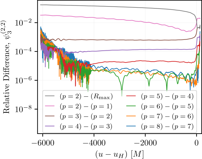
Figure 5: Relative difference of $\psi_{3}^{(2,2)}$ computed from successive extrapolation orders for a precessing binary black hole inspiral, merger, and ringdown. The extrapolation order $p=2$ waveform is compared with the unextrapolated waveform of the outermost extraction radius. The formation of the common horizon occurs at time $u_{H}$. The time-averaged value of each curve is the value of a point for the $\psi_{3}^{(2,2)}$ curve in Fig. 4.

IV.2.2 Bondi Gauge Analysis

The Bianchi identities provide a convenient tool to provide a self-consistency test on asymptotic NR waveforms. In an asymptotic spacetime, Bondi gauge is any choice of coordinates in which the metric and its derivatives approach Minkowski spacetime asymptotically. Our extrapolation procedure assumes an asymptotically flat spacetime, which should result in Bondi-gauge waveforms on $\mathscr{I}^{+}$. By taking the Bianchi identities written in the Newman-Penrose formalism and applying the assumptions for Bondi gauge, we are left with a set of constraint equations that must be satisfied for any consistent set of Bondi gauge waveforms,

$$\Psi_{4}^{0} =-\ddot{h}^{0},$$ (29a)

$$\Psi_{3}^{0} =\frac{1}{\sqrt{2}}\eth\dot{h}^{0},$$ (29b)

$$\dot{\Psi}_{3}^{0} =-\frac{1}{\sqrt{2}}\eth\Psi_{4}^{0},$$ (29c)

$$\dot{\Psi}_{2}^{0} =-\frac{1}{\sqrt{2}}\eth\Psi_{3}^{0}+\frac{1}{4}\bar{h}^{0}\Psi_{4}^{0},$$ (29d)

$$\dot{\Psi}_{1}^{0} =-\frac{1}{\sqrt{2}}\eth\Psi_{2}^{0}+\frac{1}{2}\bar{h}^{0}\Psi_{3}^{0},$$ (29e)

$$\dot{\Psi}_{0}^{0} =-\frac{1}{\sqrt{2}}\eth\Psi_{1}^{0}+\frac{3}{4}\bar{h}^{0}\Psi_{2}^{0}.$$ (29f)

where an overdot signifies a derivative with respect to $u$. We are using the $\eth$ operator as defined for a spin-weighted function $f$ of spin weight $s$,

$$\eth f=-\frac{\left(\sin\theta\right)^{s}}{\sqrt{2}}\left(\frac{\partial}{\partial\theta}+\frac{i}{\sin\theta}\frac{\partial}{\partial\phi}\right)\left[\left(\sin\theta\right)^{-s}f\right],$$ (30)

which acts on the spin-weighted spherical harmonics as the ladder-operator,

$$\eth\,{}_{s}Y_{\ell m} =\sqrt{\frac{1}{2}(\ell-s)(\ell+s+1)}\;{}_{s+1}Y_{\ell m},$$ (31a)

$$\bar{\eth}\,{}_{s}Y_{\ell m} =-\sqrt{\frac{1}{2}(\ell+s)(\ell-s+1)}\;{}_{s-1}Y_{\ell m}.$$ (31b)

The factors that appear in Eqs. (29) may seem to disagree with the existing literature. See Appendix B for a discussion on these differences. The derivation of Eqs. (29b–29f) assumes that tetrads have been chosen such that $h^{0}=\bar{\sigma}^{0}$; the Bianchi identities themselves do not depend directly on $h$. Following the considerations in Sec. II.3 and Appendix C, the use of $h$ in these equations leaves a possible subleading term of $\sigma$ unaccounted for. This would mean that these constraint equations with $h$ are only approximate constraints. Nonetheless, comparisons with CCE waveforms suggest that this subleading term in $\sigma$ is negligible for our current precision, and even these approximate constraints are satisfied to a tolerance that allows for practical application.

Using the information from Fig. 4 and plots like Fig. 5 for each asymptotic quantity, we chose the following values of $p$ for each waveform to test the Bondi gauge constraints:

• $p=7$ for $\psi_{4}$ and $\psi_{3}$

• $p=5$ for $\psi_{2}$ and $h^{0}$

• $p=3$ for $\psi_{1}$

• $p=2$ for $\psi_{0}$

Using these waveforms, we can find the relative magnitude of the violations of Eqs. (29). The deviation from equality is scaled with respect to the magnitude of the left-hand side of the equation. For each mode, we take the time average of the violation, setting the initial time to when the initial junk radiation has passed and setting the final time to $u_{H}+80\,M$. The results are plotted in Fig. 6. The time derivatives were performed by fitting a cubic spline to the waveform and then evaluating the derivative of the spline. Since the sampling of the data is not uniform in time—with a higher density of points near merger—we performed a minimization of the violations while varying the density of the time sampling used in each time derivative.

For the modes that predominantly contribute to the waveform—the $(\ell,\pm\ell)$ and $\left(\ell,\pm(\ell-1)\right)$ modes—we see violations from Bondi gauge between $\mathcal{O}(10^{-5})$ and $\mathcal{O}(10^{-2})$. The $h^{0}$ and $\psi_{4}$ waveforms are of the greatest interest for gravitational wave astronomy. Although we cannot make any direct statements on how well any individual waveform satisfies the Bondi constraints, we can parse out some more information by considering Eqs. (29a–29c). All three equations only involve $(h^{0},\psi_{4},\psi_{3})$, and Eq. (29c) is the only constraint equation that does not include $h^{0}$. Although Eq. (29b) and Eq. (29c) are effectively the same relation, just differing by an overall time derivative, the latter demonstrates smaller violations by roughly half an order of magnitude. This may imply that a large part of the violation is due to $h^{0}$, which would not be unreasonable given that an entirely different extraction procedure is used for the strain. It has also been observed in several SXS waveforms that the $h^{0}$ waveform seems to contain more noise than the $\psi_{4}$ waveform. A further analysis of the RWZ extraction procedure for the strain may shed more light on this.

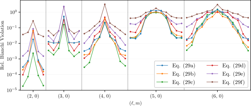
Figure 6: The relative magnitude of the violation of the Bianchi identity constraints, Eqs. (29), by numerical Bondi-gauge asymptotic waveforms of a binary black hole coalescence. For each value of $\ell$, the modes are plotted from $(\ell,-\ell)$ to $(\ell,\ell)$ in order of increasing $m$. Each letter in the legend refers to the equation in Eqs. (29) that is being plotted. Specifically, the values plotted here are the left-hand sides of the equations minus the right-hand sides, all scaled by magnitude of the left-hand sides. A full discussion of this data is found in Sec. IV.2.2 after Eqs. (31). The modes for each value of $\ell$ have been connected for ease of visualization.

V Conclusion

All gravitational waveforms have an inherent infinite-dimensional set of gauge freedoms. When working with asymptotic waveforms at $\mathscr{I}^{+}$, we can understand transformations between waveforms in different asymptotic coordinates via the BMS group. Before attempting to build any phenomenological or surrogate models from NR waveforms, we must both ensure that the waveforms are free from all near-field effects and also be able to systematically fix the BMS gauge freedom. This is crucial if we want to separate artifacts of gauge from the actual physical information in the waveform.

A method for fixing the BMS gauge freedom has been proposed by Moreschi [33, 34], which requires reliable extraction of the asymptotic quantities of $h$, $\Psi_{4}$, $\Psi_{3}$, and $\Psi_{2}$. The extraction procedure implemented in this paper, using the real characteristic fields of the Weyl tensor evolution equations, is efficient and readily implementable given the standard 3+1 variables from any NR code. We have demonstrated a successful implementation in the Spectral Einstein Code.

The extraction procedure achieves its efficiency at the cost of using a tetrad choice that is not guaranteed to be orthonormal nor aligned with the principal null directions of the spacetime. However, we have demonstrated that nonorthonormal and misaligned tetrads can still be used in getting the asymptotic Weyl scalars as long as the spurious effects of the tetrad choice fall off with radius at orders subleading to those specified by the peeling theorem. This paper has explored an extrapolation procedure by which we can determine the asymptotic waveform data from the finite-radius extracted data. Using a coordinate-shifted Kerr metric, we have shown that the extraction and extrapolation procedure is able to recover the correct asymptotic values. For a precessing, unequal mass ratio, binary black hole coalescence we have shown that we can find convergence in the extrapolation procedure for $h$, $\Psi_{4}$, $\Psi_{3}$, and $\Psi_{2}$, while extrapolation still leads to improvement for $\Psi_{1}$ and $\Psi_{0}$. We discussed several methods to reduce the effect of junk radiation in waveforms resulting from binary black hole initial data.

There are several limiting factors to the extrapolation procedure. As ansatzes, we have taken the choice of conformal scaling function Eq. (19), the expansion of the Weyl scalars as a polynomial Eq. (14), and the approximate parametrization of null rays Eq. (17). An improvement in any one of these may improve the extrapolation convergence. Despite these limitations, we are able to obtain numerical waveforms for the full set of Weyl scalars that agree with those of an asymptotic Bondi-gauge spacetime up to a relative error of $\mathcal{O}(10^{-2})$ for the first few dominant modes. For the waveforms specifically required for the BMS gauge-fixing procedure, we are able to obtain waveforms that agree with asymptotic Bondi-gauge waveforms up to a relative error of $\mathcal{O}(10^{-3})$. Further analysis can be performed once other extraction procedures, such as CCE, produce asymptotic waveforms to compare against.

By expanding upon the robust and well established wave extraction method of SpEC, we have presented the first production-level waveforms for the entire set of Weyl scalars that are immediately ready for use as tools for gravitational wave astronomy. Having the full set of Weyl scalars allows us to use the Bianchi identities to test our extracted waveforms against exact general relativity and provide hard upper bounds on their accuracy. This analysis is straightforward to perform and can test each waveform mode individually, as we have demonstrated in Fig. 6. A small public catalog of simulations with the full set of Weyl scalar waveforms will soon be made available. The Weyl characteristic field extraction-extrapolation procedure that we have presented has now set the stage for a reliable method that will finally provide the gravitational wave astronomy community with completely gauge-fixed waveforms.

VI Acknowledgments

We are grateful to Will Throwe, Eamonn O’Shea, Cristóbal Armaza, and Gabriel Bonilla for insightful discussions. Computations were performed with the High Performance Computing Center and the Wheeler cluster at Caltech. This work was supported in part by the Sherman Fairchild Foundation and by NSF Grants No. PHY-2011961, No. PHY-2011968, and No. OAC-1931266 at Caltech and NSF Grants No. PHY-1912081 and No. OAC-1931280 at Cornell.

Appendix A Complex Weyl Characteristic Fields

Requiring the Faraday tensor to be divergenceless and satisfy the Bianchi identity results in two constraint equations and two evolution equations for the Maxwell electric and magnetic fields. In a similar way, requiring the Weyl tensor to be divergenceless and satisfy the Bianchi identities,

$$\nabla_{[a}C_{bc]de} =0,$$ (32a)

$$\nabla^{a}C_{abcd} =0,$$ (32b)

results in two constraint equations and two evolution equations for $E_{ij}$ and $B_{ij}$. Since we are interested in the propagation of radiation, we will focus on the evolution equations. Just as in the Maxwell case, we have two coupled evolution equations for $E_{ij}$ and $B_{ij}$, which we can combine into a single equation,

$$\partial_{t}Q_{ij}-N^{k}\partial_{k}Q_{ij}-iN^{k}\partial_{k}Q_{l(i}\epsilon_{j)}{}^{kl}=S_{Q},$$ (33)

where $Q_{ij}=E_{ij}+iB_{ij}$, and $S_{Q}$ is all of the source terms. These source terms are purely algebraic in $E_{ij}$ and $B_{ij}$. We can further decompose the quantity $Q_{ij}$ with respect to the geometry of the simulation domain. In the region we would be extracting $Q_{ij}$, the domain is constructed of concentric spherical shells, that is, a radial foliation of the spatial hypersurfaces. If we have a 2-sphere metric $q_{ij}$ and an outgoing spatial radial vector $r^{a}$, then the spatial and symmetric tensor $Q_{ij}$ can be decomposed irreducibly into a scalar function $\mathcal{C}$, a vector $\mathcal{C}_{i}$, and a transverse-traceless tensor $\mathcal{C}_{ij}$,

$$Q_{ij} =\mathcal{C}\left(r_{i}r_{j}-\frac{1}{2}q_{ij}\right)+2r_{(i}\mathcal{C}_{j)}+\mathcal{C}_{ij},$$ (34a)

$$\mathcal{C} =\left(E_{ij}+iB_{ij}\right)r^{i}r^{j},$$ (34b)

$$\mathcal{C}_{i} =\left(E_{jk}+iB_{jk}\right)r^{j}q^{k}{}_{i},$$ (34c)

$$\mathcal{C}_{ij} =\left(E_{kl}+iB_{kl}\right)\left(q^{k}{}_{i}q^{l}{}_{j}+\frac{1}{2}q^{kl}q_{ij}\right).$$ (34d)

Thus we can express the Weyl scalars in terms of the complex characteristic fields,

$$\Psi_{4} =\mathcal{C}_{ij}\bar{m}^{i}\bar{m}^{j},$$ (35a)

$$\Psi_{3} =\frac{1}{\sqrt{2}}\mathcal{C}_{i}\bar{m}^{i},$$ (35b)

$$\Psi_{2} =\frac{1}{2}\mathcal{C},$$ (35c)

$$\Psi_{1} =-\frac{1}{\sqrt{2}}\mathcal{C}_{i}m^{i},$$ (35d)

$$\Psi_{0} =\mathcal{C}_{ij}m^{i}m^{j}.$$ (35e)

It is simpler numerically to store and work with real numbers. Using the following identities [42],

$$im_{i} =-r^{j}m^{k}\epsilon_{ijk},$$ (36a)

$$i\bar{m}_{i} =r^{j}\bar{m}^{k}\epsilon_{ijk},$$ (36b)

we can rewrite the three complex fields as the six real characteristic fields in Eqs. 6.

Appendix B Tetrad Conventions

The goal of this section is to express the relations between asymptotic quantities in Bondi gauge in a way that is completely agnostic of sign convention and scale factors. As such, all the assumptions and results in this section are only valid with a Minkowski metric. We start by defining a sign variable $s_{0}$ to account for different choices of the metric signature,

$$s_{0}=\begin{cases}1&\text{for metric signature }(-,+,+,+)\\ -1&\text{for metric signature }(+,-,-,-)\end{cases}$$ (37)

For the sake of simplicity, all variables introduced in this section that are named $s_{\text{n}}$ will be used to generalize a sign convention and can only take the value $\pm 1$. In this section, $g_{ab}$ and $\eta_{ab}$ are the $(-,+,+,+)$ signature metrics and explicit factors of $s_{0}$ will be used to account for metric signature.

In the literature, it is common to define a complex null tetrad by first constructing $l_{a}$ to be a null vector tangent to outgoing null hypersurfaces parametrized by constant retarded time $u$,

$$l_{a}\propto(du)_{a}.$$ (38)

The ingoing null tetrad vector $n^{a}$ is then defined by enforcing the normalization $l_{a}n^{a}=-s_{0}$. There remains the freedom to introduce a scaling by $\lambda$ that still satisfies the normalization, $(\lambda l_{a})(\lambda^{-1}n^{a})=-s_{0}$. We can absorb this freedom, which includes a sign ambiguity, into the definition of $l_{a}$ by defining it as

$$l_{a}=-\frac{\lambda}{\sqrt{2}}(dt-dr)_{a}.$$ (39)

While $\lambda$ parametrizes the boost freedom of the tetrad, there is still a spin freedom on the choice of $m^{a}$, for which we can see that $m^{a}\mapsto e^{i\Theta}m^{a}$ does not affect the normalization $m^{a}\bar{m}_{a}=s_{0}$. Therefore, we absorb this freedom, parametrized by $0\leq\Theta<2\pi$, into the definition of $m^{a}$,

$$m_{a}=\frac{e^{i\Theta}}{\sqrt{2}}\left(d\theta+id\phi\right)_{a},$$ (40)

This orientation is chosen so that for $\Theta=0$, on the $z$ axis we would find that $(d\theta)_{a}$ points along the positive $x$ axis. Throughout this section we are defining $\eth$ as appropriate to each author’s definition of $m^{a}$.

The Christoffel symbols of the second kind contain no factors of $s_{0}$ so they are agnostic to metric signature,

$$\Gamma^{c}_{ab}=\frac{1}{2}g^{cd}\left(\partial_{b}g_{da}+\partial_{a}g_{db}-\partial_{d}g_{ab}\right),$$ (41)

Using the above definition for the Christoffel symbol, there is a choice of sign convention on the definition of Riemann tensor, which we parametrize by $s_{3}$,

$$s_{3}R^{a}{}_{bcd}=\partial_{c}\Gamma^{a}_{db}-\partial_{d}\Gamma^{a}_{cb}+\Gamma^{a}_{ce}\Gamma^{e}_{db}-\Gamma^{a}_{de}\Gamma^{e}_{cb},$$ (42)

Note that a factor of $s_{0}$ appears for the lowered-index Riemann tensor,

$$R_{abcd}=s_{3}s_{0}\left(\partial_{c}\Gamma_{adb}-\partial_{d}\Gamma_{acb}+\Gamma_{ace}\Gamma^{e}_{db}-\Gamma_{ade}\Gamma^{e}_{cb}\right).$$ (43)

We then need to define the sign variables $s_{1}$ and $s_{2}$ to take in account the choice of sign in the definitions of the Weyl scalars and the Newman-Penrose shear $\sigma$,

$$\Psi_{4} =s_{1}C_{abcd}n^{a}\bar{m}^{b}n^{c}\bar{m}^{d},$$ (44a)

$$\sigma =s_{2}m^{a}m^{b}\nabla_{a}l_{b},$$ (44b)

where here the terms on the right-hand sides are in each author’s own convention. The Bondi gauge Bianchi identities can now be written as

$$\dot{\Psi}_{3}^{0} =-\frac{\lambda e^{i\Theta}}{\sqrt{2}}\eth\Psi_{4}^{0},$$ (45a)

$$\dot{\Psi}_{2}^{0} =-\frac{\lambda e^{i\Theta}}{\sqrt{2}}\eth\Psi_{3}^{0}+\frac{1}{\sqrt{2}}s_{0}s_{2}\lambda\sigma^{0}\Psi_{4}^{0},$$ (45b)

$$\dot{\Psi}_{1}^{0} =-\frac{\lambda e^{i\Theta}}{\sqrt{2}}\eth\Psi_{2}^{0}+\frac{2}{\sqrt{2}}s_{0}s_{2}\lambda\sigma^{0}\Psi_{3}^{0},$$ (45c)

$$\dot{\Psi}_{0}^{0} =-\frac{\lambda e^{i\Theta}}{\sqrt{2}}\eth\Psi_{1}^{0}+\frac{3}{\sqrt{2}}s_{0}s_{2}\lambda\sigma^{0}\Psi_{2}^{0}.$$ (45d)

A list of the conventions for various papers is given in Table 1.

We can also define a parameter $\zeta$ to account for different scaling factors of the gravitational-wave strain,

$$h=\zeta^{-1}\left[\frac{1}{2}\left(h_{\theta\theta}-h_{\phi\phi}\right)-ih_{\theta\phi}\right],$$ (46)

where $h_{ab}=s_{0}(g_{ab}-\eta_{ab})$. From this we can write the relation between $\Psi_{4}^{0}$ and $h^{0}$ as

$$\Psi_{4}^{0} =-\left(s_{1}s_{3}\zeta\lambda^{-2}e^{-2i\Theta}\right)\ddot{h}^{0},$$ (47)

In order to convert a quantity in the SpEC convention to a different convention, the appropriate factors can be determined by

$$\Psi^{0\,[\text{X}]}_{n} =s_{0}s_{1}s_{3}\left(\lambda e^{i\Theta}\right)^{2-n}\Psi^{0\,[\text{SpEC}]}_{n},$$ (48a)

$$h^{0\,[\text{X}]} =s_{0}\zeta^{-1}e^{-2i\Theta}h^{0\,[\text{SpEC}]},$$ (48b)

where all of the parameters are from the column of convention [X] in the table. Although we can easily relate $h^{0}$ and $\Psi_{4}^{0}$ between different conventions, the situation is far more complicated for $\sigma^{0}$. These complexities will be discussed in Appendix C.

	SpEC	MB	NP	ADLK	BR	C
$s_{0}$	$1$	$-1$	$-1$	$1$	$1$	$-1$
$s_{1}$	$1$	$1$	$-1$	$1$	$-1$	$-1$
$s_{2}$	$1$	$1$	$1$	$-1$	N/A	$1$
$s_{3}$	$1$	$1$	$1$	$1$	$1$	$1$
$\lambda$	$1$	$-\sqrt{2}$	$-\sqrt{2}$	$-\sqrt{2}$	$1$	$-\sqrt{2}$
$\Theta$	$0$	$0$	$\pi$	$0$	$0$	$0$
$\zeta$	$1$	$2$	N/A	$1$	$1$	N/A
reference	[25]	[2, 5]	[58]	[59]	[30]	[60]

Table 1: Sign conventions and scaling factors for various papers. For convenience, a shorthand name for each convention is given in the first row. N/A signifies that the particular convention is not specified in that paper.

Appendix C Subleading tetrad hazards

In Sec. II.3, we discussed that in the asymptotic limit the Weyl scalars and the strain $h$ are invariant under tetrad transformations that leave the leading order tetrad behavior unchanged. However, this does not hold for all the Newman-Penrose scalars. Most importantly it does not hold for the shear $\sigma$. Although we are not extracting $\sigma$ from simulations, the analysis of numerical waveforms using the BMS group still requires understanding how $\sigma$ relates to the Weyl scalars and $h$. Furthermore, a formidable difficulty arises when attempting to establish a connection with the literature. Waveform quantities cannot be generally converted between the different formalisms because the subleading tetrad behavior is often not specified sufficiently. This appendix will explore the effects of subleading tetrad behavior on the asymptotic quantities that are of primary interest to the study of gravitational radiation.

The waveform quantities that fall off as $1/r^{2}$ or faster are vulnerable to dependence on the definitions of the tetrads off $\mathscr{I}^{+}$. The reason for these corrections is simple, but calculating them is laborious and establishing complete agreement of the competing conventions is deeply vexing, especially because the subleading behavior in $1/r$ of tetrads is not nearly so universally prescribed as the leading behavior described in Appendix B.

The discussion of this appendix is closely related to the concept of tetrad rotations, which is covered at length in previous publications [61, 62]. The challenge that we face here, however, distinguishes itself because the distinct calculations, especially those performed during Cauchy evolution, often do not guarantee that the tetrad basis is orthonormal or null in the bulk of the spacetime, only at its boundary. Therefore, the alteration between conventions is somewhat more free even than generic $\mathcal{O}(1/r)$ tetrad rotations.

To motivate this discussion, first consider the havoc generated by the simple alteration of the angular tetrads at subleading order in $1/r$ (holding for this illustrative sketch $l^{\prime}=l$ and $n^{\prime}=n$),

$$m^{\prime\alpha}=m^{\alpha}+\frac{1}{r}\left(Am^{\alpha}+B\bar{m}^{\alpha}\right).$$ (49)

In particular, the Newman-Penrose spin coefficient $\sigma=m^{\alpha}m^{\beta}\nabla_{\alpha}l_{\beta}\sim\mathcal{O}(r^{-2})$ is altered as

$$\sigma^{\prime}=\sigma+\frac{1}{r}\left(2B\rho+2A\sigma\right)+\frac{1}{r^{2}}\left(A^{2}\sigma+2AB\rho+B^{2}\bar{\sigma}\right),$$ (50)

where $\rho=\bar{m}^{\alpha}m^{\beta}\nabla_{\alpha}l_{\beta}$, and $\rho=\bar{\rho}$ by assumption. However, because $\rho\sim\mathcal{O}(1/r)$, we find that the definition of $\sigma$ that we had hoped to standardize now depends on the subleading values of the tetrad $m^{\alpha}$. Fortunately, in this restricted case, none of the leading contributions to the Weyl scalars are altered, but it is not hard to construct alterations to $l$ and $n$ at subleading order in $1/r$ that would cause disruption all down the chain of Weyl scalars according to the peeling theorem.

In Appendix Sec. C.1, we derive the alteration between the SpEC tetrad and the tetrad used in SXS CCE [63]. In Appendix Sec. C.2 we expand the correction between the SXS CCE tetrad and a generic asymptotic null tetrad, which is an easier comparison to perform because we can take advantage of the properties of null tetrad rotations. In each case, we propagate the tetrad alteration to determine the final modifications to the asymptotic values of the waveform quantities $h,\sigma,\Psi_{4},\Psi_{3},\Psi_{2},\Psi_{1}$, and $\Psi_{0}$.

In each of these sections, we denote the tetrads of the various conventions with text subscripts or superscripts (e.g. $l_{\text{SpEC}}$ for the SpEC tetrad convention). To determine the subleading dependence of the tetrads in the different conventions, it is often necessary to expand the tetrads in powers of inverse $r$, which we denote with the order of inverse $r$ in parentheses (e.g. $l_{\text{CCE}}^{(0)}$). Implicitly, this is written as the $r$ coordinate in the SpEC convention, but because we only work in a limited expansion in powers of inverse $r$, all of the statements would be unchanged if working in the Bondi-Sachs $\mathring{r}$. To avoid confusion, we do not use the superscript $0$ as in the body of the text to denote the leading contribution to a waveform quantity asymptotically. Instead, we use the explicit power of $r$ explicitly, writing for instance $\Psi_{4}^{0}$ as $\Psi_{4}^{(1)}$.

C.1 Subleading tetrads in CCE

In this section, we use the tetrads for a CCE formalism described in [63],

$$m^{\mu}_{\text{CCE}} =-\frac{1}{\sqrt{2}r}\left(\sqrt{\frac{K+1}{2}}q^{\mu}-\sqrt{\frac{1}{2(1+K)}J}\bar{q}^{\mu}\right),$$ (51a)

$$n^{\mu}_{\text{CCE}} =\sqrt{2}e^{-2\beta}\bigg{(}\delta^{\mu}{}_{u}-\frac{1}{2}\left(1+rW\right)\delta^{\mu}{}_{r}$$

$$\hskip 54.06006pt+\frac{1}{2}\bar{U}q^{\mu}+\frac{1}{2}U\bar{q}^{\mu}\bigg{)},$$ (51b)

$$l^{\mu}_{\text{CCE}} =\frac{1}{\sqrt{2}}\delta^{\mu}{}_{r},$$ (51c)

where the Bondi-Sachs scalars $J,K,\beta,V,U$ and coordinates are as defined in [63], which each represent components of the metric in Bondi-Sachs coordinates. We assume that the tetrads constructed in Eq. (12) for the SpEC Cauchy simulation are in agreement with the CCE tetrad, Eqs. (51), asymptotically. We expand the relation in powers of inverse $r$, denoting (dropping the “CCE” for brevity, understanding that the order subscripts in this appendix section will apply exclusively to the tetrad derived in the CCE formalism),

$$m^{\mu}_{\text{CCE}} =m^{\mu}_{(0)}+\frac{1}{r}m^{\mu}_{(1)}+\mathcal{O}(r^{-2}),$$ (52a)

$$l^{\mu}_{\text{CCE}} =l^{\mu}_{(0)}+\frac{1}{r}l^{\mu}_{(1)}+\mathcal{O}(r^{-2}),$$ (52b)

$$n^{\mu}_{\text{CCE}} =n^{\mu}_{(0)}+\frac{1}{r}n^{\mu}_{(1)}+\mathcal{O}(r^{-2}).$$ (52c)

Importantly, when attempting to compare the tetrads in the disparate coordinate systems, we need to be aware of the alterations associated with the conversion between the Bondi-Sachs coordinate system and the Cauchy coordinates. For simplicity of the current presentation, we expand the Bondi-Sachs coordinates in terms of the Cauchy radial coordinate,

$$\mathring{u} =u+\frac{1}{r}\mathring{u}^{(1)}+\mathcal{O}(r^{-2}),$$ (53a)

$$\mathring{r} =r+\mathring{r}^{(0)}+\frac{1}{r}\mathring{r}^{(1)}+\mathcal{O}(r^{-2}),$$ (53b)

$$\mathring{x}^{A} =x^{A}+\frac{1}{r}\mathring{x}^{(1)A}+\mathcal{O}(r^{-2}),$$ (53c)

Unfortunately, the differences between these coordinate systems depend on the myriad choices in constructing a CCE evolution associated with a particular Cauchy evolution, including extraction surface and data on the initial hypersurface. The quantities $\mathring{u}^{(1)}$, $\mathring{r}^{(1)}$, and $\mathring{x}^{(1)A}$ can be determined numerically for a particular Cauchy and CCE evolution, but practical implementations of that calculation is beyond the scope of the current discussion.

A contribution $r^{(0)}$ to Eq. (53b), should it be nonvanishing, has even more dire consequences on attempts to establish asymptotic correspondence. This coordinate alteration impacts the leading tetrads,

$$m_{(0)}^{\mu}=m^{\mu}_{\text{SpEC}}+l^{\mu}m^{\nu}_{\text{SpEC}}\partial_{\nu}\mathring{r}^{(0)},$$ (54a)

$$n_{(0)}^{\mu}=n^{\mu}_{\text{SpEC}}+l^{\mu}n^{\nu}_{\text{SpEC}}\partial_{\nu}\mathring{r}^{(0)}.$$ (54b)

Fortunately, such impact is easy to notice, as it will manifest as a nonvanishing inner product $n^{\mu}_{\text{SpEC}}g_{\mu\nu}n^{\nu}_{\text{SpEC}}$ or $n^{\mu}_{\text{SpEC}}g_{\mu\nu}m^{\nu}_{\text{SpEC}}$ at $\mathscr{I}^{+}$. We will assume from here on in this appendix that any such pathology has been avoided in the Cauchy code and that we may safely set $\mathring{r}^{(0)}=0$. Therefore, the leading tetrads at $\mathscr{I}^{+}$ are assumed to be in agreement between the Cauchy code and CCE: $l^{\mu}_{(0)}=l^{\mu}_{\text{SpEC}}$, $m^{\mu}_{(0)}=m^{\mu}_{\text{SpEC}}$, $n^{\mu}_{(0)}=n^{\mu}_{\text{SpEC}}$.

Given the agreement between asymptotic tetrads, we can use the subleading metric contracted with the leading tetrads (from either formalism) to infer the metric components that act as inputs to the tetrad definitions in Eqs. (51). In particular,

$$J^{(1)} =g_{mm}^{(1)},$$ (55a)

$$U^{(2)} =g_{nm}^{(1)},$$ (55b)

$$\beta^{(1)} =\frac{1}{2}g_{nl}^{(1)},$$ (55c)

$$W^{(2)} =-\frac{1}{2}g_{nn}^{(1)}.$$ (55d)

When all effects are taken into account, the subleading tetrad expressions for the CCE formalism are

$$m_{(1)}^{\mu} =-J^{(1)}\bar{m}^{\mu}_{(0)},$$ (56a)

$$n_{(1)}^{\mu} =\sqrt{2}\partial_{u}\mathring{u}^{(1)}(n_{(0)}^{\mu}+l_{(0)}^{\mu})+\sqrt{2}\partial_{u}\mathring{r}^{(1)}l^{\mu}_{(0)}$$

$$\hskip 8.53581pt+\frac{1}{\sqrt{2}}\partial_{u}\mathring{x}^{(1)A}\left(m^{(0)}_{A}\bar{m}_{(0)}^{\mu}+\bar{m}^{(0)}_{A}m_{(0)}^{\mu}\right)$$

$$\hskip 8.53581pt-2\sqrt{2}\beta^{(1)}n^{\mu}_{(0)}-W^{(2)}l^{\mu}_{(0)}$$

$$\hskip 8.53581pt-\bar{U}^{(2)}m_{(0)}^{\mu}-U^{(2)}\bar{m}_{(0)}^{\mu},$$ (56b)

$$\equiv n^{(1)}_{n}l^{\mu}_{(0)}+n^{(1)}_{l}n^{\mu}_{(0)}+n^{(1)}_{m}\bar{m}^{\mu}_{(0)}+n^{(1)}_{\bar{m}}m^{\mu}_{(0)},$$ (56c)

$$l_{(1)}^{\mu} =0.$$ (56d)

To summarize, the subleading contributions to the $m$ tetrad vector amounts simply to a $\mathcal{O}(r^{-1})$ rotation in the $m$, $\bar{m}$ plane, the $n$ tetrad vector has contributions along all of the original tetrad directions, and the subleading $l$ tetrad vector vanishes. We emphasize that the tetrad corrections between the CCE and SpEC tetrads are not simply a tetrad rotation, so we must consider carefully the effects on the waveform quantities.

Given the above CCE tetrad, Eqs. (51), with explicit $\mathcal{O}(r^{-1})$ parts, Eqs. (56), the conversion between the waveform quantities derived from the SpEC tetrad and CCE tetrad are as follows,

$$h^{(1)\text{CCE}} =h^{(1)\text{SpEC}},$$ (57a)

$$\sigma^{(2)\text{CCE}} =\sigma^{(2)\text{SpEC}}$$

$$\hskip 14.22636pt-J^{(1)}\left(\rho^{(1)\text{SpEC}}+\bar{\rho}^{(1)\text{SpEC}}\right),$$ (57b)

$$\Psi_{4}^{(1)\text{CCE}} =\Psi_{4}^{(1)\text{SpEC}},$$ (57c)

$$\Psi_{3}^{(2)\text{CCE}} =\Psi_{3}^{(2)\text{SpEC}},$$ (57d)

$$\Psi_{2}^{(3)\text{CCE}} =\Psi_{2}^{(3)\text{SpEC}},$$ (57e)

$$\Psi_{1}^{(4)\text{CCE}} =\Psi_{1}^{(4)\text{SpEC}},$$ (57f)

$$\Psi_{0}^{(5)\text{CCE}} =\Psi_{0}^{(5)\text{SpEC}}.$$ (57g)

The main take-away from this calculation is that the leading strain and all of the Weyl scalars agree between the two formalisms. The shear, however, is a bit of a sticking point. In particular, if the $\rho$ mimics typical Kerr behavior asymptotically and $\sigma^{\text{SpEC}}$ is asymptotically equal to the leading part of the strain, the $\sigma^{\text{CCE}}$ will differ from $\sigma^{\text{SpEC}}$ by an overall sign change.

C.2 Tetrad rotations between CCE and other formulations

Many of the methods of choosing a Newman-Penrose construction at $\mathscr{I}^{+}$ do not completely specify the tetrad behavior at subleading order. In this section, we will make some fairly general assumptions about the construction of the subleading tetrad contribution, and derive the corrections between possible choices in those constructions.

First, let us consider the case of unrestricted null tetrad rotations. The condition that the tetrads remain orthonormal and null constrains the set of degrees of freedom,

$$\bar{m}^{\mu}_{\text{G}} =\bar{m}^{\mu}_{\text{CCE}}+\frac{1}{r}\bigg{(}-\bar{m}^{\text{G}(1)}_{l}n^{\mu}_{\text{CCE}}-\bar{m}^{\text{(}1)G}_{n}l^{\mu}_{\text{CCE}}$$

$$\hskip 68.28644pt+\bar{m}^{\text{(}1)G}_{m}\bar{m}^{\mu}_{\text{CCE}}\bigg{)}+\mathcal{O}(r^{-2}),$$ (58a)

$$m^{\mu}_{\text{G}} =m^{\mu}_{\text{CCE}}+\frac{1}{r}\bigg{(}-m^{\text{G}(1)}_{l}n^{\mu}_{\text{CCE}}-m^{\text{(}1)G}_{n}l^{\mu}_{\text{CCE}}$$

$$\hskip 68.28644pt+\bar{m}^{\text{(}1)G}_{m}m^{\mu}_{\text{CCE}}\bigg{)}+\mathcal{O}(r^{-2}),$$ (58b)

$$n^{\mu}_{\text{G}} =n^{\mu}_{\text{CCE}}+\frac{1}{r}\bigg{(}-n^{\text{G}(1)}_{l}n^{\mu}_{\text{CCE}}-\bar{m}^{\text{(}1)G}_{n}m^{\mu}_{\text{CCE}}$$

$$\hskip 68.28644pt-m^{\text{G}(1)}_{n}\bar{m}^{\mu}_{\text{CCE}}\bigg{)}+\mathcal{O}(r^{-2}),$$ (58c)

$$l^{\mu}_{\text{G}} =l^{\mu}_{\text{CCE}}+\frac{1}{r}\bigg{(}n^{\text{G}(1)}_{l}l^{\mu}_{\text{CCE}}-\bar{m}^{\text{(}1)G}_{l}m^{\mu}_{\text{CCE}}$$

$$\hskip 68.28644pt-m^{\text{G}(1)}_{l}\bar{m}^{\mu}_{\text{CCE}}\bigg{)}+\mathcal{O}(r^{-2}).$$ (58d)

Generic rotations of the form Eq. (58) give rise to numerous corrections to the waveform quantities,

$$h^{(1)\text{G}}=h^{(1)\text{CCE}},$$ (59a)

$$\Psi_{4}^{(1)\text{G}}=\Psi_{4}^{(1)\text{CCE}},$$ (59b)

$$\Psi_{3}^{(2)\text{G}}=\Psi_{3}^{(2)\text{CCE}}-\Psi_{4}^{(1)\text{CCE}}m^{\text{(}1)G}_{l},$$ (59c)

$$\Psi_{2}^{(3)\text{G}}=$$

$$\hskip 14.22636pt\Psi_{2}^{(3)\text{CCE}}-4\Psi_{3}^{(2)\text{CCE}}m^{\text{(}1)G}_{l}+2\Psi_{4}^{(1)\text{CCE}}\left(m_{l}^{\text{(}1)G}\right)^{2},$$ (59d)

$$\Psi_{1}^{(4)\text{G}}=$$

$$\hskip 14.22636pt\Psi_{1}^{(4)\text{CCE}}-2\Psi_{2}^{(3)\text{CCE}}m^{\text{(}1)G}_{l}+\bar{\Psi}_{3}^{(2)\text{CCE}}\bar{m}^{\text{(}1)G}_{l}m^{\text{(}1)G}_{l}$$

$$\hskip 14.22636pt-\bar{\Psi}_{4}^{(1)\text{CCE}}\left(\bar{m}^{\text{(}1)G}_{l}\right)^{2}m^{\text{(}1)G}_{l}+3\Psi_{3}^{(2)\text{CCE}}\left(m^{\text{(}1)G}_{l}\right)^{2}$$

$$\hskip 14.22636pt-\Psi_{4}^{(1)\text{CCE}}\left(m^{\text{(}1)G}_{l}\right)^{3},$$ (59e)

$$\Psi_{0}^{(5)\text{G}}=$$

$$\hskip 14.22636pt\Psi_{0}^{(5)\text{CCE}}-4\Psi_{1}^{(4)\text{CCE}}m^{\text{(}1)G}_{l}+5\Psi_{2}^{(3)}\left(m^{\text{(}1)G}_{l}\right)^{2}$$

$$\hskip 14.22636pt+\bar{\Psi}_{4}^{(1)\text{CCE}}\left(\bar{m}_{l}^{\text{(}1)G}\right)^{2}\left(m_{l}^{\text{(}1)G}\right)^{2}$$

$$\hskip 14.22636pt-4\Psi_{3}^{(2)\text{CCE}}\left(m_{l}^{\text{(}1)G}\right)^{2}+\Psi_{4}^{(1)}\left(m_{l}^{\text{(}1)G}\right)^{4},$$ (59f)

$$\sigma^{(2)\text{G}}=$$

$$\hskip 14.22636pt\sigma^{(2)\text{CCE}}-2\beta^{(1)}m^{\text{(}1)G}_{l}-\kappa^{(1)}m^{\text{(}1)G}_{n}-\tau^{(1)}m^{\text{(}1)G}_{l}$$

$$\hskip 14.22636pt+m_{\text{G}}^{(0)\mu}\nabla_{\mu}m^{\text{(}1)G}_{l}-m^{\text{(}1)G}_{l}n_{\text{G}}^{(0)\mu}\nabla_{\mu}m^{\text{(}1)G}_{l}.$$ (59g)

In Eqs. (59), we use the standard Newman-Penrose spin coefficient notation $\beta=1/2(n^{\alpha}m^{\beta}\nabla_{\beta}l_{\alpha}-\bar{m}^{\alpha}m^{\beta}\nabla_{\beta}m_{\alpha})$, $\kappa=-m^{\alpha}l^{\beta}\nabla_{\beta}l_{\alpha}$, and $\tau=-m^{\alpha}n^{\beta}\nabla_{\beta}l_{\alpha}$. This causes significant difficulty in comparing the results from different formalisms. However, there is a clear pattern associated with which parts of the tetrad rotation are important for the waveform comparisons.

In particular, if we merely impose that the null tetrad of the formulation we are comparing with the CCE results shares an $l$ tetrad vector, we find that the comparison expressions, Eqs. (59), simplifies greatly (denoting as LPG an “$l$-preserving generic” formalism that preserves the CCE $l$ vector – i.e. $l^{\mu}_{\text{CCE}}=l^{\mu}_{\text{LPG}}$),

$$h^{(1)\text{LPG}} =h^{(1)\text{CCE}},$$ (60a)

$$\sigma^{(2)\text{LPG}} =\sigma^{(2)\text{CCE}}-\kappa^{(1)}m^{\text{LPG}(1)}_{n},$$ (60b)

$$\Psi_{4}^{(1)\text{LPG}} =\Psi_{4}^{(1)\text{CCE}},$$ (60c)

$$\Psi_{3}^{(2)\text{LPG}} =\Psi_{3}^{(2)\text{CCE}},$$ (60d)

$$\Psi_{2}^{(3)\text{LPG}} =\Psi_{2}^{(3)\text{CCE}},$$ (60e)

$$\Psi_{1}^{(4)\text{LPG}} =\Psi_{1}^{(4)\text{CCE}},$$ (60f)

$$\Psi_{0}^{(5)\text{LPG}} =\Psi_{0}^{(5)\text{CCE}}.$$ (60g)

We emphasize that in the case where the $l$ tetrad vector is preserved between formalisms, all of the waveform quantities can be directly compared except for the shear $\sigma$. In particular, the relationship between the shear and the strain can differ between formalisms with different subleading tetrads, even if the tetrads evaluated at $\mathscr{I}^{+}$ are identical.

References

- Pürrer and Haster [2020] M. Pürrer and C.-J. Haster, Phys. Rev. Research 2, 023151 (2020), arXiv:1912.10055 [gr-qc] .
- Boyle [2016] M. Boyle, Phys. Rev. D 93, 084031 (2016), arXiv:1509.00862 [gr-qc] .
- Woodford et al. [2019] C. J. Woodford, M. Boyle, and H. P. Pfeiffer, Phys. Rev. D 100, 124010 (2019), arXiv:1904.04842 [gr-qc] .
- Kelly and Baker [2013] B. J. Kelly and J. G. Baker, Phys. Rev. D 87, 084004 (2013), arXiv:1212.5553 [gr-qc] .
- Lehner and Moreschi [2007] L. Lehner and O. M. Moreschi, Phys. Rev. D 76, 124040 (2007), arXiv:0706.1319 [gr-qc] .
- Khan et al. [2019] S. Khan, K. Chatziioannou, M. Hannam, and F. Ohme, Phys. Rev. D 100, 024059 (2019), arXiv:1809.10113 [gr-qc] .
- Field et al. [2014] S. E. Field, C. R. Galley, J. S. Hesthaven, J. Kaye, and M. Tiglio, Phys. Rev. X 4, 031006 (2014), arXiv:1308.3565 [gr-qc] .
- Bondi et al. [1962] H. Bondi, M. van der Burg, and A. Metzner, Proc. R. Soc. A 269, 21 (1962).
- Sachs [1962a] R. Sachs, Proc. R. Soc. A 270, 103 (1962a).
- Sachs [1962b] R. Sachs, Phys. Rev. 128, 2851 (1962b).
- Gualtieri et al. [2008] L. Gualtieri, E. Berti, V. Cardoso, and U. Sperhake, Phys. Rev. D 78, 044024 (2008), arXiv:0805.1017 [gr-qc] .
- Moreschi [1986] O. M. Moreschi, Classical Quantum Gravity 3, 503 (1986).
- Newman and Penrose [1962] E. Newman and R. Penrose, J. Math. Phys. 3, 566 (1962).
- Hinder et al. [2011] I. Hinder, B. Wardell, and E. Bentivegna, Phys. Rev. D 84, 024036 (2011), arXiv:1105.0781 [qr-qc] .
- Campanelli et al. [2006] M. Campanelli, B. J. Kelly, and C. O. Lousto, Phys. Rev. D 73, 064005 (2006), arXiv:gr-qc/0510122 .
- Gunnarsen et al. [1995] L. Gunnarsen, H. A. Shinkai, and K. I. Maeda, Classical Quantum Gravity 12, 133 (1995), arXiv:gr-qc/9406003 .
- López and Quiroga [2017] L. A. G. López and G. D. Quiroga, Rev. Mex. Fis. 63, 275 (2017), arXiv:1711.11381 [gr-qc] .
- Beetle et al. [2005] C. Beetle, M. Bruni, L. M. Burko, and A. Nerozzi, Phys. Rev. D 72, 024013 (2005), arXiv:0407012 [gr-qc] .
- Nerozzi et al. [2005] A. Nerozzi, C. Beetle, M. Bruni, L. M. Burko, and D. Pollney, Phys. Rev. D 72, 024014 (2005), arXiv:gr-qc/0407013v2 .
- Owen [2010] R. Owen, Phys. Rev. D 81, 124042 (2010), arXiv:1004.3768 [gr-qc] .
- Nichols et al. [2011] D. A. Nichols, R. Owen, F. Zhang, A. Zimmerman, J. Brink, Y. Chen, J. D. Kaplan, G. Lovelace, K. D. Matthews, M. A. Scheel, and K. S. Thorne, Phys. Rev. D 84, 124014 (2011), arXiv:1108.5486 [gr-qc] .
- Zhang et al. [2012a] F. Zhang, A. Zimmerman, D. A. Nichols, Y. Chen, G. Lovelace, K. D. Matthews, R. Owen, and K. S. Thorne, Phys. Rev. D 86, 084049 (2012a), arXiv:1208.3034 [gr-qc] .
- Nichols et al. [2012] D. A. Nichols, A. Zimmerman, Y. Chen, G. Lovelace, K. D. Matthews, R. Owen, F. Zhang, and K. S. Thorne, Phys. Rev. D 86, 104028 (2012), arXiv:1208.3038 [gr-qc] .
- Zhang et al. [2012b] F. Zhang, J. Brink, B. Szilágyi, and G. Lovelace, Phys. Rev. D 86, 084020 (2012b), arXiv:1208.0630 [gr-qc] .
- Boyle et al. [2019] M. Boyle, D. Hemberger, D. A. B. Iozzo, G. Lovelace, S. Ossokine, H. P. Pfeiffer, M. A. Scheel, L. C. Stein, C. J. Woodford, A. B. Zimmerman, N. Afshari, K. Barkett, J. Blackman, K. Chatziioannou, T. Chu, N. Demos, N. Deppe, S. E. Field, N. L. Fischer, E. Foley, H. Fong, A. Garcia, M. Giesler, F. Hebert, I. Hinder, R. Katebi, H. Khan, L. E. Kidder, P. Kumar, K. Kuper, H. Lim, M. Okounkova, T. Ramirez, S. Rodriguez, H. R. Rüter, P. Schmidt, B. Szilagyi, S. A. Teukolsky, V. Varma, and M. Walker, Classical Quantum Gravity 36, 195006 (2019), arXiv:1904.04831 [gr-qc] .
- Healy et al. [2019] J. Healy, C. O. Lousto, J. Lange, R. O’Shaughnessy, Y. Zlochower, and M. Campanelli, Phys. Rev. D 100, 024021 (2019), arXiv:1901.02553 [gr-qc] .
- Jani et al. [2016] K. Jani, J. Healy, J. A. Clark, L. London, P. Laguna, and D. Shoemaker, Classical Quantum Gravity 33, 204001 (2016), arXiv:1605.03204 [gr-qc] .
- Kelly et al. [2011] B. J. Kelly, J. G. Baker, W. D. Boggs, S. T. McWilliams, and J. Centrella, Phys. Rev. D 84, 084009 (2011), arXiv:1107.1181 [gr-qc] .
- Handmer et al. [2016] C. J. Handmer, B. Szilágyi, and J. Winicour, Classical Quantum Gravity 33, 225007 (2016), arXiv:1605.04332 [gr-qc] .
- Bishop and Rezzolla [2016] N. T. Bishop and L. Rezzolla, Living Reviews in Relativity 19, 2 (2016), arXiv:1606.02532 [gr-qc] .
- Deppe et al. [2020] N. Deppe, W. Throwe, L. E. Kidder, N. L. Fischer, C. Armaza, G. S. Bonilla, F. Hébert, P. Kumar, G. Lovelace, J. Moxon, E. O’Shea, H. P. Pfeiffer, M. A. Scheel, S. A. Teukolsky, I. Anantpurkar, M. Boyle, F. Foucart, M. Giesler, D. A. B. Iozzo, I. Legred, D. Li, A. Macedo, D. Melchor, M. Morales, T. Ramirez, H. R. Rüter, J. Sanchez, S. Thomas, and T. Wlodarczyk, “SpECTRE,” doi: 10.5281/zenodo.4290405 (2020).
- Barkett et al. [2020] K. Barkett, J. Moxon, M. A. Scheel, and B. Szilágyi, Phys. Rev. D 102, 024004 (2020), arXiv:1910.09677 [gr-qc] .
- Moreschi [1987] O. M. Moreschi, Classical Quantum Gravity 4, 1063 (1987).
- Moreschi [1988] O. M. Moreschi, Classical Quantum Gravity 5, 423 (1988).
- [35] https://www.black-holes.org/code/SpEC.html.
- [36] https://data.black-holes.org/waveforms/index.html.
- Nerozzi [2017] A. Nerozzi, Phys. Rev. D 95, 064012 (2017), arXiv:1609.04037 [gr-qc] .
- Sarbach and Tiglio [2001] O. Sarbach and M. Tiglio, Phys. Rev. D 64, 084016 (2001), arXiv:0104061 [gr-qc] .
- Regge and Wheeler [1957] T. Regge and J. A. Wheeler, Phys. Rev. 108, 1063 (1957).
- Zerilli [1970] F. J. Zerilli, Phys. Rev. Lett. 24, 737 (1970).
- Kidder et al. [2005] L. E. Kidder, L. Lindblom, M. A. Scheel, L. T. Buchman, and H. P. Pfeiffer, Phys. Rev. D 71, 064020 (2005), arXiv:0412116 [gr-qc] .
- Alcubierre [2008] M. Alcubierre, Introduction to 3+1 Numerical Relativity, International Series of Monographs on Physics (OUP Oxford, 2008).
- Pratten [2015] G. Pratten, Classical Quantum Gravity 32, 165018 (2015), arXiv:1503.03435 [gr-qc] .
- Arnowitt et al. [1959] R. Arnowitt, S. Deser, and C. W. Misner, Phys. Rev. 116, 1322 (1959).
- Baumgarte and Shapiro [2010] T. Baumgarte and S. Shapiro, Numerical Relativity: Solving Einstein’s Equations on the Computer (Cambridge University Press, 2010).
- Kidder et al. [2001] L. E. Kidder, M. A. Scheel, and S. A. Teukolsky, Phys. Rev. D 64, 064017 (2001), arXiv:gr-qc/0105031 .
- Maartens [2008] R. Maartens, General Relativity and Gravitation 40, 1203 (2008).
- Maartens and Bassett [1998] R. Maartens and B. A. Bassett, Classical Quantum Gravity 15, 705 (1998), arXiv:gr-qc/9704059 .
- Novello and De Oliveira [1980] M. Novello and J. D. De Oliveira, General Relativity and Gravitation 12, 871 (1980).
- Boyle and Mroué [2009] M. Boyle and A. H. Mroué, Phys. Rev. D 80, 124045 (2009), arXiv:0905.3177 [gr-qc] .
- [51] https://github.com/moble/scri.
- Boyle [2013] M. Boyle, Phys. Rev. D 87, 104006 (2013), arXiv:1302.2919 [gr-qc] .
- Boyle et al. [2014] M. Boyle, L. E. Kidder, S. Ossokine, and H. P. Pfeiffer, (2014), arXiv:1409.4431 [gr-qc] .
- Higginbotham et al. [2019] K. Higginbotham, B. Khamesra, J. P. McInerney, K. Jani, D. M. Shoemaker, and P. Laguna, Phys. Rev. D 100, 081501(R) (2019), arXiv:1907.00027 [gr-qc] .
- Lovelace [2009] G. Lovelace, Classical Quantum Gravity 26, 114002 (2009), arXiv:0812.3132 [gr-qc] .
- Varma et al. [2018] V. Varma, M. A. Scheel, and H. P. Pfeiffer, Phys. Rev. D 98, 104011 (2018), arXiv:1808.08228 [gr-qc] .
- Lovelace et al. [2008] G. Lovelace, R. Owen, H. P. Pfeiffer, and T. Chu, Phys. Rev. D 78, 084017 (2008), arXiv:0805.4192 [gr-qc] .
- Newman and Penrose [1968] E. T. Newman and R. Penrose, Proc. R. Soc. A 305, 175 (1968).
- Ashtekar et al. [2020] A. Ashtekar, T. De Lorenzo, and N. Khera, General Relativity and Gravitation 52, 107 (2020), arXiv:1906.00913 [gr-qc] .
- Chandrasekhar [1992] S. Chandrasekhar, The Mathematical Theory of Black Holes, International series of monographs on physics (Oxford University Press, 1992).
- Newman and Unti [1962] E. T. Newman and T. W. Unti, J. Math. Phys. 3, 891 (1962).
- Campanelli and Lousto [1999] M. Campanelli and C. O. Lousto, Phys.Rev.D 59, 124022 (1999), arXiv:gr-qc/9811019 .
- Moxon et al. [2020] J. Moxon, M. A. Scheel, and S. A. Teukolsky, Phys. Rev. D 102, 044052 (2020), arXiv:2007.01339 [gr-qc] .