Explicit stabilized multirate method for stiff stochastic differential equations

Abstract

Stabilized explicit methods are particularly efficient for large systems of stiff stochastic differential equations (SDEs) due to their extended stability domain. However, they lose their efficiency when a severe stiffness is induced by very few “fast” degrees of freedom, as the stiff and nonstiff terms are evaluated concurrently. Therefore, inspired by [A. Abdulle, M. J. Grote, and G. Rosilho de Souza, Preprint (2020), arXiv:2006.00744], we introduce a stochastic modified equation whose stiffness depends solely on the “slow” terms. By integrating this modified equation with a stabilized explicit scheme we devise a multirate method which overcomes the bottleneck caused by a few severely stiff terms and recovers the efficiency of stabilized schemes for large systems of nonlinear SDEs. The scheme is not based on any scale separation assumption of the SDE and therefore it is employable for problems stemming from the spatial discretization of stochastic parabolic partial differential equations on locally refined grids. The multirate scheme has strong order $1/2$, weak order $1$ and its stability is proved on a model problem. Numerical experiments confirm the efficiency and accuracy of the scheme.

Key words. stiff equations, stochastic multirate methods, stabilized Runge–Kutta methods, explicit time integrators, local time-stepping
AMS subject classifications. 60H35, 65C20, 65C30, 65L04, 65L06, 65L20

1 Introduction

We consider Itô systems of stochastic differential equations of the form

$$\operatorname{d\!}X(t)=f(X(t))\operatorname{d\!}t+g(X(t))\operatorname{d\!}W(t),\qquad\qquad X(0)=X_{0},$$ (1.1)

where

$$f(X)=f_{F}(X)+f_{S}(X)$$ (1.2)

splits in an inexpensive but stiff term $f_{F}$ associated to fast time-scales and an expensive but mildly stiff term $f_{S}$ associated to relatively slow time-scales. In (1.1), $X(t)$ is a stochastic process in $\mathbb{R}^{n}$, $f_{F},f_{S}\mathrel{\mathop{\mathchar 58\relax}}\mathbb{R}^{n}\rightarrow\mathbb{R}^{n}$ are drift terms, $g\mathrel{\mathop{\mathchar 58\relax}}\mathbb{R}^{n}\rightarrow\mathbb{R}^{n\times{\color[rgb]{0,0,0}l}}$ is the diffusion term and $W(t)$ is an ${\color[rgb]{0,0,0}l}$-dimensional Wiener process. We emphasize that $f_{F}$ is stiff compared to $f_{S}$, nonetheless not all the eigenvalues of the Jacobian of $f_{F}$ are large in magnitude, hence we do not make any scale separation assumption. Therefore, the schemes presented here can be employed, for instance, for problems stemming from the spatial discretization of stochastic parabolic partial differential equations on locally refined grids. Indeed, $f_{F}$ and $f_{S}$ would represent the discrete Laplacian in the refined and coarse region, respectively; hence, $f_{F}$ contains fast and slow scales. In contrast, $f_{S}$ contains relatively slow terms only.

Due to the stiffness of $f$, traditional explicit schemes as Euler–Maruyama face stringent conditions on the step size. On the other hand, implicit methods require the solution to possibly nonlinear systems. Stochastic stabilized explicit methods (the S-ROCK family) [1, 2, 3, 7] are a good compromise, as they enjoy an extended stability domain growing quadratically with the number of stages $s$. The scheme presented in [1], called SK-ROCK for second kind Runge–Kutta orthogonal Chebyshev, attains an optimal mean-square stability domain of size $L_{s}\approx 2s^{2}$. It is based on the deterministic Runge–Kutta–Chebyshev (RKC) method [40, 41, 45], which has an optimal stability domain along the negative real axis for an $s$-stage Runge–Kutta method [20], and employs second kind Chebyshev polynomials for the stabilization of the stochastic integral. However, the number of stages $s$ is dictated by the stiffness of $f$. Therefore, even if stiffness is induced by only a few degrees of freedom in $f_{F}$, the cost of numerical integration is high; indeed, the nonstiff expensive term $f_{S}$ is evaluated concurrently to the stiff term $f_{F}$. Consequently, a multirate/multiscale strategy must be employed.

In the class of multiscale methods for stochastic differential equations, we find the heterogeneous multiscale methods [14, 19, 30, 42]. They are based on a scale separation assumption and therefore derive an effective equation for the slow variables, which depends on the invariant measure of the fast dynamics. An extension of those methods to stochastic partial differential equations is found in [5, 6], while a close family of schemes are the projective methods [19, 25] — see [43] for a review. As the aforementioned methods are strongly based on a scale separation assumption, they cannot be employed when (1.1) stems from the spatial discretization of a stochastic parabolic partial differential equation.

Since the early work of Rice [32], many multirate strategies for the solution of the stiff ordinary differential equation (ODE) $y^{\prime}=f_{F}(y)+f_{S}(y)$ have been developed, see for instance [8, 16, 18, 21, 28, 38, 39]. These methods are based on predictor-corrector strategies, on interpolation/extrapolation of “fast” and “slow” variables (which is known to trigger instabilities) or are implicit. An alternative approach consists in deriving an effective equation for the slow dynamics [13, 15, 17], but this strategy works for scale separated problems only. More recently, multirate methods based on the GARK framework have been developed [22, 33, 36, 37]. This approach allows for the development of high order multirate schemes but in order to obtain satisfying stability properties some degree of implicitness is required. In [4], a stabilized explicit multirate method, called mRKC for multirate RKC, is introduced. It is based on a modified equation, defined by an averaged force, whose stiffness depends on $f_{S}$ only and is decreased due to an average along the direction defined by a fast but cheap auxiliary problem. Due to the decreased stiffness, integration of the modified equation by an explicit scheme is cheaper than integrating the original problem with the same scheme. In [4], the modified equation and the auxiliary problems are integrated by RKC schemes; the number of expensive evaluations of $f_{S}$ depends on the slow terms only and the bottleneck caused by the stiffness of $f_{F}$ is overcome without sacrificing accuracy nor explicitness.

The contribution of this paper is twofold. First, in Section 2 we extend the modified equation for ODEs, introduced in [4], to SDEs, obtaining a stochastic modified equation. This is not a trivial generalization of [4] as it requires an approximation of the diffusion term $g$, called damped diffusion, so that the mean-square stability properties of 1.1 are inherited by the stochastic modified equation. Second, in Section 3 we define the multirate SK-ROCK (mSK-ROCK) method as a time discretization of the stochastic modified equation using the SK-ROCK scheme, while the deterministic auxiliary problems are solved with RKC schemes. The resulting method inherits the main properties of the mRKC and SK-ROCK schemes: it is explicit, the stability domain grows optimally and quadratically with the number of stages, the number of expensive function evaluations depends on $f_{S}$ only, it is not based on any scale separation assumption, there is no need of interpolations nor extrapolations and therefore it is straightforward to implement. The stability and accuracy analysis of the mSK-ROCK scheme is presented in Section 4, while Section 5 is devoted to numerical experiments, where we illustrate the theoretical results and confirm the efficiency of the multirate method. Application of the method to the E. Coli bacteria heat shock response and to a diffusion problem across a narrow channel with multiplicative time-space noise is also provided.

2 The stochastic modified equation

In this section we introduce the stochastic modified equation

$$\operatorname{d\!}X_{\eta}(t)=f_{\eta}(X(t))\operatorname{d\!}t+g_{\eta}(X(t))\operatorname{d\!}W(t),\qquad\qquad X_{\eta}(0)=X_{0},$$ (2.1)

which is an approximation of 1.1 but whose stiffness depends solely on $f_{S}$ and therefore is not affected by the severely stiff terms in $f_{F}$. Indeed, the averaged force $f_{\eta}$ is an approximation of $f$ satisfying $\rho_{\eta}\leq\rho_{S}$, where $\rho_{\eta},\rho_{S}$ are the spectral radii of the Jacobians of $f_{\eta},f_{S}$, respectively. Hence, in 2.1, the aim in replacing $f_{F}+f_{S}$ by $f_{\eta}$ is to reduce the stiffness. Differently, the damped diffusion $g_{\eta}$ is needed to preserve the mean-square stability properties of the original problem 1.1; as $f_{\eta}$ is less stiff than $f$ it is also less contractive and therefore it cannot damp the original noise term $g$ enough to maintain stability. Note that mean-square stability implies that the expectation of the squared norm of perturbations vanish at infinity, for 2.1 it is studied on a model problem in Section 2.2 below.

We first recall the averaged force and the deterministic modified equation introduced in [4]. Then we define the damped diffusion $g_{\eta}$ and analyze the stochastic modified equation 2.1. In order to ensure existence and uniqueness of the solutions to 1.1 and the next 2.2, 2.5 and 2.13, here and in the foregoing sections we assume that $f_{F},f_{S}$ and $g$ are uniformly Lipschitz continuous and satisfy a linear growth condition. Under the same assumptions, with a few tedious computations it is possible to show that $f_{\eta},g_{\eta}$ defined below are also uniformly Lipschitz continuous with linear growth and therefore the solutions to 2.1 and 2.3 also exist and are unique. See [34, Lemma 4.16].

2.1 The modified equation for deterministic problems

We consider stiff multirate differential equations of the type

$$y^{\prime}=f(y)\mathrel{\mathop{\mathchar 58\relax}}=f_{F}(y)+f_{S}(y),\qquad\qquad y(0)=y_{0},$$ (2.2)

where $f_{F}$ is a cheap but severely stiff term and $f_{S}$ is an expensive but only mildly stiff term. In [4], the right-hand side $f=f_{F}+f_{S}$ is replaced by an averaged force $f_{\eta}$ depending on a free parameter $\eta\geq 0$. For large enough $\eta$ it holds $\rho_{\eta}\leq\rho_{S}$ and since $\rho_{S}\ll\rho_{F}$, where $\rho_{F},\rho_{S}$ are the spectral radii of the Jacobians of $f_{F},f_{S}$, respectively, integration of the averaged system

$$y_{\eta}^{\prime}=f_{\eta}(y_{\eta}),\qquad\qquad y_{\eta}(0)=y_{0}$$ (2.3)

with an explicit scheme is much cheaper than 2.2. In practice, evaluation of $f_{\eta}$ requires the solution to a fast but cheap auxiliary ODE, which is as well approximated by an explicit scheme. In the rest of the section we will define (2.3) and recall some its key stability properties.

The averaged force

Here we define the averaged force $f_{\eta}$ and recall some of its main properties.

Definition 2.1.

For $\eta>0$, the averaged force $f_{\eta}\mathrel{\mathop{\mathchar 58\relax}}\mathbb{R}^{n}\rightarrow\mathbb{R}^{n}$ is defined as

$$f_{\eta}(y)=\frac{1}{\eta}(u(\eta)-y),$$ (2.4)

where the auxiliary solution $u\mathrel{\mathop{\mathchar 58\relax}}[0,\eta]\rightarrow\mathbb{R}^{n}$ is defined by the auxiliary equation

$$u^{\prime} =f_{F}(u)+f_{S}(y), u(0)=y.$$ (2.5)

For $\eta=0$, let $f_{0}=f$ (note that $f_{0}=\lim_{\eta\to 0^{+}}f_{\eta}$).

Hence, in 2.3 whenever $f_{\eta}(y_{\eta}(t))$ is evaluated the auxiliary problem 2.5 is solved with initial value $u(0)=y_{\eta}(t)$. From 2.5 and 2.4 we obtain

$$f_{\eta}(y)=\frac{1}{\eta}\int_{0}^{\eta}u^{\prime}(s)\operatorname{d\!}s=f_{S}(y)+\frac{1}{\eta}\int_{0}^{\eta}f_{F}(u(s))\operatorname{d\!}s,$$ (2.6)

hence $f_{\eta}$ is an average of $f$ along the auxiliary solution $u$. In [4] it is shown that $f_{F}$ has a smoothing effect on $f_{\eta}$ and thus (2.3) has a reduced stiffness when compared to (2.2). More precisely, for linear $f_{F}$ we have the following result.

Lemma 2.2.

Let $f_{F}(y)=A_{F}\,y$ with $A_{F}\in\mathbb{R}^{n\times n}$. Then

$$f_{\eta}(y)=\varphi(\eta A_{F})f(y),$$ (2.7)

where

$$\varphi(z)=\frac{e^{z}-1}{z}\;\mbox{ for }\;z\neq 0\qquad\mbox{and}\qquad\varphi(0)=1.$$ (2.8)

The function $\varphi(z)$ satisfies $\lim_{z\to-\infty}\varphi(z)=0$ and $\varphi(z)\in(0,1)$ for all $z<0$, see Figure 1. Note that $\varphi(z)$ is an entire function and therefore its evaluation on square matrices is well defined. Lemma 2.2 states that if $f_{F}$ is linear then we have a closed expression for $f_{\eta}$ and we see in 2.7 the smoothing effect of a negative definite matrix $A_{F}$ on $f$. In 2.7 we see as well the role of $\eta$: it is a free parameter used to tune this smoothing effect. In [4] it is shown that $f_{\eta}$ inherits the contractivity properties of $f$ and that the error between the exact solution $y$ to 2.2 and the solution $y_{\eta}$ to 2.3 is of first-order in $\eta$ and bounded independently of the stiffness of the problem.

Figure 1: Illustration of $\varphi(z)$ and $\varphi(z/2)^{2}$, used for damping the drift and diffusion terms, respectively.

Linear stability analysis on the multirate test equation

Here we recall the conditions on $\eta$ for which the spectral radius of $f_{\eta}$ depends only on $f_{S}$. To do so, we apply Definition 2.1 to the multirate test equation

$$y^{\prime}=\lambda y+\zeta y,\qquad\qquad y(0)=y_{0},$$ (2.9)

with $\lambda,\zeta\leq 0$ and $y_{0}\in\mathbb{R}$. We set $f_{F}(y)=\lambda y$ and $f_{S}(y)=\zeta y$; thus, $\rho_{F}=|\lambda|$ and $\rho_{S}=|\zeta|$. From 2.7 follows

$$f_{\eta}(y)=\varphi(\eta\lambda)(\lambda+\zeta)y$$ (2.10)

and thus 2.3 becomes

$$y_{\eta}^{\prime}=\varphi(\eta\lambda)(\lambda+\zeta)y_{\eta},\qquad\qquad y_{\eta}(0)=y_{0}.$$ (2.11)

The next Theorem 2.3, proved in [4, Theorem 2.7], states that if $\eta$ is taken large enough then $|\varphi(\eta\lambda)(\lambda+\zeta)|\leq|\zeta|$ and the stiffness of 2.11 depends only on $\zeta$, thus on $f_{S}$. Furthermore, $\lambda$ can take any nonpositive value and thus there is no scale separation assumption.

Theorem 2.3.

Let $\zeta<0$, it holds $\varphi(\eta\lambda)(\lambda+\zeta)\in[\zeta,0]$ for all $\lambda\leq 0$ if, and only if, $\eta|\zeta|\geq 2$.

2.2 The modified equation for stochastic problems

As $f_{\eta}$ is less stiff than $f$ it follows that it has also weaker contractivity and therefore it cannot control the original noise term $g$, hence in this section we introduce a damped noise term $g_{\eta}$ to restore for the modified equation 2.1 the mean-square stability properties of the original problem 1.1.

The damped diffusion

Here we define the damped diffusion term $g_{\eta}$ of (2.1) and study its properties. We consider here a vector valued diffusion term $g\mathrel{\mathop{\mathchar 58\relax}}\mathbb{R}^{n}\rightarrow\mathbb{R}^{n}$ for simplicity. For a matrix valued diffusion $g\mathrel{\mathop{\mathchar 58\relax}}\mathbb{R}^{n}\rightarrow\mathbb{R}^{n\times l}$ we can simply apply the same definitions and results column-wise. In Section 3.2 we will also discuss how to preserve the scheme efficiency disregarding the number of columns in $g$.

Definition 2.4.

Let $\eta>0$, the damped diffusion $g_{\eta}\mathrel{\mathop{\mathchar 58\relax}}\mathbb{R}^{n}\rightarrow\mathbb{R}^{n}$ is defined as

$$g_{\eta}(x)=\frac{1}{\eta}(v(\eta)-\bar{v}(\eta)),$$ (2.12)

where the auxiliary solutions $v,\bar{v}\mathrel{\mathop{\mathchar 58\relax}}[0,\eta]\rightarrow\mathbb{R}^{n}$ are defined by the auxiliary equations

$$v^{\prime}=\frac{1}{2}f_{F}(v)+g(x),\qquad\qquad\bar{v}^{\prime}=\frac{1}{2}f_{F}(\bar{v}),\qquad\qquad v(0)=\bar{v}(0)=x.$$ (2.13)

For $\eta=0$ let $g_{0}=g$.

The motivation for Definition 2.4 and the factor $1/2$ will be better seen in the linear stability analysis given in the next paragraph.

Lemma 2.5.

Let $f_{F}(y)=A_{F}\,y$ with $A_{F}\in\mathbb{R}^{n\times n}$, then

$$g_{\eta}(x)=\varphi\left(\frac{\eta}{2}A_{F}\right)g(x).$$ (2.14)

Proof.

Replacing $f_{F}(y)=A_{F}\,y$ in (2.13) and using the variation-of-constants formula we deduce

$$v(\eta)=e^{\frac{\eta}{2}A_{F}}x+\eta\varphi\left(\frac{\eta}{2}A_{F}\right)g(x),\qquad\qquad\bar{v}(\eta)=e^{\frac{\eta}{2}A_{F}}x$$ (2.15)

and (2.14) follows from (2.12). ∎

In (2.14) we observe the smoothing effect of $f_{F}$ on $g$ and since $\varphi(z)=1+\mathcal{O}(z)$ as $z\to 0$ then $g_{\eta}(x)=g(x)+\mathcal{O}(\eta)$ as $\eta\to 0$. For a general $f_{F}$, from 2.13, 2.12, we obtain

$$g_{\eta}(x)=\frac{1}{\eta}\int_{0}^{\eta}(v^{\prime}(s)-\bar{v}^{\prime}(s))\operatorname{d\!}s=g(x)+\frac{1}{2\eta}\int_{0}^{\eta}(f_{F}(v(s))-f_{F}(\bar{v}(s)))\operatorname{d\!}s,$$ (2.16)

hence $g_{\eta}$ is still composed of $g$ plus additional higher order terms. The role of $f_{F}(v)$ is still to stabilize $g$, while $f_{F}(\bar{v})$ is used to remove the low order polluting terms introduced by $f_{F}(v)$ (as is seen in the proof of Lemma 2.5).

Linear mean-square stability analysis of the modified equation

As for stiff SDEs, we will consider the relevant notion of mean-square stability and extend the widely used linear scalar test equation [23, 35] to multirate stochastic problems. Therefore, we consider

$$\operatorname{d\!}X(t)=(\lambda+\zeta)X(t)\operatorname{d\!}t+\mu X(t)\operatorname{d\!}W(t),\qquad\qquad X(0)=X_{0},$$ (2.17)

with $\lambda,\zeta\leq 0$ and $\mu\in\mathbb{R}$. Next, we identify $f_{F}(X)=\lambda X$ and $f_{S}(X)=\zeta X$, while we let $g(X)=\mu X$. The exact solution to 2.17 is called mean-square stable if, and only if, $\lim_{t\to\infty}\mathbb{E}(|X(t)|^{2})=0$, which holds if $(\lambda,\zeta,\mu)\in\mathcal{S}^{mMS}$, where

$$\mathcal{S}^{mMS}=\{(\lambda,\zeta,\mu)\in\mathbb{R}^{3}\,\mathrel{\mathop{\mathchar 58\relax}}\,\lambda+\zeta+\frac{1}{2}|\mu|^{2}<0,\lambda\leq 0,\zeta\leq 0\}$$ (2.18)

is the mean-square stability domain for the stochastic multirate test equation 2.17.

From 2.7 and 2.14 the modified equation 2.1 yields for the stochastic multirate test equation

$$\operatorname{d\!}X_{\eta}(t)=\varphi(\eta\lambda)(\lambda+\zeta)X_{\eta}(t)\operatorname{d\!}t+\varphi\left(\frac{\eta}{2}\lambda\right)\mu X_{\eta}(t)\operatorname{d\!}W(t),\qquad\qquad X_{\eta}(0)=X_{0}.$$ (2.19)

In Theorem 2.7 we will show that 2.19 is mean-square stable, to do so the next property of $\varphi(z)$ (defined in 2.8) is crucial.

Lemma 2.6.

Let $z\in\mathbb{R}$, then $\varphi\left(\frac{z}{2}\right)^{2}\leq\varphi(z)$.

Proof.

Since $\varphi(z)=\int_{0}^{1}e^{zs}\operatorname{d\!}s$ the result follows from Jensen’s inequality. Indeed,

$$\varphi\left(\frac{z}{2}\right)^{2}=\left(\int_{0}^{1}e^{\frac{z}{2}s}\operatorname{d\!}s\right)^{2}\leq\int_{0}^{1}e^{zs}\operatorname{d\!}s=\varphi(z).$$ ∎

Theorem 2.7.

If the stochastic multirate test equation 2.17 is mean-square stable, then the modified equation 2.19 is mean-square stable for any value of $\eta\geq 0$.

Proof.

The modified equation 2.19 is mean-square stable if, and only if,

$$\varphi(\eta\lambda)(\lambda+\zeta)+\frac{1}{2}|\varphi(\eta\lambda/2)\mu|^{2}<0.$$ (2.20)

Using Lemma 2.6 and $(\lambda,\zeta,\mu)\in\mathcal{S}^{mMS}$ it follows

$$\varphi(\eta\lambda)(\lambda+\zeta)+\frac{1}{2}|\varphi(\eta\lambda/2)\mu|^{2}\leq\varphi(\eta\lambda)(\lambda+\zeta+\frac{1}{2}|\mu|^{2})<0.$$ ∎

In view of Lemmas 2.5, 2.6 and 2.7 we understand why we need a factor $1/2$ in the definition of $g_{\eta}$ in 2.13; this guarantees the right damping for the diffusion term. In practice, $\eta$ is chosen so that $\eta|\zeta|\geq 2$ as from Theorem 2.3 this choice of $\eta$ guarantees that stiffness of 2.1 depends only on the slow term $f_{S}$. In Figure 1 we illustrate the inequality $\varphi(z/2)^{2}\leq\varphi(z)$ and see that it is very tight; hence, replacing $g$ by $g_{\eta}$ guarantees mean-square stability without over damping the diffusion term. In Figures 2(a) and 2(b) we illustrate the stability conditions $(\lambda,\zeta,\mu)\in\mathcal{S}^{mMS}$ and 2.20, respectively, and show that if $(\lambda,\zeta,\mu)\in\mathcal{S}^{mMS}$ is satisfied then also 2.20 is satisfied. We however emphasize, as illustrated in Figure 2(c), that if the noise term is not damped the modified equation might be unstable.

(a) The original problem 2.17 is mean-square stable if the couple $(\lambda+\zeta,\mu)$ falls in the darker region $\mathcal{S}$.

(b) The function $\varphi(z)$ is such that $(\varphi(\eta\lambda)(\lambda+\zeta),\varphi(\eta\lambda/2)\mu)$ falls in the darker region, hence equation 2.19 is mean-square stable.

(c) If the noise would not be damped, the couple $(\varphi(\eta\lambda)(\lambda+\zeta),\mu)$ would not fall in the darker region.

Figure 2: Illustration of the mean-square stability properties of the original problem 2.17 (left), the stochastic modified equation 2.19 (center) and a case where the noise is not damped (right).

3 The multirate second-kind orthogonal Runge–Kutta–Chebyshev method

We introduce here a stabilized explicit multirate method for 1.1 based on the stochastic modified equation 2.1: the mSK-ROCK scheme. We first recall the mRKC method for the deterministic multirate differential equation 2.2 based on the modified equation 2.3.

3.1 The multirate Runge–Kutta–Chebyshev method

The multirate Runge–Kutta–Chebyshev (mRKC) method is obtained by discretizing (2.3) with an $s$-stage Runge–Kutta–Chebyshev (RKC) method and approximating $f_{\eta}$ given in Definition 2.1 by solving (2.5) with an $m$-stage RKC method. The RKC method [41] employed for the approximation of 2.3 and 2.5 is a stabilized explicit scheme with stability domain growing quadratically with the number of function evaluations, see [40, 41, 45] for more details.

The algorithm

Let $\tau>0$ be the step size and the stages $s,m$ of the two RKC methods satisfy the stability conditions

$$\tau\rho_{S} \leq\beta s^{2}, \eta\rho_{F} \leq\beta m^{2}, \eta =\frac{6\tau}{\beta s^{2}}\frac{m^{2}}{m^{2}-1},$$ with (3.1)

$\beta=2-4/3\varepsilon$ and typically $\varepsilon=0.05$. The value of $\eta$ follows from the stability analysis of the scheme, see [4]. One step of the mRKC scheme is given by a classical RKC scheme applied to the modified equation 2.3, i.e.,

$$k_{0} =y_{n},$$ (3.2)

$$k_{1} =k_{0}+\mu_{1}\tau\overline{f}_{\eta}(k_{0}),$$

$$k_{j} =\nu_{j}k_{j-1}+\kappa_{j}k_{j-2}+\mu_{j}\tau\overline{f}_{\eta}(k_{j-1})\quad j=2,\ldots,s,$$

$$y_{n+1} =k_{s},$$

where the coefficients depend on $\omega_{0}=1+\varepsilon/s^{2}$, $\omega_{1}=T_{s}(\omega_{0})/T_{s}^{\prime}(\omega_{0})$, with $T_{s}(x)$ the Chebyshev polynomial of the first kind of degree $s$. The parameters of the scheme are given by $\mu_{1}=\omega_{1}/\omega_{0}$,

$$\mu_{j} =2\omega_{1}b_{j}/b_{j-1}, \nu_{j} =2\omega_{0}b_{j}/b_{j-1}, \kappa_{j} =-b_{j}/b_{j-2}, \text{for }j =2,\ldots,s,$$ (3.3)

with $b_{j}=T_{j}(\omega_{0})^{-1}$ for $j=0,\ldots,s$. Note that in 3.2 only three vectors must be stored (even if $s$ is large). The recurrence relation allows also for a good internal stability with respect to roundoff errors [45]. Moreover, the scheme 3.2 is stable for $\tau\rho_{S}\leq\beta s^{2}$ and this ensures a quadratic growth of the stability domain with respect to the stage number $s$. This is in sharp contrast with the explicit Euler method (where the stability domain grows only linearly with respect to the number of steps).

Following (2.4) the averaged force is defined by

$$\overline{f}_{\eta}(y)=\frac{1}{\eta}(u_{\eta}-y),$$ (3.4)

where $u_{\eta}$ is obtained applying one step of size $\eta$ of a RKC method with $m$ stages to (2.5). Hence, it is computed with the scheme

$$u_{0} =y,\qquad u_{1}=u_{0}+\alpha_{1}\eta(f_{F}(u_{0})+f_{S}(y)),$$ (3.5)

$$u_{j} =\beta_{j}u_{j-1}+\gamma_{j}u_{j-2}+\alpha_{j}\eta(f_{F}(u_{j-1})+f_{S}(y))\quad j=2,\ldots,m,$$

$$u_{\eta} =u_{m}.$$

The parameters of the $m$-stage RKC scheme are given by $\upsilon_{0}=1+\varepsilon/m^{2}$, $\upsilon_{1}=T_{m}(\upsilon_{0})/T_{m}^{\prime}(\upsilon_{0})$, $a_{j}=T_{j}(\upsilon_{0})^{-1}$ for $j=0,\ldots,m$ and $\alpha_{1}=\upsilon_{1}/\upsilon_{0}$,

$$\alpha_{j} =2\upsilon_{1}a_{j}/a_{j-1}, \beta_{j} =2\upsilon_{0}a_{j}/a_{j-1}, \gamma_{j} =-a_{j}/a_{j-2}, \text{for }j =2,\ldots,m.$$ (3.6)

The mRKC scheme 3.1, 3.2, 3.3, 3.4, 3.5 and 3.6 is first-order accurate [4].

Linear stability analysis on the multirate test equation

Here we recall the stability properties of the mRKC scheme, as they are crucial for studying the stability of the mSK-ROCK scheme introduced in Section 3.2. First, we compute a closed expression for $\overline{f}_{\eta}$ when the mRKC scheme 3.1, 3.2, 3.3, 3.4, 3.5 and 3.6 is applied to the multirate test equation 2.9. Let

$$A_{m}(z)=\frac{T_{m}(\upsilon_{0}+\upsilon_{1}z)}{T_{m}(\upsilon_{0})},\qquad\qquad\Phi_{m}(z)=\frac{A_{m}(z)-1}{z}\quad\mbox{for }z\neq 0$$ (3.7)

and $\Phi_{m}(0)=1$, where $A_{m}(z)$ is the stability polynomial of the $m$-stage RKC scheme satisfying $|A_{m}(z)|\leq 1$ for $|z|\leq\beta m^{2}$. The function $\Phi_{m}(z)$ is the numerical counterpart of $\varphi(z)$ given in 2.8, indeed in [4, Section 4.1] it is proved the following.

Lemma 3.1.

Let $\lambda,\zeta\leq 0$, $f_{S}(y)=\zeta y$, $f_{F}(y)=\lambda y$, $\eta>0$, $m\in\mathbb{N}$ and $y\in\mathbb{R}$. Then

$$\overline{f}_{\eta}(y)=\Phi_{m}(\eta\lambda)(\lambda+\zeta)y.$$ (3.8)

Therefore, as $\varphi(z)$, $\Phi_{m}(z)$ has a smoothing effect on $\lambda+\zeta$, which decreases the stiffness of the problem as long as $|z|\leq\beta m^{2}$ and thus $|A_{m}(z)|\leq 1$. Plugging $\overline{f}_{\eta}(y)$ from 3.8 into 3.2 leads to

$$y_{n+1}=A_{s}(\tau\Phi_{m}(\eta\lambda)(\lambda+\zeta))y_{n},$$ (3.9)

where $A_{s}(p)$ is the stability polynomial of the $s$-stage RKC scheme. Hence, the scheme is stable if $|\tau\Phi_{m}(\eta\lambda)(\lambda+\zeta)|\leq\beta s^{2}$ and thus $|A_{s}(\tau\Phi_{m}(\eta\lambda)(\lambda+\zeta))|\leq 1$. In [4, Theorem 4.5] the following result is proved.

Theorem 3.2.

Let the damping $\varepsilon=0$, $\lambda\leq 0$ and $\zeta<0$. Then, for all $\tau>0,s,m$ and $\eta$ satisfying 3.1 with $\rho_{F}=|\lambda|$ and $\rho_{S}=|\zeta|$ it holds $|A_{s}(\tau\Phi_{m}(\eta\lambda)(\lambda+\zeta))|\leq 1$, i.e. the mRKC scheme is stable.

It is shown in [4] that the scheme is stable also for small damping parameters $\varepsilon>0$ and numerical experiments confirm that stability holds for any damping, here we consider $\varepsilon=0$ for simplicity.

3.2 The multirate SK-ROCK method

The mSK-ROCK method is a generalization of the mRKC method of Section 3.1 to SDEs. It consists in the time discretization of (2.1) with the SK-ROCK scheme [1], but where $f_{\eta}$ is replaced by $\overline{f}_{\eta}$ and $g_{\eta}$ of Definition 2.4 is approximated by solving the two auxiliary problems in 2.13 with a modified RKC method.

The algorithm

For simplicity, we define the mSK-ROCK method for a vector valued diffusion term $g\mathrel{\mathop{\mathchar 58\relax}}\mathbb{R}^{n}\rightarrow\mathbb{R}^{n}$ and generalize the scheme to a matrix valued diffusion $g\mathrel{\mathop{\mathchar 58\relax}}\mathbb{R}^{n}\rightarrow\mathbb{R}^{n\times l}$ at the end of this section.

Let $s$, $m$ and $\eta$ be as in (3.1) but with the constraint that $m$ must be even. Denote $m=2r$ with $r\in\mathbb{N}\setminus\{0\}$. One step of the mSK-ROCK method is given by

$$K_{0} =X_{n},$$ (3.10)

$$K_{1} =K_{0}+\mu_{1}\tau\overline{f}_{\eta}(K_{0}+\nu_{1}\overline{Q}_{\eta})+\kappa_{1}\overline{Q}_{\eta},$$

$$K_{j} =\nu_{j}K_{j-1}+\kappa_{j}K_{j-2}+\mu_{j}\tau\overline{f}_{\eta}(K_{j-1})\quad j=2,\ldots,s,$$

$$X_{n+1} =K_{s},$$

with $\overline{Q}_{\eta}=\overline{g}_{\eta}(K_{0})\Delta W_{n}$, $\Delta W_{n}=W(t_{n+1})-W(t_{n})$, $\overline{f}_{\eta}$ as in 3.4,3.5, $\mu_{j},\nu_{j},\kappa_{j}$ for $j=2,\ldots,s$ as in (3.3) and $\mu_{1}=\omega_{1}/\omega_{0}$, $\nu_{1}=s\,\omega_{1}/2$, $\kappa_{1}=s\,\omega_{1}/\omega_{0}$. Observe that in this scheme the noise term is introduced in the first stage.

The function $\overline{g}_{\eta}$ is a numerical approximation of $g_{\eta}$. From (2.12) we define

$$\overline{g}_{\eta}(x)=\frac{1}{\eta}(v_{\eta}-\bar{v}_{\eta}),$$ (3.11)

where $v_{\eta}$ and $\bar{v}_{\eta}$ are approximations of $v(\eta)$ and $\bar{v}(\eta)$, respectively. We compute $v_{\eta}$ using a modified $r$-stage RKC scheme: the parameters are those of a RKC scheme with $m=2r$ stages and the contribution of $g(x)$ appears only in the first stage. Hence, $v_{\eta}$ is given by

$$v_{0} =x,\qquad v_{1}=v_{0}+\alpha_{1}\eta f_{F}(v_{0}+\beta_{1}\theta_{1}\eta g(x))+\gamma_{1}\theta_{1}\eta g(x),$$ (3.12)

$$v_{j} =\beta_{j}v_{j-1}+\gamma_{j}v_{j-2}+\alpha_{j}\eta f_{F}(v_{j-1})\quad j=2,\ldots,r,$$

$$v_{\eta} =v_{r}$$

and $\bar{v}_{\eta}$ is given by

$$\bar{v}_{0} =x,\qquad\bar{v}_{1}=\bar{v}_{0}+\alpha_{1}\eta f_{F}(\bar{v}_{0}),$$ (3.13)

$$\bar{v}_{j} =\beta_{j}\bar{v}_{j-1}+\gamma_{j}\bar{v}_{j-2}+\alpha_{j}\eta f_{F}(\bar{v}_{j-1})\quad j=2,\ldots,r,$$

$$\bar{v}_{\eta} =\bar{v}_{r},$$

where in 3.12 and 3.13 the parameters $\alpha_{1}$ and $\alpha_{j},\beta_{j},\gamma_{j}$ for $j=2,\ldots,r$ are the parameters of the $m$-stage RKC scheme given in (3.6) with $m=2r$ and the additional parameters in 3.12 are given by $\beta_{1}=m\upsilon_{1}/2$, $\gamma_{1}=m\,\upsilon_{1}/\upsilon_{0}$ and $\theta_{1}=T_{r}(\upsilon_{0})/(2\upsilon_{1}T_{r}^{\prime}(\upsilon_{0}))$.

Note that the $1/2$ factor in (2.13) disappears from 3.12 and 3.13 but is reflected on the fact that we take $r=m/2$ stages. Indeed, for the approximation $\overline{g}_{\eta}$ of $g_{\eta}$ for linear problems (see 2.14) the numerical counterpart of Lemma 2.6 rely on the identity $2T_{r}(x)^{2}=T_{2r}(x)+1$ of Chebyshev polynomials. This sets the relation between the number of stages $r$ for computing $\overline{g}_{\eta}$ and and the number of stages $m=2r$ for computing $\overline{f}_{\eta}$, see Lemma 4.2 below.

Now, we discuss the case where $g\mathrel{\mathop{\mathchar 58\relax}}\mathbb{R}^{n}\rightarrow\mathbb{R}^{n\times l}$ is a matrix valued function and therefore 3.12 is not well-defined. One possible approach is to compute 3.12 for each column of $g$ and build a modified matrix $g_{\eta}$ column-wise. However, this way of proceeding entails the computation of 3.12 for each column of $g$, which can rapidly become expensive. A better solution is to replace $\eta g(x)$ in 3.12 by $\eta g(x)\Delta W_{n}$, which is vector valued and therefore 3.11, 3.12 and 3.13 can be computed. Then we replace $\overline{Q}_{\eta}$ in 3.10 by $\overline{Q}_{\eta}=\overline{g}_{\eta}(x)$, as $\Delta W_{n}$ is already contained in $\overline{g}_{\eta}(x)$. With this second approach, 3.12 is computed only once and therefore the cost of stabilizing a vector or a matrix valued diffusion term $g$ is equivalent. Note that when $f_{F}$ is linear the two approaches give exactly the same result $\overline{g}_{\eta}$. When $f_{F}$ is nonlinear we obtain two slightly different methods, nonetheless we can show that both have the same accuracy and mean-square stability properties.

Efficiency analysis

Given the spectral radii $\rho_{F},\rho_{S}$ of the Jacobians of $f_{F},f_{S}$, respectively, we want to compare the theoretical efficiency, in terms of function evaluations, of the mSK-ROCK and SK-ROCK method. We set $\varepsilon=0$ and let $s,m$ vary in $\mathbb{R}$. The cost of evaluating $f_{F},f_{S},g$ relatively to the cost of evaluating $f_{F}+f_{S}+g$ is denoted $c_{F},c_{S},c_{g}\in[0,1]$, respectively, with $c_{F}+c_{S}+c_{g}=1$.

One step of mSK-ROCK requires $s$ evaluations of $\overline{f}_{\eta}$ and one of $\overline{g}_{\eta}$. Each evaluation of $\overline{f}_{\eta}$ needs $m$ evaluations of $f_{F}$ and one of $f_{S}$, an evaluation of $\overline{g}_{\eta}$ requires $2r=m$ evaluations of $f_{F}$ and one of $g$. Hence, the cost of one step of mSK-ROCK is given by

$$C_{\operatorname{mSK-ROCK}}=s(mc_{F}+c_{S})+mc_{F}+c_{g}=((s+1)m-1)c_{F}+(s-1)c_{S}+1,$$ (3.14)

where we used $c_{g}=1-c_{F}-c_{S}$. Conditions 3.1 with $\beta=2$ yield $s=\sqrt{\tau\rho_{S}/2}$ and $m=\sqrt{3\rho_{F}/\rho_{S}+1}$, thus

$$C_{\operatorname{mSK-ROCK}}=\left(\left(\sqrt{\frac{\tau\rho_{S}}{2}}+1\right)\sqrt{3\frac{\rho_{F}}{\rho_{S}}+1}-1\right)c_{F}+\left(\sqrt{\frac{\tau\rho_{S}}{2}}-1\right)c_{S}+1.$$ (3.15)

In contrast, the standard SK-ROCK method is given by 3.10 but with $\overline{f}_{\eta}$ replaced by $f=f_{F}+f_{S}$ and $\overline{g}_{\eta}$ replaced by $g$. Hence, one step of SK-ROCK needs $s$ evaluations of $f_{F}+f_{S}$ and one of $g$, with $s=\sqrt{\tau\rho/2}$, where $\rho$ is the spectral radius of the Jacobian of $f$ and we assume $\rho=\rho_{F}+\rho_{S}$. Thus, the cost of one step of SK-ROCK is

$$C_{\operatorname{SK-ROCK}}=s(c_{F}+c_{S})+c_{g}=(s-1)(c_{F}+c_{S})+1=\left(\sqrt{\frac{\tau(\rho_{F}+\rho_{S})}{2}}-1\right)(c_{F}+c_{S})+1.$$ (3.16)

Let $p_{F}=\tau\rho_{F}$ and $p_{S}=\tau\rho_{S}$, the theoretical relative speed-up $S$ is defined as the ratio between the two costs:

$$S=\frac{C_{\operatorname{SK-ROCK}}}{C_{\operatorname{mSK-ROCK}}}=\frac{\left(\sqrt{p_{F}+p_{S}}-\sqrt{2}\right)(c_{F}+c_{S})+\sqrt{2}}{\left(\left(\sqrt{p_{S}}+\sqrt{2}\right)\sqrt{3\frac{p_{F}}{p_{S}}+1}-\sqrt{2}\right)c_{F}+\left(\sqrt{p_{S}}-\sqrt{2}\right)c_{S}+\sqrt{2}}.$$ (3.17)

For some values of $p_{F},p_{S}$ we display $S$ in function of $c_{F}$, $c_{S}$ in Figure 3, with $c_{F}+c_{S}\in[0,1]$. We see that the speed-up increases as $c_{S}\to 1$; indeed, SK-ROCK needs more evaluations of $f_{S}$. In contrast, the mSK-ROCK method is slower than SK-ROCK ($S<1$) if $c_{F}$ is not sufficiently small, as it needs more evaluations of $f_{F}$. However, we recall that we intend to use the mSK-ROCK method when $f_{F}$ is cheap to evaluate, otherwise we simply use the SK-ROCK scheme.

(a) Speed-up for $p_{F}=2000$, $p_{S}=200$.

(b) Speed-up for $p_{F}=20000$, $p_{S}=200$.

Figure 3: The relative speed-up $S$ of mSK-ROCK over SK-ROCK, for some fixed values of $p_{F}=\tau\rho_{F}$ and $p_{S}=\tau\rho_{S}$. The black surface corresponds to the constant function $1$, for $S>1$ the mSK-ROCK scheme is faster than SK-ROCK while for $S<1$ the SK-ROCK scheme is faster than mSK-ROCK.

4 Stability and convergence analysis

This section is devoted to the stability and accuracy analysis of the mSK-ROCK method.

4.1 Stability analysis on the stochastic multirate test equation

We show here that when the mSK-ROCK method is applied to the stochastic multirate test equation (2.17) the scheme is stable. The stability analysis presented here, on the stochastic multirate test equation, is straightforwardly generalizable only to problems for which the Jacobians of $f_{F},f_{S},g$ are simultaneously diagonalizable. Otherwise, multidimensional noise can have effects that are not captured by a scalar dynamics and model problems in higher dimension must be considered, as in [9]. However, the results of [9] also suggest that the scalar model problem offers a first practical insight on the stability of more general problems. Hence, here we consider only the scalar linear problem. Also, we believe that doing the stability analysis on a more complex model is out of the scope of this paper.

In order to analyze the stability of the mRKC method in Section 3.1 we computed a closed expression for $\overline{f}_{\eta}$ in Lemma 3.1. We start by deriving an expression for $\overline{g}_{\eta}$ given in the next lemma. Define

$$\Psi_{r}(z)=\frac{U_{r-1}(\upsilon_{0}+\upsilon_{1}z)}{U_{r-1}(\upsilon_{0})}\left(1+\frac{\upsilon_{1}}{2}z\right),$$ (4.1)

where $U_{k}(x)$ is the Chebyshev polynomial of the second kind of degree $k$ and $\upsilon_{0},\upsilon_{1}$ are given in Section 3.1. The Chebyshev polynomials of the second kind have a recurrence relation $U_{k}(x)=2xU_{k-1}(x)-U_{k-2}(x)$, similar to the Chebyshev polynomials of the first kind $T_{k}(x)$ except for the initial values $U_{0}(x)=1$ and $U_{1}(x)=2x$.

Lemma 4.1.

Under the assumptions of Lemma 3.1 and $g_{\eta}(x)=\mu x$ with $\mu,x\in\mathbb{R}$, it holds

$$\overline{g}_{\eta}(x)=\Psi_{r}(\eta\lambda)\mu x.$$ (4.2)

Proof.

Replacing $f_{F}(x)=\lambda x$ and $g(x)=\mu x$ in (3.12) yields

$$\begin{split}v_{0}&=x,\qquad v_{1}=v_{0}+\alpha_{1}zv_{0}+r_{1},\\ v_{j}&=\beta_{j}v_{j-1}+\gamma_{j}v_{j-2}+\alpha_{j}zv_{j-1}\quad j=2,\ldots,r,\end{split}$$

with $z=\eta\lambda$ and $r_{1}=(\alpha_{1}\beta_{1}z+\gamma_{1})\theta_{1}\eta\mu x$. Scheme (4.1) is a perturbed (by $r_{1}$) RKC scheme, these schemes are studied in [45] and it can be shown (see [34] for more details) that

$$v_{\eta}=a_{r}T_{r}(\upsilon_{0}+\upsilon_{1}z)x+\frac{a_{r}}{a_{1}}U_{r-1}(\upsilon_{0}+\upsilon_{1}z)r_{1}.$$ (4.3)

From the definitions of $\alpha_{1},\beta_{1},\gamma_{1},\theta_{1},\upsilon_{0},a_{j}$ and $T_{1}(\upsilon_{0})=\upsilon_{0}$, $T_{r}^{\prime}(\upsilon_{0})=rU_{r-1}(\upsilon_{0})$ it follows

$$\frac{a_{r}}{a_{1}}r_{1} =\frac{1}{U_{r-1}(\upsilon_{0})}\left(1+\frac{\upsilon_{1}}{2}z\right)\eta\mu x$$ (4.4)

and thus $v_{\eta}=a_{r}T_{r}(\upsilon_{0}+\upsilon_{1}z)x+\eta\Psi_{r}(z)\mu x$. We have as well $\bar{v}_{\eta}=a_{r}T_{r}(\upsilon_{0}+\upsilon_{1}z)x$, which, with 3.11, yields 4.2. ∎

We now apply the mSK-ROCK method to the stochastic multirate test equation 2.17. Let $\Delta W_{n}=\tau^{1/2}\xi_{n}$ with $\xi_{n}\sim\mathcal{N}(0,1)$, plugging 3.8 and 4.2 into 3.10 yields

$$X_{n+1}=R_{s}(p_{m},q_{r},\xi)X_{n},\quad\mbox{where}\quad R_{s}(p,q,\xi)=A_{s}(p)+B_{s}(p)q\xi$$ (4.5)

is the stability polynomial of the SK-ROCK method [1], with $A_{s}(p)$ given by 3.7 and

$$B_{s}(p)=\frac{U_{s-1}(\omega_{0}+\omega_{1}p)}{U_{s-1}(\omega_{0})}\left(1+\frac{\omega_{1}}{2}p\right),\quad p_{m}=\tau\Phi_{m}(\eta\lambda)(\lambda+\zeta),\quad q_{r}=\Psi_{r}(\eta\lambda)\mu\tau^{1/2}.$$ (4.6)

The next lemma is the numerical counterpart of Lemma 2.6 and therefore it is the main tool for proving stability of the scheme in Theorem 4.3 below.

Lemma 4.2.

Let $m,r\in\mathbb{N}^{*}$, $m=2r$ and $\varepsilon=0$. Then $\Psi_{r}(z)^{2}\leq\Phi_{m}(z)$ for all $z\in[-\beta m^{2},0]$.

Proof.

Since $\Psi_{r}(0)^{2}=\Phi_{m}(0)=1$ we consider $z\in[-\beta m^{2},0)$, with $\beta=2$. For $\varepsilon=0$ we also have $\upsilon_{0}=1$, $\upsilon_{1}=1/m^{2}$. Letting $x=\upsilon_{0}+\upsilon_{1}z=1+z/m^{2}\in[-1,1)$ and using $U_{r-1}(1)=r$ yields

$$\Psi_{r}(z)=\frac{U_{r-1}(x)}{2r}(x+1).$$ (4.7)

The identity $2T_{k}(x)T_{j}(x)=T_{k+j}(x)+T_{|k-j|}(x)$ implies $T_{2r}(x)=2T_{r}(x)^{2}-1$ and thus

$$\Phi_{2r}(z)=\frac{T_{2r}(x)-1}{z}=\frac{2T_{r}(x)^{2}-2}{(2r)^{2}(x-1)}=\frac{T_{r}(x)^{2}-1}{2r^{2}(x-1)}.$$ (4.8)

From 4.7, 4.8 and $x-1<0$, $\Psi_{r}(z)^{2}\leq\Phi_{2r}(z)$ is equivalent to

$$0\leq U_{r-1}(x)^{2}(x^{2}-1)(x+1)-2(T_{r}(x)^{2}-1).$$ (4.9)

The result follows from the identity $T_{r}(x)^{2}-1=U_{r-1}(x)^{2}(x^{2}-1)$ and $x\in[-1,1)$. ∎

Numerical evidences show that Lemma 4.2 is valid for any damping parameter $\varepsilon\geq 0$. Indeed, we display $\Phi_{2r}(z)$ and $\Psi_{r}(z)^{2}$ for $r=3$ in Figure 4, for a small damping $\varepsilon=0.05$ and a high damping $\varepsilon=1$. In both cases relation $\Psi_{r}(z)^{2}\leq\Phi_{2r}(z)$ holds and is tight.

(a) Small damping $\varepsilon=0.05$.

(b) High damping $\varepsilon=1$.

Figure 4: Illustration of $\Phi_{2r}(z)$ and $\Psi_{r}(z)^{2}$ for $r=3$, with damping $\varepsilon=0.05$ (left) or $\varepsilon=1$ (right).

Theorem 4.3.

Let $\varepsilon=0$ and $(\lambda,\zeta,\mu)\in\mathcal{S}^{mMS}$ (see 2.18). Then, for all $\tau>0,s,m$ and $\eta$ satisfying 3.1 with $\rho_{F}=|\lambda|$, $\rho_{S}=|\zeta|$ and $m=2r$, it holds $\mathbb{E}(|R_{s}(p_{m},q_{r},\xi)|^{2})<1$, i.e. the mSK-ROCK method is mean-square stable.

Proof.

In [1, Theorem 3.2] it is shown that if $p_{m}+\frac{1}{2}|q_{r}|^{2}<0$ and $|p_{m}|\leq\beta s^{2}$ then $\mathbb{E}(|R_{s}(p_{m},q_{r},\xi)|^{2})<1$. We start noting that

$${\color[rgb]{0,0,0}p_{m}+\frac{1}{2}|q_{r}|^{2}<0}\qquad\Longleftrightarrow\qquad{\color[rgb]{0,0,0}\Phi_{m}(\eta\lambda)(\lambda+\zeta)+\frac{1}{2}\Psi_{r}(\eta\lambda)^{2}|\mu|^{2}<0}.$$ (4.10)

From $\eta|\lambda|\leq\beta m^{2}$ and Lemma 4.2 follows $\Psi_{r}(\eta\lambda)^{2}\leq\Phi_{m}(\eta\lambda)$, using $(\lambda,\zeta,\mu)\in\mathcal{S}^{mMS}$ yields

$$\Phi_{m}(\eta\lambda)(\lambda+\zeta)+\frac{1}{2}\Psi_{r}(\eta\lambda)^{2}|\mu|^{2}\leq{\color[rgb]{0,0,0}\Phi_{m}(\eta\lambda)\left(\lambda+\zeta+\frac{1}{2}|\mu|^{2}\right)<0}.$$ (4.11)

Furthermore, Theorem 3.2 implies $|p_{m}|\leq\beta s^{2}$ (see [4]). Thus, $\mathbb{E}(|R_{s}(p_{m},q_{r},\xi)|^{2})<1$. ∎

Even though Theorem 4.3 is stated for $\varepsilon=0$, numerical evidences show that it is valid for any damping $\varepsilon>0$; indeed, Theorem 3.2, Lemma 4.2 and [1, Theorem 3.2] hold for $\varepsilon>0$.

We see from (4.11) that the stability of the mSK-ROCK scheme relies on the inequality $\Psi_{r}(z)^{2}\leq\Phi_{m}(z)$, where $\Psi_{r}(z)$ and $\Phi_{m}(z)$ are polynomials associated to the modified RKC scheme 3.12 and the standard RKC scheme 3.5, respectively. If instead of 3.12 a standard RKC scheme is used then $\Phi_{r}(z/2)^{2}\leq\Phi_{m}(z)$ is needed for mean-square stability but this condition does not hold; hence, a modified RKC scheme is needed.

4.2 Convergence analysis

In this section we prove that the mSK-ROCK method has strong order $1/2$ and weak order $1$. We denote by $C_{p}^{4}(\mathbb{R}^{n},\mathbb{R}^{n})$ the space of functions from $\mathbb{R}^{n}$ to $\mathbb{R}^{n}$ four times continuously differentiable having derivatives with at most polynomial growth. For simplicity we suppose that $g$ is a vector valued function, the proofs for a matrix valued diffusion terms are similar. We start the convergence analysis stating a technical lemma, whose proof can be found in [34, Section 4.5.2].

Lemma 4.4.

Let $f_{F},f_{S},g$ be Lipschitz continuous, then there exists $C>0$ such that

$$|\overline{f}_{\eta}(x)-\overline{f}_{\eta}(y)|+|\overline{g}_{\eta}(x)-\overline{g}_{\eta}(y)| \leq C|x-y|,$$ (4.12)

$$|\overline{f}_{\eta}(x)-f(x)|+|\overline{g}_{\eta}(x)-g(x)| \leq C(1+|x|)\eta$$ (4.13)

for all $x,y\in\mathbb{R}^{n}$. Furthermore, the stages $K_{j}$ and $\overline{Q}_{\eta}$ of 3.10 satisfy the estimate

$$|\overline{Q}_{\eta}|+|K_{j}-X_{n}| \leq C(1+|X_{n}|)(\tau+|\Delta W_{n}|),$$ (4.14)

$$|\mathbb{E}(\overline{Q}_{\eta}|X_{n})|+|\mathbb{E}(K_{j}-X_{n}|X_{n})| \leq C(1+|X_{n}|)\tau$$ (4.15)

for $j=1,\ldots,s$.

Lemma 4.5.

Let $f_{F},f_{S},g$ be Lipschitz continuous, then the solution $X_{n+1}$ of 3.10 satisfies

$$X_{n+1}=X_{n}+\tau f(X_{n})+g(X_{n})\Delta W_{n}+R,$$ (4.16)

with

$$|\mathbb{E}(R|X_{n})|\leq C(1+|X_{n}|)\tau^{3/2}\qquad\mbox{and}\qquad\mathbb{E}(|R|^{2}|X_{n})^{1/2}\leq C(1+|X_{n}|)\tau^{3/2}.$$ (4.17)

If, furthermore, $f_{F},f_{S}\in C_{p}^{1}(\mathbb{R}^{n},\mathbb{R}^{n})$, then $|\mathbb{E}(R|X_{n})|\leq C(1+|X_{n}|^{q})\tau^{2}$, with $q\in\mathbb{N}$.

Proof.

It is shown recursively (see [34, Lemma 4.19]) that

$$X_{n+1}=X_{n}+\frac{b_{s}}{b_{1}}U_{s-1}(\omega_{0})\kappa_{1}\overline{Q}_{\eta}+\tau\sum_{k=1}^{s}\frac{b_{s}}{b_{k}}U_{s-k}(\omega_{0})\mu_{k}\overline{f}_{\eta}(\tilde{K}_{k-1}),$$ (4.18)

where $\tilde{K}_{0}=K_{0}+\nu_{1}\overline{Q}_{\eta}$ and $\tilde{K}_{k}=K_{k}$ for $k=1,\ldots,s-1$. Since $\frac{b_{s}}{b_{1}}U_{s-1}(\omega_{0})\kappa_{1}=1$, $\sum_{k=1}^{s}\frac{b_{s}}{b_{k}}U_{s-k}(\omega_{0})\mu_{k}=1$ and $\overline{Q}_{\eta}=\overline{g}_{\eta}(X_{n})\Delta W_{n}$, we can write

$$X_{n+1}=X_{n}+\tau f(X_{n})+g(X_{n})\Delta W_{n}+R,$$ (4.19)

with

$$R =R_{1}+R_{2}+R_{3}, R_{1} =\tau(\overline{f}_{\eta}(X_{n})-f(X_{n})),$$ (4.20)

$$R_{2} =(\overline{g}_{\eta}(X_{n})-g(X_{n}))\Delta W_{n}, R_{3} =\tau\sum_{k=1}^{s}\frac{b_{s}}{b_{k}}U_{s-k}(\omega_{0})\mu_{k}(\overline{f}_{\eta}(\tilde{K}_{k-1})-\overline{f}_{\eta}(X_{n})).$$ (4.21)

From 4.13,

$$|R_{1}|^{2}\leq C(1+|X_{n}|)^{2}\eta^{2}\tau^{2},\qquad\qquad|R_{2}|^{2}\leq C(1+|X_{n}|)^{2}\eta^{2}\Delta W_{n}^{2}.$$ (4.22)

Since $\frac{b_{s}}{b_{k}}U_{s-k}(\omega_{0})\mu_{k}\geq 0$ and $\sum_{k=1}^{s}\frac{b_{s}}{b_{k}}U_{s-k}(\omega_{0})\mu_{k}=1$, using 4.12 and 4.14 we obtain

$$\begin{split}|R_{3}|^{2}&\leq\tau^{2}\max_{k=1,\ldots,s}|\overline{f}_{\eta}(\tilde{K}_{k-1})-\overline{f}_{\eta}(X_{n})|^{2}\leq C\tau^{2}\max_{k=1,\ldots,s}|\tilde{K}_{k-1}-X_{n}|^{2}\\ &\leq C(1+|X_{n}|)^{2}\tau^{2}(\tau+|\Delta W_{n}|)^{2}.\end{split}$$

From $\mathbb{E}(R_{2}|X_{n})=0$, 4.22 and 4.2, using Jensen’s inequality we get

$$|\mathbb{E}(R|X_{n})| \leq C(1+|X_{n}|)(\eta+\tau^{1/2})\tau, \mathbb{E}(|R|^{2}|X_{n}) \leq C(1+|X_{n}|)^{2}(\eta^{2}\tau+\eta^{2}+\tau^{2})\tau.$$ (4.23)

This proves 4.17 using 3.1, from where we deduce $\eta\leq 8\tau$ (as $\beta s^{2}\geq 1$ and $m\geq 2$).

To show the improved estimate on $|\mathbb{E}(R|X_{n})|$ we suppose $f_{F},f_{S}\in C_{p}^{1}(\mathbb{R})$. It can be shown recursively that $\overline{f}_{\eta}\in C_{p}^{1}(\mathbb{R})$ and from 4.15 it holds $|\mathbb{E}(\tilde{K}_{k-1}-X_{n}|X_{n})|\leq C(1+|X_{n}|)\tau$, thus

$$\begin{split}|\mathbb{E}(R_{3}|X_{n})|&\leq\tau\sum_{k=1}^{s}\frac{b_{s}}{b_{k}}U_{s-k}(\omega_{0})\mu_{k}|\mathbb{E}(\overline{f}_{\eta}(\tilde{K}_{k-1})-\overline{f}_{\eta}(X_{n})|X_{n})|\\ &\leq\tau\max_{k=1,\ldots,s}|\mathbb{E}(\overline{f}_{\eta}(\tilde{K}_{k-1})-\overline{f}_{\eta}(X_{n})|X_{n})|\\ &\leq C\tau(1+|X_{n}|^{q})\max_{k=1,\ldots,s}|\mathbb{E}(\tilde{K}_{k-1}-X_{n}|X_{n})|\leq C(1+|X_{n}|^{{\color[rgb]{0,0,0}q+1}})\tau^{2},\end{split}$$

where we used $\overline{f}_{\eta}\in C_{p}^{1}(\mathbb{R})$ and 4.14 to bound the derivative of $\overline{f}_{\eta}$ in $[X_{n},\tilde{K}_{k-1}]$ by $C(1+|X_{n}|^{q})$. Using $|\mathbb{E}(R_{1}|X_{n})|\leq C(1+|X_{n}|)\tau^{2}$ and Section 4.2 yields $|\mathbb{E}(R|X_{n})|\leq C(1+|X_{n}|^{{\color[rgb]{0,0,0}q+1}})\tau^{2}$. ∎

Theorem 4.6.

Consider the system of SDEs 1.1 on $[0,T]$, $T>0$. Assume that $f_{F},f_{S},g\in C_{p}^{4}(\mathbb{R})$ are Lipschitz continuous, then the mSK-ROCK method has strong order $1/2$ and weak order $1$, i.e.

$$\mathbb{E}(|X(t_{n})-X_{n}|^{2})^{1/2} \leq C(1+\mathbb{E}(|X_{0}|^{2}))^{1/2}\tau^{1/2},$$ (4.24)

$$|\mathbb{E}(\psi(X(t_{n}))-\mathbb{E}(\psi(X_{n}))| \leq C(1+\mathbb{E}(|X_{0}|^{q}))\tau$$ (4.25)

for $t_{n}=n\tau\leq T$ and all $\psi\in C_{p}^{4}(\mathbb{R})$, where $C$ is independent from $n,\tau$.

Proof.

As $f_{F},f_{S},g$ are Lipschitz continuous, doing a stochastic Taylor expansion of 1.1 with initial value $X(t_{n})=X_{n}$, we obtain

$$X(t_{n+1})=X_{n}+\tau f(X_{n})+g(X_{n})\Delta W_{n}+\overline{R}$$ (4.26)

with $|\mathbb{E}(\overline{R}|X_{n})|\leq C(1+|X_{n}|)\tau^{{\color[rgb]{0,0,0}2}}$ and $\mathbb{E}(|\overline{R}|^{2}|X_{n})^{1/2}\leq C(1+|X_{n}|)\tau$. Therefore, it follows from Lemma 4.5 that the local errors satisfy

$$|\mathbb{E}(X_{n+1}-X(t_{n+1})|X_{n})| \leq C(1+|X_{n}|)\tau^{3/2}, \mathbb{E}(|X_{n+1}-X(t_{n+1})|^{2}|X_{n})^{1/2} \leq C(1+|X_{n}|)\tau.$$ (4.27)

The classical result [31, Theorem 1.1], which asserts the global order of convergence from the local error, implies estimate 4.24. From Lemma 4.5 and the Itô formula we obtain the local error estimate

$$|\mathbb{E}(\psi(X(t_{n+1}))-\psi(X_{n+1})|X_{n})|\leq C(1+|X_{n}|^{q})\tau^{2}.$$ (4.28)

Next we need to show that the moments $\mathbb{E}(|X_{n}|^{2k})$ are bounded for $k\in\mathbb{N}$ and all $n,\tau$ with $0\leq n\tau\leq T$ uniformly with respect to all small enough $\tau$. Using [31, Lemma 2.2] this follows from 4.14,4.15. Finally from the local error estimate, the bounded moments and the regularity assumption on $f_{F},f_{S}$ and $g$ we obtain 4.25 from the classical result for weak convergence [31, Theorem 2.1]. ∎

5 Numerical experiments

Through a series of numerical experiments, we illustrate here the accuracy of the mSK-ROCK method of Section 3.2 and compare its computational cost against the cost of the standard SK-ROCK scheme; which is given by 3.10 but where $\overline{f}_{\eta},\overline{g}_{\eta}$ are replaced by $f,g$ and the stability condition is $\tau\rho\leq\beta s^{2}$, with $\rho$ the spectral radius of the Jacobian of $f$. At first, we confirm the strong and weak convergence properties of the mSK-ROCK scheme on a nonstiff problem, where we fix the number of stages beforehand. Then we do the same but on a stiff problem, letting the scheme automatically choose the number of stages based on the spectral radii and the step size. To do so, at each time step the spectral radii of the Jacobians of $f_{F},f_{S}$ are estimated employing a cheap nonlinear power method [29, 44], then the number of stages $s,m$ are chosen according to 3.1. For the last two examples we consider the application of the mSK-ROCK method to more challenging problems, first on a chemical Langevin equation and then on a stochastic heat equation with multiplicative noise. The last experiment has been performed with the help of the C++ library libMesh [26].

We note that while we compare the mSK-ROCK method only to the SK-ROCK method, reference [1] contains comparisons of SK-ROCK with many other stabilized methods (S-ROCK, S-ROCK2, PSK-ROCK) and for the type of problems considered here SK-ROCK shows the best performance.

5.1 Nonstiff problem convergence experiment

We perform a convergence experiment on the following SDE, taken from [1],

$$\operatorname{d\!}X(t)=\left(\frac{1}{4}X(t)+\frac{1}{2}\sqrt{X(t)^{2}+1}\right)\operatorname{d\!}t+\sqrt{\frac{X(t)^{2}+1}{2}}\operatorname{d\!}W(t),\qquad\qquad X(0)=0,$$ (5.1)

where the exact solution is $X(t)=\sinh(\frac{t}{2}+\frac{W(t)}{\sqrt{2}})$. We let $f_{F}(X)=\frac{1}{2}\sqrt{X^{2}+1}$ and $f_{S}(X)=\frac{1}{4}X$. Considering the step sizes $\tau=2^{-k}$, for $k=1,\ldots,10$, we display the strong $\mathbb{E}(|X(T)-X_{N}|^{2})^{1/2}$ and weak $|\mathbb{E}(\operatorname{asinh}(X(T)))-\mathbb{E}(\operatorname{asinh}(X_{N}))|$ errors at time $T=1=N\tau$ in Figure 5, using $10^{6}$ samples and $(s,m)=(5,4)$ or $(s,m)=(10,10)$. We observe that the method converges with the predicted orders of accuracy and the error is essentially independent of the stages number.

(a) Strong errors.

(b) Weak errors.

Figure 5: Nonstiff convergence experiment. Strong and weak errors of mSK-ROCK vs. step size $\tau$, for different stage choices.

5.2 Multiscale problem convergence experiment

We consider a chemical Langevin model of dimerization reactions in a genetic network [10]. The model consists of 7 species and 10 reactions, described by the equations

$$\operatorname{d\!}X(t)=\sum_{j=1}^{l}\nu_{j}a_{j}(X(t))\operatorname{d\!}t+\sum_{j=1}^{l}\nu_{j}\sqrt{a_{j}(X(t))}\operatorname{d\!}W_{j}(t)\quad t\in(0,T],\qquad\qquad X(0)=X_{0},$$ (5.2)

where $l=10$, $X(t)\in\mathbb{R}^{7}$, $T=10$ and $\nu_{j}$, $a_{j}(x)$ are derived from the chemical reaction system introduced in [10]. We consider the same initial conditions as in [10] but multiplied by $10^{3}$.

We order the reaction terms $\nu_{j}a_{j}(x)$ from the fastest to the slowest (the sequence $\rho_{j}$ of the spectral radii of the Jacobians of $\nu_{j}a_{j}(x)$, evaluated on a typical path $X(t)$, is decreasing) and let

$$f_{F}(x)=\sum_{j=1}^{3}\nu_{j}a_{j}(x),\qquad\qquad f_{S}(x)=\sum_{j=4}^{10}\nu_{j}a_{j}(x),$$ (5.3)

hence $f_{F}$ represents the three fastest reactions. We run the mSK-ROCK method over $10^{5}$ Brownian paths with step size $\tau=T/2^{k}$ for $k=4,\ldots,10$ and measure the strong and weak errors committed against reference solutions computed on the same paths but using the SK-ROCK method with a step size $\tau=T/2^{12}$. As weak error we consider the error committed on the second moment of $X_{6}$. Differently from Section 5.1 we let the mSK-ROCK method automatically choose the number of stages $s,m$. We observe in Figure 6 that the mSK-ROCK method converges with the right orders and have similar errors as the SK-ROCK scheme.

(a) Strong errors.

(b) Weak errors.

Figure 6: Multiscale convergence experiment. Strong and weak errors of mSK-ROCK and SK-ROCK vs. step size $\tau$.

5.3 E. Coli bacteria heat shock response

We consider a chemical Langevin equation modeling E. coli bacteria’s protein denaturation under heat shocks. The original deterministic model is introduced in [27], while in [11, 24] it is considered as a chemical reaction system.

The model consists of 28 species and 61 reactions, it is described by 5.2 with $l=61$ and $X(t)\in\mathbb{R}^{28}$. The initial condition is the same as in [24] but multiplied by 100 and we let $T=10$. The parameters $\nu_{j}$, $a_{j}(x)$ are derived from the chemical reactions described in [24, Section 7.2] and the terms $\nu_{j}a_{j}(x)$ are ordered from the fastest to the slowest as explained in Section 5.2. For $r=0,\ldots,10$ we define

$$f_{F}^{r}(x)=\sum_{j=1}^{r}\nu_{j}a_{j}(x),\qquad\qquad f_{S}^{r}(x)=\sum_{j=r+1}^{61}\nu_{j}a_{j}(x),$$ (5.4)

hence $f_{F}^{r}$ is defined by the $r$ fastest reactions and $f_{S}^{r}$ by the remaining ones. Observe that for $r=0$ it holds $f_{F}^{0}=0$ and thus all the reactions are considered to be slow.

Let $\tau=T/2^{12}$ be fixed, for each value of $r=0,\ldots,10$ we run the mSK-ROCK scheme and measure the following data: the mean values of $\rho_{F}$, $\rho_{S}$, $s$, $m$ along the integration interval and the code efficiency in terms of total multiplications needed to evaluate $f_{F}^{r}$ and $f_{S}^{r}$. For $r=0$ we have $f_{F}^{0}=0$ and thus the original SK-ROCK scheme is used with $f=f_{S}^{0}$. We display in Figures 7(a) and 7(b) the values of $\rho_{F}$, $\rho_{S}$ and $s$, $m$, respectively. We see how $\rho_{S}$ decreases as $r$ increases, indeed more fast reactions are put into $f_{F}^{r}$, as a consequence $s$ decreases as well. In order to compensate the decreasing stabilization made by the “outer” scheme, the “inner” method must increase the number of stages $m$, see Figure 7(b).

(a) Spectral radii of the Jacobians of $f_{S}^{r}$ and $f_{F}^{r}$.

(b) Number of stages $s$, $m$.

Figure 7: E. Coli experiment. Spectral radii and number of stages vs. the number $r$ of fast reactions put into $f_{F}^{r}$.

In Figure 8(a) we show the cost of the scheme, defined as the total number of multiplications needed by mSK-ROCK in order to evaluate $\overline{f}_{\eta}$ and $\overline{g}_{\eta}$. For $r=0$ we have the cost of SK-ROCK and for $r=1,\ldots,10$ the cost of mSK-ROCK. In Figure 8(b) we show the relative speed-up of mSK-ROCK with respect to SK-ROCK, defined as the cost of SK-ROCK ($r=0$ in Figure 8(a)) divided by the cost of mSK-ROCK for $r=1,\ldots,10$. We note that the speed-up reaches a maximal value and then decreases as more terms are put into $f_{F}^{r}$ and thus its evaluation becomes more expensive.

(a) Cost in number of multiplications.

(b) Relative speed-up with respect to SK-ROCK.

Figure 8: E. Coli experiment. Cost and relative speed-up of mSK-ROCK.

5.4 Diffusion across a narrow channel with multiplicative space-time noise

Here, we consider a stochastic heat equation with multiplicative noise defined on a domain which requires local mesh refinement. We compare the efficiency of the mSK-ROCK and SK-ROCK method as the geometry imposes increasingly severe stability constraints. This problem is a stochastic version of a PDE problem studied in [4].

We consider the next heat equation with multiplicative noise, colored in space and white in time:

$$\operatorname{d\!}u =(\Delta u+b)\operatorname{d\!}t+G(u)\operatorname{d\!}W\qquad\text{in }\Omega_{\delta}\times[0,T],$$ (5.5)

$$\nabla u\cdot\bm{n} =0\hskip 116.0pt\text{in }\partial\Omega_{\delta}\times[0,T],$$

$$u =0\hskip 116.0pt\text{in }\Omega_{\delta}\times\{0\},$$

where $T=0.1$ and $\Omega_{\delta}$ is a domain consisting in two $10\times 5$ rectangles linked together by a narrow channel $\delta\times 0.05$ of width $\delta>0$, see Figure 9. The source term $b(\bm{x},t)=\sin(10\pi t)^{2}e^{-5\|\bm{x}-\bf{c}\|^{2}}$ is a Gaussian centered in $\bf{c}$, the center of the upper rectangle in $\Omega_{\delta}$. We define $G\mathrel{\mathop{\mathchar 58\relax}}L^{2}(\Omega_{\delta})\rightarrow\mathcal{L}(L^{2}(\Omega_{\delta}),L^{2}(\Omega_{\delta}))$ by $G(u)(v)(\bm{x})=u(\bm{x})v(\bm{x})$ and $W(t)$ is a $Q$-Wiener process defined by a covariance operator $Q\mathrel{\mathop{\mathchar 58\relax}}L^{2}(\Omega_{\delta})\rightarrow L^{2}(\Omega_{\delta})$, i.e. $W(t)$ satisfies

$$\mathbb{E}(\langle W(t),h\rangle)=0\qquad\mbox{and}\qquad\mathbb{E}(\langle W(t),h\rangle^{2})=t\langle Qh,h\rangle$$ (5.6)

for all $h\in L^{2}(\Omega_{\delta})$, where $\langle\cdot,\cdot,\rangle$ is the inner product in $L^{2}(\Omega_{\delta})$. For $h\in L^{2}(\Omega_{\delta})$ we define $Q$ by

$$(Qh)(\bm{x})=\int_{\Omega_{\delta}}q(\bm{x}-\bm{y})h(\bm{y})\operatorname{d\!}\bm{y},\qquad\mbox{where}\qquad q(\bm{x})=\frac{\alpha}{\pi}e^{-\alpha\|\bm{x}\|^{2}}$$ (5.7)

is an approximation of the Dirac delta function and $\alpha=100$.

(a) Solution for $\delta=1/2^{2}$.

(b) Solution for $\delta=1/2^{7}$.

Figure 9: Narrow channel. Numerical solutions at $t=10$ for a channel width $\delta=1/2^{2}$ (left) or $\delta=1/2^{7}$ (right).

In $\Omega_{\delta}$, we define a Delaunay triangulation $\mathcal{M}$ composed by simplicial elements having maximal size $H\approx 0.015$. Let $V=\mbox{span}\{\varphi_{i}\,\mathrel{\mathop{\mathchar 58\relax}}\,i=1,\ldots,N\}$ be a first-order discontinuous Galerkin finite element (DG-FE) [12] space on $\mathcal{M}$ and $\Delta_{H}\mathrel{\mathop{\mathchar 58\relax}}V\rightarrow V$ the DG-FE discretization of the Laplacian. Then, the semidiscrete problem corresponding to 5.5 is to find the process $u_{H}(t)=\sum_{i=1}^{N}u_{i}(t)\varphi_{i}$ satisfying

$$\operatorname{d\!}u_{H}=(\Delta_{H}u_{H}+P_{H}b)\operatorname{d\!}t+P_{H}G(u_{H})\operatorname{d\!}\widehat{W},$$ (5.8)

where $P_{H}\mathrel{\mathop{\mathchar 58\relax}}L^{2}(\Omega_{\delta})\rightarrow V$ is the orthogonal projection operator and $\widehat{W}(t)\in V$ is the numerical counterpart of $W(t)$ in 5.6, hence it satisfies

$$\mathbb{E}(\langle\widehat{W}(t),h\rangle)=0\qquad\mbox{and}\qquad\mathbb{E}(\langle\widehat{W}(t),h\rangle^{2})=t\langle Qh,h\rangle$$ (5.9)

for all $h\in V$. We set

$$\widehat{W}(t)=\sum_{i=1}^{N}\gamma_{i}^{1/2}e_{i}\beta_{i}(t),$$ (5.10)

where $\{e_{i}\}_{i=1}^{N}$ is an orthonormal basis of $V$, $\gamma_{i}\geq 0$ for $i=1,\ldots,N$ and $\{\beta_{i}(t)\}_{i=1}^{N}$ is a sequence of independently and identically distributed Brownian motions. We have $\mathbb{E}(\langle\widehat{W}(t),h\rangle)=0$ and since $\mathbb{E}(\langle\widehat{W}(t),e_{i}\rangle^{2})=t\gamma_{i}$ we set

$$\gamma_{i}=\langle Qe_{i},e_{i}\rangle=\int_{\Omega_{\delta}\times\Omega_{\delta}}q(\bm{x}-\bm{y})e_{i}(\bm{x})e_{i}(\bm{y})\operatorname{d\!}\bm{x}\operatorname{d\!}\bm{y}.$$ (5.11)

Note that $\widehat{W}(t)$ is a $Q$-Wiener process in $V$ with covariance operator $Q_{H}$ defined by $Q_{H}e_{i}=\gamma_{i}e_{i}$.

Taking the inner product on both sides of 5.8 with respect to $\varphi_{j}$ we obtain the equivalent equation

$$\operatorname{d\!}X(t)=(AX(t)+M^{-1}\widehat{b}(t))\operatorname{d\!}t+M^{-1}\widehat{G}(X(t))\operatorname{d\!}B(t),$$ (5.12)

with $X(t)=(u_{i}(t))_{i=1}^{N}$, $M$ the mass matrix, $A$ the stiffness matrix, $B(t)=(\beta_{i}(t))_{i=1}^{N}$ an $N$-dimensional Wiener process and $\widehat{b}(t)\in\mathbb{R}^{N}$, $\widehat{G}(X)\in\mathbb{R}^{N\times N}$ are defined by

$$\widehat{b}_{j}(t)=\langle b(t),\varphi_{j}\rangle,\qquad\qquad\widehat{G}(X)_{ji}=\gamma_{i}^{1/2}\langle G(u_{H})(e_{i}),\varphi_{j}\rangle.$$ (5.13)

By setting

$$f(t,X)=AX+M^{-1}\widehat{b}(t),\qquad\qquad g(X)=M^{-1}\widehat{G}(X)$$ (5.14)

we obtain 1.1, in nonautonomous form. Note that the orthonormal basis $\{e_{i}\}_{i=1}^{N}$ can be computed locally on each element and $M$ is easy to invert since it is block-diagonal. Therefore, application of SK-ROCK to 5.12 leads to a truly explicit method.

We illustrate the triangulation $\mathcal{M}$ in the neighborhood of the narrow channel in Figure 10, for two values of $\delta$. We observe that for large $\delta$ the typical element size is small enough to resolve the channel (Figure 10(a)), while for small $\delta$ the elements in the channel are considerably smaller (Figure 10(b)). As the spectral radius of the discrete Laplacian behaves as $1/h^{2}$, where $h$ is the size of the smallest elements in the mesh, then $\rho$, the spectral radius of the Jacobian of $f$, increases as $\delta$ decreases. Therefore, the cost of SK-ROCK applied to 5.12 increases as $\delta$ decreases.

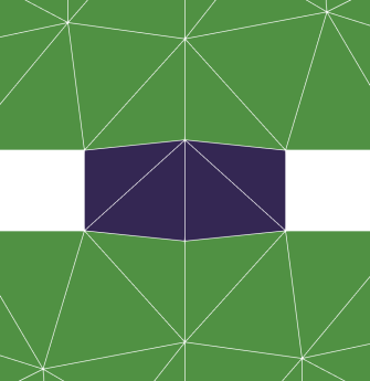
(a) Zoom over the channel with $\delta=1/2^{2}$.

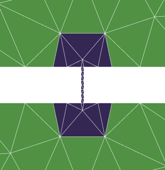
(b) Zoom over the channel with $\delta=1/2^{7}$.

Figure 10: Narrow channel. Zoom of the FE mesh for channel width $\delta=1/2^{2}$ (left) or $1/2^{7}$ (right), with the subdomain $\Omega_{F,\delta}$ (in blue).

Now, we want to decompose $f$ in two terms $f_{F}$ and $f_{S}$ such that as $\delta$ decreases then $\rho_{F}$ increases but $\rho_{S}$ remains constant, where $\rho_{F}$ and $\rho_{S}$ are the spectral radii of the Jacobians of $f_{F}$ and $f_{S}$, respectively. We define a subdomain $\Omega_{F,\delta}$ consisting in the channel plus its neighboring elements having size smaller than the typical mesh size $H$, see Figure 10. Therefore, the size of the elements outside $\Omega_{F,\delta}$ is almost independent of $\delta$. In order to identify $f_{F}$ and $f_{S}$ as the discrete Laplacian inside and outside of $\Omega_{F,\delta}$, respectively, we define a diagonal matrix $D\in\mathbb{R}^{N\times N}$ by $D_{jj}=1$ if $\mbox{supp}(\varphi_{j})\subset\Omega_{F,\delta}$ and $D_{jj}=0$ else. We let

$$f_{F}(X)=DAX,\qquad\qquad f_{S}(t,X)=(I-D)AX+M^{-1}\widehat{b}(t),$$ (5.15)

with $I$ the identity matrix. Thus, as $\delta$ decreases, the size of the elements inside of $\Omega_{F,\delta}$ decrease and $\rho_{F}$ increases, while $\rho_{S}$ is independent of $\delta$.

We will solve 5.12 for varying channel width $\delta$ and investigate the efficiency of the mSK-ROCK and SK-ROCK method. Hence, for each $\delta=1/2^{k}$ with $k=0,\ldots,15$ we solve once

$$\operatorname{d\!}X(t)=f_{S}(t,X(t))\operatorname{d\!}t+f_{F}(X(t))\operatorname{d\!}t+g(X(t))\operatorname{d\!}B(t)\quad t\in(0,T],\qquad\qquad X(0)=0$$ (5.16)

with the mSK-ROCK and SK-ROCK methods, on the same sample path $B(t)$ with $T=0.1$ and the same step size $\tau=0.01$. The relative speed-up $S$ given by the mSK-ROCK scheme over the SK-ROCK method, in terms of CPU time, in function of $\delta$ is displayed in Figure 11(a). For large $\delta$ both methods have the same performance ($S\approx 1$), as $\delta$ decreases the mSK-ROCK becomes more efficient than SK-ROCK and it is at least 25 times faster for some values of $\delta$.

The relative speed-up has been computed dividing the computational costs (CPU time) of the SK-ROCK and mSK-ROCK method, that are plotted in Figure 11(b). This choice is justified by the fact that the relative error between the two solutions, measured in the $L^{2}(\Omega_{\delta})$ norm at time $T$, is less than 1‰, see Figure 11(c). Note that in Figure 11(c) a jump appears exactly when $m$ passes from $m=2$ to $m\geq 4$ (see Figure 11(e)) and thus $r$ passes from $r=1$ to $r\geq 2$. This is due to the fact that for smaller $m$ the mSK-ROCK and SK-ROCK schemes are closer.

The spectral radii $\rho,\rho_{F},\rho_{S}$ of the Jacobians of $f,f_{F},f_{S}$ are shown in Figure 11(d), for large $\delta$ the typical element size is sufficiently small to resolve the channel (Figure 10(a)) and thus $\rho\approx\rho_{F}\approx\rho_{S}$, implying that the costs of mSK-ROCK and SK-ROCK are similar. As $\delta$ decreases then $\rho,\rho_{F}$ increase. Since $\rho_{S}$ is almost constant the number of $f_{S}$ evaluations in the mSK-ROCK method remains constant and only the number of $f_{F}$ evaluations increase, therefore the cost of mSK-ROCK increases less rapidly than the one of SK-ROCK. Finally, in Figure 11(e) we show the number of stages taken by the methods, which reflects the behavior of the spectral radii.

In Figure 11(a) we see a decrease in speed-up for $\delta$ extremely small, this is due to the fact that the cost of evaluating $f_{F}$, with respect to $f_{S}$ and $g$, becomes important; a high number of tiny elements is indeed needed to resolve the channel, hence the total cost $c_{F}+c_{S}+c_{g}=1$ is dominated by $c_{F}$ close to $1$ (see Section 3.2) and this is not the optimal speed-up for the mSK-ROCK method. Nevertheless, the mSK-ROCK scheme still remains about 20 times faster than the SK-ROCK method. We note that in practical applications the mesh outside the channel would also be refined and a value of $c_{F}$ closer to the optimal speed-up could be reached.

(a) Relative speed-up.

(b) Total CPU time w.r.t. $\delta$.

(c) SK-ROCK and mSK-ROCK solutions’ relative error $\|u^{\operatorname{mSK-ROCK}}-u^{\operatorname{SK-ROCK}}\|/\|u^{\operatorname{SK-ROCK}}\|$ in $L^{2}(\Omega_{\delta})$ norm.

(d) Spectral radii w.r.t. $\delta$.

(e) Number of stages.

Figure 11: Narrow channel. Efficiency, evolution of spectral radii and stages.

6 Conclusion

We have introduced a modified equation $\operatorname{d\!}X_{\eta}(t)=f_{\eta}(X(t))\operatorname{d\!}t+g_{\eta}(X(t))\operatorname{d\!}W(t)$ for stiff stochastic differential equations $\operatorname{d\!}X(t)=f_{F}(X(t))\operatorname{d\!}t+f_{S}(X(t))\operatorname{d\!}t+g(X(t))\operatorname{d\!}W(t)$ with different time-scales but without any clear-cut scale separation, where the drift is composed by a stiff but cheap term $f_{F}$ and a mildly stiff but expensive term $f_{S}$. The averaged force $f_{\eta}$ is such that the stiffness of the modified equation depends solely on the slow term $f_{S}$, while the damped diffusion $g_{\eta}$ is such that the mean-square stability properties of the original problem are preserved. Therefore, integration of the modified equation by explicit schemes is cheaper than the original problem, as the stability conditions are not affected by a few severely stiff degrees of freedom in $f_{F}$. Evaluation of both $f_{\eta},g_{\eta}$ requires the solution to fast but cheap deterministic auxiliary problems 2.5 and 2.13, which can be approximated by explicit schemes.

Starting from the modified equation we devised an interpolation-free stabilized explicit multirate scheme, given by 3.10, 3.11, 3.12, 3.13, 3.4 and 3.5. The method consists in integrating the modified equation with a stabilized explicit scheme for SDEs (SK-ROCK) and evaluating $f_{\eta},g_{\eta}$ by solving the auxiliary problems with a stabilized explicit scheme for ODEs (RKC). The scheme, called mSK-ROCK, is fully explicit, has strong order $1/2$, weak order $1$ and it is proven to be stable on a model problem — see Theorems 4.3 and 4.6. The number of expensive function evaluations of $f_{S}$ needed by mSK-ROCK depends only on $f_{S}$ itself; therefore, the efficiency of the scheme is hardly affected by the severely stiff term $f_{F}$.

Furthermore, an important property of the scheme is that it is not based on any scale separation assumption. Therefore, it can be employed for systems stemming from the spatial discretization of stochastic parabolic partial differential equations on locally refined grids, where $f_{F},f_{S}$ represent the Laplacian in refined and coarse regions, respectively (see Section 5.4). Finally, the method is straightforward to implement and numerical experiments demonstrate that the computational cost is significantly reduced without sacrificing any accuracy, compared to the optimal stabilized method for stiff SDEs, namely the SK-ROCK method.

References

- [1] A. Abdulle, I. Almuslimani, and G. Vilmart. Optimal explicit stabilized integrator of weak order one for stiff and ergodic stochastic differential equations. Siam Journal on Uncertainty Quantification, 6(2):937–964, 2018.
- [2] A. Abdulle and S. Cirilli. Stabilized methods for stiff stochastic systems. Comptes Rendus Mathématique. Académie des Sciences. Paris, 345(10):593–598, 2007.
- [3] A. Abdulle and S. Cirilli. S-ROCK: Chebyshev methods for stiff stochastic differential equations. SIAM Journal on Scientific Computing, 30(2):997–1014, 2008.
- [4] A. Abdulle, M. J. Grote, and G. Rosilho de Souza. Explicit stabilized multirate method for stiff differential equations. Technical Report, EPFL, 2020, arXiv:2006.00744 [math.NA].
- [5] A. Abdulle and G. A. Pavliotis. Numerical methods for stochastic partial differential equations with multiple scales. Journal of Computational Physics, 231(6):2482–2497, 2012.
- [6] A. Abdulle, G. A. Pavliotis, and U. Vaes. Spectral methods for multiscale stochastic differential equations. SIAM-ASA Journal on Uncertainty Quantification, 5(1):720–761, 2017.
- [7] A. Abdulle, G. Vilmart, and K. C. Zygalakis. Weak second order explicit stabilized methods for stiff stochastic differential equations. SIAM Journal on Scientific Computing, 35(4):A1792–A1814, 2013.
- [8] J. F. Andrus. Numerical solution of systems of ordinary differential equations into subsytems. SIAM Journal on Numerical Analysis, 16(4):605–611, 1979.
- [9] E. Buckwar and C. Kelly. Towards a systematic linear stability analysis of numerical methods for systems of stochastic differential equations. SIAM Journal on Numerical Analysis, 48(1):298–321, 2010.
- [10] R. Bundschuh, F. Hayot, and C. Jayaprakash. The role of dimerization in noise reduction of simple genetic networks. Journal of Theoretical Biology, 220(2):261–269, 2003.
- [11] Y. Cao, H. Li, and L. R. Petzold. Efficient formulation of the stochastic simulation algorithm for chemically reacting systems. Journal of Chemical Physics, 121(9):4059–4067, 2004.
- [12] D. A. Di Pietro and A. Ern. Mathematical aspects of discontinuous Galerkin methods, volume 69 of Mathématiques et Applications. Springer, Berlin and Heidelberg, 2012.
- [13] W. E. Analysis of the heterogeneous multiscale method for ordinary differential equations. Communications in Mathematical Sciences, 1(3):423–436, 2003.
- [14] W. E, D. Liu, and E. Vanden-Eijnden. Analysis of multiscale methods for stochastic differential equations. Communications on Pure and Applied Mathematics, 58(11):1544–1585, 2005.
- [15] B. Engquist and Y. Tsai. Heterogeneous multiscale methods for stiff ordinary differential equations. Mathematics of Computation, 74(252):1707–1743, 2005.
- [16] C. Engstler and C. Lubich. Multirate extrapolation methods for differential equations with different time scales. Computing, 58(2):173–185, 1997.
- [17] C. W. Gear, G. Ioannis, and G. Kevrekidis. Projective methods for stiff differential equations: problems with gaps in their eigenvalue spectrum. SIAM Journal on Scientific Computing, 24(4):1091–1106, 2003.
- [18] C. W. Gear and D. R. Wells. Multirate linear multistep methods. BIT Numerical Mathematics, 24(4):484–502, 1984.
- [19] D. Givon, I. G. Kevrekidis, and R. Kupferman. Strong convergence of projective integration schemes for singularly perturbed stochastic differential systems. Communications in Mathematical Sciences, 4(4):707–729, 2006.
- [20] A. Guillou and B. Lago. Domaine de stabilité associé aux formules d’intégration numérique d’équations différentielles, à pas séparés et à pas liés. Recherche de formules à grand rayon de stabilité. In 1er Congr. Ass. Fran. Calcul., AFCAL, pages 43–56, Grenoble, 1960.
- [21] M. Günther, A. Kværnø, and P. Rentrop. Multirate partitioned Runge–Kutta methods. BIT Numerical Mathematics, 41(3):504–514, 2001.
- [22] M. Günther and A. Sandu. Multirate generalized additive Runge Kutta methods. Numerische Mathematik, 133(3):497–524, 2016.
- [23] D. J. Higham. An Algorithmic Introduction to Numerical Simulation of Stochastic Differential Equations. SIAM Review, 43(3):525–546, 2001.
- [24] Y. Hu, A. Abdulle, and T. Li. Boosted hybrid method for solving chemical reaction systems with multiple scales in time and population size. Communications in Computational Physics, 12(4):981–1005, 2012.
- [25] I. G. Kevrekidis and A. Papavasiliou. Variance reduction for the equation-free simulation of multiscale stochastic systems. Multiscale Modeling and Simulation, 6(1):70–89, 2007.
- [26] B. S. Kirk, J. W. Peterson, R. H. Stogner, and G. F. Carey. libMesh : a C++ library for parallel adaptive mesh refinement/coarsening simulations. Engineering with Computers, 22(3-4):237–254, 2006.
- [27] H. Kurata, H. El-Samad, T. Yi, M. Khammash, and J. Doyle. Feedback regulation of the heat shock response in E. coli. In Proceedings of the 40th IEEE Conference on Decision and Control, volume 1, pages 837–842, 2001.
- [28] A. Kværnø. Stability of multirate Runge–Kutta schemes. In Proc. of the 10th Coll. on Differential Equations, volume 1A, pages 97–105, 1999.
- [29] B. Lindberg. IMPEX: a program package for solution of systems of stiff differential equations. Technical report, Dept. of Information Processing, Royal Inst. of Tech., Stockholm, 1972.
- [30] D. Liu. Analysis of multiscale methods for stochastic dynamical systems with multiple time scales. Multiscale Modeling and Simulation, 8(3):944–964, 2010.
- [31] G. Milshtein and M. Tretyakov. Stochastic Numerics for Mathematical Physics. Springer, 2003.
- [32] J. R. Rice. Split Runge–Kutta method for simultaneous equations. Journal of research, National Bureau of Standards. Section B, Mathematics and mathematical physics, 64B(3):151–170, 1960.
- [33] S. Roberts, A. Sarshar, and A. Sandu. Coupled Multirate Infinitesimal GARK Schemes for Stiff Systems with Multiple Scales. SIAM Journal on Scientific Computing, 42(3):A1609–A1638, 2020.
- [34] G. Rosilho De Souza. Numerical methods for deterministic and stochastic differential equations with multiple scales and high contrasts. PhD thesis, EPFL, Lausanne, 2020. doi:10.5075/epfl-thesis-7445.
- [35] Y. Saito and T. Mitsui. Stability analysis of numerical schemes for stochastic differential equations. SIAM Journal on Numerical Analysis, 33(6):2254–2267, 1996.
- [36] A. Sandu. A class of multirate infinitesimal GARK methods. SIAM Journal on Numerical Analysis, 57(5):2300–2327, 2019.
- [37] A. Sandu and M. Günther. A generalized-structure approach to additive Runge-Kutta methods. SIAM Journal on Numerical Analysis, 53(1):17–42, 2015.
- [38] V. Savcenco, W. Hundsdorfer, and J. Verwer. A multirate time stepping strategy for stiff ordinary differential equations. BIT Numerical Mathematics, 47(1):137–155, 2007.
- [39] S. Skelboe and P. U. Andersen. Stability properties of backward Euler multirate formulas. SIAM Journal on Scientific and Statistical Computing, 10(5):1000–1009, 1989.
- [40] B. P. Sommeijer, L. Shampine, and J. G. Verwer. RKC: An explicit solver for parabolic PDEs. Journal of Computational and Applied Mathematics, 88(2):315–326, 1998.
- [41] P. J. Van der Houwen and B. P. Sommeijer. On the internal stability of explicit, -stage Runge–Kutta methods for large -values. Zeitschrift für Angewandte Mathematik und Mechanik, 60(10):479–485, 1980.
- [42] E. Vanden-Eijnden. Numerical techniques for multi-scale dynamical systems with stochastic effects. Communications in Mathematical Sciences, 1(2):385–391, 2003.
- [43] E. Vanden-Eijnden. On HMM-like integrators and projective integration methods for systems with multiple time scales. Communications in Mathematical Sciences, 5(2):495–505, 2007.
- [44] J. G. Verwer. An implementation of a class of stabilized explicit methods for the time integration of parabolic equations. ACM Transactions on Mathematical Software (TOMS), 6(2):188–205, 1980.
- [45] J. G. Verwer, W. Hundsdorfer, and B. P. Sommeijer. Convergence properties of the Runge–Kutta–Chebyshev method. Numerische Mathematik, 57(1):157–178, 1990.