Quasinormal modes and their overtones at the common horizon in a binary black hole merger

Abstract

It is expected that all astrophysical black holes in equilibrium are well described by the Kerr solution. Moreover, any black hole far away from equilibrium, such as one initially formed in a compact binary merger or by the collapse of a massive star, will eventually reach a final equilibrium Kerr state. At sufficiently late times in this process of reaching equilibrium, we expect that the black hole is modeled as a perturbation around the final state. The emitted gravitational waves will then be damped sinusoids with frequencies and damping times given by the quasinormal mode spectrum of the final Kerr black hole. An observational test of this scenario, often referred to as black hole spectroscopy, is one of the major goals of gravitational wave astronomy. It was recently suggested that the quasinormal mode description including the higher overtones might hold even right after the remnant black hole is first formed. At these times, the black hole is expected to be highly dynamical and nonlinear effects are likely to be important. In this paper we investigate this remarkable scenario in terms of the horizon dynamics. Working with high accuracy simulations of a simple configuration, namely the head-on collision of two nonspinning black holes with unequal masses, we study the dynamics of the final common horizon in terms of its shear and its multipole moments. We show that they are indeed well described by a superposition of ringdown modes as long as a sufficiently large number of higher overtones are included. This description holds even for the highly dynamical final black hole shortly after its formation. We discuss the implications and caveats of this result for black hole spectroscopy and for our understanding of the approach to equilibrium.

I Introduction

The process of binary black hole coalescence, the formation of a remnant black hole and the associated emission of gravitational waves, provides a rich arena for tests of general relativity (GR). The inspiral regime where we have two distinct black holes inspiralling into each other is well described by the post-Newtonian approximation. A useful framework for tests of general relativity in this regime is provided by the parametrized post-Newtonian framework. It can be argued however that it is the merger regime, which involves the formation of the remnant black hole and its approach to equilibrium, that is the most promising in the search for new physics. It is during the merger that the nonlinear and nonperturbative effects of general relativity are most prominent. Moreover, the approach of the remnant black hole to equilibrium is closely related to one of the important predictions of general relativity, namely the so-called black hole no-hair theorem (see e.g. Chrusciel et al. (2012); Heusler (1996); Cardoso and Gualtieri (2016) for reviews with diverse viewpoints). The final state of the remnant black hole in astrophysical situations is predicted to be a Kerr black hole determined by just two parameters, namely the final mass and angular momentum. When the remnant black hole is initially formed, the spacetime in the vicinity of the horizon is highly dynamical and nonlinear, and it is responsible for the emitted gravitational radiation. In classical general relativity, the horizon itself cannot emit any radiation. Rather, it absorbs part of the emitted radiation to reach equilibrium. The gravitational wave emission at late times during this approach to equilibrium is expected to be described by a superposition of exponentially damped sinusoidal signals, with the frequency and damping times determined just by the final black hole’s mass and angular momentum Vishveshwara (1970); Chandrasekhar and Detweiler (1975); Detweiler (1980) (we can neglect the electric charge for astrophysical black holes). It is an important goal of gravitational wave astronomy to verify (or disprove) this scenario observationally.

Towards this goal, the notion of “black hole spectroscopy” has been proposed Dreyer et al. (2004); Berti et al. (2006, 2016). The basic idea is straightforward: Given that the ringdown frequencies and damping times are determined by just two parameters, if we are able to observe multiple ringdown modes, then the masses and spins inferred from each mode must be consistent. This is then potentially a stringent test of the no-hair theorem; see e.g. Cardoso and Gualtieri (2016) for a more detailed discussion. Moreover, the test applies in principle to any astrophysical process which leads to the formation of a remnant black hole which approaches equilibrium. A binary black hole merger is the obvious target, but it also applies to binary neutron star mergers or the gravitational collapse of sufficiently massive stars. In its original formulation, it was assumed that black hole spectroscopy should only work once the black hole is sufficiently close to equilibrium. Consider for example the remnant black hole formed from a binary black hole merger. When the final black hole is initially formed, it is highly distorted and dynamical, and far from equilibrium. There is thus no a priori reason why the perturbatively defined quasinormal mode frequencies should be associated with the black hole at this point. This issue of isolating the perturbative regime where black hole spectroscopy can be applied is considered e.g. in Thrane et al. (2017).

An important recent development was the suggestion that it might in fact be possible to associate the remnant black hole almost immediately after merger with quasinormal modes Giesler et al. (2019); Isi et al. (2019); Okounkova (2020); see also Jiménez Forteza et al. (2020); Bhagwat et al. (2020); Cook (2020). Given the considerations mentioned at the end of the previous paragraph, this would seem to be a very unlikely proposition. However, as shown in these works, it is clearly true that it is possible to model the gravitational waveform immediately after the merger phase as a superposition of quasinormal modes. For this, it is essential to include the higher ringdown overtones which had, for the most part, not been included in previous analyses. If true, it could greatly improve the prospects of black hole spectroscopy and would indicate a remarkable simplicity in black hole mergers. It is therefore necessary to investigate this scenario from different perspectives, and one such perspective is in the strong field region near the black hole horizons. The goal of this paper is to investigate whether the dynamics of the remnant black hole horizon can be described by a superposition of quasinormal modes (including the higher overtones).

Towards this end, in this paper we carry out a numerical study of the remnant black hole formed by the head-on collision of two nonspinning black holes with unequal masses. This simple configuration, while not of great astrophysical significance, allows one to obtain very accurate numerical relativity simulations. The manifest axisymmetry of such systems also ensures that there is no ambiguity in the choice of coordinate systems and that physical gauge invariant quantities can be extracted in a straightforward manner. The nonlinearities and dynamics of general relativity are of course still present: a common horizon is formed when the two individual black holes get sufficiently close to each other; it settles to a final Schwarzschild black hole, and gravitational radiation is emitted in the process. This provides us with a simple case where the physical question of interest can be fruitfully explored without worrying about many of the complications present in astrophysically realistic situations. Two geometrical quantities related to the final black hole are of interest for our purposes: the angular modes $\sigma_{l}$ ($l=2,3,\ldots$) of the shear $\sigma$ of the outgoing light rays at the horizon, and the nontrivial mass multipole moments $I_{l}$ ($l=2,3,\ldots$) of the horizon. We calculate $\sigma_{l}$ and $I_{l}$ as functions of time and we attempt to describe each of them by a superposition of quasinormal modes. We find that, indeed, including the higher overtones can allow for obtaining excellent fits for $\sigma_{l}(t)$ and $I_{l}(t)$ starting almost immediately after the merger. The high precision of our numerical simulation allows us to include angular modes with $2\leq l\leq 12$, i.e., a total of 11 independent time series, and we show that all of these modes are described by combinations of quas-normal modes provided higher overtones are included. Furthermore, while the multipole moments $I_{l}$ are not fully independent of the shear as we shall see, they do provide yet another 11 functions for testing the hypothesis. Similar studies of the gravitational waves at infinity, e.g. Giesler et al. (2019), typically consider only the dominant $l=|m|=2$ wave mode, with a recent extension to a joint analysis of the $|m|=2$, $l=2,3,4$ wave modes (which are coupled, due to spheroidal/spherical mode mixing in the Kerr final state considered, unlike in our more symmetric case) Cook (2020). Thus, this work represents a significant additional evidence compared to previous work in the literature.

The reader might legitimately ask: i) why should the behavior of $\sigma_{l}$ and $I_{l}$ at the horizon have anything to do with the actual observable quantity, namely the outgoing gravitational waves which could be observed by gravitational wave detectors? Are the horizons not causally disconnected from the outside observers and thus observationally irrelevant? ii) Even if one finds these calculations to be of interest, and even though we are careful in extracting gauge invariant quantities, is the apparent horizon not itself dependent on which time slicing the numerical simulation uses? How can we guarantee that the results would not be entirely different with a different choice of the time coordinate? Let us address these in turn.

For question i), we point out the remarkable correlations that exist between the outgoing radiation seen by a far away observer, and the in-falling radiation that could be seen by a hypothetical observer living near the horizon. Even though these two observers are not in causal contact with each other, the gravitational radiation they would see comes from the same source, namely the nonlinear and time dependent gravitational field in the vicinity of the binary system Jaramillo et al. (2012a, b, 2011); Rezzolla et al. (2010); Gupta et al. (2018). It is thus not a surprise that both observers will see qualitatively similar features. In fact it was shown in Prasad et al. (2020) that the two observations agree qualitatively. The present study can be viewed as further evidence of these correlations. Thus, by studying the behavior of the horizon, we can learn something about the outgoing radiation (and vice versa).

Regarding ii), it is likely true that one could have chosen a particularly “bad” slicing and time coordinate which could have obscured any of the correlations mentioned above. First, we could have made a different choice of spatial Cauchy surfaces for the numerical evolution which would generically lead to different dynamical horizons. Even though there are known constraints on how different the dynamical horizons can be Ashtekar and Galloway (2005), it is possible in principle to choose spatial slices such that the horizons could be extremely distorted Eardley (1998); Ben-Dov (2007). However, we are not aware of any numerical simulations which use, or can practically use, such extreme choices. Second, even within a given choice of slicing, there is still the possibility of choosing a different time parameter adapted to the slicing, $t\mapsto t^{\prime}=F(t)$. This would change the functional dependence of any relevant function of time $f(t)$ into $f^{\prime}(t^{\prime})=f(F^{-1}(t^{\prime}))$. We shall make no attempt to do any such reparametrizations in this paper, and we shall simply work with the slicing and time coordinate used in the simulation.

What is significant is that our results show that there is at least one choice of slicing and of an adapted time coordinate, which happens to be a widely used one, for which the correlations are manifestly present. Specifically, we employ the ${1+\log}$ slicing, along with a $\Gamma$-driver shift condition Alcubierre et al. (2000, 2003). These gauge conditions also set the time parameter and spatial coordinates of the simulation. An important property of these gauge conditions is that they are “symmetry seeking”, i.e., they attempt to find a timelike Killing vector if there is one, and thus define reasonable local observers.

The remainder of the paper is structured as follows. A brief summary of the basic quantities we calculate and study is provided in Sec. II. This section defines and identifies the horizon shear and multipole moments as quantities of interest. In the following sections we describe the methods used and the results of attempts to fit these quantities using the ringdown frequencies and damping times associated with the final black hole. The fitting procedure is described in Sec. III and applied to the shear and multipole moments in Sec. IV. Sec. V discusses the implications of these results and whether it is possible to conclude, and in what sense, whether overtones are really associated with the highly distorted remnant black hole immediately after its formation. Sec. VI concludes with a summary and suggestions for future work.

II Basic notions

There are two main aspects relevant to our study: i) the quasinormal modes (QNMs) of a black hole, which are usually defined within the context of black hole perturbation theory, and ii) the nonperturbative study of quasilocal black hole horizons. This section briefly summarizes the basic notions and results for both of these aspects.

II.1 Quasinormal modes

The metric perturbations of a Schwarzschild black hole (which is the final geometry relevant for our study), for both polar and axial perturbations, can be combined into scalar functions $\psi$ which satisfy equations of the form Regge and Wheeler (1957); Zerilli (1970); Chandrasekhar (1985)

$$\frac{d^{2}\psi}{dr_{\star}^{2}}+\nu^{2}\psi=V_{\pm}\psi\,.$$ ((1))

Here, as usual, $r_{\star}=r+2M\log(r/2M-1)$ with $M$ being the black hole mass, and $r$ is the usual Schwarzschild areal coordinate. The potentials $V_{\pm}$ for the polar and axial perturbations are functions of $r$ and they depend on $M$ and on the mode index $l$. The potentials also differ depending on the nature of the perturbation, and we shall here be concerned almost exclusively with spin-2 fields (see Sec. II.2.3).

Quasinormal modes are obtained by imposing outgoing boundary conditions at both infinity, and at the horizon. Only a discrete set of (complex) values of the frequency $\nu$ allow for these dissipative boundary conditions, and these are labeled by the integers $(l,m,n)$ where $(l,m)$ are the usual angular mode indices in a decomposition into spherical harmonics, and $n=0,1,2,\ldots$ is the overtone index. See Leaver (1985) for an analytic method for calculating this spectrum and Berti ; Berti et al. (2009) for a compilation of the values in different situations. We also show a sample of $m=0$ quasinormal mode frequencies (real and imaginary parts) for a Schwarzschild black hole of unit mass below in Table 1. Finally, there are several interesting mathematical and numerical issues related, in particular, to the non-self-adjoint nature of the problem. For example, of great potential interest is the recent suggestion that the higher overtones might in fact be unstable Jaramillo et al. (2020). Similarly, the issue of the completeness of the quasinormal modes is also of great interest; see e.g. Ansorg and Panosso Macedo (2016); Panosso Macedo et al. (2018); Beyer (1999).

II.2 Nonperturbative framework for studying quasilocal horizons

II.2.1 Horizon definition

The study of horizons here is based on the notions of marginally trapped surfaces and dynamical horizons (see e.g. Ashtekar and Krishnan (2004); Booth (2005); Krishnan (2014); Gourgoulhon and Jaramillo (2006); Faraoni and Prain (2015); Hayward (2000) for reviews). Here we shall only briefly summarize the basic notions required for our purposes. The first is that of a marginally outer trapped surface (MOTS). This is a closed spacelike $2$-surface $\mathcal{S}$ whose outer null-normal $\ell^{a}$ has vanishing expansion:

$$\Theta_{(\ell)}:=q^{ab}\nabla_{a}\ell_{b}=0\,.$$ ((2))

Here $q^{ab}$ is the intrinsic metric on $\mathcal{S}$. MOTSs are closely related to trapped surfaces with negative expansions for both the outgoing and ingoing null normals, and the significance of these notions goes back to the singularity theorems Penrose (1965); Hawking and Penrose (1970). Their presence implies the existence of a spacetime singularity to its future, and thus indicates the presence of a black hole. Well developed methods exist to locate MOTSs in numerical relativity (NR) simulations Thornburg (2007). Here we shall employ the method developed in Pook-Kolb et al. (2019a, b) and available from Pook-Kolb et al. (2020a), which in turn uses libraries described in Schnetter and Miller (2019); Boyle ; Virtanen et al. (2020); van der Walt et al. (2011); Johansson et al. (2018); Meurer et al. (2017); Hunter (2007); Droettboom et al. (2018).

As a MOTS evolves in time, it traces out a $2+1$-dimensional world-tube $\mathcal{H}$ which we shall refer to as a dynamical horizon. Several mathematical and physical properties of $\mathcal{H}$ are known and summarized in the review articles referred to above. The behavior of dynamical horizons in black hole mergers has been studied in detail recently Pook-Kolb et al. (2019c, b, 2020b, 2020c).

II.2.2 Setup and numerical simulation employed

The configuration we consider here is the head-on merger of two nonspinning black holes initially at rest. The initial data is the time symmetric Brill-Lindquist puncture data Brill and Lindquist (1963). This data describes a spatial slice $\Sigma$ with vanishing extrinsic curvature $K_{ab}=0$, and conformally flat 3-metric $h_{ab}=\Phi^{4}\delta_{ab}$. The conformal factor $\Phi$ is a harmonic function on three-dimensional Euclidean space with two points removed (the punctures). At a point $\mathbf{x}$,

$$\Phi(\mathbf{x})=1+\frac{m_{1}}{2r_{1}}+\frac{m_{2}}{2r_{2}}\,,$$ ((3))

where $r_{1,2}$ are the respective distances from $\mathbf{x}$ to each of the two punctures, and $m_{1,2}$ are known as the bare masses of the two punctures. We will note the total Arnowitt Deser Misner (ADM) mass as $M=m_{1}+m_{2}$. We study here a particular configuration with $m_{2}/m_{1}=1.6$. The ADM mass has a value of $1.3$ in the code units used, but we instead set it as the mass unit here, i.e., $M=1$ in this work.

The simulations are carried out based on the Baumgarte-Shapiro-Shibata-Nakamura (BSSN) formulation of the Einstein equations using the Einstein Toolkit Löffler et al. (2012); EinsteinToolkit , with the initial data being generated by TwoPunctures Ansorg et al. (2004). We evolve the spacetime using an axisymmetric version of McLachlan Brown et al. (2009), which uses Kranc Husa et al. (2006); Kranc to generate efficient C++ code. As mentioned earlier, our gauge conditions use a $1+\log$ slicing and a $\Gamma$-driver shift condition Alcubierre et al. (2000, 2003). Further details of our simulation method are described in Pook-Kolb et al. (2019b). The results presented in the present paper use data obtained from a simulation with a spatial grid resolution of ${\rm res}=240$. Additional simulations with resolutions of ${\rm res}=60$, $120,180$, and restricted simulations with higher resolutions of ${\rm res}=480$, $960$, have been used to ensure convergence of our results. We do not use mesh refinement and instead choose our numerical domain large enough to ensure that boundary effects do not reach the horizons up to the final time of $t_{f}\simeq 38.5\,M$ of the simulations.

In the resulting spacetime, we initially have two disjoint MOTSs $\mathcal{S}_{1,2}$. As the time evolution proceeds, $\mathcal{S}_{1}$ and $\mathcal{S}_{2}$ approach each other, touch at a particular time labeled $t_{\rm touch}$, and then go through each other after that. Sometime before $t_{\rm touch}$, at a time labeled $t_{\mathrm{bifurcate}}\simeq 1.06M$, a common horizon forms and immediately bifurcates into two MOTSs representing an outer and an inner branch $\mathcal{S}_{out}$ and $\mathcal{S}_{in}$ respectively. $\mathcal{S}_{in}$ moves inwards, becomes increasingly distorted and eventually merges with $\mathcal{S}_{1}\bigcup\mathcal{S}_{2}$ at $t_{\rm touch}$, and then develops self-intersections. The focus of this paper is not any of these phenomena, but rather the behavior of $\mathcal{S}_{out}$ which moves outwards and loses its distortions as it approaches its final state as that of a spherically symmetric Schwarzschild black hole. We shall in particular look at two particular quantities on $\mathcal{S}_{out}$ as functions of time, namely the shear $\sigma$ of the outward null normal $\ell^{a}$ and the mass multipoles of $\mathcal{S}_{out}$. In the remainder of this section, we shall define these quantities and explain why they are of interest.

II.2.3 Observables on the outer common horizon

We begin with the definition of the shear. Here it will be convenient to introduce a complex basis for tangent vectors on a MOTS: $m^{a}$ and $\bar{m}^{a}$, that satisfy $m\cdot\bar{m}=1$ and $m\cdot m=0$. Then, the shear of the outgoing null normal is defined as

$$\sigma=m^{a}m^{b}\nabla_{a}\ell_{b}\,.$$ ((4))

Such a complex basis is determined up to a spin rotation freedom $m\rightarrow e^{\iota\psi}m$. Under this transformation, the shear transforms as $\sigma\rightarrow e^{2\iota\psi}\sigma$, thus $\sigma$ is said to have spin weight $+2$. This means that $\sigma$ can be expanded in angular modes using spin-weighted spherical harmonics ${}_{2\!}Y_{lm}(\theta,\phi)$ of spin weight $+2$.

There still remains the question of whether there is a preferred choice of angular coordinates $(\theta,\phi)$; we will end up with different mode decompositions for different choices. The general solution to this is given in Ashtekar et al. (2013). (In the present case, since we have manifest axial symmetry, a simpler approach suffices.) On a surface $\mathcal{S}$ of spherical topology equipped with an axial symmetry $\varphi^{a}$, we can introduce preferred angular coordinates $(\theta,\phi)$. First, we assume that $\varphi^{a}$ vanishes at only two points, which are taken to be the poles. On the integral curves of $\varphi^{a}$, take $\phi$ to be the affine parameter along $\varphi^{a}$, normalized to lie in the range $0\leq\phi<2\pi$. One of the meridians, i.e., the lines joining both poles and everywhere orthogonal to $\varphi^{a}$, can be arbitrarily selected. The intersection of this meridian with each integral curve of $\varphi^{a}$ then defines the point on that curve where $\phi$ is set to zero. The other coordinate $\theta$, is defined via $\zeta=\cos\theta$ according to

$$D_{a}\zeta=\frac{4\pi}{A_{\mathcal{S}}}\widetilde{\epsilon}_{ba}\varphi^{b}\,,\quad\oint_{\mathcal{S}}\zeta\,\mathrm{d}A=0\,.$$ ((5))

Here $A_{\mathcal{S}}$ is the area of $\mathcal{S}$, $\widetilde{\epsilon}_{ab}$ is the volume $2$-form, and $D_{a}$ is the covariant derivative compatible with $q_{ab}$. The first equation ensures that $\varphi^{a}D_{a}\zeta=0$. Hence, $\zeta$ is constant on each integral curve of $\varphi^{a}$, and the meridians are integral curves of $D^{a}\zeta$. The second equation fixes the freedom to add an additive constant to $\zeta$ in the first equation. With these choices, it is shown in Ashtekar et al. (2004) that the metric $q_{ab}$ is written as

$$q_{ab}=R_{\mathcal{S}}^{2}\left(\frac{\partial_{a}\zeta\partial_{b}\zeta}{F(\zeta)}+F(\zeta)\,\partial_{a}\phi\partial_{b}\phi\right)\,,$$ ((6))

where $R_{\mathcal{S}}:=\sqrt{A_{\mathcal{S}}/4\pi}$ and

$$F(\zeta)=\frac{4\pi\varphi_{a}\varphi^{a}}{A_{\mathcal{S}}}\,.$$ ((7))

It can be shown that $-1<\zeta<+1$, and it goes from $+1$ to $-1$ as we go from one pole to the other. Therefore we can set $\cos\theta=\zeta$ with $0<\theta<\pi$ (and extend it to $\theta=0$ or $\pi$ at the poles).

We have thus specified $(\theta,\phi)$ on $\mathcal{S}$ (up to a rigid rotation by adding a constant to $\phi$ corresponding to choosing the $\phi=0$ meridian). A suitable choice for $m^{a}$ is given by the following form for its dual $1$-form $\underline{m}$:

$$\underline{m}=\frac{R_{\mathcal{S}}}{\sqrt{2}}\left(\frac{\mathrm{d}\zeta}{\sqrt{F}}+\iota\sqrt{F}\,\mathrm{d}\phi\right)\,.$$ ((8))

We can now expand $\sigma$ as

$$\sigma=\sum_{l}{}_{2\!}Y_{l0}(\theta,\phi)\,\sigma_{l}\,.$$ ((9))

We take only the $(l,0)$ modes because of the manifest axisymmetry. This symmetry and our specific choice for $m^{a}$ also imply here that $\sigma$ and the $\sigma_{l}$ are real. Under time evolution, the mode amplitudes $\sigma_{l}$ will then be real-valued functions of time that we aim to model with a combination of damped sinusoids.

The importance of $\sigma$ lies in the fact that the shear, or more precisely $|\sigma|^{2}$, yields the dominant part of the energy flux in-falling into the black hole Ashtekar and Krishnan (2002, 2003). Based on the discussion in the introduction, we expect the energy fluxes across the horizon to be highly correlated with the outgoing radiation which is determined by the $|\mathcal{N}|^{2}$ with $\mathcal{N}$ being the News function Bondi et al. (1962). Thus one would expect $\sigma$ to be closely correlated with $\mathcal{N}$. This has been shown to be indeed the case for the inspiral regime Prasad et al. (2020). Here our focus is on the postmerger regime. The outgoing radiation is represented by the two polarizations $h_{+,\times}$, or equivalently by a complex combination $h=h_{+}+\iota h_{\times}$. The News function is given by $\mathcal{N}=\dot{h}$. Thus, when $h$ is a combination of damped sinusoids then so is $\mathcal{N}$ and thus, if the proposed correlations mentioned above do exist, the same should be true for $\sigma$. Thus, if the higher overtones appear in $h$, then they should also appear in the shear $\sigma$, and vice versa.

Let us now turn to the multipole moments. As for any mass or charge distribution, it is possible to define suitable mass and current multipoles for black hole horizons Ashtekar et al. (2004). For nonspinning configurations where the individual black holes are nonspinning and the orbital angular momentum is also vanishing, as in our case, we only need to consider the mass multipoles. These are moments $I_{l}$ of the intrinsic scalar curvature $\mathcal{R}$ of $\mathcal{S}$ calculated from Eq. ((6)):

$$I_{l}=\frac{1}{4}\oint_{\mathcal{S}}\mathcal{R}\,Y_{l,0}(\zeta)\,\mathrm{d}A\,.$$ ((10))

Just as for the shear, we calculate $I_{l}$ as functions of time and look for the presence of ringdown modes therein. We will only consider $l\geq 2$ since $I_{0}$ is constant as a topological invariant (here $I_{0}=\sqrt{\pi}$) and $I_{1}$ vanishes at all times due to the symmetries of the angular coordinates used Ashtekar et al. (2004, 2013).

Preliminary investigations of $\sigma_{l}(t)$ and $I_{l}(t)$ are given in Pook-Kolb et al. (2020c). Given that we will analyze essentially the same dataset as in Pook-Kolb et al. (2020c) (here obtained from performing the same simulation with a higher resolution), it will be useful to summarize the results. We begin with plots of $\sigma_{l}$ and $I_{l}$ as functions of time, shown in Fig. 1. The behavior of the modes $\sigma_{l}(t)$ and $I_{l}(t)$ all have similar qualitative behaviors: a rapid initial decay followed by a slower decay with oscillations. The higher the $l$, the more rapid the initial decay. At late times on the other hand, the damping rates of different modes seem very similar, but the higher modes have higher oscillation frequencies. While we shall not discuss it in this paper, we mention in passing that the in-falling energy flux also has a contribution from a vector field $\xi^{a}$ Ashtekar and Krishnan (2002, 2003) (denoted $\zeta^{a}$ in these references). As for the shear, we can perform a mode decomposition for the vector field as well, but using spin-weight-1 spherical harmonics. The time dependence of these modes $\xi_{l}$, $l\geq 1$, is shown in Fig. 2. For $l\neq 2$, it is evidently more complex than the shear. This vector contribution is however subdominant, and we shall study this in detail elsewhere.

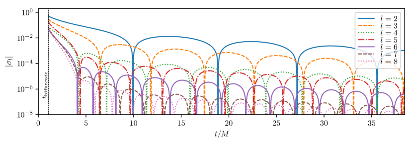
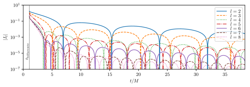
Figure 1: Shear modes (top) and mass multipoles (bottom) for $2\leq l\leq 8$ for $\mathcal{S}_{out}$ as a function of the simulation time. The multipoles $I_{l}$ for $l=0,1$ are constant and not shown. See Sec. II.2.3 for further discussion.

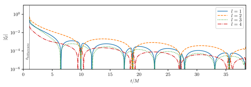
Figure 2: Vector modes $\xi_{l}$ on the outer common horizon for $1\leq l\leq 4$, as a function of the simulation time $t$.

It is also useful to note that the final black hole horizon is not in equilibrium at early times just after it is formed. An easy way to see this is by looking at the area growth of the final black hole. Fig. 3 shows the area of the final black hole as a function of time starting from when it is initially formed. We see a rapid initial increase showing unambiguously the dynamical nature of the black hole in this regime. The analysis of Pook-Kolb et al. (2020c) shows, using many different criteria all of which give approximately the same answer, that the black hole can be considered close to equilibrium after $\sim 10M$ after its formation.

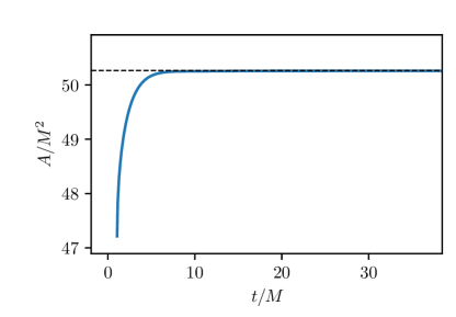
Figure 3: Area of the outer common horizon as a function of simulation time. The final area shown here corresponds to a horizon mass of $\sim(1-7\cdot 10^{-5})\,M$.

It was shown in Pook-Kolb et al. (2020c) that the late-time behavior, on the other hand, is consistent with the principal (fundamental) quasinormal mode. It was also shown there that at early times after the merger, the observed high decay rates were at first glance not consistent with any of the higher overtones considered separately. However, this early-time postmerger behavior analysis was rather simplistic. Here we perform a more sophisticated analysis by considering the entire time series of the shear and multipoles (instead of breaking it up into early and late portions), and model it with a superposition of quasinormal modes including the higher overtones.

We conclude this section with a brief discussion of the relation between the multipoles and the shear. The shear is a spin-weight-2 field, hence it is expanded in spin-weighted spherical harmonics, and it is natural to expect its decay rates to follow the spin-2 quasinormal modes. The scalar 2-curvature of the horizon $\mathcal{R}$, on the other hand, is a spin-weight-0 field which is why Eq. ((10)) uses, in effect, the spin-weight-0 spherical harmonic in defining its moments. Should we then expect the decay rates of $\mathcal{R}$ to follow the spin-0 quasinormal modes? If not, then what should we expect? To answer this question, using the Gauss-Codazzi relations applied to 2-surfaces, we can relate $\mathcal{R}$ to the spacetime Riemann curvature:

$$\mathcal{R}=4\mathrm{Re}[\Psi_{2}]-q^{ac}q^{bd}\sigma^{(\ell)}_{ab}\sigma^{(n)}_{cd}\,.$$ ((11))

Specifically in this paragraph we denote the shear of $\ell^{a}$ (elsewhere simply denoted $\sigma$) with a superscript ^(ℓ) in order to distinguish it from the shear $\sigma^{(n)}$ of the ingoing null normal. $\Psi_{2}$ is a component of the Weyl tensor and $\mathrm{Re}[\Psi_{2}]$ is its real part. We see that $\mathcal{R}$ depends linearly on $\sigma^{(\ell)}$. The shear $\sigma^{(n)}$ is not directly associated with the in-falling radiation, and $\Psi_{2}$ is also not associated with the radiative part of the gravitational field. Thus, $\sigma^{(\ell)}$ controls the time dependence of $\mathcal{R}$, and it is reasonable to expect the decay rates of $\mathcal{R}$ to follow the spin-2 quasinormal ringdown modes. It is also useful to note that for a black hole in equilibrium when there is no in-falling radiation (formally modeled as an isolated horizon Ashtekar et al. (1999, 2000a, 2001, 2002); Lewandowski (2000); Lewandowski and Li (2018); Korzynski et al. (2005); Ashtekar et al. (2000b); Krishnan (2012); Booth (2001, 2013)), the shear $\sigma^{(\ell)}$ vanishes, $\mathcal{R}$ is time-independent and $\mathcal{R}=4\mathrm{Re}[\Psi_{2}]$.

III Overtone models and fitting procedure

In this section we introduce the basic concepts and framework commonly used for the modeling of ringdown-type waveforms (including the outer horizon shear modes and multipoles in our case) with overtones and we the discuss the statistical tools used to fit such models to NR data.

III.1 The overtone model

At late times, we can decompose a spin-weight-$s$ field ${}_{s}X$ propagating in a Schwarzschild (or more generally Kerr) background as a sum of damped sinusoids, namely,

$$_{s}X=\sum_{l\,\geq\,|s|,\,m,\,n}{\mathcal{A}}^{\pm}_{lmn}\,\exp\left[-\iota\omega_{lmn}^{\pm}(t-t_{r})-\frac{t-t_{r}}{\tau_{lmn}^{\pm}}\right]\,_{s\!}\tilde{Y}_{lm}\,.$$ ((12))

Here, the $(l,m)$ indices describe the angular decomposition of the modes (with $m=-l,\dots,l$), and ${}_{s\!}\tilde{Y}_{lm}$ are the spin-weighted spheroidal harmonics; for a perturbed Schwarzschild black hole as in our case, they reduce to the spin-weighted spherical harmonics ${}_{s\!}Y_{lm}$. $n=0,1,2,\dots$ accounts for the $n$-tone excitations of a given $(l,m)$ mode, with $n=0$ being the fundamental “tone” and $n=1,2,\dots$ corresponding to overtones, and $t_{r}$ is a suitable reference time where the linear perturbation theory is expected to describe the dynamics accurately Bhagwat et al. (2018, 2020); Jiménez Forteza et al. (2020); Ota and Chirenti (2020).

If linear perturbation theory applies, the quasinormal mode frequencies and damping times $\omega^{\pm}_{lmn}$ and $\tau^{\pm}_{lmn}$ are solely determined by the black hole’s final mass and angular momentum. For a given choice of the $(l,m,n)$ indices, one finds two families of solutions, those with $\omega_{lmn}^{+}>0$ and those with $\omega_{lmn}^{-}<0$, corresponding to the co-rotating and counter-rotating modes respectively, with their associated damping times $\tau_{lmn}^{\pm}$ and complex amplitudes $\mathcal{A}^{\pm}_{lmn}$ Berti et al. (2006); Leaver (1985); Berti et al. (2009); Kokkotas and Schmidt (1999); Ferrari and Mashhoon (1984); Cook (2020); Jiménez Forteza et al. (2020). Note that for the Schwarzschild case, ${\omega_{lmn}^{+}=-\omega_{lmn}^{-}}$ and ${\tau_{lmn}^{+}=\tau_{lmn}^{-}}$ for any $m$; this also holds in the general Kerr case if $m=0$. Hence, in these cases, the (absolute) values of the frequencies and damping times are independent of the family (co- or counter-rotating) of modes considered.

Throughout this work, we will set $t_{r}$ to the time value used for the late-time fits in Pook-Kolb et al. (2020c), that is in the units used in the present work, $t_{r}/M=20/1.3\simeq 15.4$. The amplitudes at $t_{r}$, ${\cal A}_{lmn}^{\pm}$, are unknown complex numbers that only depend on the perturbation conditions set up during the inspiral-plunge-merger phase of the binary black hole evolution. Hence, they are fully determined by the initial parameters of the binary prior to the merger — in our head-on, nonspinning case, the mass ratio of the two colliding black holes and their relative boost at a given separation.

To allow for deviations on the complex frequencies from the QNM values, Eq. ((12)) may be replaced by

$${}_{s}X=\sum_{l\,\geq\,|s|,\,m,\,n}{\cal A}_{lmn}^{\pm}\,\exp\left[-\iota\omega_{lmn}^{\pm}(1+\alpha_{lmn}^{\pm})(t-t_{r})\right]\times$$

$$\times\exp\left[-\frac{t-t_{r}}{\tau_{lmn}^{\pm}(1+\beta_{lmn}^{\pm})}\right]\,_{s\!}\tilde{Y}_{lm}\,,$$ ((13))

where $\alpha_{lmn}^{\pm}$ and $\beta_{lmn}^{\pm}$ are two sets of perturbation parameters for each co- or counter-rotating mode. These will measure the deviations to the QNM spectrum (as predicted by perturbation theory within GR), while the latter spectrum is recovered for ${\alpha_{lmn}^{\pm}=\beta_{lmn}^{\pm}=0}$. To perform black hole spectroscopy, one shall require a) that the posterior distributions of $\alpha_{lmn}^{\pm}$ and $\beta_{lmn}^{\pm}$ are consistent with zero and b) that the frequency values can be resolved to a given ${n\sigma}$ credible value Bhagwat et al. (2020). The latter is technically difficult due to the low sparsity of the QNM real frequencies. For instance, for the $(l=2,m=0)$ QNM of a ${s=2}$ field in a Schwarzschild spacetime, the real frequencies of the fundamental mode and first overtone only differ by ${1-\omega_{201}^{\pm}/\omega_{200}^{\pm}\simeq 7\%}$ (see the corresponding frequency values in Table 1, left panel), making the separate resolution of the two tone frequencies a challenging task Jiménez Forteza et al. (2020); Bhagwat et al. (2020). An attempt to estimate the overtone frequencies by means of the Bayesian framework on GW150914 data was partially tackled in Isi et al. (2019) by performing a parameter estimation on a reduced parameter space. Other recent studies have provided estimates on the QNM parameters by performing fits to NR data Giesler et al. (2019); Jiménez Forteza et al. (2020); Bhagwat et al. (2020); Cook (2020); Pook-Kolb et al. (2020c). Fitting the data circumvents the extensive exploration of the parameter space by estimating the physical parameters from maximum likelihood estimation algorithms.

The fields originated from head-on collisions of nonspinning black holes —as in our case— are fully described by the $m=0$ modes due to the rotational symmetry of such collisions. In this scenario, all angular ${m\neq 0}$ modes vanish, i.e., ${{}_{s}X_{l,\,m\neq 0,\,n}}=0$. We will only allow for deviations from the QNM spectrum respecting its symmetries, $\omega^{+}_{l0n}=-\omega^{-}_{l0n}$ and $\tau^{+}_{l0n}=\tau^{-}_{l0n}$: i.e., we set $\alpha_{l0n}^{+}=\alpha^{-}_{l0n}$ and $\beta_{l0n}^{+}=\beta^{-}_{l0n}$. Moreover, the fields we are considering, i.e., the multipole moments $I_{l}$, and the shear modes $\sigma_{l}$ as defined above in Sec. II.2.3, are real-valued functions. For such variables, the two families (co- and counter-rotating) of modes combine, with their complex amplitudes at $t_{r}$ satisfying $\mathcal{A}_{l0n}^{-}=(\mathcal{A}_{l0n}^{+})^{*}$, so that

$${\cal A}_{l0n}^{+}\,\exp\left[-\iota\omega_{l0n}^{+}(1+\alpha_{l0n}^{+})(t-t_{r})\right]$$

$$\quad+{\cal A}_{l0n}^{-}\,\exp\left[-\iota\omega_{l0n}^{-}(1+\alpha_{l0n}^{-})(t-t_{r})\right]$$

$$={\cal A}_{l0n}^{+}\,\exp\left[-\iota\omega_{l0n}^{+}(1+\alpha_{l0n}^{+})(t-t_{r})\right]$$

$$\quad\;+\left({\cal A}_{l0n}^{+}\right)^{*}\,\exp\left[+\iota\omega_{l0n}^{+}(1+\alpha_{l0n}^{+})(t-t_{r})\right]$$

$${}=A_{l0n}\,\cos\left[{\omega_{l0n}^{+}(1+\alpha_{l0n}^{+})\,(t-t_{r})+\phi_{l0n}}\right]\,,$$

with $\mathcal{A}_{l0n}^{+}\equiv(1/2)\,A_{l0n}\exp\left[-\iota\phi_{l0n}\right]$ and for a real amplitude $A_{l0n}$ and phase $\phi_{l0n}$. With the above remarks, from now onwards we can drop the ^± superscripts on all parameters and simplify the ansatz of Eq. (III.1) into,

$${}_{s}X_{l0}(t)=\sum_{n=0}^{n_{\mathrm{max}}} \;A_{l0n}\,\exp\left[-\frac{t-t_{r}}{\tau_{l0n}(1+\beta_{l0n})}\right]\times$$

$$\quad\times\cos\left[{\omega_{l0n}(1+\alpha_{l0n})(t-t_{r})+\phi_{l0n}}\right]\,,$$ ((14))

with ${}_{s}X_{l0}=\mathrm{Re}({}_{s}X_{l0})$. As a sign flip on the real frequencies would still be possible in principle, we specify that the co-rotating (positive real part) choice is implied for the complex frequencies $\nu_{l0n}$ and their real part $\omega_{l0n}$. We will further drop the fixed $s=2$ and $m=0$ subscripts on $X_{l}\equiv{}_{s}X_{l0}$ in the following.

The parameters $\alpha_{l0n}$ and $\beta_{l0n}$ help one test the effects of eventual systematic errors sourced by a) including an insufficient number of tones $n_{\mathrm{max}}$ when modeling the data with Eq. (III.1) or b) the presence of non-negligible nonlinearities in the data Bhagwat et al. (2018, 2020); Jiménez Forteza et al. (2020). We note in passing that introducing the parameters $\alpha_{l0n}$ and $\beta_{l0n}$ may also be used in a more general context to parametrize deviations from general relativity.

In this work we model the data for the shear modes $\sigma_{l}$ and multipoles $I_{l}$ with $2\leq l\leq 12$, using multiple values of $n_{\mathrm{max}}$, up to $n_{\mathrm{max}}=15$. In general, we fit for the amplitude $A_{l0n}$ and for the phase $\phi_{l0n}$, and we either set the frequency deviation parameters $\beta_{l0n}$ and $\alpha_{l0n}$ to zero or additionally fit for them.

We compute the QNM spectrum values $\{\omega_{l0n},\tau_{l0n}\}$ of the final black hole using the qnm Python script Stein (2019), which combines a Leaver solver with the Cook-Zalutskiy spectral approach to the angular sector Leaver (1985); Cook and Zalutskiy (2014). Our final black hole has no spin and its mass is slightly lower than $M$ due to the gravitational radiation. This relative mass decrease with respect to $M$ can be estimated at about $7\cdot 10^{-5}$ from the outer horizon area at late times. We simply approximate the final mass as $M$ when computing the QNM spectrum, implying a similar relative error on $\tau_{l0n}$ and $\omega_{l0n}$ which are proportional and inversely proportional to the final mass, respectively. In Table 1, we show as an example, a sample of the resulting QNM frequencies $\omega_{l0n}$ and damping rates $1/\tau_{l0n}$, for $l=2,\dots,12$ and $n=0,\dots,5$.

l	n=0	n=1	n=2	n=3	n=4	n=5
2	0.3737	0.3467	0.3011	0.2515	0.2075	0.1693
3	0.5994	0.5826	0.5517	0.5120	0.4702	0.4314
4	0.8092	0.7966	0.7727	0.7398	0.7015	0.6616
5	1.0123	1.0022	0.9827	0.9550	0.9211	0.8833
6	1.2120	1.2036	1.1871	1.1633	1.1333	1.0988
7	1.4097	1.4025	1.3882	1.3674	1.3407	1.3093
8	1.6062	1.5998	1.5872	1.5687	1.5449	1.5163
9	1.8018	1.7961	1.7848	1.7682	1.7466	1.7205
10	1.9968	1.9916	1.9815	1.9664	1.9467	1.9227
11	2.1913	2.1866	2.1773	2.1635	2.1455	2.1234
12	2.3855	2.3812	2.3727	2.3600	2.3433	2.3228

l	n=0	n=1	n=2	n=3	n=4	n=5
2	0.0890	0.2739	0.4783	0.7051	0.9468	1.1956
3	0.0927	0.2813	0.4791	0.6903	0.9156	1.1522
4	0.0942	0.2843	0.4799	0.6839	0.8982	1.1230
5	0.0949	0.2858	0.4803	0.6806	0.8882	1.1042
6	0.0953	0.2866	0.4806	0.6786	0.8821	1.0921
7	0.0955	0.2872	0.4807	0.6773	0.8782	1.0841
8	0.0957	0.2875	0.4808	0.6765	0.8755	1.0786
9	0.0958	0.2877	0.4809	0.6759	0.8736	1.0747
10	0.0959	0.2879	0.4809	0.6755	0.8723	1.0718
11	0.0959	0.2880	0.4810	0.6752	0.8712	1.0696
12	0.0960	0.2881	0.4810	0.6749	0.8704	1.0679

Table 1: QNM real frequencies $\omega_{l0n}\equiv\left|\omega_{l0n}^{\pm}\right|=\left|\mathrm{Re}(\nu_{l0n}^{\pm})\right|$ (left) and damping rates $1/\tau_{l0n}\equiv 1/\tau_{l0n}^{\pm}=-\mathrm{Im}(\nu_{l0n}^{\pm})$ (right) for a Schwarzschild black hole with unit mass, for $l=2,\dots,12$ and $n=0,\dots,5$, computed with the qnm Python script Stein (2019).

The fitting algorithm is explained in Sec. III.2. In Sec. IV.1 we explore the fit results for a single-tone ($n_{\mathrm{max}}=0$) analysis. We observe that the single-tone model is not sufficient to fully describe even the late-time data. In Sec. IV.2 we extend the results to the multiple-tone ($n_{\mathrm{max}}>0$) analysis and to the whole dataset, with all the $\alpha_{l0n}$ and $\beta_{l0n}$ parameters set to zero. In this case and for large enough $n_{\mathrm{max}}$, we find that the model is sufficient to describe the data even including the early times where the horizon is not in equilibrium. In Sec. V we discuss this, and investigate whether one can infer from it an actual presence and predominance of overtones over nonlinear contributions right from shortly after the horizon is formed.

III.2 The fitting algorithm

We use a maximum likelihood estimation algorithm to obtain the best-fit parameters $\lambda_{i}$. Those correspond to the parameter values that minimize the $\chi^{2}$, namely,

$$\chi^{2}=\sum_{k}\left|h_{x}\left[\vec{\lambda}\right](t_{k})-h_{\mathrm{NR}}(t_{k})\right|^{2},$$ ((15))

where $h_{x}\left[\vec{\lambda}\right]$ stands for the model given by Eq. (III.1) and evaluated at the parameters $\vec{\lambda}=\left\{A_{l0n},\phi_{l0n}\right\}$ or $\vec{\lambda}=\left\{A_{l0n},\phi_{l0n},\alpha_{l0n},\beta_{l0n}\right\}$, and $h_{\rm NR}=\left\{\sigma_{l},I_{l}\right\}$ stands for the numerical data for the shear modes or multipoles, respectively. We sum over the data points $k$ at all times $t=t_{k}\in[t_{0},t_{f}]$, for a certain fit starting time $t_{0}$ which may be picked at any value $t_{\mathrm{bifurcate}}\leq t_{0}\leq t_{f}$, and where, as above, $t_{f}\simeq 38.5M$ is the end time of the simulation. Minimization of ((15)) is performed running the Levenberg-Marquardt algorithm for nonlinear fitting as implemented in Mathematica Inc. .

To assess the fit goodness we use the mismatch $\mathcal{M}$ as in Giesler et al. (2019); Bhagwat et al. (2020); Jiménez Forteza et al. (2020); Cook (2020), which is defined as

$$\mathcal{M}=1-\frac{\langle h_{\rm NR}|h_{x}\rangle}{\sqrt{\langle h_{\rm NR}|h_{\rm NR}\rangle\langle h_{x}|h_{x}\rangle}}\,$$ ((16))

with

$$\langle f|g\rangle=\int_{t_{0}}^{t_{f}}f(t)g(t)\,\mathrm{d}t\,.$$ ((17))

The standard errors $\delta\lambda_{i}$ on the parameters are computed from the diagonal terms of the covariance matrix as Inc. ,

$$\delta\lambda_{i}=\sqrt{\frac{2\,\text{RSS}\times[H^{-1}]_{ii}}{N-p}}\,,$$ ((18))

where $[H^{-1}]_{ii}$ stands for the diagonal terms of the $[H^{-1}]_{ij}$ matrix (without implicit summation on the $i$ indices);

$$\text{RSS}=\sum_{k}\big{(}h_{NR}(t_{k})-h_{x}(t_{k})\big{)}^{2}$$ ((19))

is the residual sum of squares; $N$ is the number of data points in the time range considered, i.e. in $[t_{0},t_{f}]$; and $p$ is the number of parameters one wants to fit for. $H_{ij}$ is the Hessian matrix defined as

$$H_{ij}=\frac{\partial^{2}(\text{RSS})}{\partial\lambda_{i}\,\partial\lambda_{j}}\Bigm{|}_{\vec{\lambda}}\;\;,$$ ((20))

which is evaluated at the best fit parameters $\vec{\lambda}$.

III.3 Exponential rescaling procedure and numerical errors

The NR data appears to be exponentially damped at late times, and so are the damped-sinusoidal models of the class (III.1) that we fit to this data. Due to this damping, the fitting procedure based on the residual sum of squares —rather than relative differences— will capture better the behavior of the NR data towards the beginning of the time interval considered (close to $t_{0}$) than towards the latest times (close to $t_{r}$). A reliable estimate of the oscillation frequencies, damping rates, and amplitudes of each tone in the model would rather require an accurate match of the relative amplitudes and positions of the successive extrema (or zeros), and thus a small relative deviation to the NR data, on the entire time interval considered.

To this aim, when looking specifically for the best-fit frequencies, damping rates and/or amplitudes, we will first apply a time-dependent rescaling of the NR data and of the model, determined by the damping rate of the fundamental QNM. That is, we will fit a rescaled dataset with the similarly rescaled model according to

$$h_{\mathrm{NR}}(t) \mapsto\tilde{h}_{\mathrm{NR}}(t)=\exp\left[+\frac{t-t_{r}}{\tau_{l00}}\right]\,h_{\mathrm{NR}}(t)\;;$$

$$h_{x}(t) \mapsto\tilde{h}_{x}(t)=\exp\left[+\frac{t-t_{r}}{\tau_{l00}}\right]\,h_{x}(t)\;,$$ ((21))

where the unrescaled model $h_{x}(t)$ is given by Eq. (III.1) for a certain $n_{\mathrm{max}}$, and with the parameters $\alpha_{l0n}$ and $\beta_{l0n}$ either set to zero, or left as free parameters. In this way, provided the late-time decay rate of the NR data is comparable to the fundamental QNM value on the time range considered, the rescaled dataset will have an approximately constant (rather than decaying) amplitude towards late times. This then allows for a more accurate retrieval of the complex frequency parameters $\alpha_{l0n}$ and $\beta_{l0n}$, if left free, and of the amplitudes $A_{l0n}$.

Such a rescaling will of course also scale up the numerical errors at late times. However, the high resolution used here means that the relative error on the computed shear modes and multipoles remains rather low for all modes $l\leq 12$. We conservatively estimate the error on the NR results —assuming it to be dominated by discretization error— as the difference between the values obtained at the highest resolution, $\mathrm{res}=240$ —used throughout this paper— and the next highest resolution available, $\mathrm{res}=180$. The relative error on the shear modes and multipoles computed in this way increases with $l$ as the amplitude of the modes decreases. Away from the zeros of the modes, it ranges from about $10^{-6}$ at $l=2$ to about $1\%$ at $l=12$ for the shear modes, and up to $1$ order of magnitude larger for the multipoles. We accordingly consider $l=12$ as a threshold value for sufficiently small numerical uncertainties and we shall not consider the higher-$l$ modes in the present work. Fig. 4 shows the rescaled NR data $\tilde{h}_{\mathrm{NR}}$ and the numerical error on this rescaled data as a function of time for the two extreme cases of the smallest ($\sigma_{2}$, left panel) and the largest ($I_{12}$, right panel) relative error among the modes we consider.

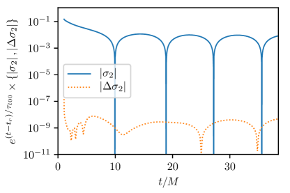
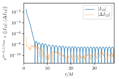
Figure 4: Left: rescaled highest-resolution NR results for the shear $l=2$ mode (continuous line) and numerical error on this rescaled dataset evaluated as the difference with the next-highest resolution available (dashed line; see Sec. III.3), as a function of simulation time. Right: same results for the $l=12$ multipole. These two cases represent respectively the smallest and the largest relative numerical errors among the modes considered in this analysis.

IV Fit results

IV.1 Single-mode fits with variable frequency and damping rate

Before considering higher overtones, we first focus on the $s=2$ fundamental QNMs of the remnant black hole. We aim at checking whether we recover the good agreement found in Pook-Kolb et al. (2020c) (with a different method as used here) between the damped oscillating behavior of the shear modes and multipoles at late times on the one hand, and the complex frequencies of these fundamental modes on the other hand.

To this end, we consider a single-tone model where the frequency and damping rate are free parameters, i.e., the ringdown model (III.1) restricted to the $n=0$ fundamental tone:

$$X_{l}(t)=A_{0}\exp\left[-\frac{t-t_{r}}{\tau_{l\,00}(1+\beta_{0})}\right]\cos\left[(1+\alpha_{0})\,\omega_{l00}(t-t_{r})+\phi_{0}\right].$$ ((22))

We will then check to what extent the best-fit frequencies and damping times in such a model match the fundamental QNM values, corresponding to $\alpha_{0}=0$ and $\beta_{0}=0$, for the late-time shear modes and multipoles. Thanks to the high numerical resolution, we can perform this analysis up to the $l=12$ mode of the shear and multipoles, so that we can also consider whether the conclusions of Pook-Kolb et al. (2020c) on the late-time behavior of these variables do extend beyond the $l=7$ mode.

Note that for convenience, we here drop the $l$ and the $m=0$ indices on the free parameters, that is on $A_{0}\equiv A_{l00}$, $\phi_{0}\equiv\phi_{l00}$, $\alpha_{0}\equiv\alpha_{l00}$ and $\beta_{0}\equiv\beta_{l00}$. It should however be understood that their values will, of course, depend on the variable $X_{l}$ considered, i.e., on the observable $X$ (shear or multipoles) and on the mode $l$.

IV.1.1 Late-time best-fit frequencies and comparison to the fundamental QNM values

We first turn our attention to the late-time data as selected in the same way as in Pook-Kolb et al. (2020c), i.e., we consider $t\in[t_{0},t_{f}]$ for $t_{0}/M=20/1.3\simeq 15.4$. (In this case, the fit starting time $t_{0}$ then coincides with the constant value we have set for $t_{r}$.)

We begin by considering the shear modes $\sigma_{l}$ for $2\leq l\leq 12$. Fig. 5 shows the best-fit values for each mode $l$ for the real (left panel) and imaginary (right panel) parts of the model’s single frequency $\nu=(1+\alpha_{0})\,\omega_{l00}-\iota\,\tau_{l00}^{-1}(1+\beta_{0})^{-1}$, using the rescaling procedure ((21)) to obtain a better accuracy in the recovery of $\nu$. The results for $\mathrm{Re}(\nu)$ and $\mathrm{Im}(\nu)$ are normalized to the corresponding fundamental QNM values, and we also include as error bars on these results, the $1\sigma$ (standard) deviations on the best-fit estimates as computed from the covariance matrix using Eq. ((18)) (see Sec. III.2). The results from Pook-Kolb et al. (2020c) are also indicated for comparison when available, i.e., for $l\leq 7$.

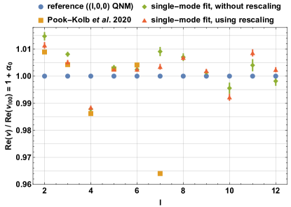
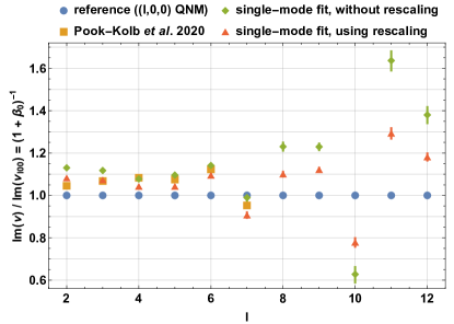
Figure 5: Best-fit real (left) and imaginary (right) frequencies for the shear $l=2$ to $l=12$ modes obtained for $t_{0}=(20/1.3)\,M$ using the single-mode model of Eq. ((22)) and the rescaling procedure given by Eq. ((21)), shown as red triangles with $1\sigma$ error bars (computed from Eq. ((18))). The values are normalized to the fundamental QNM values and the reference unity value for this ratio is marked as blue disks. The best-fit values we obtain without using the rescaling procedure are also shown for reference (green diamonds) with their associated $1\sigma$ uncertainties, and the values quoted from Pook-Kolb et al. (2020c) for $l\leq 7$ are also given for comparison (orange squares). For the latter, we do not show error bars on the figure as precise uncertainties were not given for every $l$. These uncertainties were estimated to be of the order of $\delta(\mathrm{Re}(\nu))/\mathrm{Re}(\nu)\simeq\pm 1\%$ for the real part and $\delta(\mathrm{Im}(\nu))/\mathrm{Im}(\nu)\simeq\pm 10\%$ for the imaginary part for each $l\leq 6$, and larger for $l=7$.

For the real part, we find that the relative deviations to the fundamental QNM values, $\mathrm{Re}(\nu)/\mathrm{Re}(\nu_{l00})-1=\alpha_{0}$, stay within $\pm 1.5\%$ for all modes $l\leq 6$, in agreement with Pook-Kolb et al. (2020c). We extend this conclusion to $7\leq l\leq 12$ with deviations ${|\alpha_{0}|}$ below $\sim 1\%$ in these cases (while a deviation of about ${\alpha_{0}\simeq-3.6}\%$ was found in Pook-Kolb et al. (2020c) for $l=7$, with a larger uncertainty). We also obtain deviations $\left|\,\mathrm{Im}(\nu)/\mathrm{Im}(\nu_{l00})-1\right|$ within $\sim 10\%$ to the fundamental QNM values for the imaginary part for $l\geq 7$, in consistency with  Pook-Kolb et al. (2020c).

The disagreement to the QNM values for the imaginary part does however increase for larger values of $l$, up to the order of $\left|\,\mathrm{Im}(\nu)/\mathrm{Im}(\nu_{l00})-1\right|\simeq 20\%$ to $\sim 30\%$ for $l=10$, $11$ and $12$. For these large-$l$ modes the quasinormal fundamental mode is thus no longer an accurate model of the shear modes for the range $t\gtrsim 15.4M$, at least regarding their damping rates. The $\left|\,\mathrm{Im}(\nu)/\mathrm{Im}(\nu_{l00})-1\right|\simeq 10\%$ deviations at several of the smaller-$l$ values despite uncertainties much smaller than this number suggest that this may even be the case for most of the modes. This may be a consequence of the presence of residual nonlinear deviations to equilibrium at these times, or of the residual presence of higher overtones for these modes. The latter hypothesis would explain the larger decay rates found for most modes and the very small deviations on the real parts of the frequencies: the respective real frequencies $\omega_{l01}$ and $\omega_{l00}$ of the QNM first overtone and fundamental mode differ by ${1-\omega_{201}/\omega_{200}\simeq 7}\%$ for $l=2$ and by even smaller amounts for all higher-$l$ modes, while the decay rates of the QNM first overtones are typically $3$ times larger than those of the fundamental modes (see Table 1). The decay rates smaller than the fundamental QNM value found for $l=7$ and $l=10$ would be harder to explain in this scenario, but could be caused by a modulation induced by a higher overtone if this latter is nearly in antiphase with the fundamental mode. This would cause a decrease in the overall amplitude in the early part of the time range considered (i.e., for $t$ close to $t_{0}$) before the overtone fully decays away.

Note that the systematics due to the errors in the numerical data are not included in the error bars shown. We can estimate these errors by comparing the best-fit frequencies to those found by instead fitting the (rescaled) next-highest-resolution ($\mathrm{res}=180$) NR data. The relative deviations $\Delta(\mathrm{Re}(\nu))/\mathrm{Re}(\nu)$, $\Delta(\mathrm{Im}(\nu))/\mathrm{Im}(\nu)$ obtained in this way on the best-fit real and imaginary frequencies are very small for the low values of $l$. They remain under $10^{-4}$ for all modes for the real part, and under $10^{-3}$ for all modes for the imaginary part. There are further systematic errors if, e.g., nonlinearities or higher overtones are present since they are not accounted for in the model.

For comparison, we also include in Fig. 5 the results obtained from directly fitting the model ((22)) to the NR data on the same time range, this time without applying the rescaling ((21)). For the real frequency $\mathrm{Re}(\nu)$, these results remain within $\pm 1.5\%$ of the QNM values $\omega_{l00}$ for all modes. They however display substantial systematic errors with much larger deviations to the QNM values $\mathrm{Im}(\nu_{l00})$ for the imaginary parts $\mathrm{Im}(\nu)$ for almost all modes, due to an inaccurate fitting of the decaying amplitude over time.

We then repeat this analysis for the multipole moments $I_{l}$ for $2\leq l\leq 12$. The results are shown in Fig. 6 where the available ($l\leq 7$) results from Pook-Kolb et al. (2020c) for the multipoles are again also given for comparison. As also found in the latter reference, the results we obtain for the multipoles are qualitatively very similar to those obtained for the shear modes. We here again focus on the results obtained after applying the rescaling procedure given by Eq. ((21)), which is expected to improve the determination of the frequencies.

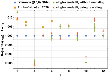
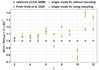
Figure 6: Same as Fig. 5, for the successive multipoles $I_{2}$ to $I_{12}$.

The real frequencies $\mathrm{Re}(\nu)$ again remain within $\pm\sim 1.5\%$ (although no longer within $\pm\sim 1\%$ at large $l$ values) of the fundamental QNM real frequencies $\mathrm{Re}(\nu_{l00})=\omega_{l00}$. The imaginary frequencies $\mathrm{Im}(\nu)$ still feature relative deviations to the QNM values $\mathrm{Im}(\nu_{l00})=\tau_{l00}^{-1}$ of up to $\pm\sim 10\%$ for $l\leq 9$ and larger deviations for $l\geq 10$, although they do remain below $\sim 20\%$ in magnitude for all modes. While these magnitudes do change, we note that the signs of the deviations $\mathrm{Im}(\nu)/\mathrm{Im}(\nu_{l00})-1$ are the same as those found for the shear for every mode $l$.

The numerical relative errors on the best-fit frequency values, estimated in the same way as for the shear above, are again very small at small $l$. They reach slightly larger values than for the shear, from $\Delta(\mathrm{Re}(\nu))/\mathrm{Re}(\nu)\sim 1\cdot 10^{-3}$ to just above $2\cdot 10^{-3}$, for the real frequencies and $l=10$ to $12$. For the imaginary part, these relative error estimates stay below $\Delta(\mathrm{Im}(\nu))/\mathrm{Im}(\nu)\sim 10^{-3}$, as for the shear, for $l\leq 9$; but they reach about $4$ to $9\cdot 10^{-3}$ for the last three modes, implying a small but non-negligible possible systematic error on the values of $\mathrm{Im}(\nu)/\mathrm{Im}(\nu_{l00})$ shown in these cases.

Note that the QNM complex frequencies used here are still those of a field of spin-weight $2$, as for the shear. The late-time oscillations of the multipoles match well the corresponding real frequencies (as well as the damping rates to a lesser extent), even though —unlike the spin-weight-$2$ shear scalar— the multipoles are scalar fields of spin weight $0$. For instance, the fundamental $l=2$ QNM real frequency for a spin-0 perturbation is nearly $30\%$ larger than the corresponding frequency for spin-2 perturbations; a difference which would be easily noticeable. Hence, the dynamics of the geometry of the outer common horizon as measured by the mass multipoles may be determined by the shear flux at the horizon, at least at the late times considered so far. This is entirely consistent with the discussion at the end of Sec. II.2.3.

IV.1.2 Dependence on the fit starting time

We can also let the fit starting time $t_{0}$ vary and span the available interval $[t_{\mathrm{bifurcate}},t_{f}]$. One can expect the behavior of the shear scalar and multipoles to be fully described by the fundamental QNM $(n=0)$ at large $t$, i.e., in the near-equilibrium regime and after the higher overtones have decayed away. If this is the case, the best-fit complex frequencies to the shear modes and to the multipoles should converge towards the fundamental QNM values at late times.

Fig. 7 shows the best-fit complex frequency deviation parameters $\alpha_{0}$ and $\beta_{0}$ for the time range $[t_{0},t_{f}]$ as a function of $t_{0}$, for the shear $l=2$ mode as an example, along with $1\sigma$ uncertainties on these parameters as given by Eq. ((18)). The rescaling given by Eq. ((21)) has again been applied to the model and to the NR data for a more accurate retrieval of the complex frequency. The results similarly obtained for the $l=2$ multipole are shown in Fig. 8 —still using the $s=2$ fundamental QNM as the reference complex frequency value— with very similar behaviors. In both cases, both parameters $\alpha_{0}$ and $\beta_{0}$ do appear to converge towards zero, or at least to a value of modulus $|\beta_{0}|<10^{-2}$ in the case of $\beta_{0}$, as $t_{0}$ approaches $t_{f}$.

Figure 7: Best-fit parameters $\alpha_{0}$ (blue) and $\beta_{0}$ (orange) as functions of the fit starting time $t_{0}$, for the shear $\sigma_{2}$ mode and for the single-tone model ((22)). The rescaling procedure ((21)) has been applied prior to fitting. $1\sigma$ deviations (Eq. ((18))) around the best-fit values are included.

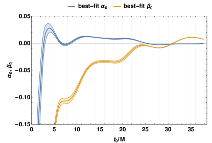
Figure 8: Same as Fig. 7, for the $I_{2}$ multipole.

However, $\alpha_{0}$ and —more prominently— $\beta_{0}$ clearly deviate from zero for earlier fit starting times. In particular, $\beta_{0}$ reaches increasingly negative values, corresponding to larger and larger damping rates, as $t_{0}$ is decreased. Such deviations are of course expected at early times when nonlinear deviations to equilibrium should still be present. The observed behavior of $\alpha_{0}$ and $\beta_{0}$ is however also compatible with the presence of QNM overtones, which are damped faster than the fundamental mode. Their presence may indeed be expected at least at the intermediate times $t/M\simeq 10$ to $20$, if the nonlinear dynamics have become sufficiently negligible, and before these overtones have decayed much below the fundamental mode.

The best-fit $\alpha_{0}$ and $\beta_{0}$ values for the higher shear modes and multipoles typically display similar behaviors as those observed here for $l=2$, although the residual magnitudes of these quantities towards $t_{f}$ can be a little larger than in the $l=2$ case, with $|\alpha_{0}|\lesssim 1\%$ and $|\beta_{0}|\lesssim 5\%$, and with typically $\alpha_{0}<0$ and $\beta_{0}>0$. For both the shear and multipoles, the $l=7$ and $l=10$ modes (already singled out in Figs. 5 and 6 for their atypical best-fit damping rates) are exceptions regarding the best-fit $\beta_{0}$, which takes again substantial positive values (ranging from $\beta_{0}\simeq 0.18$ to $\beta_{0}\simeq 0.37$) for very late starting times $30M\lesssim t_{0}<t_{f}$ —where few data points remain— after being first damped with increasing $t_{0}$ for $t_{0}\lesssim 30M$.

IV.2 QNM models including overtones

In the previous subsection, we noted that the late-time oscillations of each of the shear modes and multipoles for $2\leq l\leq 12$ were well modeled by the real frequency $\omega_{l00}$ of the corresponding $s=2$ fundamental QNM of the remnant black hole. On the other hand, the damping rates of these oscillations showed some deviation to the fundamental QNM imaginary frequencies $\tau_{l00}^{-1}$, especially at large $l$. Moreover, the deviations on both the real and the imaginary frequencies generally appeared to increase as earlier times were taken into account, and to nearly vanish if only the very end of the dataset was considered. We have accordingly suggested that the shear modes and multipoles are fully described asymptotically by the fundamental QNMs while the behavior at more intermediate times (say, around $t=15M$) may correspond to the additional residual presence of higher overtones.

Moreover, as already pointed out in Pook-Kolb et al. (2020c), each of the shear modes and multipoles clearly displays a steep nonoscillating decay at early times (at $t/M\lesssim 4$), with a substantially larger damping rate than the late-time damped-oscillatory regime. Accordingly, none of the modes can be correctly described by a single damped sinusoid over the whole time range $[t_{\mathrm{bifurcate}},t_{f}]$. It was noted in Pook-Kolb et al. (2020c) that the larger decay rate observed at early times, while reminiscent of the large values of the imaginary frequencies of the QNM overtones, generally did not appear to quantitatively match the imaginary frequency of any particular overtone. It was left as a possibility that this early damping regime may nevertheless correspond to combined contributions of multiple overtones.

Accordingly, we will now examine the hypothesis that the behavior of each of the outer common horizon shear modes and multipoles is consistently described by a combination of QNMs, including overtones, over the whole available time range from the very formation of this horizon or shortly afterwards. To this end, we consider the multiple-tone model given by Eq. (III.1) with all complex frequencies set to the QNM values, i.e., $\alpha_{l0n}=\beta_{l0n}=0\;\forall l,n$:

$$X_{l}=\sum_{n=0}^{n_{\mathrm{max}}}A_{n}\,\exp\left[-\frac{t-t_{r}}{\tau_{l0n}}\right]\,\cos\left[\omega_{l0n}(t-t_{r})+\phi_{n}\right]\;,$$ ((23))

where we have again dropped the $m=0$ index and the implicit $l$ dependence on the free parameters: $A_{n}\equiv A_{l0n}$ and $\phi_{n}\equiv\phi_{l0n}$. We then check for the agreement of such a combination of QNMs to the numerically computed shear modes and multipoles as the total number $n_{\mathrm{max}}$ of overtones is varied.

We here aim at directly comparing the above class of models to the NR results, rather than at accurately estimating best-fit frequencies or amplitudes. Accordingly, for a more straightforward comparison and interpretation, in this subsection we will directly use the models and NR datasets without applying a rescaling procedure such as that of Eq. ((21)).

IV.2.1 Shear modes

We first consider the shear modes $\sigma_{l}$, with, as in the previous subsection, $2\leq l\leq 12$. We begin by considering, for each $l$, how the mismatch $\mathcal{M}$ between the best-fit model on $[t_{0},t_{f}]$ and the NR data, improves as more and more overtones are included in the model, depending on the fit starting time $t_{0}$. The results are shown in Fig. 9 for a sample of $l$ values ($l=2$, $l=4$, $l=7$ and $l=11$), with $\mathcal{M}$ as a function of $t_{0}$ and for multiple values of the total number of overtones $n_{\mathrm{max}}$. We do not go beyond $t_{0}/M=30$ here as the number of data points in the remaining time interval would become too low for the fitting algorithm to always converge, especially for large $n_{\mathrm{max}}$. The mismatch between the highest-resolution NR data ($\mathrm{res}=240$) and the NR results at the next-highest resolution ($\mathrm{res}=180$) on the time range $[t_{0},t_{f}]$ is also shown as a function of $t_{0}$, as an estimate of the numerical error, for comparison. We have also checked the validity of this mismatch-based estimate of the NR error in a similar way as explained for the local error $\epsilon_{180-240}$ in footnote 7. The other values of $l$ not shown here typically display characteristics intermediate between those presented below.

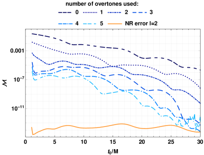
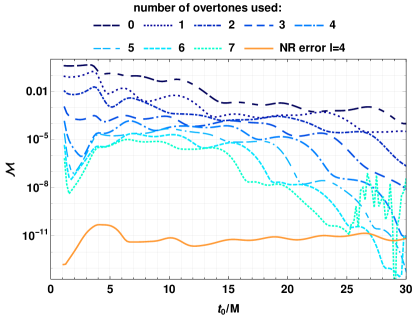
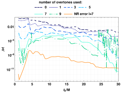
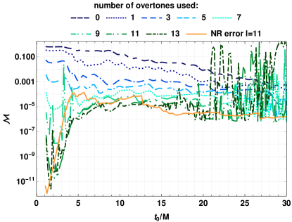
Figure 9: Mismatch between a sample of the NR outer horizon shear modes (upper left panel: $l=2$; upper right: $l=4$; lower left: $l=7$; lower right: $l=11$) and the sum-of-QNM-tones model of Eq. ((23)) at the best-fit parameter values, for a variable number of overtones $n_{\mathrm{max}}$ and as a function of the fit starting time $t_{0}$. An estimate of the numerical uncertainty as a function of $t_{0}$ is also provided (orange continuous line; see Sec. IV.2.1). For the lower two panels, for the sake of readability we have only included the models with the fundamental mode only ($n_{\mathrm{max}}=0$) or with odd numbers of overtones. Mismatch curves with even numbers of overtones remain consistent with the overall trend of decreasing $\mathcal{M}$ with increasing $n_{\mathrm{max}}$ and typically lie in between the curves corresponding to the adjacent odd numbers.

For $n_{\mathrm{max}}=0$ we find again that the fundamental QNM alone matches the shear modes better and better towards later times, but also that for a given $t_{0}$, the quality of the fit provided by this fundamental mode alone overall degrades for increasing $l$. Both of these trends still hold for models additionally including a small number (e.g., $n_{\mathrm{max}}=1$ or $2$) of QNM overtones.

Furthermore, we observe that the quality of the fit clearly improves for almost any $t_{0}$ as the number of overtones is increased. For $l=2$ and $l=4$ here, one can notice a relatively sharp decrease of the mismatch at small $t_{0}$ to small values $\mathcal{M}<10^{-5}$ for a certain number $n_{\mathrm{max}}$ of overtones, beyond which adding more overtones decreases the mismatch less significantly. This occurs at $n_{\mathrm{max}}=3$ for $l=2$ and around $n_{\mathrm{max}}=4$ for $l=4$. This suggests that these numbers of QNM overtones provide a good modeling of the entire dataset for these modes, at least beyond the first $0.5M$ or so after $t_{\mathrm{bifurcate}}$. Such a trend does not appear as clearly for the higher $l$ values shown here, but the mismatch still gets down to small values at early $t_{0}$ for a sufficiently large number of overtones. The number of overtones needed for the mismatch to stay below a certain threshold appears to increase with $l$. For large $l$, the numerical error becomes too large for reliable constraints on large numbers of overtones, and for estimating the number of overtones needed for the mismatch to stay below a too small threshold. For $l=11$ for instance, the mismatch with the $\mathrm{res}=180$ results reaches $\mathcal{M}\simeq 10^{-4}$ for certain values of $t_{0}$, and it appears that any improvement in the mismatch by increasing the number of overtones beyond $n_{\mathrm{max}}=6$ lies within this numerical uncertainty.

While a useful synthetic quantitative tool, the mismatch is based on absolute deviations between the data and the model, and for this reason it does not necessarily clearly reflect how well the damped behavior of the modes is represented by the model at all times. For such damped data, it will more accurately measure the relative deviations to the model towards the early parts of the time interval considered.

For this reason, we also directly examine, for each shear mode $\sigma_{l}$ with $2\leq l\leq 12$, the best-fit multiple-tone QNM models as arising from Eq. ((23)), and we compare them to the corresponding NR data, as the number of included overtones increases. A fixed value of $t_{0}$ shortly after $t_{\mathrm{bifurcate}}$ is used in the fitting process. We show in Fig. 10 on a logarithmic scale the NR $l=2$ shear mode and the best-fit models for several successive $n_{\mathrm{max}}$ values. Two additional examples are similarly presented in Figs. 11 and 12, corresponding to the $l=5$ and $l=10$ modes respectively. Numbers of overtones lower than those shown never provide a relevant match to the shear modes beyond a very short time range past $t_{0}$. Conversely, higher numbers of overtones than those shown provide no visible improvement.

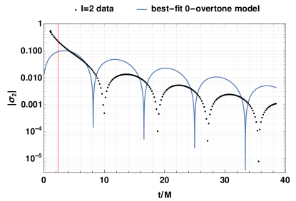
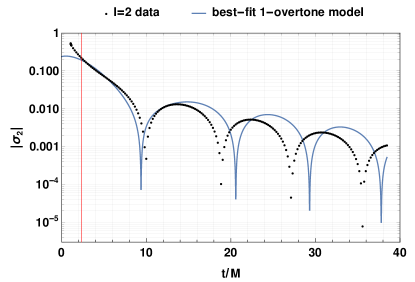
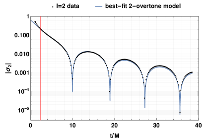
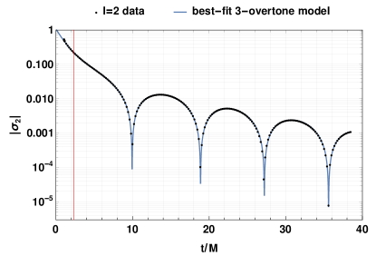
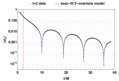
Figure 10: Direct comparison, as a function of the simulation time $t$, of the NR $l=2$ shear mode (black dots) and the associated best-fit models of the class ((23)) (blue continuous lines) including, from left to right and top to bottom, $n_{\mathrm{max}}=0$ to $n_{\mathrm{max}}=5$ overtones. The entire NR dataset is shown, i.e., from $t=t_{\mathrm{bifurcate}}$ to $t=t_{f}$. All of the fits shown in this figure were obtained using the same fit starting time value $t_{0}\simeq 2.3M$. The corresponding $\{t=t_{0}\}$ vertical line, indicating which part of the dataset (to the right of this line) was actually used to constrain the model, is indicated in red on each plot. One can note the good agreement of the model to the data both after and before this starting time for $n_{\mathrm{max}}\geq 3$.

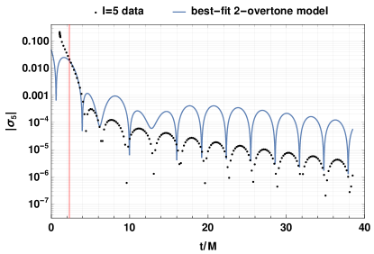
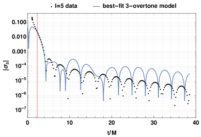
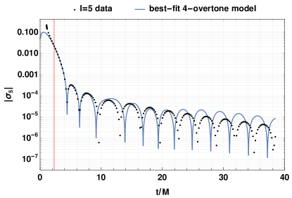
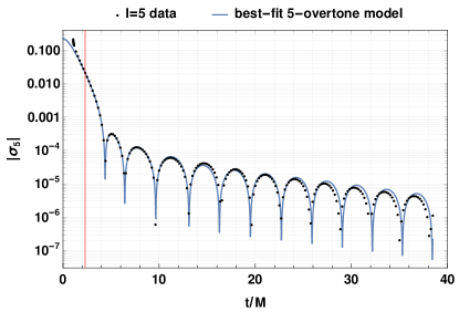
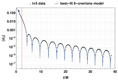
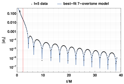
Figure 11: Same as Fig. 10 for the $l=5$ shear mode and $n_{\mathrm{max}}=2$ to $n_{\mathrm{max}}=7$ overtones. The same fit starting time is used. A relatively good agreement to the data is obtained both after and before the fit starting time at $n_{\mathrm{max}}=6$, and this is further improved at $n_{\mathrm{max}}=7$.

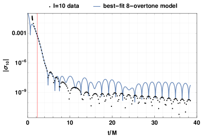
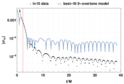
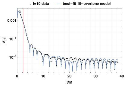
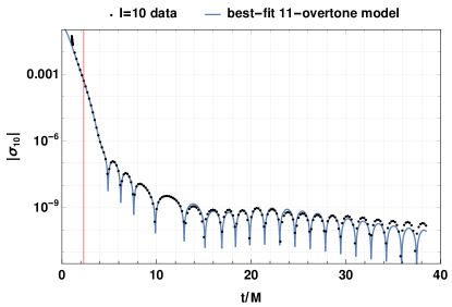
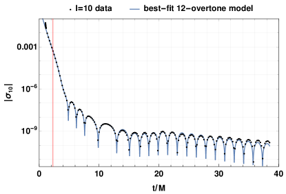
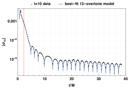
Figure 12: Same as Fig. 10 for the $l=10$ shear mode and $n_{\mathrm{max}}=8$ to $13$ overtones. The same fit starting time is used. A good qualitative agreement to most of the data, including before the fit starting time, is obtained for $n_{\mathrm{max}}=11$ and improves further at late times for $n_{\mathrm{max}}=12$ and $13$, although an oscillating behavior —atypically— reappears in the best-fit model at very early times for $n_{\mathrm{max}}=13$.

For this analysis we have selected a fit starting time $t_{0}=(3/1.3)\,M\simeq 2.3M$. We thus start fitting the data fully within the early decay regime, but not immediately at the formation time $t_{\mathrm{bifurcate}}\simeq 1.06M$. This avoids the times immediately after $t_{\mathrm{bifurcate}}$, up to $t\simeq 1.3M$, where an even steeper decrease is observed due to the infinite slope occurring at the bifurcation with the inner horizon (see Sec. V.1 and Fig. 16). The choice of $t_{0}$ yet about $1M$ further beyond this very specific regime also allows us to evaluate the robustness of the fit results, by checking for the continued agreement to the data at times preceding $t_{0}$.

In overall agreement with the mismatch investigations above, we find that the behavior of each of the shear modes $2\leq l\leq 12$ is well described, over the broad time range $[t_{0},t_{f}]$ considered, by a combination of a sufficiently large number of QNM overtones. For the $l=2$ mode, a combination of two overtones captures well the damping and oscillation features of the mode at all times, and three overtones are enough to ensure a very small relative deviation at all times even including the times $t<t_{0}$. The same remarks hold for $n_{\mathrm{max}}=5$ and $n_{\mathrm{max}}=6$ overtones for $l=5$, while a good modeling of the $l=10$ mode requires $n_{\mathrm{max}}=11$ to $n_{\mathrm{max}}=13$ overtones (with a larger discrepancy to the data at $t<t_{0}$ for $n_{\mathrm{max}}=13$ in this case). Similar results are found for all modes for adequate values of $n_{\mathrm{max}}$.

As suggested by the above examples, the number of overtones required for an accurate representation of the shear modes increases with $l$, reaching large values of $n_{\mathrm{max}}>10$ overtones for $l\geq 10$. In general, a reliable modeling of the mode $l$ typically requires $n_{\mathrm{max}}=l$ or $n_{\mathrm{max}}=l+1$ overtones, occasionally up to $n_{\mathrm{max}}=l+3$ (in particular for the “atypical” cases $l=7$ and $l=10$). These estimates may be unreliable for $l\geq 10$ as the numerical uncertainty may become larger than the contribution of some of the highest overtones considered over most of the time range. In the mismatch analysis above, we pointed out that the improvements of the mismatch to the $l=11$ mode while adding more overtones beyond $n_{\mathrm{max}}=6$ are within our estimate of the numerical error. From a similar consideration, for the example of the $l=10$ mode shown here, the models with $n_{\mathrm{max}}\geq 10$ overtones may actually be poorly constrained for this value of $t_{0}$ due to the uncertainties in the NR results.

Nevertheless, it is quite remarkable that the late-time damped oscillations, the intermediate-time regime and the early steep decay without oscillations of each of the shear modes can be consistently captured by a sum of QNM tones, with a relatively small number of overtones for small $l$. As the real frequencies of the first few modes typically remain close to that of the fundamental mode and thus close to the frequency of the observed late-time oscillations, one would in particular expect such a sum of QNMs to feature oscillations and zeros over the range where the shear modes undergo a steep decay. Instead, the observed oscillation-free early-time regime is well reflected by the best-fit QNM model for large enough $n_{\mathrm{max}}$, including (in nearly all cases) the domain $t<t_{0}$ which is not involved in the fitting procedure.

IV.2.2 Multipole moments

We can repeat the above analysis for the mass multipoles for $2\leq l\leq 12$ (still using the spin-weight-$2$ QNM frequencies). The results are qualitatively very similar to those obtained for the shear modes. Fig. 13 shows the mismatch between each of two example multipoles, $I_{2}$ (left panel) and $I_{7}$ (right panel), and the corresponding best-fit models of the class described by Eq. ((23)), as $n_{\mathrm{max}}$ and $t_{0}$ are varied. The numerical error is estimated in the same way as for the shear in Sec. IV.2.1 above, and is again shown as an orange continuous line. We find again a decrease of $\mathcal{M}$ as $t_{0}$ increases towards $t_{f}$ at fixed $n_{\mathrm{max}}$ at least for $n_{\mathrm{max}}\leq 2$, and also a decrease in mismatch with increasing number of overtones at fixed $t_{0}$. We note that in this case the sharp decrease in mismatch at early $t_{0}$ with increasing number of overtones, for $l=2$, already occurs at two overtones (vs. three overtones for the shear $l=2$ mode). We also generally find again larger mismatches for larger $l$, for a given number of overtones and a given $t_{0}$.

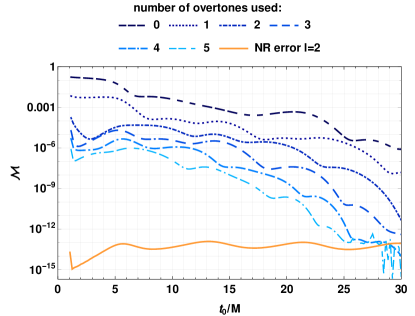
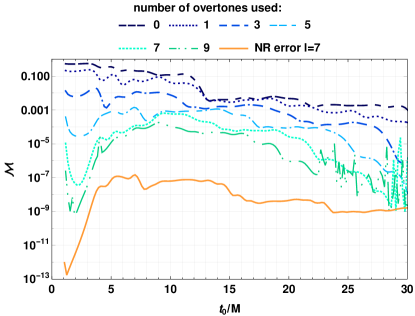
Figure 13: Similar to Fig. 9 for the $l=2$ (left) and $l=7$ (right) mass multipoles as examples. For $l=7$ we again drop the curves obtained for (nonzero) even numbers of overtones for readability. As for the $l=7$ and $l=11$ shear modes in Fig. 9, the missing curves are in line with the overall mismatch decrease trend with increasing $n_{\mathrm{max}}$ observed in the curves shown and can be extrapolated from them.

We then directly compare the best-fit models to the NR multipole results for a fixed fit starting time $t_{0}$ as $n_{\mathrm{max}}$ increases. We use again the same value of $t_{0}\simeq 2.3M$ as for the similar direct comparisons made for the shear modes above in Sec. IV.2.1. Two examples of such comparisons for the multipoles are shown on a logarithmic scale in Fig. 14 ($I_{2}$) and in Fig. 15 ($I_{4}$) for the relevant numbers of overtones. Consistently with the mismatch results for $l=2$, $I_{2}$ shows a small qualitative difference with the results obtained for $\sigma_{2}$. Namely, a two-overtone model already ensures a very small relative deviation to the NR $I_{2}$ data at all times, while a comparable accuracy required three overtones for $\sigma_{2}$. For $I_{4}$, on the other hand, a comparable match is not reached under $n_{\mathrm{max}}=6$, and the best-fit seven-overtone model atypically features an oscillation within the range $[t_{\mathrm{bifurcate}},t_{0}[$. We note that this multipole has a lower magnitude at early times than the surrounding ones $I_{2}$ to $I_{6}$ (see Fig.1, bottom panel), which may be related to this lower fit quality compared to the other modes.

More generally, as for the shear, good matches to the behavior of each multipole $I_{l}$ are obtained over the whole time domain, when including at least $n_{\mathrm{max}}=l$ or $n_{\mathrm{max}}=l+1$ overtones (or occasionally slightly more, such as for $l=4$). In most cases, such a good match also extends back to $t<t_{0}$. Note that for the multipoles, the models with $n_{\mathrm{max}}\geq l$ overtones may be poorly constrained (due to numerical uncertainty) for $l\geq 9$.

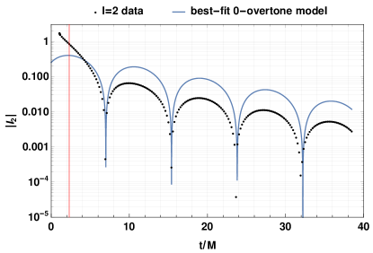
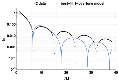
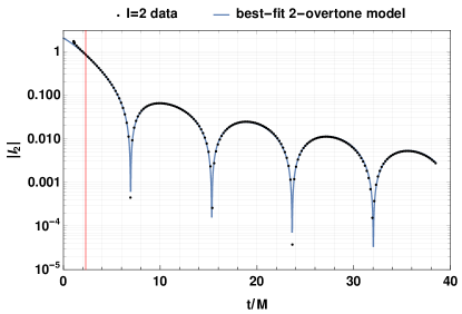
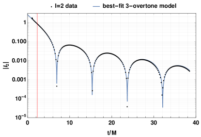
Figure 14: Same as Fig. 10 for the $l=2$ multipole, for $n_{\mathrm{max}}=0$ to $n_{\mathrm{max}}=3$ overtones. We use again the same fit starting time as for the shear modes, $t_{0}\simeq 2.3M$. The model matches well the data both after and before this time at $n_{\mathrm{max}}=2$, and this improves further (especially at $t<t_{0}$) at $n_{\mathrm{max}}=3$.

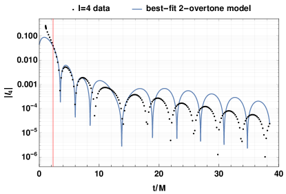
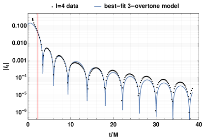
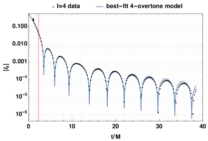
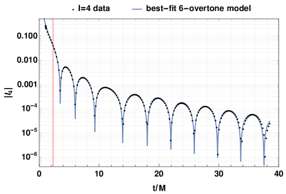
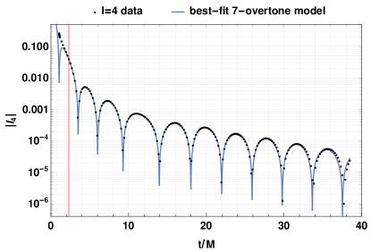
Figure 15: Same as Figs. 10 and 14 for the $l=4$ multipole, for $n_{\mathrm{max}}=2$ to $n_{\mathrm{max}}=7$ overtones. The same fit starting time $t_{0}$ is used. A relatively good agreement to the data is found after and before this time for $n_{\mathrm{max}}=4$, improving for increasing $n_{\mathrm{max}}$, with the exception of $n_{\mathrm{max}}=7$ where the best-fit model displays an unusual behavior for $t<t_{0}$.

V Is the early horizon dynamics really due to overtones?

V.1 General considerations

In the previous section we found, rather surprisingly, that the first few shear modes and multipoles could be well described by a combination of QNMs including the fundamental mode and a few overtones, over the whole time interval available — or at least ignoring the first $\sim 0.3M$ immediately after horizon formation. This conclusion also holds for the larger values of $l$ considered (i.e., at least up to $l=12$), although larger numbers of overtones are needed as $l$ increases. In this section, we consider various criteria, described below, in order to assess the robustness and physical relevance of such a QNM combination description. We shall see, however, that a clear answer remains elusive.

In section IV.1 we confirmed that each of the shear modes and multipoles appears to be fully described asymptotically by the corresponding spin-weight-$2$ fundamental QNM alone for $t\rightarrow\infty$. We however observed deviations from this at intermediate times (e.g., around $t=t_{r}\simeq 15.4M$). We noted that a detectable residual presence of rapidly decaying QNM overtones could be expected in this regime, assuming that the nonlinear deviations to equilibrium are already negligible at these times Bhagwat et al. (2018); Pook-Kolb et al. (2020c). At earlier times $t\lesssim 8M$ however, the area of the outer common horizon is still varying steeply (see Fig. 3), suggesting a still dynamical regime for the horizon at those times. Accordingly, one might not expect the QNMs of the final Schwarzschild black hole to account well for the evolution of the shear flux and geometry of the common horizon from almost immediately after its formation.

In particular, at the time $t_{\mathrm{bifurcate}}$ of the common horizon formation, the observables on this horizon, such as the shear modes and multipoles, have an infinite slope as a function of our time coordinate $t$. This is not a numerical artifact but rather a direct consequence of the bifurcation of the inner and outer common horizons at their joint formation. This is illustrated in Fig. 16 by considering the shear modes on both of the common horizons near their formation and bifurcation time $t_{\mathrm{bifurcate}}$. As a consequence of this infinite slope, no finite sum of QNMs (or any damped sinusoids) can strictly match qualitatively the outer horizon shear modes or multipoles as a function of $t$ for $t\simeq t_{\mathrm{bifurcate}}$. This might however only be due to a coordinate singularity on the horizon. The simulation time $t$ which we use is a time coordinate adapted to our spacetime slicing, and such an infinite slope should indeed occur for any choice of slicing by Cauchy surfaces equipped with an adapted time coordinate. On the other hand, this coordinate is not suitable around $t\simeq t_{\mathrm{bifurcate}}$ for the description of the smooth $3$-surface formed by the union of both common horizons. One could imagine using instead, for example, the radius of the horizon as a more adapted coordinate for this purpose. This will be discussed elsewhere. In this work we shall be content with using the simulation time $t$, discarding a short time range of about $0.3M$ after $t_{\mathrm{bifurcate}}$ from our analyses. This range corresponds to a short faster-than-exponential decrease that can be observed in the shear modes and multipoles and that matches the vertical tangent at $t=t_{\mathrm{bifurcate}}$. We have seen that the shear modes and multipoles can be well described by combinations of QNM tones at all times past this short regime.

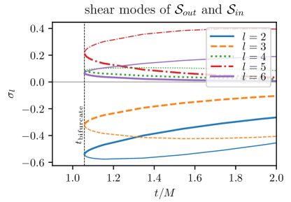
Figure 16: Numerically computed first six shear modes as a function of the simulation time $t$ on the outer common horizon $\mathcal{S}_{out}$ (thicker lines) and on the inner common horizon $\mathcal{S}_{in}$ (thinner lines), near the formation/bifurcation time $t=t_{\mathrm{bifurcate}}$ (highlighted as a vertical dashed line). The continuity of these variables across both horizons and the resulting vertical tangent at bifurcation are easily visible. The higher shear modes, and the multipoles, have the same behavior.

In the present section, we thus aim at investigating whether the results we presented in section IV should really be interpreted as the physical presence of initially high-amplitude QNM overtones determining the entire evolution of the outer common horizon past the first $\sim 0.3M$. We must also consider the alternative — that these results are simply an artifact of fitting the observables $\sigma_{l}$ and $I_{l}$ with damped sinusoids with sufficiently many free parameters.

We note in particular that the modes at large $l$ can only be well matched by a sum of QNM tones if this sum extends to a large number $n_{\mathrm{max}}$ of overtones, leaving a large number of degrees of freedom for fitting the data (that is, $2n_{\mathrm{max}}+2$ degrees of freedom; with the minimum $n_{\mathrm{max}}$ required ranging from $10$ to $14$ for $10\leq l\leq 12$). The numerically computed shear modes and multipoles feature a steeper and steeper early-time ($t_{\mathrm{birfurcate}}+0.3M\lesssim t\lesssim t_{\mathrm{birfurcate}}+3M$) damping as $l$ increases. On the other hand, the damping rates of the QNMs for a given $n$ are independent of $l$ to first approximation, but increase with $n$ (see, e.g., Sec. 3.1 of Kokkotas and Schmidt (1999); an illustration of this can also be seen in Table 1 of the present work, right panel). It was thus expected from the observed behavior of the shear modes and multipoles that their modeling in terms of QNMs would require higher overtones for larger $l$. It is not obvious however from a theoretical perspective that a larger early-time amplitude of high overtones should have been expected a priori for higher shear modes or multipoles.

One may come back to the generalized model of Eq. (III.1) with multiple tones ($n_{\mathrm{max}}\geq 1$), leaving the parameters $\alpha_{l0n}$ and $\beta_{l0n}$ free, and attempt to check if the best-fit model indeed recovers the QNM frequency values, corresponding to $\alpha_{l0n}=\beta_{l0n}=0$. Unfortunately, already for $n_{\mathrm{max}}=1$ and even more for larger $n_{\mathrm{max}}$, the frequency deviation parameters appear to be very hard to constrain — even when the rescaling procedure of Eq. ((21)) is applied. These parameters typically feature large fitting uncertainties and overlaps between tones or with zero-frequency models ($\alpha_{l0n}=-1$). This is likely due to the small differences between the QNM real frequencies (used as reference values) for successive tones, as well as to the rapid decay of QNM overtones. Accordingly we cannot really conclude on the actual presence of QNM overtones from such an analysis. This does however suggest that constraining the deviations of the complex frequencies of a combination of damped sinusoids from the theoretical QNM frequency values can be very challenging in general, even for zero-noise, low-systematic error data.

In the following subsections we will thus rather probe the robustness of the QNM modelling using several tests of fit stability and fit comparison. These tests provide more insight than the approach mentioned hereabove, even though they still do not allow us to reach a definitive conclusion. We will simply focus on the shear for this investigation, and specifically on the $l=2$ shear mode as an example and as an easy case that can be modeled with a relatively small number of overtones.

V.2 Comparing models with different numbers of overtones but an equal number of free parameters

We first consider the relative quality of the fits provided either by a sum of a few QNM tones, or by another model of the general class of Eq. (III.1) with less modes but some of the parameters $\alpha_{l0n}$ and $\beta_{l0n}$ left free rather than being set to zero. We choose the second model in such a way that both models have the same number of free parameters. We will consider two such pairs of models, with respectively four and six free parameters. We compare the models within each pair in terms of their mismatch to the NR $l=2$ shear mode for the best-fit parameters (without applying a rescaling such as that of Eq. ((21))), as a function of the fit starting time $t_{0}$.

Fig. 17 shows this mismatch for the $(n_{\mathrm{max}}=1)$-overtone model of the class of Eq. ((23)) (green continuous line), where all frequencies are set to the QNM values; and for the single-mode model with free frequencies used in section IV.1 and given by Eq. ((22)) (red dashed line). The free parameters are $\{A_{0},\phi_{0},A_{1},\phi_{1}\}$ in the first case and $\{A_{0},\phi_{0},\alpha_{0},\beta_{0}\}$ in the second case. These results suggest a small preference at nearly all times for the one-overtone model with QNM frequencies over a single-damped-sinusoid model even though the complex frequency of the latter is freely adjusted. The improvement in mismatch does however occur at most but not all values of $t_{0}$, and barely goes beyond $1$ order of magnitude when it occurs. In particular, for most values of $t_{0}/M\gtrsim 28$, i.e. at very late times, we obtain similar values of the mismatch $\mathcal{M}$ for both models considered. This is consistent with Fig. 7 since, in this regime, deviations to a fundamental-mode-only model (with QNM complex frequency) are expected to be mostly negligible.

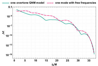
Figure 17: Comparison of the respective mismatches to the NR shear $l=2$ mode for two four-parameter models (see Sec. V.2 for details), as a function of the fit starting time $t_{0}$.

Fig. 18 shows the similar mismatch for two six-parameter models. Both models assume the presence of the fundamental QNM, which we seem to recover asymptotically at late times. They both consider an additional contribution, which takes the form of either the first two QNM overtones, or of a single damped sinusoid with unconstrained complex frequency. The first model (green continuous line) thus corresponds to the $(n_{\mathrm{max}}=2)$-overtone model with QNM frequencies of the class of Eq. ((23)), with free parameters $\{A_{0},\phi_{0},A_{1},\phi_{1},A_{2},\phi_{2}\}$. The second model (red dashed line) corresponds to the general ansatz of Eq. (III.1) for $n_{\mathrm{max}}=1$ and with $\alpha_{l00}$ and $\beta_{l00}$ set to zero. The free parameters in this case are $\{A_{l00},\phi_{l00},A_{l01},\phi_{l01},\alpha_{l01},\beta_{l01}\}$. No clear preference is found for either model, both of them alternately having the lowest mismatch for various ranges of $t_{0}$, and with very small differences between both mismatch values.

Hence, a {fundamental QNM + first QNM overtone} model is only marginally preferred to a single-damped-sinusoid model, and assuming the presence of the fundamental QNM, we cannot conclude about the additional presence of two QNM overtones vs. that of an arbitrary single additional damped sinusoid. This neither confirms nor rules out the actual presence of QNM overtones, but hints again quite strongly at the difficulty of confidently determining a) the presence of overtones and b) the frequencies of multiple damped sinusoids that may be present in the data.

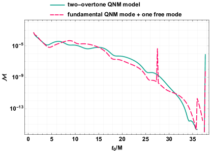
Figure 18: Comparison of the respective mismatches to the NR shear $l=2$ mode for two six-parameter models (see Sec. V.2 for details), as a function of the fit starting time $t_{0}$.

V.3 Comparison to a toy model with altered real frequencies

We now investigate how the quality of multiple-tone fits depends on deviations in the frequencies of the tones with respect to the QNM values. We here focus on the real frequencies, noting that the imaginary frequencies (or damping rates) of successive QNM tones $n$ are well separated, while the corresponding real frequencies vary by smaller amounts for small $n$ values (Sec. 3.1 of kokkotas:1999bd; see also Table 1 hereabove). For the $(l=2,\,m=0)$ mode considered here, the real frequencies of the first three QNM overtones $\omega_{20n},n=1,2,3$, for instance, are smaller than the fundamental-mode one $\omega_{200}$ by about $7\%$, $19\%$ and $33\%$ respectively (see Table 1, left panel).

For this purpose, we consider a family of arbitrary toy models following the general ansatz of Eq. (III.1), with a variable total number of overtones $n_{\mathrm{max}}$. We define this family by setting $\alpha_{l00}$ and all the $\beta_{l0n}$ parameters to zero, i.e., we keep the fundamental QNM and we keep all damping rates at the QNM values, and by setting the other $\alpha_{l0n}$ parameters, $n>0$, to a specific choice of nonzero values. Our choice here is to set every $\alpha_{l0n}$ such that the real frequency of each tone in the model stays equal to the fundamental QNM real frequency: $\omega_{l0n}(1+\alpha_{l0n})=\omega_{l00}\,\forall n$. We thus end up with the following family of models, parametrized by $n_{\mathrm{max}}$:

$$X_{l}=\sum_{n=0}^{n_{\mathrm{max}}}A_{l0n}\,\exp\left[-\frac{t-t_{r}}{\tau_{l0n}}\right]\,\cos\left[\omega_{l00}\,(t-t_{r})+\phi_{l0n}\right]\;.$$ ((24))

The free parameters of the models are the amplitudes $A_{l0n}$ and the phases $\phi_{l0n}$. We probe the ability of these artificial models to match the shear $l=2$ mode at all times as $n_{\mathrm{max}}$ is varied, in a similar way as was done, e.g., for Fig. 10 in section IV.2.1. That is, we set the same early fit starting time $t_{0}\sim 2.3M$ as for the latter figure and we directly study the relative deviation of the best-fit model to the NR data (and to its general behavior) for each $n_{\mathrm{max}}$, without using a rescaling such as that of Eq. ((21)) in the fitting process.

Fig. 19 shows the results similarly to Fig. 10 with the best-fit model for each $n_{\mathrm{max}}$ as a continuous line and the NR data as dots, as a function of $t$ and on a logarithmic scale. We show here only the most relevant values of $n_{\mathrm{max}}=2$ and $n_{\mathrm{max}}=3$. $n_{\mathrm{max}}=0$ (fundamental QNM only, already considered earlier) and $n_{\mathrm{max}}=1$, do not provide a good match to the overall behavior of the shear mode, while values of $n_{\mathrm{max}}>3$ show little visible difference to the $n_{\mathrm{max}}=3$ case.

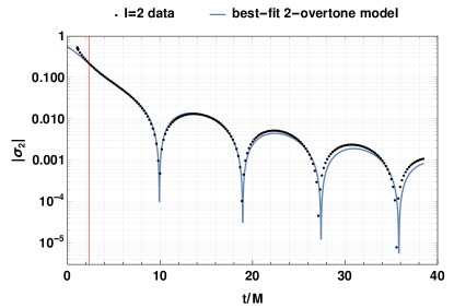
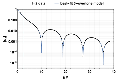
Figure 19: Direct comparison of the NR $l=2$ shear mode (black dots) and the associated best-fit toy models as introduced in section V.3 (blue continuous lines; see this section for details), as a function of the simulation time $t$. We show here the results for the most relevant numbers of $n_{\mathrm{max}}=2$ (left panel) and $n_{\mathrm{max}}=3$ (right panel) additional modes beyond the fundamental QNM. The vertical red line on each panel indicates the $\{t=t_{0}\}$ line, where the starting time $t_{0}$ used for the fits is set to a constant value given by $t_{0}/M=3/1.3\simeq 2.3$, as for the similar analyses with a different model presented in section IV.2. For a given $n_{\mathrm{max}}$, the agreement of the best-fit toy model to the NR data is comparable to that obtained with the actual QNM model in Fig. 10, both after and before $t_{0}$.

Interestingly, we find again for this artificial model a rather good match to the data for $n_{\mathrm{max}}=2$, and a very good match at all times (including prior to $t_{0}$ but after $t\simeq t_{\mathrm{bifurcate}}+0.3M$) for $n_{\mathrm{max}}=3$. The results are qualitatively very similar to those obtained with the multiple-QNM-tones model of Eq. ((23)) in section IV.2, despite the unphysical real frequency values used here for the overtones. Hence, our conclusions of a good modeling of the shear modes or multipoles by combinations of sufficiently many QNM tones are not very sensitive to the actual frequencies (at least regarding the real part) used in the overtones model. We see here that similar conclusions can be reached with models that do not match the GR QNM values for $n>0$.

V.4 Stability of the multiple-QNM fits with the fit time range

We finally study some aspects of the stability of the best-fit parameters when fitting the multiple-tone QNM model of Eq. ((23)) to the NR data over the range $[t_{0},t_{f}]$ as $t_{0}$ is varied. Such a stability can be seen as a necessary condition for the consistent presence of a set of QNM overtones in the data. If these modes are present, then for instance their amplitudes should be recovered consistently over a range of $t_{0}$ values where they are detectable.

We have already mentioned some stability properties of the fits provided by this model for large enough numbers of overtones in section IV.2. It is indeed noteworthy that when selecting a fit starting time $t_{0}\simeq 2.3M\simeq t_{\mathrm{bifurcate}}+1.2M$, in almost all cases where any given shear mode or multipole is well matched by the model after $t_{0}$, the nonoscillating damped regime extending before $t_{0}$ to $t\simeq t_{\mathrm{bifurcate}}+0.3M$ is also well recovered, qualitatively and quantitatively. These QNM models thus consistently match the behavior of the data even at times where they have not been constrained. This suggests that the corresponding QNM overtones are recovered consistently for some range of times around this $t_{0}$.

Here we turn to the investigation of the best-fit amplitude parameters $A_{n}$ obtained for each tone $n$ in multiple-tone models of the class of Eq. ((23)) (hence, with all frequencies equal to the QNM values), still for the example of the shear $l=2$ mode. These parameters are by definition amplitudes computed at the fixed time $t_{r}$, and we check for their constancy as we vary the time $t_{0}$ at which the fit is started. The same or a similar test has been used to check for the presence of overtones in numerical gravitational-wave ringdown models e.g. in Bhagwat et al. (2020); Giesler et al. (2019); Cook (2020).

As we want to retrieve the amplitudes of the tones, we here apply the rescaling procedure given by Eq. ((21)) prior to fitting. Note that we still expect the amplitudes (at $t_{r}$) of the overtones not to be accurately determined for too large $t_{0}$, as the overtones are damped much faster than the fundamental mode and hence still decay in the rescaled data.

We focus first on the model in the case of $n_{\mathrm{max}}=3$, which we found to be the smallest number of overtones matching very well the behavior of $\sigma_{2}$ at all times. Fig. 20 shows the resulting best-fit amplitude parameters for the fundamental mode and for the three overtones considered, as functions of $t_{0}$, along with their $1\sigma$ fitting uncertainties (Eq. ((18))).

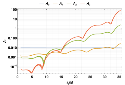
Figure 20: Best-fit amplitudes at $t_{r}$ (with $1\sigma$ uncertainties as given by Eq. ((18))) as a function of the fit starting time $t_{0}$ for the fundamental mode and overtones in the ($n_{\mathrm{max}}=3$)-overtone QNM model of Eq. ((23)), for the shear $l=2$ mode. The rescaling procedure given by Eq. ((21)) has been used before fitting.

The amplitude parameter $A_{0}$ of the fundamental mode is remarkably constant throughout the figure, providing strong further support for the presence of this mode in the data. The amplitude parameters $A_{n}$ ($n>0$) of the overtones, on the other hand, are clearly inconsistent between different values of $t_{0}\gtrsim 4M$. This does not really contradict the presence of overtones in the data as these amplitudes are expected to be poorly determined beyond early times once the overtones have decayed. Interestingly however, all overtones have a stable best-fit amplitude parameter over the range $1.5M\lesssim t_{0}/M\lesssim 4M$, which corresponds to the regime of early-time exponential decay. Each of the amplitudes is thus consistently determined over multiple values of $t_{0}$ if this regime is accounted for in the fit. We note that the ratios of the overtone amplitudes computed at the horizon formation, $A_{n}\exp[(t_{r}-t_{\mathrm{bifurcate}})/\tau_{l0n}]$ ($n>0$), to the amplitude of the fundamental mode at the same time $A_{0}\exp[(t_{r}-t_{\mathrm{bifurcate}})/\tau_{l00}]$, as determined here from the stable early-time best-fit values of $A_{n}$ and $A_{0}$, are of the order of $\sim 2$, $\sim 23$ and $\sim 34$ for $n=1$, $n=2$ and $n=3$ respectively.

We show for comparison in Fig. 21 the best-fit amplitude parameters obtained in the same way with instead $n_{\mathrm{max}}=4$ overtones included in the model. The resulting $A_{0}$ is still constant over the whole time range considered and $A_{1}$ is still relatively stable over the same early-time interval as above, with values roughly consistent with those obtained from the three-overtone model. The higher overtones ($n\geq 2$) on the other hand do not appear to be stable over any time range. This may however simply indicate that their amplitudes cannot be constrained accurately enough even in the exponential damping regime due to a large number of free parameters and a too quickly decaying fourth overtone. For $\sigma_{2}$, $n_{\mathrm{max}}=3$ seems to be an optimal number of overtones that models well the data at all times while still allowing the amplitude of each tone to be correctly constrained.

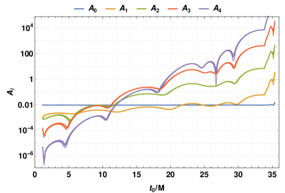
Figure 21: Same as Fig. 20, for the $(n_{\mathrm{max}}=4$)-overtone model of Eq. ((23)).

The considerations of this subsection — including the discussion recalled hereabove from section IV.2 — still do not provide any definitive conclusion about the actual presence of QNM overtones in the shear modes or multipoles, in particular since the stability of the best-fit model over some time range is a necessary, but not a sufficient condition for their presence. Yet these results perhaps represent the most supportive clue that we obtain in favor of the behavior of the horizon being indeed dominated by QNMs from shortly after its formation. The results of the previous subsections would not directly contradict such a statement. They would rather point towards the difficulty of separating QNM overtones from any other combination of damped sinusoids with roughly comparable complex frequencies (and thus of deciding on the presence of QNM overtones vs. such other decaying modes), and even of determining how many tones would have non-negligible contributions.

VI Conclusion and discussion

We have shown in this paper that the dynamics of the final apparent horizon in a binary black hole merger can be very well described by the quasinormal modes of the final black hole, from shortly after this horizon is formed onward. We have studied two quantities of interest, namely the shear of the outgoing normal at the horizon, and the horizon multipole moments; both of these are well modeled by quasinormal modes provided a large enough number of overtones is included. We have considered here a high-precision numerical simulation of a head-on collision of nonspinning black holes, but we expect these results to qualitatively hold for other configurations (of higher astrophysical interest) as well.

We have first confirmed that the behavior of each of the shear modes $\sigma_{l}$ and of the horizon mass multipole moments $I_{l}$, for $2\leq l\leq 12$, is dominated at late times by the corresponding fundamental quasinormal mode. This is compatible with linear perturbation theory, which can be expected to hold in this regime and predicts an asymptotic predominance of the fundamental quasinormal modes since the associated overtones have shorter damping times. This result strengthens the conclusions of Pook-Kolb et al. (2020c), and supports the presence of correlations between the emitted gravitational waves and the dynamics of the final black hole horizon (cf. Prasad et al. (2020)). Deviations from a description only in terms of the fundamental mode are however also evident, especially at early and intermediate times. This is accounted for by also including the higher overtones. We have shown that the shear and multipole moments, for essentially the entire time after the common horizon formation, are well described by superpositions of quasinormal modes including the overtones.

These results are in qualitative agreement with studies of the gravitational waveform extracted far away from the source. For example, in Giesler et al. (2019) it is found that the dominant $(l=|m|=2)$ harmonic of the gravitational waveform for a particular quasicircular initial configuration (with mass ratio $1.22$ and moderate spins aligned with the orbital angular momentum) is well modeled right up to the peak of the strain by including up to seven overtones. The ability to detect and separate the successive overtones in the early stages of the ringdown, before they have decayed, would improve the prospects for black hole spectroscopy, and for observational probes of the black hole no-hair theorem.

In the present work, we have probed another part of spacetime by focusing on the horizon of the final black hole; we however expect strong correlations between both dynamics, arising from the same source Prasad et al. (2020). The simpler geometry in our study, and the focus on the horizon, allowed for a high numerical precision and for an investigation of all geometric modes up to $l=12$, rather than just the dominant $l=2$ mode, for both the shear and the multipole moments. For all of these modes, we have obtained similar qualitative results. In particular, in the case of the $l=2$ mode, we have found that two to three overtones suffice for an accurate modeling of both variables from shortly after the horizon formation onward. We have however also noticed the general increase in the number of overtones necessary for a good description of the geometric $l$ mode as $l$ increases.

Such results remain surprising because, shortly after the common horizon is formed, it is highly distorted and cannot be described as a linear perturbation of a Schwarzschild horizon. As evidence for this, we have noted that the area of the horizon increases at a very significant rate in this regime. The total relative change in area is only of about $6\%$ however, so it could be argued that perturbation theory is still of some utility. One can then wonder whether obtaining a description of the horizon dynamics in terms of ringdown modes in this regime implies that the horizon is, in some suitable sense still to be understood, still a small perturbation of a stationary black hole. We have accordingly studied, through various possible criteria, whether one should conclude a) at the linear perturbation spectrum indeed already driving the horizon dynamics at early times, or b) at the more prosaic alternative that the quasinormal modes are just a suitable function basis for the shear and the multipoles, so that there is no deeper interpretation of these results.

Despite this investigation, and given the lack of a calculation from first principles, a conclusive answer to this question is still elusive. We have noted that the infinite slope featured by all shear modes and multipoles at $t_{\mathrm{bifurcate}}$ prevents their formal description by a finite sum of QNMs at horizon formation, at least in terms of the $t$ parameter used. Nevertheless, this constraint does not rule out such a model even at only slightly later times such as during the observed “early-time” decay phase at $0.3\lesssim(t-t_{\mathrm{bifurcate}})/M\lesssim 3$. Hypothesis a) is supported by the stability observed to some extent in the best-fit amplitudes of each mode when the time $t_{0}$ at which the fit is started varies and spans the early-time range quoted above. This stability also manifests itself in the continued qualitative agreement of the model to the data at times prior to $t_{0}$ that is typically observed when $t_{0}$ lies in this range. On the other hand, models with lower numbers of overtones but some of the overtone frequencies let free to deviate from the QNM values, did not show a clear preference for the QNM overtones spectrum. The same was found using an example toy model with real frequencies artificially set slightly away from the QNM values. This is compatible with hypothesis b), but these results do not rule out the actual predominance of overtones at early times, hypothesis a), given that a clear preference for non-QNM frequencies was not found either. This rather hints at the difficulty of resolving individual modes in a sum of damped sinusoids with frequencies comparable to that of the QNMs, and of determining how many such modes can be included and constrained, even with essentially noise-free data. We expect these issues —including the overall difficulty of firmly ruling out the predominance of nonlinearities over overtones at early times— to hold similarly when the ringdown is analyzed from the emitted gravitational waves, complicating an overtone-based spectroscopy. The lack of a clear-cut recovery of the QNM overtone frequencies, in particular, was indeed also observed for the dominant $(l=|m|=2)$ gravitational-wave mode during ringdown in a binary black hole merger simulation in Bhagwat et al. (2020).

Turning now to future directions, there are a few straightforward possible extensions of the present work. First, the present analysis may be completed by a closer look at the more involved behavior of the vector modes $\xi_{l}$ (see Fig. 2 and the associated brief discussion in section II.2.3). Within the same setup as considered here, it would also be natural to try other parametrizations of “time” to circumvent the infinite slope at $t_{\mathrm{bifurcate}}$ in each of the observables as functions of $t$. This could also allow for a consistent joint treatment of both the inner and outer common horizons, which constitute indeed a single smooth hypersurface in spacetime. Second, one can look for a possible generalization of the results to a wider variety of configurations, including the astrophysically important quasicircular orbits and accounting for black hole spin. Third, a more fundamental investigation of the mechanisms driving the early-time dynamics of the outer common horizon could shed more light onto the fast exponential decays observed at these times for all of the shear modes and multipoles. We have found here that quasinormal overtones can indeed combine in such a way as to produce this behavior. An investigation of the mechanisms driving it could either provide more insight into why such a combination would take place, or rule out quasinormal modes as a relevant explanation for this (possibly still nonlinear) regime altogether.