Ensemble sampler for infinite-dimensional inverse problems

Abstract

We introduce a new Markov chain Monte Carlo (MCMC) sampler for infinite-dimensional inverse problems. Our new sampler is based on the affine invariant ensemble sampler, which uses interacting walkers to adapt to the covariance structure of the target distribution. We extend this ensemble sampler for the first time to infinite-dimensional function spaces, yielding a highly efficient gradient-free MCMC algorithm. Because our new ensemble sampler does not require gradients or posterior covariance estimates, it is simple to implement and broadly applicable.

1 Introduction

In many Bayesian inverse problems, Markov chain Monte Carlo (MCMC) methods are needed to approximate distributions on infinite-dimensional function spaces, for example in groundwater flow Iglesias_2014 , medical imaging dunlop2016bayesian , and traffic flow coullon2020mcmc . Yet designing efficient MCMC methods for function spaces has proved challenging.

The earliest proposed sampler for function spaces was the preconditioned Crank-Nicolson algorithm (PCN, beskos2008mcmc ). PCN is easy to code and broadly applicable, but it is not always efficient. When sampling from a posterior distribution that is poorly scaled or multimodal, PCN can require a huge number of samples to accurately calculate statistics cotter2013mcmc .

Recent gradient-based MCMC methods cotter2013mcmc ; cui2014likelihood ; beskos2017geometric , preconditioned MCMC methods zhou2017hybrid ; rudolf2018generalization , and SMC methods Kantas2014SMC have improved on the computational efficiency of PCN. However, these new samplers require gradients or posterior covariance estimates that may be challenging to obtain. Calculating gradients is difficult or impossible in many high-dimensional inverse problems involving a numerical integrator with a black-box code base chen2016accelerated . Additionally, accurately estimating posterior covariances can require a lengthy pilot run or adaptation period roberts2009examples . These concerns raise the question: is there a functional sampler that outperforms PCN without requiring gradients or posterior covariance estimates?

To address this question, we turn to the literature on finite-dimensional MCMC. In finite-dimensional spaces, there is a gradient-free sampler that avoids explicit covariance estimation yet adapts naturally to the covariance structure of the sampled distribution. This sampler, called the affine invariant ensemble sampler (AIES, goodman2010ensemble ), is easy to tune, easy to parallelize, and efficient at sampling spaces of moderate dimensionality ($d\leq 20$). AIES is used extensively due to its implementation in the popular emcee package for python foreman2013emcee .

The main contribution of this work is to propose a new functional ensemble sampler (FES) that combines PCN and AIES. To apply this new sampler, we first calculate the Karhunen–Loève (KL) expansion for the Bayesian prior distribution, assumed to be Gaussian and trace-class. Then, we use AIES to sample the posterior distribution on the low-wavenumber KL components and use PCN to sample the posterior distribution on the high-wavenumber KL components. Alternating between AIES and PCN updates, we obtain our functional ensemble sampler that is efficient and easy to use, without requiring detailed knowledge of the target distribution.

In past work, several authors have proposed splitting the Bayesian posterior into low-wavenumber and high-wavenumber components and then applying enhanced sampling to the low-wavenumber components law2014proposals ; Kantas2014SMC ; cui2016dimension ; beskos2017geometric ; beskos2018multilevel . Yet compared to these other samplers, FES is unique in its simplicity and broad applicability. FES does not require any derivatives, and the need for derivative-free samplers has previously been emphasized in chen2016accelerated ; hu2017adaptive ; zhou2017hybrid ; beskos2018multilevel . FES also eliminates the requirement for posterior covariance estimates. Lastly, FES is more efficient than other gradient-free samplers in our tests.

In two numerical examples, we apply FES to challenging inverse problems that involve estimating a functional parameter and one or more scalar parameters. In our first example, we consider the advection equation

$$\begin{cases}\frac{\partial\rho}{\partial t}+c\frac{\partial\rho}{\partial x}=0,&t>0,\\ \rho=\rho_{0},&t=0.\end{cases}$$ (1)

We simultaneously estimate the advection speed $c$ and the initial condition $\rho_{0}$ from a set of noisy observations. We compare the performance of PCN and FES and find that PCN mixes slowly because $c$ and $\rho_{0}$ are highly correlated under the posterior distribution. In comparison, FES mixes more quickly, reducing integrated autocorrelation times sokal1997monte by two orders of magnitude.

In our second example, we consider the Langevin diffusion

$$\begin{cases}\mathop{dX}=P\mathop{dt},&t>0,\\ \mathop{dP}=-\alpha X\mathop{dt}+\sigma\mathop{dW},&t>0,\\ X=P=0,&t=0.\end{cases}$$ (2)

We simultaneously estimate the drift parameter $\alpha$, the diffusion parameter $\sigma$, and the posterior path $\left(X_{t}\right)_{0\leq t\leq 10}$ from noisy observations. We compare the performance of PCN, FES, and an alternative derivative-free sampler zhou2017hybrid that explicitly estimates the posterior covariance matrix. We conclude that FES is the fastest available gradient-free sampler for this challenging, multimodal test problem.

The rest of the paper is organized as follows. Section 2 reviews the PCN and AIES samplers, Section 3 introduces the new ensemble sampler for function spaces, Section 4 presents numerical examples, and Section 5 concludes. Code to reproduce the examples is available on Github.

2 Background on MCMC samplers

In this section, we explain why it is difficult to approximate a Bayesian posterior distribution on an infinite-dimensional function space. Then, we describe the preconditioned Crank-Nicolson sampler (PCN, beskos2008mcmc ) which can be used for this approximation task. Lastly, we describe the affine invariant ensemble sampler (AIES, goodman2010ensemble ), an efficient sampler for finite-dimensional spaces that has not previously been extended to the infinite-dimensional setting.

2.1 Infinite-dimensional inverse problems

In a typical infinite-dimensional Bayesian inverse problem, the goal is estimating a posterior distribution

$$\pi(\mathop{du})\propto\exp\left(\phi(u)\right)\pi_{0}(\mathop{du}),$$ (3)

where $u$ is a square-integrable function on a domain $\Omega\subseteq\mathbb{R}^{d}$, $\phi(u)$ is a log-likelihood functional, and $\pi_{0}=\mathcal{N}(0,C)$ is a Gaussian prior distribution.

To estimate $\pi$, we must select a finite-dimensional approximation space and then sample $\pi$ restricted to this space. However, ensuring high accuracy with this approach is difficult. To accurately calculate statistics of the posterior distribution, a high-dimensional approximation space is needed. Yet, as we increase the dimensionality, the acceptance probability for a standard MCMC sampler, such as the Metropolis random walk sampler metropolis1953equation , sinks to zero. Hence, the MCMC sampler takes an increasingly long time to move anywhere, and sampling from $\pi$ becomes tediously slow cotter2013mcmc .

2.2 Preconditioned Crank-Nicolson

PCN solves the problem of vanishing acceptance probabilities by proposing MCMC moves that are always accepted under the Gaussian prior distribution. Because of this stability property, even as we increase the dimensionality of the approximation space, the average acceptance probability remains bounded away from zero hairer2014spectral .

Starting from a position $U$, the PCN update is

$$\tilde{U}=\sqrt{1-\omega^{2}}U+\omega\xi,$$ (4)

where $\xi\sim\mathcal{N}\left(0,C\right)$ is a random draw from the Gaussian prior and $\omega\in\left(0,1\right]$ is a step size parameter. If $\omega\ll 1$, the proposal is a small perturbation of the position $U$, whereas if $\omega=1$ the proposal is independent from $U$. The main computational cost of PCN then comes from evaluating the acceptance probability

$$\min\left\{1,\exp\left(\phi(\tilde{U})-\phi(U)\right)\right\},$$ (5)

which requires calculating the log-likelihood functional at the proposed parameter value $\tilde{U}$.

PCN is a simple, widely applicable approach that requires little more than making inexpensive proposals and evaluating the log-likelihood at the proposed parameter values. However, the main limitation of PCN is the slow convergence of statistics when the posterior distribution is poorly scaled or multimodal. This slow convergence has led to myriad efforts to improve on PCN’s sampling speed cotter2013mcmc ; cui2014likelihood ; Kantas2014SMC ; beskos2017geometric ; zhou2017hybrid ; rudolf2018generalization , but the available methods require gradients or covariance estimates that can be difficult to obtain.

2.3 Affine invariant ensemble sampler

The affine invariant ensemble sampler (AIES, goodman2010ensemble ) is a finite-dimensional MCMC sampler with the remarkable property of affine invariance. Affine invariance means that the sampler remains completely unchanged if the state space is stretched, compressed, or translated by an affine transformation $x\mapsto Ax+b$. Because of this property, AIES efficiently samples from distributions that are wide in some directions and narrow in other directions. These “poorly scaled” distributions would cause problems for other samplers, but they do not compromise the performance of AIES.

To sample from a density $\pi$ on $\mathbb{R}^{M}$, AIES generates an ensemble of walkers $\overrightarrow{X}=(X_{1},...X_{L})$ that is invariant with respect to the product density $\pi\left(x_{1}\right)\cdots\pi\left(x_{L}\right)$ on $\mathbb{R}^{ML}$. To update the ensemble, AIES proposes sliding one walker toward or away from another walker. Then, AIES accepts or rejects the proposal according to a Metropolis-Hastings step. The proposals and acceptance probabilities are invariant under affine transformations, so the scheme is affine invariant overall.

To perform the AIES proposal step, we randomly choose a walker $X_{i}$ and a second walker $X_{j}\neq X_{i}$. Then, we propose moving the walker $X_{i}$ to the new position

$$\tilde{X}_{i}=X_{i}+\left(1-Z\right)\left(X_{j}-X_{i}\right),$$ (6)

where $Z$ is a random number in an interval $\left[1/a,a\right]$, chosen with density $g\left(Z\right)\propto 1/\sqrt{z}$. Typically, $a=2$ in applications, but more generally $a$ is a parameter that modulates the step size. The main computational cost of AIES then comes from evaluating the acceptance probability

$$\min\left\{1,Z^{M-1}\frac{\pi(\tilde{X}_{i})}{\pi(X_{i})}\right\},$$ (7)

which requires calculating the density $\pi$ at the proposed position $\tilde{X}_{i}$.

AIES is a popular and efficient sampler for low- and moderate-dimensional densities ($M\leq 20$). AIES would not typically be an efficient sampler for higher-dimensional denities. However, in the sections to follow, we explain how AIES can be applied to a low-dimensional subspace of an infinite-dimensional function space, thereby improving the sampling compared to PCN.

Remark 1

A parallel implementation of AIES is available in the emcee package for python foreman2013emcee . In this version of AIES, we split the walkers into two groups and sample in two stages. Initially, we select walkers from the first group and slide these walkers toward or away from walkers in the second group. Then, we select walkers from the second group and slide these walkers toward or away from walkers in the first group. By splitting the walkers into two groups, we can conduct AIES in parallel across multiple processors, helping to spread out the computational cost.

3 New ensemble sampler

In this section, we describe the Karhunen-Loève (KL) expansion, which is helpful tool for constructing functional MCMC samplers. Then, we introduce our new functional ensemble sampler (FES) and discuss its main properties.

3.1 KL expansion

The KL expansion stuart2010inverse is a rapidly converging basis expansion for a random function $\xi$ drawn from a trace-class Gaussian distribution $\mathcal{N}\left(0,C\right)$. The KL expansion decomposes $\xi$ into a linear combination of “KL modes” $\eta_{1},\eta_{2},\ldots$, which are eigenfunctions of the covariance operator $C$. Thus, the KL expansion takes the form

$$\xi=\sum_{i=1}^{\infty}\left<\eta_{i},\xi\right>\eta_{i},$$ (8)

where $\left<\cdot,\cdot\right>$ denotes the inner product in $L^{2}\left(\Omega\right)$. Because $\xi$ is a Gaussian with mean zero, the KL components $\left<\eta_{i},\xi\right>$ are independent Gaussians with mean zero and variances $\lambda_{1}\geq\lambda_{2}\geq\cdots$ that are determined by the eigenvalues of $C$.

The KL expansion converges as rapidly as possible in the sense of minimizing the mean squared error

$$\mathbb{E}_{\xi\sim\mathcal{N}\left(0,C\right)}\left\lVert\xi-\sum_{i=1}^{L}\left<\eta_{i},\xi\right>\eta_{i}\right\rVert^{2}_{L^{2}\left(\Omega\right)},$$ (9)

for any truncation threshold $L\geq 1$. Because the KL expansion converges so rapidly, the low-wavenumber modes explain most of the variance in $\xi$. For example, if $\xi$ is a Brownian motion on $\left[0,1\right]$, the eigenfunctions of the covariance operator are

$$\eta_{i}\left(t\right)=\sqrt{2}\sin\left(\left(i-\frac{1}{2}\right)\pi t\right),\quad i=1,2,\ldots,$$ (10)

and the eigenvalues are $\lambda_{i}=\left(i-\frac{1}{2}\right)^{-2}\pi^{-2}$. Hence, the five lowest-wavenumber KL modes account for $96\%$ of the variance in $\xi$, while the high-wavenumber modes account for just $4\%$ of the variance.

We now consider the implications of the KL expansion for Bayesian inference. In a Bayesian inverse problem with a Gaussian prior, we can decompose a functional parameter $U$ in terms of the KL modes

$$U=\sum_{i=1}^{\infty}U_{i}\eta_{i},\quad U_{i}=\left<\eta_{i},U\right>.$$ (11)

Under the prior distribution $\pi_{0}=\mathcal{N}\left(0,C\right)$, the $U_{i}$ components are independent Gaussians. Under the posterior distribution $\pi\left(\mathop{du}\right)\propto\exp\left(\phi\left(u\right)\right)\pi_{0}\left(\mathop{du}\right)$, the $U_{i}$ components have an unknown distribution that must be approximated through sampling.

Although the $U_{i}$ components have an unknown posterior distribution, the prior distribution restricts the values these variables can take. The high-wavenumber components are narrowly peaked Gaussians under the prior, so they are constrained to be nearly Gaussian with a low variance under the posterior. In contrast, the low-wavenumber components are less constrained, so the posterior distribution on these components can become stretched, pinched, or otherwise distorted by the likelihood function.

The KL coordinates divide an infinite-dimensional inverse problem into a simple sampling part and a challenging sampling part. Sampling the high-wavenumber components is comparatively simple. The prior and posterior distributions on these components are nearly the same, enabling PCN to sample efficiently. In contrast, sampling the low-wavenumber components is more challenging. The posterior distribution on these components may be poorly scaled or multimodal, causing difficulties for PCN.

3.2 Functional ensemble sampler (FES)

To efficiently sample from function spaces, we propose a Metropolis-within-Gibbs sampler that uses AIES on the low-wavenumber KL components and PCN on the high-wavenumber KL components. We call this algorithm the functional ensemble sampler (FES) and provide pseudocode for the method below.

Algorithm 1 (Functional ensemble sampler)

To sample a distribution $\pi(\mathop{du})\propto\exp\left(\phi(u)\right)\pi_{0}(\mathop{du})$ where $\pi_{0}=\mathcal{N}\left(0,C\right)$, perform the following steps:

1. Identify a matrix $J$ whose columns are the first $M$ eigenvectors of $C$. Set $P=JJ^{T}$ and $Q=I-JJ^{T}$.

2. Initialize an ensemble of walkers $\left(X_{1}^{0},...X_{L}^{0}\right)$.

3. For $\tau=0,1,\ldots$:

   1. For $i=1,\ldots,L$:

      1. Randomly choose a walker $X_{j}^{2\tau}\neq X_{i}^{2\tau}$.

      2. Propose the update

         $$\tilde{X}_{i}^{2\tau}=X_{i}^{2\tau}+\left(1-Z\right)P\left(X_{j}^{2\tau}-X_{i}^{2\tau}\right),$$ (12)

         where $Z\in\left[1/a,a\right]$ has density $g\left(z\right)\propto 1/\sqrt{z}$.

      3. Set $X_{i}^{2\tau}=\tilde{X}_{i}^{2\tau}$ with probability

         $$\min\left\{1,Z^{M-1}\frac{\pi\left(\tilde{X}_{i}^{2\tau}\right)}{\pi\left(X_{i}^{2\tau}\right)}\right\}.$$ (13)

   2. Set $\left(X_{0}^{2\tau+1},\ldots,X_{L}^{2\tau+1}\right)=\left(X_{0}^{2\tau},\ldots,X_{L}^{2\tau}\right)$.

   3. For $i=1,\ldots,L$:

      1. Propose the update

         $$\tilde{X}_{i}^{2\tau+1}=PX_{i}^{2\tau+1}+Q\left(\sqrt{1-\omega^{2}}X_{i}^{2\tau+1}+\omega\xi\right),$$ (14)

         where $\xi\sim\mathcal{N}\left(0,C\right)$.

      2. Set $X_{i}^{2\tau+1}=\tilde{X}_{i}^{2\tau+1}$ with probability

         $$\min\left\{1,\exp\left(\phi\left(\tilde{X}_{i}\right)-\phi\left(X_{i}\right)\right)\right\}.$$ (15)

   4. Set $\left(X_{0}^{2\tau+2},\ldots,X_{L}^{2\tau+2}\right)=\left(X_{0}^{2\tau+1},\ldots,X_{L}^{2\tau+1}\right)$.

3.3 Properties of FES

FES is a novel method for function space sampling, which enhances the standard PCN approach. FES remains stable as we refine the functional discretization, similarly to PCN. However, compared to PCN, we can tune FES to achieve faster mixing.

The main tuning parameter in FES is $M$, which controls how many KL coordinates are included in the AIES sampling. When $M=0$, no AIES sampling is performed, so the algorithm reduces to PCN. As $M$ increases, FES begins to outperform PCN. However, if $M$ increases past $20$, the performance deteriorates, since AIES is only an efficient sampler for subspaces of dimension $20$ and lower.

The precise number of KL coordinates to include in the AIES sampling is a tuning decision, with the optimal number depending on the estimation problem. However, based on our numerical tests, we recommend setting $M=5$ as a default and then adjusting $M$ during the early stages of the sampling to be as small as possible while ensuring the PCN sampler can take large steps ($\omega\geq 0.5$) with acceptance rate $\geq 20\%$.

To explain the limitations of FES, we recall the idea of a likelihood-informed subspace (LIS), originally introduced in cui2014likelihood . An LIS is a low-dimensional linear subspace in which prior and posterior marginal distributions differ substantially. Moreover, conditioning on an LIS ensures that differences between prior and posterior distributions become small. An LIS is useful for constructing efficient MCMC algorithms, because enhanced sampling is needed on the LIS but PCN provides efficient updates in directions orthogonal to the LIS cui2014likelihood ; cui2016dimension ; beskos2018multilevel .

FES relies on the assumption that the $20$ lowest-wavenumber KL components contain an LIS. This assumption is often but not always satisfied in practice. By considering a sufficiently large number of KL coordinates, we can always find an LIS. However, the required number of coordinates may be larger than $20$. For example, a large number of KL coordinates is needed if the posterior distribution emphasizes solutions that are not very smooth, which can happen if the observational noise in the problem is small. If the required number of KL coordinates is higher than $20$, FES may no longer provide an efficient sampling solution, although it is still not slower than PCN.

Ideally, we would extend FES by applying AIES directly to a likelihood-informed subspace and applying PCN to the complementary subspace. However, to our knowledge, all the available methods for identifying an LIS require calculating gradients cui2016dimension or posterior covariance matrices beskos2018multilevel . Developing broadly applicable tools for identifying an LIS remains an issue for future research.

Other extensions to FES are also possible. Whereas Algorithm 1 presents a sequential implementation of FES, there is also a parallel implementation using the modified AIES sampling discussed in Remark 1. Another extension to FES involves jointly sampling functional and scalar parameters in a Bayesian inverse problem. Indeed, it is straightforward to include additional scalar parameters in the AIES subspace, as we demonstrate through numerical examples in Section 4. We regard this extension of FES as especially useful, since there is often simultaneous uncertainty around functional and scalar parameters in a model.

Lastly, we compare FES to the “hybrid sampler” of Zhou and coauthors zhou2017hybrid . The hybrid sampler is a gradient-free method that uses PCN to sample the high-wavenumber KL components and uses Gaussian random walk proposals to sample the low-wavenumber KL components. In the hybrid sampler, the covariance of the Gaussian perturbations is adaptively tuned based on the estimated posterior covariance matrix.

We find in our experiments that the hybrid sampler can be very efficient when the posterior distribution is nearly Gaussian and the posterior covariance matrix is accurately estimated (even slightly more efficient than FES). However, limitations of the hybrid sampler include sensitivity to non-Gaussian posterior distributions and long adaptation periods needed to achieve peak performance. As we show in Section 4, FES addresses both of these limitations. FES is a fast sampler for many non-Gaussian distributions, and FES is efficient over short sampling runs.

4 Numerical examples

In this section, we apply FES to two challenging inverse problems involving functional and scalar parameters. For both problems, we fix the AIES step size to $a=2$, as recommended in foreman2013emcee , and we tune the PCN step size $\omega$ to give an acceptance rate of $20\%$. We remove the first $10\%$ of each trajectory as burn-in, and we run the trajectories at least $100$ times as long as the integrated autocorrelation time to ensure robust statistics sokal1997monte .

4.1 Advection equation

We first consider the advection equation $\frac{\partial\rho}{\partial t}+c\frac{\partial\rho}{\partial x}=0$, a simple first-order PDE that is a prototype for more general hyperbolic PDEs. Given an initial condition $\rho_{0}(x)$ and a wave speed $c\in\mathbb{R}$, the solution to the advection equation can be written explicitly as

$$\rho(x,t)=\rho_{0}(x-ct).$$ (16)

We aim to recover the initial condition and wave speed from noisy observations of flow. Flow is the product of density and velocity, given by the equation $q=\rho c$. When flow is the only quantity observed, the initial condition and wave speed become highly correlated in the posterior, making the MCMC sampling difficult.

In our Bayesian model, we set a $\mathrm{Unif}\left(0,1.4\right)$ prior on $c$ and a Gaussian prior on $\rho_{0}$ with mean $100$ and covariance function

$$k(x,x^{\prime})=130\exp\left(-\frac{1}{2}\left(x-x^{\prime}\right)^{2}\right).$$ (17)

We generate a true solution to the PDE by setting $c_{\mathrm{true}}=0.5$ and drawing $\rho_{0}$ according to the Gaussian prior. Then, we generate observations of the flow at locations $x=2$, $6$, and $10$ and times $t=1$, $1.5$, and $2$, subject to independent $\mathcal{N}\left(0,0.04\right)$ observational noise.

To approximate the posterior distribution on $\rho_{0}$ and $c$, we apply FES using $L=100$ walkers. During the initialization, we independently sample the walkers from a ball around the posterior mode, as recommended in foreman2013emcee . We discretize $\rho_{0}$ using $200$ grid points, equally spaced between $x=0$ and $x=10$.

In FES applications, we recommend choosing the AIES subspace to be as low-dimensional as possible, while ensuring that PCN can take large steps ($\omega\geq.5$) with a high acceptance rate ($\geq 20\%$). Here, we empirically support this recommendation by evaluating the performance of FES when the AIES subspace includes the wave speed parameter $c$ as well as $M=0$, $1$, $5$, $10$, or $20$ of the lowest-wavenumber KL components.

As our first conclusion from this comparison, we find that we can take larger PCN steps with a $20\%$ acceptance rate if we choose $M$ to be large. We report the precise PCN step sizes in Table 1, which reveals that a PCN step size $\omega\geq.5$ is possible whenever $M\geq 10$.

PCN step size
	$M{=}0$	$M{=}1$	$M{=}5$	$M{=}10$	$M{=}20$
$\omega$	0.04	0.05	0.15	0.60	1.00

Table 1: PCN step size for various FES trials.

As our second conclusion, we verify that choosing $M=10$ leads to the most efficient sampling. We report the autocorrelation functions (ACFs) and integrated autocorrelation times (IATs) for various observables in Figure 1 and Table 2. For comparison purposes, we also report the ACFs and IATs from a standard PCN-based sampler. With the optimal parameter $M=10$, we find that FES reduces the IATs by two orders of magnitude compared to PCN.

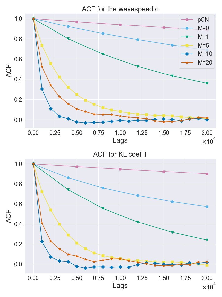
Figure 1: ACF curves for wave speed $c$ and the first KL coefficient.

Integrated autocorrelation time $\div\,1000$
	PCN	$M{=}0$	$M{=}1$	$M{=}5$	$M{=}10$	$M{=}20$
$c$	$360$	$130$	$50$	$7.7$	$\boldsymbol{1.5}$	$4.3$
$\eta_{1}$	$390$	$110$	$30$	$6.8$	$\boldsymbol{1.4}$	$3.1$
$\eta_{5}$	$290$	$46$	$55$	$11$	$\boldsymbol{1.1}$	$1.9$
$\eta_{15}$	$280$	$30$	$16$	$12$	$\boldsymbol{1.0}$	$1.2$
$\eta_{100}$	$310$	$43$	$20$	$11$	$\boldsymbol{1.1}$	$1.4$

Table 2: IATs for wave speed $c$ and several KL coefficients with the fastest IATs in bold. All IATs have been divided by $1000$ to improve readability.

To check that FES remains stable with increasing dimension, we also run our experiments with a discretization into twice as many grid points. The IATs remain statistically indistinguishable from those reported in Table 2 with relative differences of $\leq 10\%$.

Lastly, to help explain why FES performs so much better than PCN, we present Figure 2, which shows posterior samples of $\rho_{0}$ conditioned on several values of $c$. This figure reveals the strong correlation between the wave speed $c$ and the low-wavenumber components of $\rho_{0}$. Since the PCN sampler does not account for this correlation structure, large PCN updates are highly unlikely to be accepted. In contrast, FES naturally adapts to this correlation structure, eliminating the major bottleneck in the sampling.

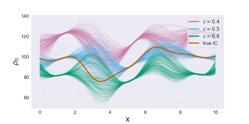
Figure 2: Samples of $\rho_{0}$ conditioned on three values of the wave speed $c$.

4.2 Path reconstruction for Langevin dynamics

We consider a dynamical system in which position $X_{t}$ and momentum $P_{t}$ evolve according to the following Langevin SDE.

$$\begin{cases}\mathop{dX}=P\mathop{dt},&t>0,\\ \mathop{dP}=-\alpha X\mathop{dt}+\sigma\mathop{dW},&t>0,\\ X=P=0,&t=0.\end{cases}$$ (18)

We aim to recover the parameters $\alpha>0$ and $\sigma>0$, as well as the complete path $\left(X_{t}\right)_{0\leq t\leq 10}$, based on noisy observations of position at a few specific times.

We use the following Bayesian priors.

$$\alpha\sim\text{Exp}(12),\quad\sigma\sim\text{Exp}(4),\quad W\sim\text{BM}([0,10]).$$ (19)

As an example of mild model misfit, we set $X_{t}=\sin(4t)$ and then add $\mathcal{N}\left(0,0.09\right)$ observational noise at times $t=1,3,5,7$, and $9$.

To approximate the posterior path distribution, we first infer the driving Brownian motion $\left(W_{t}\right)_{0\leq t\leq 10}$ and the scalar parameters $\log\alpha$ and $\log\sigma$. Then, we recover the posterior path by integrating forward the SDE (18) using a standard Euler solver. To discretize $X_{t}$ and $W_{t}$, we use $200$ equally spaced times between $t=0$ and $t=10$.

We compare the performance of five different MCMC samplers:

1. A PCN-based sampler that simultaneously proposes PCN updates for $W$ and Gaussian random walk updates for $\left(\log\alpha,\log\sigma\right)$.

2. The “hybrid sampler” of zhou2017hybrid , which explicitly estimates the posterior covariance matrix.

3. A modified FES sampler with $L=8$ walkers and joint proposals that combine AIES and PCN moves to update all the parameters at once.

4. A modified FES sampler with $L=100$ walkers and joint proposals.

5. A standard FES sampler with $L=100$ walkers.

We initialize our samplers by drawing randomly from the Bayesian prior distribution. After a short pilot run, we find that $M=5$ is a near-optimal truncation parameter, and we fix this parameter for all the samplers (besides PCN). We report the IATs for the samplers in Table 3, and we show ACF curves in Figure 3.

Integrated autocorrelation times $\div\,1000$
	PCN	Hybrid	Joint, $L{=}8$	Joint, $L{=}100$	$L{=}100$
$\log\alpha$	$51$	$38$	$23$	$\boldsymbol{11}$	$12$
$\log\sigma$	$26$	$22$	$18$	$\boldsymbol{6.6}$	$8.1$
$\eta_{1}$	$5.7$	$1.5$	$6.3$	$\boldsymbol{1.0}$	$1.6$
$\eta_{10}$	$5.9$	$1.6$	$2.8$	$2.0$	$\boldsymbol{0.39}$
$\eta_{100}$	$5.8$	$1.2$	$2.5$	$1.8$	$\boldsymbol{0.30}$

Table 3: IATs for $\log\alpha$, $\log\sigma$, and several KL coefficients with the fastest IATs in bold. All IATs have been divided by $1000$ to improve readibility.

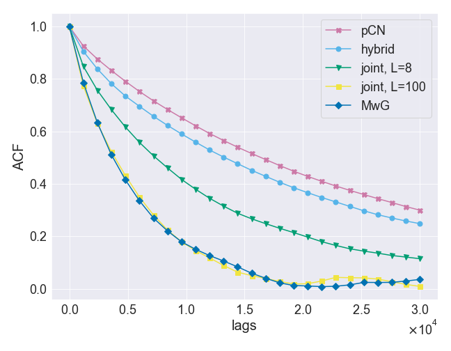
Figure 3: ACF curves for the $\alpha$ parameter

As a first comparison, we find that FES mixes more quickly with $L=100$ walkers than with $L=8$ walkers. $L=8$ is the minimal possible number of walkers to ensure the AIES sampler does not get stuck in a low-dimensional subspace. However, it is recommended to use more walkers whenever possible. Foreman-Mackey and coauthors recommend using hundreds of walkers foreman2013emcee , and in some applications up to 2000 walkers have been used Akeret_CosmoHammer .

As a second comparison, we find that joint updates lead to slightly faster sampling within the AIES subspace but slower sampling in the complementary subspace, compared to standard FES updates. Thus, the advantages of joint updates versus standard Metropolis-within-Gibbs updates depend on the particular statistics being estimated.

As a last comparison, we find that the hybrid sampler of zhou2017hybrid has two shortcomings that can be addressed by using FES. First, the hybrid sampler is very slow to estimate the posterior covariance matrix. Figure 4 reveals that more than a million iterations are needed for the estimated variances for $\log\alpha$ and $\log\sigma$ parameters to stabilize. Since the hybrid sampler tunes its proposals based on the estimated posterior covariance matrix, the method requires over a million iterations to achieve its peak efficiency. In contrast, FES does not require such an adaptation period: the dynamics remain stable from the very first iteration onwards.

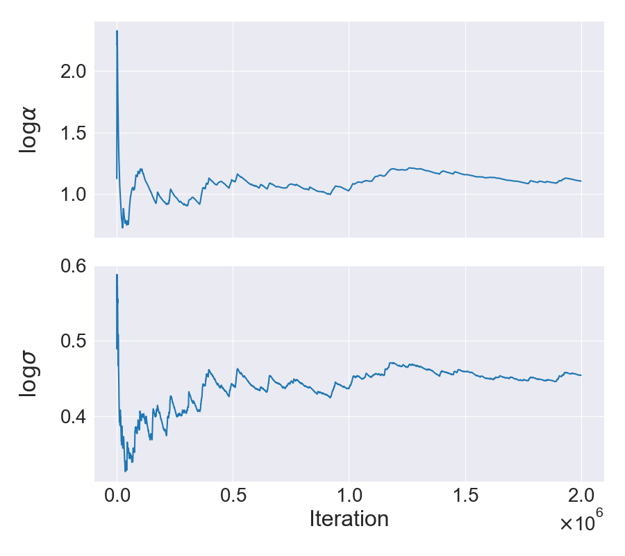
Figure 4: Variance estimates for $\log\alpha$ and $\log\sigma$ using the adaptive hybrid sampler.

Second, even after the hybrid sampler has adapted to the posterior covariance structure, mixing times for all observable are still comparatively slow. A major obstacle limiting the efficiency of the hybrid sampler is the multimodality of the posterior distribution, which is highlighted in Figures 5 and 6. It is very challenging for a Gaussian random walk to efficiently traverse a multimodal distribution. In contrast, we find in this example that FES significantly outperforms the hybrid sampler, suggesting a robustness to multimodality that is highly desirable in applications.

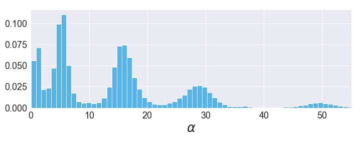
Figure 5: Posterior pdf for $\alpha$ exhibiting multimodality.

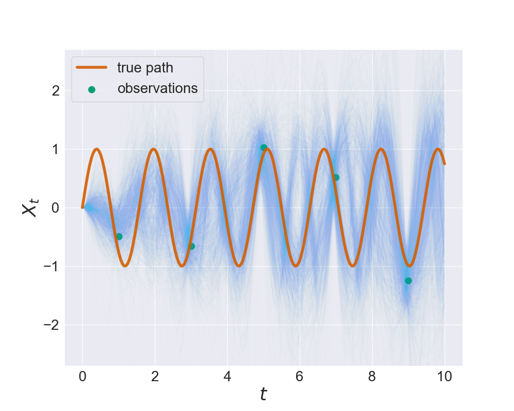
Figure 6: Posterior paths exhibiting multimodality.

5 Conclusion

In this work, we introduced the functional ensemble sampler (FES). FES requires no gradients, it is easy to code, and it is parallelizable. These factors make FES a widely applicable sampler for infinite-dimensional inverse problems.

In two numerical examples, we demonstrated the benefits of using FES. First, when parameters in the posterior distribution are highly correlated, we showed how FES can reduce integrated autocorrelation times by two orders of magnitude compared to PCN. Second, when the posterior distribution is mildly multimodal, we showed how FES outperforms PCN and the alternative gradient-free sampler of zhou2017hybrid .

We acknowledge two opportunities to improve the performance of FES even further. First, FES sampling could be streamlined by identifying a likelihood-informed subspace where enhanced sampling is most essential. Second, after isolating a low-dimensional subspace for enhanced sampling, we find that FES is typically an efficient sampler, except in cases of extreme multimodality in which FES deteriorates in its performance goodman2010ensemble and further sampling modifications may be needed.

In conclusion, FES pushes the limits of the MCMC approach to solving infinite-dimensional inverse problems. Despite having a few limitations, the method offers a practical and powerful solution for many sampling problems where PCN falls short, and we recommend FES as a general-purpose gradient-free sampler.

- (1) Akeret, J., Seehars, S., Amara, A., Refregier, A., Csillaghy, A.: Cosmohammer: Cosmological parameter estimation with the MCMC hammer. Astronomy and Computing 2, 27–39 (2013)
- (2) Beskos, A., Girolami, M., Lan, S., Farrell, P.E., Stuart, A.M.: Geometric MCMC for infinite-dimensional inverse problems. Journal of Computational Physics 335, 327–351 (2017)
- (3) Beskos, A., Jasra, A., Law, K., Marzouk, Y., Zhou, Y.: Multilevel sequential Monte Carlo with dimension-independent likelihood-informed proposals. SIAM/ASA Journal on Uncertainty Quantification 6(2), 762–786 (2018)
- (4) Beskos, A., Roberts, G., Stuart, A., Voss, J.: MCMC methods for diffusion bridges. Stochastics and Dynamics 8(03), 319–350 (2008)
- (5) Chen, Y., Keyes, D., Law, K.J., Ltaief, H.: Accelerated dimension-independent adaptive Metropolis. SIAM Journal on Scientific Computing 38(5), S539–S565 (2016)
- (6) Cotter, S.L., Roberts, G.O., Stuart, A.M., White, D.: MCMC methods for functions: Modifying old algorithms to make them faster. Statistical Science pp. 424–446 (2013)
- (7) Coullon, J., Pokern, Y.: MCMC for a hyperbolic Bayesian inverse problem in traffic flow modelling. arXiv preprint arXiv:2001.02013 (2020)
- (8) Cui, T., Law, K.J., Marzouk, Y.M.: Dimension-independent likelihood-informed MCMC. Journal of Computational Physics 304, 109–137 (2016)
- (9) Cui, T., Martin, J., Marzouk, Y.M., Solonen, A., Spantini, A.: Likelihood-informed dimension reduction for nonlinear inverse problems. Inverse Problems 30(11), 114,015 (2014)
- (10) Dunlop, M.M., Stuart, A.M.: The Bayesian formulation of EIT: Analysis and algorithms. Inverse Problems and Imaging 10(4), 1007–1036 (2016)
- (11) Foreman-Mackey, D., Hogg, D.W., Lang, D., Goodman, J.: emcee: the MCMC hammer. Publications of the Astronomical Society of the Pacific 125(925), 306 (2013)
- (12) Goodman, J., Weare, J.: Ensemble samplers with affine invariance. Communications in Applied Mathematics and Computational Science 5(1), 65–80 (2010)
- (13) Hairer, M., Stuart, A.M., Vollmer, S.J., et al.: Spectral gaps for a Metropolis–Hastings algorithm in infinite dimensions. Annals of Applied Probability 24(6), 2455–2490 (2014)
- (14) Hu, Z., Yao, Z., Li, J.: On an adaptive preconditioned Crank–Nicolson MCMC algorithm for infinite dimensional Bayesian inference. Journal of Computational Physics 332, 492–503 (2017)
- (15) Iglesias, M.A., Lin, K., Stuart, A.M.: Well-posed Bayesian geometric inverse problems arising in subsurface flow. Inverse Problems 30(11), 114,001 (2014). DOI 10.1088/0266-5611/30/11/114001. URL https://doi.org/10.1088%2F0266-5611%2F30%2F11%2F114001
- (16) Kantas, N., Beskos, A., Jasra, A.: Sequential Monte Carlo methods for high-dimensional inverse problems: A case study for the Navier-Stokes equations. SIAM/ASA Journal on Uncertainty Quantification 2(1), 464–489 (2014)
- (17) Law, K.J.: Proposals which speed up function-space MCMC. Journal of Computational and Applied Mathematics 262, 127–138 (2014)
- (18) Metropolis, N., Rosenbluth, A.W., Rosenbluth, M.N., Teller, A.H., Teller, E.: Equation of state calculations by fast computing machines. Journal of Chemical Physics 21(6), 1087–1092 (1953)
- (19) Roberts, G.O., Rosenthal, J.S.: Examples of adaptive MCMC. Journal of Computational and Graphical Statistics 18(2), 349–367 (2009)
- (20) Rudolf, D., Sprungk, B.: On a generalization of the preconditioned Crank–Nicolson Metropolis algorithm. Foundations of Computational Mathematics 18(2), 309–343 (2018)
- (21) Sokal, A.: Monte Carlo methods in statistical mechanics: Foundations and new algorithms. In: Functional integration, pp. 131–192. Springer (1997)
- (22) Stuart, A.M.: Inverse problems: a Bayesian perspective. Acta Numerica 19, 451 (2010)
- (23) Zhou, Q., Hu, Z., Yao, Z., Li, J.: A hybrid adaptive MCMC algorithm in function spaces. SIAM/ASA Journal on Uncertainty Quantification 5(1), 621–639 (2017)