Non-abelian Thouless pumping in a photonic lattice

Abstract

Non-abelian gauge fields emerge naturally in the description of adiabatically evolving quantum systems having degenerate levels. Here we show that they also play a role in Thouless pumping in the presence of degenerate bands. To this end we consider a photonic Lieb lattice having two degenerate non-dispersive modes and show that, when the lattice parameters are slowly modulated, the propagation of the photons bear the fingerprints of the underlying non-abelian gauge structure. The non-dispersive character of the bands enables a high degree of control on photon propagation. Our work paves the way to the generation and detection of non-abelian gauge fields in photonic and optical lattices.

To describe the dynamics of a quantum system whose Hamiltonian depends on some external classical parameters in the energy eigenstate basis, one is naturally led to introduce a gauge field bott1965 that keeps track of how the eigenstates transform in parameters space. As first noted by Simon simon1983 , the Berry’s phase berry1984 is the holonomy associated with this gauge structure when the evolution of the system takes place in an isolated non-degenerate eigenstate. If the evolution involves a degenerate energy eigenspace the underlying gauge theory becomes non-abelian wilczek1984 .
Among the most fascinating and studied manifestations of Berry’s curvature wilczek1989 ; resta2007 are those that involve transport with the closely related phenomena of quantum Hall effect thouless1982 and Thouless pumping thouless1983 . Thouless pumping refers to the transport of charge in the absence of any external bias by cycling adiabatically in time a one-dimensional lattice potential confining the charge. It is considered as a natural probe of Berry’s geometric phase aunola2003 ; mottonen2006 ; xiao2010 ; zilberberg2018 ; PhysRevB.93.245113 ; Aidelsburger2014 and of the Chern numbers thouless1983 ; kraus2012 ; ke2016 ; wimmer2017 ; fedorova2019 ; wang2019 ; lohse2015 ; nakajima2016 ; kremer2020 .

Here we show that, in the presence of degenerate bands, Thouless pumping can be exploited to probe the underlying non-abelian gauge structure. The non-abelian analogue of the Berry’s phase, the holonomy of Wilczek and Zee wilczek1984 , keeps track of how the degenerate subspace deforms along a path in parameters space and it depends on the geometric and topological structure of the Hilbert space. We establish a relation between the Wilczek and Zee holonomy and Thouless pumping.

To exemplify our findings we consider a simple one-dimensional lattice model that we name for simplicity non-abelian Lieb chain (naL) since it is reminiscent of the two-dimensional Lieb lattice model lieb1989 , recently at the focus of pioneering experiments on light confinement in photonic waveguide lattices vicencio2015 ; mukherjee2015 . We show that the slow cyclic modulation of the model parameters yields a current that can be directly connected to the holonomy generated during the cycle. The non-abelian Lieb chain can be experimentally realized in a photonic waveguide lattice and the non-abelian holonomy can be read-out from the photon beam displacement along its propagation. Our results thus point at a straightforward approach to generate and detect Wilczek-Zee non-abelian holonomies. In this respect, we remark that, in spite of a few theoretical proposals duan2001 ; taddia2017 ; faoro2003 ; brosco2008 ; pachos2000 ; iadecola2016 ; chen2019 , only two experimental verifications of Wilczek-Zee non-abelian holonomies exist so far, namely, the pioneering nuclear quadrupole resonance experiment of Ref.[zwanziger1990, ] and the circuit QED martinis2020 implementation of Abdumalikov et al.abdumalikov2013 .

Photonic waveguide lattices are the ideal playground to realize topological lattice models ozawa2019 . In these systems, consisting of arrays of evanescently coupled single-mode waveguides christodoulides2003 , light propagation can be modeled by means of a Schrödinger equation where the role of time is played by the coordinate along the waveguide, $z$, and the Hamiltonian describes the hopping of bosonic particles across the array. Such lattice-based description has long been applied to describe light propagation in photonic waveguides arrays and it can be derived using coupled-mode theory, as discussed in various textbooks snyder and briefly outlined in Section IV. To implement Thouless pumping, the diagonal elements of the lattice Hamiltonian, can be modulated along $z$ by tuning the waveguide diffraction index and the lateral confinement length, while the hopping matrix elements can be controlled by changing the overlap of the evanescent tails of neighboring waveguides, e.g. modifying the lattice spacings. Recently, modulated photonic waveguides were employed to implement adiabatic population transfer PhysRevResearch.1.033117 in a tripod system corresponding to a single unit cell of the naL lattice proposed below.

The paper is organized as follows. After introducing the naL chain model in Section I, we present our main results concerning the relation between Wilczek-Zee holonomy and Thouless pumping in Section II, eventually, in Sections III and IV we illustrate the results starting from specific examples of pumping cycles. In section IV we outline the derivation of the lattice model equations from coupled mode theory, we discuss some experimental requirements to discern genuine geometric effects from non-adiabatic transitions.

I Non-abelian Lieb chain

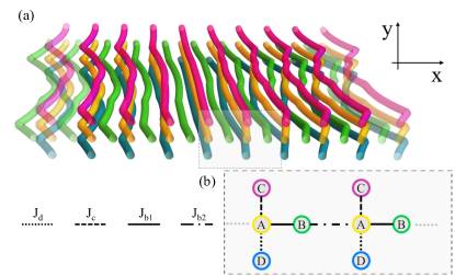
Figure 1: a) Illustration of the waveguides array with z-dependent couplings. b) Structure of the non-abelian waveguide lattice which features two dispersive and two degenerate flat bands.

The naL chain consists of a one-dimensional lattice with four sites per unit cell, indicated respectively as $A$, $B$, $C$ and $D$. As shown in Fig.1, the lattice lies in the $(x,\,y)$-plane and it has two dangling bonds in each unit cell, it is an extension of the one-dimensional Lieb lattice considered in Refs.[casteels2016, ; biondi2018, ]. The inter- and intra- cell hopping amplitudes along $x$ are indicated as $J_{b1}$ and $J_{b2}$ while $J_{c}$ and $J_{d}$ denote the hopping amplitudes along the dangling bonds. The Hamiltonian thus reads as follows

$$H_{\rm naL}\!=\!\!\!\sum_{i}\!\left(J_{b1}a^{\dagger}_{i}b_{i}+J_{b2}a^{\dagger}_{i}b_{i-1}+J_{c}a^{\dagger}_{i}c_{i}+J_{d}a^{\dagger}_{i}d_{i}+{\rm H.c.}\right)$$ (1)

where $a_{i},\,b_{i},\,c_{i},\,d_{i}$ and $a^{\dagger}_{i},\,b^{\dagger}_{i},\,c^{\dagger}_{i},\,d^{\dagger}_{i}$ are bosonic annihilation and creation operators on the $A$, $B$, $C$ and $D$ sites of cell $i$. Switching to $k$-space we can recast $H_{\rm naL}$ as follows

$$H_{\rm naL}=\sum_{k}\!\left(J_{b}a^{\dagger}_{k}b_{k}+J_{c}a^{\dagger}_{k}c_{k}+J_{d}a^{\dagger}_{k}d_{k}+{\rm H.c.}\right)$$ (2)

where $a_{k},\,b_{k},\,c_{k}$ and $d_{k}$ denote $k$-space creation and annihilation operators and $J_{b}=J_{b1}+J_{b2}e^{ik}$.

Thouless pumping requires the cyclic modulation of the parameters defining the lattice potential. Clearly, rather than a charge current, photonic lattice pumping yields a $z$-dependent displacement of the photon beam across the lattice ke2016 ; wimmer2017 ; fedorova2019 ; wang2019 . Specifically, assuming that the system is initialized in a Wannier state, the role of the pumped charge is played by the displacement of the Wannier center, whose geometric and topological significance, was first elucidated in the context of polarization theory resta2007 . Below we establish a general relation between displacement and non-abelian holonomies.

II Displacement and holonomies

As schematically shown in Fig.1a), we assume that the hopping amplitudes, $J_{\mu}$ with $\mu=b1,b2,c,d$ are periodic functions of the longitudinal coordinate $z$ and we indicate with $\lambda_{0}$ the wavelength of their modulation.

To calculate the photon beam displacement, $\Delta x$, generated along a cycle we start from the following general expression

$$\Delta x=\int_{0}^{\lambda_{0}}\partial_{z}(\langle\psi(z)|\hat{x}|\psi(z)\rangle)dz$$ (3)

where $|\psi(z)\rangle$ indicates the electromagnetic field’s amplitude, solution of a Schrödinger equation of the form bra-ket ,

$$i\partial_{z}|\psi(z)\rangle=H_{\rm naL}(z)|\psi(z)\rangle$$ (4)

and $\hat{x}$ denotes the position operator. Assuming that $\lambda_{0}$ is the largest relevant length-scale, in the adiabatic limit, a suitable basis to expand the field $|\psi(z)\rangle$ is the Bloch eigenmodes basis, $\{|\psi_{\nu a}(k,z)\rangle\}$, that diagonalizes the naL Hamiltonian for each value of $k$ and $z$. See Appendix A for more details. It consists of two dispersive modes with longitudinal momenta $\kappa_{\pm}(k)=\pm\Delta(k)$, $\Delta(k)=\sqrt{|J_{b}(k)|^{2}+J_{c}^{2}+J_{d}^{2}}$ and two dispersionless degenerate modes, $|\psi_{01}\rangle$ and $|\psi_{02}\rangle$, with longitudinal momentum $\kappa_{0}=0$, defined as

$$|\psi_{01}\rangle = \frac{J_{c}|d_{k}\rangle-J_{d}|c_{k}\rangle}{\delta}$$ (5)

$$|\psi_{02}\rangle = \frac{\delta^{2}|b_{k}\rangle+J_{b}^{*}(J_{c}|c_{k}\rangle+J_{d}|d_{k}\rangle)}{\delta\Delta(k)}$$ (6)

with $\delta=\sqrt{J_{c}^{2}+J_{d}^{2}}$.

To keep the discussion general, we assume that the system is initialized, at $z=z_{0},$ in the Wannier state centered at the site $n$ belonging to the mode $\kappa_{\nu}$, we thus set

$$|\psi(z_{0})\rangle=|w_{\nu a}(n,z_{0})\rangle=\sum_{ka}c_{a}|\psi_{\nu a}(k,z_{0})\rangle e^{ikn}$$ (7)

where $k$ runs over the reciprocal lattice sites, $\nu=0,\pm$ and the subscript $a$, not to be confused with the operator $a$, enumerates the basis states within the degenerate subspace, i.e. $a\in[1,\ldots,d_{\nu}]$ with $d_{\nu}$ indicating the dimension of the degenerate modes subspace. For the naL lattice we have $d_{0}=2$ and $d_{+}=d_{-}=1$.

Since the modulation of the lattice parameters preserves the translational invariance of the lattice for all $z$, the quasi-momentum, $k$, is a good quantum number both in the driven and undriven system and the adiabatic evolution operator, $U(z,z_{0})$, can be factorized as follows

$$U(z,z_{0})\simeq\prod_{\mu k}{\cal U}_{\mu k}(z,z_{0}).$$ (8)

In the above equation ${\cal U}_{\mu k}(z,z_{0})$ describes the evolution starting from a local Bloch eigenmode with quasi-momentum $k$ and longitudinal momentum $\kappa_{\mu}$,

$${\cal U}_{\mu k}(z,z_{0})=\sum_{ab}\left[W_{\mu}\right]_{ab}(z,z_{0})|\psi_{\mu a}(k,z)\rangle\langle\psi_{\mu b}(k,z_{0})|$$ (9)

where the symbol $[\dots]_{ab}$ denotes the $ab$ element of the matrix inside the brackets, $a$ and $b$ span a degenerate subset and $W_{\mu}(z,z_{0})$ is wilczek1984 :

$$W_{\mu}(z,z_{0})=e^{i\!\int_{z_{0}}^{z}\!\kappa_{\mu}(z)dz}\,{\cal P}\exp\left[i\!\int_{z_{0}}^{z}\!\Gamma^{z}_{\mu}dz\right]$$ (10)

with ${\cal P}$ denoting the path-ordering and $\Gamma^{z}_{\mu}$ indicating the Wilczek-Zee connection,

$$\left[\Gamma^{z}_{\mu}\right]_{ab}=\langle\psi_{\mu a}(k,z)|i\partial_{z}|\psi_{\mu b}(k,z)\rangle.$$ (11)

When $\kappa_{\mu}$ corresponds to a single non-degenerate mode, $\Gamma^{z}_{\mu}$ reduces to the standard Berry’s connection.

Using the adiabatic evolution operator defined in equations (8-11) and the initial condition given in Eq.(7), we obtain the following expression for the field at $z=z_{1}>z_{0}$ in the adiabatic limit

$$|\psi(z_{1})\rangle=\sum_{kab}c_{a}\left[W_{\nu}(z_{1},z_{0})\right]_{ba}|\psi_{\nu b}(k,z_{1})\rangle e^{ikn}.$$ (12)

From the above equation, it correctly emerges that the adiabatic dynamics in the presence of $N$ degenerate modes is invariant under $z$-dependent changes of basis in the degenerate subset, i.e. $SU(N)$ gauge transformations. Consequently, $W$ transforms as:

$$W(z,z_{0})\rightarrow M^{{\dagger}}(z)W(z,z_{0})M(z_{0})$$

and for cyclic transformations it behaves as a rank 2 tensor. It yields, apart from an irrelevant phase factor, the Wilson loop, $W(\lambda_{0},0)$, on the fiber bundle that is locally the product of the $z$-varying parameters space and the degenerate modes subset.

Replacing Eq.(12) in Eq.(3), we can derive a transparent and simple expression for the displacement introducing the non-abelian connection along $k$, i.e. $\left[\Gamma^{k}_{\nu}\right]_{ab}=\langle\psi_{\nu a}|i\partial_{k}|\psi_{\nu b}\rangle$, that is the non-abelian version of the Zak phase zak1989 . By doing so, following the derivation described below, we arrive at our final expression for the photon beam displacement:

$$\Delta x=\sum_{ab}c^{*}_{a}c_{b}D^{\nu}_{ab}\,,$$ (13)

where the displacement matrix $D^{\nu}_{ab}$ can be expressed as follows

$$D^{\nu}_{ab}=\frac{1}{2\pi}\int_{0}^{\lambda_{0}}\!\!\!dz\int_{-\pi}^{\pi}\!\!\!\!dk\left[W^{\dagger}_{\nu}\,{\cal F}^{\nu}_{kz}W_{\nu}\right]_{ab}$$ (14)

with ${\cal F}^{\nu}_{kz}=\partial_{k}\Gamma^{z}_{\nu}-\partial_{z}\Gamma^{k}_{\nu}+i\left[\Gamma^{z}_{\nu},\Gamma^{k}_{\nu}\right]$ denoting the non-abelian field strength matrix.

Equations (13-14) relate the photon beam displacement to the non-abelian holonomy generated along a cycle when the evolution involves a degenerate eigenmodes subspace. It clearly shows that in general, the displacement, $\Delta x$, will bear the consequence of the non-abelian nature of the dynamics while it yields the known abelian result when $d_{\nu}=1$. Comparing Eqs. (13-14) to their abelian counterpart resta2007 ; thouless1983 , one easily realizes that the displacement matrix can be viewed as the flux of the non-abelian field strength, ${\cal F}^{\nu}_{kz}$, that transforms along the path with the path-dependent factors $W^{\dagger}_{\nu}$ and $W_{\nu}$ as prescribed by the non-abelian Stokes theorem fishbane1981 . As shown in Ref. [fishbane1981, ], the presence of these factors ensures that the surface integral is independent on the choice of the surface. Furthermore it guarantees that the displacement matrix, $D^{\nu}_{ab}$, transforms as a rank-2 tensor under gauge transformation and consequently that the total displacement given by Eq. (13) is gauge-invariant.

Before proceeding further, we present a derivation of Eqs. (13-14). To start with we express the position operator $\hat{x}$ in $k$-space as follows,

$$\hat{x}=\sum_{m,k}|m_{k}\rangle\langle m_{k}|i\partial_{k},$$ (15)

where $m=a,b,c,d$. Inserting (15) in Eq.(3) and using Eq.(12) and (13) we can rewrite the displacement matrix as follows

$$D^{\nu}_{ab} = \frac{1}{2\pi}\int_{0}^{\lambda_{0}}\int_{0}^{2\pi}\!\!\partial_{z}\left[W^{\dagger}_{\nu}(z,z_{0})\langle\Psi_{\nu}(k,z)|\right.$$

$$\left.i\partial_{k}\left(|\Psi_{\nu}(k,z)\rangle W_{\nu}(z,z_{0})\right)\right]_{ab}\,dk\,dz$$

where we introduced the vector notation, i.e. $|\Psi_{\nu}\rangle=(|\psi_{\nu 1}\rangle,...,|\psi_{\nu d_{\nu}}\rangle)$. Expanding the derivatives in equation (LABEL:dim1) we obtain:

$$D^{\nu}_{ab} = \frac{1}{2\pi}\int_{0}^{\lambda_{0}}\!\!\!dz\int_{0}^{2\pi}\!\!\!\!dk\left[\partial_{z}\left(W_{\nu}^{\dagger}\left<\Psi_{\nu}\right|\,i\partial_{k}\,\left|\Psi_{\nu}\right>W_{\nu}\right)+\right.$$

$$\left.+i\partial_{z}\left(W_{\nu}^{\dagger}\right)\,\partial_{k}\,W_{\nu}+iW_{\nu}^{\dagger}\,\partial_{k}\partial_{z}\,W_{\nu}\right]_{ab}$$

The $z$-derivatives of the operators $W_{\nu}$ and $W^{\dagger}_{\nu}$ are given by:

$$\partial_{z}W_{\nu} = i(\Gamma_{\nu}^{z}+\kappa_{\mu}I)\,W_{\nu}$$ (18)

$$\partial_{z}W^{\dagger}_{\nu} = -iW_{\nu}^{\dagger}\,(\Gamma_{\nu}^{z}+\kappa_{\mu}I)$$ (19)

where $\Gamma_{\nu}^{z}$ is the non-abelian connection defined in Eq.(11). Substituting these relations in Eq.(LABEL:dim2) we obtain:

$$D^{\nu}_{ab} = \frac{1}{2\pi}\int_{0}^{\lambda_{0}}\!\!\!dz\int_{-\pi}^{\pi}\!\!\!\!dk\left[-W^{\dagger}_{\nu}\,\partial_{k}\left(\Gamma_{\nu}^{z}+\kappa_{\mu}I\right)W_{\nu}+\right.$$ (20)

$$\left.-\partial_{z}\left(W_{\nu}^{\dagger}\Gamma_{k}W_{\nu}\right)\right]_{ab}.$$

Using again Eqs.(18-19) to express the $z$-derivatives and using the definition of ${\cal F}_{zk}$ and the $k$-periodicity of $\kappa_{\mu}$, we easily recover Eq. (14).

III Pumping cycles

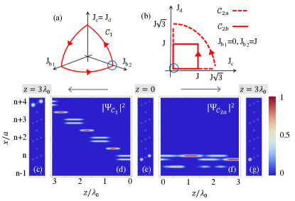
Figure 2: (a-b) Examples of pumping cycles. The blue circle indicates their starting point, $z=z_{0}$. Note that we take a small but finite values of $J_{c}=J_{d}$ at $z=z_{0}$ to avoid ambiguities in the definition of the eigenstates. Along ${\cal C}_{1}$ we have $J_{d}=J_{c}$ while along ${\cal C}_{2(a-b)}$ we have $J_{b2}=J,J_{b1}=0$. (c-g) Numerically evaluated field’s intensity along ${\cal C}_{1}$ and ${\cal C}_{2a}$ with $\lambda_{0}J=200$, panels (c) and (g) show the field intensity in the final states after three cycles $C_{1}$ and after three cycles $C_{2a}$. To allow a clearer identification, in all panels we slightly displaced the sites “C” and “D” along $x$.

To further understand the non-commutative nature of pumping in the naL chain, it is useful to consider some specific example. In Fig. 2(a-b) we show three pumping cycles, ${\cal C}_{1}$, ${\cal C}_{2a}$ and ${\cal C}_{2b}$. As one can see, the cycle ${\cal C}_{1}$ defines a spherical triangle in parameters space while the cycles ${\cal C}_{2a}$ and ${\cal C}_{2b}$ are contained in the plane $J_{b2}=J$ and $J_{b1}=0$ and they involve only the manipulation of $J_{c}$ and $J_{d}$. The blue circle indicates the point where we start covering the cycles at $z=z_{0}$. The corresponding holonomy transformations can be written as, (see Appendix C for more details)

$$W_{{{\cal C}_{1}}}=e^{i\frac{k}{2}\left(\sigma_{0}-\sigma_{z}\right)}\,\,{\rm and}\,\,W_{{\cal C}_{2i}}=e^{i\Delta_{{\cal C}_{2i}}\!\left(\sin(k)\sigma_{x}+\cos(k)\sigma_{y}\right)}$$ (21)

where $\sigma_{x},\,\sigma_{y},\,\sigma_{z}\,\,{\rm and}\,\,\sigma_{0}$ denote respectively the Pauli matrices and the $2\times 2$ identity matrix and the angles $\Delta_{{\cal C}_{2i}}$ depend on the precise shape of the cycles ${\cal C}_{2i}$. The above expressions hold in the basis of Bloch eigenmodes at $z=z_{0}$. Using Eqs. (5-6), the latter can be shown to satisfy the following simple relations: $|\psi_{01}\rangle\propto|d_{k}\rangle-|c_{k}\rangle$ and $|\psi_{02}\rangle\propto|d_{k}\rangle+|c_{k}\rangle.$ From Eq. (21) we thus see, that in the adiabatic limit, the cycle ${\cal C}_{1}$ does not affect the antisymmetric mode, $|\psi_{01}\rangle$, while it simply multiplies the symmetric mode, $|\psi_{02}\rangle$, times the phase factor $e^{ik}$. The cycles ${\cal C}_{2a}$ and ${\cal C}_{2b}$ instead yield a rotation in the degenerate subspace by an angle $\Delta_{{\cal C}_{2i}}$ such that $\Delta_{{\cal C}_{2a}}=\pi/4$ and $\Delta_{{\cal C}_{2b}}=\pi/6$, as shown in Appendix C.

These approximate analytical results are in good agreement with the numerical results, shown in Figures 2(c-g), obtained by solving Eq.(4) on a finite lattice. There we plot the field’s intensity as a function of $z$ and $x$ during the application of three consecutive cycles ${\cal C}_{1}$, Fig.2(d), and in the final state at $z=3\lambda_{0}$, Fig.2(c). Analogous plots for the cycle ${\cal C}_{2a}$ are shown in Fig.2(f-g). In both cases the system is initialized in the Wannier state $|w_{02}(n,z_{0})\rangle$, corresponding to the symmetric mode, as shown Fig. 2(e) displaying the field’s intensity at $z=z_{0}$. Comparing Fig. 2(c) and Fig. 2(e) we see that the application of three cycles ${\cal C}_{1}$ displaces the initial state forward by three unit cells. On the contrary the application of three cycles ${\cal C}_{2a}$ yields a $3/4\pi$ rotation but zero displacement, thus the initial state $|c_{n}\rangle+|d_{n}\rangle$ is rotated into the state $|c_{n}\rangle$ as shown in Fig. 2(g).

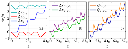
Figure 3: Photon beam displacement for a) the cycles ${\cal C}_{1}$ (middle line), ${\cal C}_{2a}$ (lower line) and ${\cal C}_{2b}$ (upper line) and b) the sequential application of ${\cal C}_{1}$ and ${\cal C}_{2a}$: ${\cal C}_{2a}{\cal C}_{1}$ (upper line) and ${\cal C}_{1}{\cal C}_{2a}$ (lower line). c) Trace of the displacement matrix for the sequences ${\cal C}_{2a}{\cal C}_{1}$ (upper line) and ${\cal C}_{1}{\cal C}_{2a}$ (lower line).

The difference between the cycles ${\cal C}_{1}$, ${\cal C}_{2a}$ and ${\cal C}_{2b}$ can be also appreciated in Fig. 3. There we plot the displacement evaluated numerically from equation (3) for the system initially prepared in the state $|w_{02}(n,z_{0})\rangle$ as a function of $z$ for the different cycles. In panel (a) we see that the displacement generated along the cycle ${\cal C}_{1}$ is quantized. This is a natural consequence of the structure of the holonomy matrix, given in Eq. (21), that leads to the following simple expression for the displacement matrix $D^{0}_{{\cal C}_{1}}=\left(\begin{array}[]{cc}0&0\\ 0&1\\ \end{array}\right),$ as discussed in details in Appendix C.

This quantization reflects the topological nature of Thouless pumping that in the non-abelian case implies, ${\rm Tr}[D^{\nu}_{\cal C}]=C^{1}_{\nu}$ where $C^{1}_{\nu}$ denotes the first Chern number of the degenerate band $\nu$ manton2004 .

As shown in Fig. 3(b), the situation is rather different if we perform a sequence of the cycles ${\cal C}_{1}$ and ${\cal C}_{2a}$. In this case the non-abelian nature of the evolution manifests in a non-integer displacement per cycle and in the dependence of the generated displacement on the ordering of the sequence. Focusing on the sequence ${\cal C}_{1}{\cal C}_{2a}$ we see that starting from the state $|w_{02}(n,z_{0})\rangle$ we get a unitary displacement; for the other ordering, first ${\cal C}_{2a}$ and then ${\cal C}_{1}$, the displacement equals 1/2. The perfect quantization can be recovered by considering the trace of the displacement matrixQianqian2020 ; Cerjan2020 , i.e. the sum of the displacement generated starting in the state $|w_{02}(n,z_{0})\rangle$ and $|w_{01}(n,z_{0})\rangle$. This is exactly what can be seen in Fig. 3(c) where we plot the evolution as a function of $z$ of the traces of the displacement matrices for the sequences ${\cal C}_{2a}{\cal C}_{1}$ and ${\cal C}_{1}{\cal C}_{2a}$, denoted as $Q_{{\cal C}_{2a}{\cal C}_{1}}$ and $Q_{{\cal C}_{1}{\cal C}_{2a}}$.

Non-commutative effects can be detected in various ways in the evolution of the field. For example, one could design a complex pumping cycle aimed at detecting the contribution of the commutator term in the non-abelian Berry’s curvature and consequently the difference between the abelian and non-abelian prediction for the pumped charge. Here, we follow an alternative route, namely we consider the simple cycles ${\cal C}_{2i}$ and ${\cal C}_{1}$ and we show how the non-abelian nature of the dynamics may be detected by changing the order of the cycles.

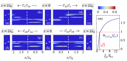
Figure 4: (a-l) Numerically evaluated field’s intensity along different cycles sequences involving ${\cal C}_{1}$, ${\cal C}_{2a}$ and ${\cal C}_{2b}$. For non-commuting cycles the final state depends on the ordering of the sequence. Parameters as in Fig. 2. (m) Distance between the final states obtained with ${\cal C}_{1}{\cal C}_{2a}$ and with ${\cal C}_{2a}{\cal C}_{1}$. The evolution along the sequence ${\cal C}_{2a}{\cal C}_{1}$, i.e. from panel (c) to panel (e) is shown dynamically in the video NAevolution.mp4.

To this end, in Fig.4(a-l) we plot the field intensities as a function of $z$ for different cycles sequences and different orderings. As expected, we see that, when the cycles generate non-commuting holonomies, the final state depends on the ordering of the cycles, as shown in Figs. 4(a-e) for the cycles ${\cal C}_{1}$ and ${\cal C}_{2a}$. Specifically, we see that performing the sequence ${\cal C}_{2a}{\cal C}_{1}$, the initial state, proportional to $|c_{n}\rangle+|d_{n}\rangle$, is first displaced and subsequently rotated by $\pi/4$ yielding the final state $|c_{n+1}\rangle$, Fig. 4(d-e). In the opposite case, ${\cal C}_{1}{\cal C}_{2a}$, the state is first $\pi/4$-rotated and subsequently displaced through the cycle ${\cal C}_{1}$, the final state is thus a linear combination of $|c_{n}\rangle-|d_{n}\rangle$ and $|c_{n+1}\rangle+|d_{n+1}\rangle$. On the contrary, when the holonomies of the two cycles commute, the final state does not depend on the ordering of the cycles, as shown for the cycles ${\cal C}_{2a}$ and ${\cal C}_{2b}$ in Figs. 4(f-l).

A figure of merit, $\Theta$, to characterize the efficiency in generating non-abelian effects may be thus defined from the distance between the final states obtained performing the sequence of two cycles in opposite orders, i.e. $\Theta_{{{\cal C}_{1}{\cal C}_{2i}}}=\sum_{n,m}\left(|\langle m_{n}|\psi_{{\cal C}_{1}{\cal C}_{2i}}\rangle|-|\langle m_{n}|\psi_{{\cal C}_{2i}{\cal C}_{1}}\rangle|\right)^{2}$ where $m$ and $n$ enumerate respectively the sites in a unit cell and the unit cells in the lattice. The value of $\Theta$ will be affected in particular by the shape of the cycle and by the initial conditions. In Figure 4(m) we show the dependence of $\Theta_{{\cal C}_{1}{\cal C}_{2a}}$ on the maximum value, $J_{\rho}$, acquired by $J_{c}$ and $J_{d}$ in the cycle ${\cal C}_{2a}$, that was previously set to $J_{b2}\sqrt{3}$ with $J_{b2}=J$. We see that $\Theta$ increases as we increase $J_{\rho}$ tending towards its maximum value equal to 2. The latter is reached asymptotically when $C_{2a}$ yields a rotation of $\pi/2$. Further discussion of these effects can be found in Appendix C.

So far we considered an idealized situation. Various effects may disturb Thouless pumping, such as non-linearity, non-adiabatic effects and disorder. In Fig. 5 we consider the effects of disorder, the latter may cause a non-perfect periodicity of the lattice enabling transition between different Bloch states, it may distort pumping cycles or break the lattice Hamiltonian symmetries. To exemplify the effects of disorder in Fig. 5 we show the evolution of the field intensity along the cycle ${\cal C}_{1}$ in the presence of impurities of different strengths, yielding the following correction to the Hamiltonian, $\delta H=\sum_{i}\delta\kappa_{i}(c^{\dagger}_{i}c_{i}-d^{\dagger}_{i}d_{i})$. We see that as long as $\delta\kappa_{i}\lambda_{0}\ll 1$, Fig. 5(c), pumping is not affected by the presence of impurities. In the opposite limit $\delta\kappa_{i}\lambda_{0}\gg 1$, the modulation is adiabatic also compared to the splitting introduced by the impurity potential, we thus see in Fig. 5(a) that during the pumping cycle the field intensity follows the impurity profile but the whole process does not cause dispersion or non-adiabatic transitions. Eventually, in the case $\delta\kappa_{i}\lambda_{0}\sim 1$ disorder couples the symmetric and antisymmetric modes, causing imperfections and leakage of Thouless pumping. We note however that the non-abelian Lieb chain offer an advantage over its abelian version. Indeed, since the degenerate bands of the naL lattice are flat, for any kind of modulation dispersive effects, that may hinder the observation of Thouless pumping, are vanishing.

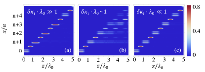
Figure 5: (a-c) Effects of disorder on Thouless pumping. Evolution of the field’s intensity along the cycle ${\cal C}_{1}$ for different disorder strengths: (a) $\delta\kappa_{i}\lambda_{0}\sim 50$, (b) $\delta\kappa_{i}\lambda_{0}\sim 1$, (c) $\delta\kappa_{i}\lambda_{0}\sim 0.1$. Other parameters as in Fig. 2

IV Non-adiabatic effects and photonic waveguide implementation

In this section we discuss in more detail the implementation of non-abelian photon pumping in photonic waveguide arrays. We briefly explain how the tight-binding Hamiltonian emerge from Maxwell equations and we provide the relation between the tunnel couplings $J$ and the geometrical and optical system parameters. We then identify the requirements to realize the adiabatic pumping regime and we discuss possible deviations from the idealized adiabatic limit.

Electromagnetic wave propagation in a coupled-waveguide system should be investigated by solving the exact Maxwell equations in a medium with a spatially dependent refractive index. However, the analysis of such a system can as well, with high accuracy, be described by the coupled mode theory (CMT)Yariv ; Snyder72 ; snyder ; Marcuse , a scheme that provides an easy understanding of the coupling mechanism and allows to reduce the problem to the solution of a set of coupled equations. In this framework, the fields overlap between adjacent waveguides introduces a polarization term $\vec{P}$ which modifies the modes of the single $n$-th unperturbed waveguide, so that, for harmonic fields at frequency $\omega$ we have the following equations describing electromagnetic wave propagation in the $n$-th waveguide

$$\begin{cases}\nabla\times\vec{E}_{n}(r)=-i\omega\mu\vec{H}_{n}(r)\\ \nabla\times\vec{H}_{n}(r)=i\omega(\epsilon\vec{E}_{n}(r)+\vec{P}_{n})\end{cases}$$ (22)

where $\mu$ and $\varepsilon$ are the permeability and permittivity of the material, respectively. A simple wayLara to obtain the coupled mode equations is by defining the transversal forward propagating perturbed (p) and unperturbed (u) fields as:

$$\begin{cases}\vec{E}_{np}(r)=\alpha_{n}(z)e^{i\omega t}\vec{e}_{n}(x,y)\\ \vec{E}_{nu}(r)=e^{i\beta_{n}z}e^{i\omega t}\vec{e}_{n}(x,y)\end{cases}$$ (23)

and making use of the Lorentz reciprocity theorem. In Eq. (23) $\vec{e}_{n}(x,y)$ is one of the orthonormal transverse modes of the n-th waveguide and $\alpha_{n}(z)$ the propagating field amplitude which is assumed to vary along the propagation direction (z-direction).

Making use of the reciprocity relations we have:

$$\int_{S}\nabla\cdot[\vec{E}_{np}(r)\times\vec{H}^{*}_{nu}(r)+\vec{E}^{*}_{nu}(r)\times\vec{H}_{np}(r)]dS=$$

$$=-i\omega\int_{S}\vec{P}_{n}\cdot\vec{E}^{*}_{nu}(r)dS$$ (24)

where the integral is over the waveguide cross section. Using the definition of the perturbed and unperturbed fields given in (23) and the orthonormality condition $\int_{S}[\vec{e}_{n}\times\vec{h}_{m}^{*}+\vec{e}_{m}^{*}\times\vec{h}_{n}]dS=2P_{0}\delta_{nm}$ with $P_{0}$ denoting the normalized power, equation (24) can be recast as follows

$$(i\partial_{z}+\beta_{n})\alpha_{n}(z)=\frac{\omega}{2P_{o}}\int_{S}\vec{P}_{n}\cdot\vec{e}_{n}^{*}dS$$ (25)

In the polarization term two contributions can be identified coming from the local and coupling perturbations: $\vec{P}_{n}=\Delta\epsilon_{n}\alpha_{n}(z)\vec{e}_{n}+\sum_{j=1,j\neq n}^{N}\Delta\epsilon_{n}\alpha_{j}(z)\vec{e}_{j}$ where $\Delta\epsilon_{n}$ is the deviation from the unperturbed permittivity $\epsilon$ in the waveguide $n$ due to the presence of the others. This allows to rewrite equation (25) in the form:

$$(i\partial_{z}+\beta_{n}-\gamma_{n})\alpha_{n}(z)=\sum_{j=1,j\neq n}^{N}\alpha_{j}(z)\frac{\omega}{2P_{o}}\int_{S}\Delta\epsilon_{n}\vec{e}_{j}\cdot\vec{e}_{n}^{*}dS$$ (26)

where: $\gamma_{n}=\frac{\omega}{2P_{0}}\int_{S}\Delta\epsilon_{n}\vec{e}_{n}\cdot\vec{e}_{n}^{*}dS$.

If only nearest neighbor interactions are considered, it allows to define the tunnel couplings as:

$$J_{ij}=\frac{\omega}{2P_{0}}\int_{S}\Delta\epsilon_{i}\vec{e}_{i}^{*}\cdot\vec{e}_{j}dS$$ (27)

For each of the four waveguides $i$ in a cell they arise because of the presence of a mode in the adjacent guides $j$ and it depends only on the parameters in two coupled waveguides. Their strong dependence on the separation between the two waveguides, the dielectric constants of the waveguide core and on the shape and dimension of the waveguide cross section, gives the possibility to tune the couplings in a wide range.

In realistic experiments, based on femtosecond laser written glass structures, the waveguides sizes are typically of the order of 5-10 $\mu$m, while their separation is of the order of 10 - 20 $\mu$m. Typical effective indexes and operating wavelenghts in vacuum are $n_{e}=1.5$ and $\lambda$=0.8 $\mu$m, giving rise to an effective optical potential for the single waveguide $V_{o}\simeq$ 1 meV and a field decay length of a few micrometers. Typical coupling valueske2016 in this case are of the order of $J\simeq\times 10^{-3}{\rm\mu m}^{-1}$. Moreover, for the adiabatic condition to be fulfilled, we need to have a modulation wavelength $\lambda_{0}J>>1$. A value $\lambda_{0}=5{\rm cm}$ yields $\lambda_{0}J\sim 50$ and it gives the possibility to perform 4 modulation cycles in waveguides 20 cm long; this is a realistic length where loss effects can be neglected. A detailed discussion of non-abelian holonomic effects starting from coupled mode theory in photonic waveguide lattices can be found in Ref.[pinske2021, ].

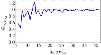
Figure 6: Dependence of the figure of merit $\Theta_{{\cal C}_{1}{\cal C}_{2a}}$ on the cycle wavelength, $\lambda_{0}$. The dashed lines $\Theta_{{\cal C}_{1}{\cal C}_{2a}}=1$ indicates the expected result in the perfectly adiabatic limit.

Non-adiabatic effects may limit the possibility to isolate non-abelian holonomies. Differently from geometric contributions, non-adiabatic transitions will be however sensitive to the cycle duration and they could in principle be isolated performing a study of the figure of merit as a function of $\lambda_{0}$ as illustrated in Fig.6. There we show how the figure of merit, $\Theta_{{\cal C}_{1}{\cal C}_{2a}}$ depends on the wavelength $\lambda_{0}$ the dashed line represent the asymptotic value in the adiabatic limit. The wavelength is normalized to the minimum longitudinal momentum interval $\Delta\kappa_{\rm min}$ that is the minimum difference between the momenta of the Bloch eigenmodes. Analogous methods can be used to isolate possible dispersive effects due to imperfections in the preparation of the initial state.

V conclusions

Non-abelian gauge fields lie at the very heart of many modern physical theories. We need new experimental routes and observables to disclose the importance of the Wilczek and Zee holonomy. Recently, it was shown that they lead to non-abelian Bloch oscillations and they induce a topologically protected inter-band beating.diliberto2020 We have shown that properly designed photonic lattices enable the control of the beam evolution by non-commutative fields, allowing to test experimentally a relation between non-abelian holonomies and the displacement of the photon beam. While standard Thouless pumping simply yields a displacement of the injected signal across the lattice, non-abelian Thouless pumping yields a displacement across the lattice and it generates a holonomic transformation among the different bands. Illustrating the peculiar geometrical meaning of Wannier center displacement in lattices with degenerate bands, the present work extends the known results of Resta and Vanderbilt resta2007 and hinting at the possibility to detect the signatures of Wilczek-Zee connection in solids furthermore, it points at the possibility to investigate the role of non-abelian holonomies also in quantum Hall experiments.

Non-abelian Thouless pumping can be generalized in several directions, including nonlinear effects, see for example Ref. [smirnova2020, ], or considering the propagation of non-classical light in non-abelian lattices. Both these possibilities are unexplored so far and open several new questions concerning - for example - the effect of the non-abelian holonomy on entanglement or the impact of nonlinearity in breaking the hidden symmetries. Non-abelian topological photonics may stimulate further developments and applications for classical and quantum information pinske2020 and tests of fundamental physics.

VI Acknowledgments

The present research was supported by Sapienza Ateneo, QuantERA ERA-NET Co-fund (Grant No. 731473, QUOMPLEX), PRIN PELM (20177PSCKT), the H2020 PhoQus (Grant No. 820392) and by Regione Lazio (L. R. 13/08) through project SIMAP.
Rosario Fazio acknowledges partial financial support from the Google Quantum Research Award. R. F. research has been conducted within the framework of the Trieste Institute for Theoretical Quantum Technologies (TQT).

Appendix A Spectrum of the non-abelian Lieb chain

As discussed in Section II, a suitable basis to describe the propagation of electromagnetic waves through the modulated naL chain is the local Bloch eigenmodes basis defined by the following equations

$${\cal H}_{k}(z)|\psi_{\nu\alpha}(k,z)\rangle=\kappa_{\nu}(z)|\psi_{\nu\alpha}(k,z)\rangle$$ (28)

$$\langle\psi_{\nu a}(k,z)|\psi_{\mu b}(k,z)\rangle=\delta_{\mu\nu}\delta_{ab}$$ (29)

where ${\cal H}_{k}$ is the Hamiltonian of the non-abelian Lieb chain at a given $k$

$${\cal H}_{k}=\left(\begin{array}[]{cccc}0&J_{b}(k)&J_{c}&J_{d}\\ J_{b}^{*}(k)&0&0&0\\ J_{c}&0&0&0\\ J_{d}&0&0&0\end{array}\right).$$ (30)

The set $\{|\psi_{\nu a}(k,z)\rangle\}$ yields the spectrum of the naL Hamiltonian, and it features two dispersionless degenerate modes, $|\psi_{01}\rangle$ and $|\psi_{02}\rangle$, with longitudinal momentum, $\kappa_{0}=0$, given by Eq.(6) and two dispersive modes, $|\psi_{\pm}\rangle$, defined as

$$\psi_{\pm}=\frac{1}{\sqrt{2}}\left(|a_{k}\rangle\pm\frac{J_{b}(k)|b_{k}\rangle+J_{c}|c_{k}\rangle+J_{d}|d_{k}\rangle}{\Delta(k)}\right)$$ (31)

with longitudinal momenta $\kappa_{\pm}=\pm\Delta(k)$ where $\Delta(k)=\sqrt{J^{2}_{b}(k)+J_{c}^{2}+J_{d}^{2}}$ and $J_{b}(k)=J_{b1}+J_{b2}e^{ik}$. In the above equations $|m_{k}\rangle$ are the standard Bloch vectors, $|m_{k}\rangle=\sum_{i}|m_{i}\rangle e^{ikR_{i}}$ with $m=a,b,c,d$ and $|m_{i}\rangle$ indicating a state localized on the site $m$ of the cell $i$ located at $x=R_{i}$.

Appendix B Non-commutative nature of the displacement generated in composite cycles

As shown in Section III, starting from specific examples, the non-abelian nature of the evolution implies that, when we perform a sequence of two cycles, the displacement depends on the ordering of the sequence. To understand this fact, let us take two generic cycles, ${\cal C}_{x}$ and ${\cal C}_{y}$, and the two possible sequences of the two, namely, ${\cal C}_{x}{\cal C}_{y}$ and ${\cal C}_{y}{\cal C}_{x}$. In the latter case, i.e. if we cover first the cycle ${\cal C}_{x}$ and then the cycle ${\cal C}_{y}$, the displacement matrix reads

$$\left[D_{{\cal C}_{x}{\cal C}_{y}}\right]_{ab}=\left[D_{{\cal C}_{y}}\right]_{ab}+\frac{1}{2\pi}\int dk\left[W^{{\dagger}}_{{\cal C}_{y}}{\hat{D}}_{{\cal C}_{x}}W_{{\cal C}_{y}}\right]_{ab}$$ (32)

while in the opposite case it reads

$$\left[D_{{\cal C}_{y}{\cal C}_{x}}\right]_{ab}=\left[D_{{\cal C}_{x}}\right]_{ab}+\frac{1}{2\pi}\int dk\left[W^{{\dagger}}_{{\cal C}_{x}}{\hat{D}}_{{\cal C}_{y}}W_{{\cal C}_{x}}\right]_{ab}$$ (33)

where $W_{\cal C}$ and ${D}_{{\cal C}}$ indicate respectively the holonomy and the displacement matrix of the cycle ${\cal C}$ while ${\hat{D}}_{{\cal C}}$ denotes the $k$-dependent displacement matrix of the cycle ${\cal C}$, i.e. ${\hat{D}}_{{\cal C}}=\oint_{{\cal C}}W^{{\dagger}}{\cal F}W\,dz$. From the above equations we see that two cycles performed in different orders generate in general different displacements, due to the non-commutativity of $W_{\cal C}$ and ${\hat{D}}_{{\cal C}}$.

This fact is true in particular for the cycles ${\cal C}_{1}$ and ${\cal C}_{2a}$ or ${\cal C}_{2b}$ presented in Section III. We notice that, independently on the initial state the displacement accumulated along the cycles ${\cal C}_{2a}$ or ${\cal C}_{2b}$ is zero, since along these cycles the coupling $J_{b1}$ vanishes, i.e. we have

$$D_{{\cal C}_{2a}}=D_{{\cal C}_{2b}}=0$$ (34)

Substituting the previous relations in Eqs.(32-33) we obtain the following result for the photon displacement for the composite cycles ${\cal C}_{2i}{\cal C}_{1}$ and ${\cal C}_{1}{\cal C}_{2i}$

$$D_{{\cal C}_{2i}{\cal C}_{1}}=D_{{\cal C}_{1}}$$ (35)

and

$$D_{{\cal C}_{1}{\cal C}_{2i}}=\frac{1}{2\pi}\int dk\left[W^{{\dagger}}_{{\cal C}_{2i}}{\hat{D}}_{{\cal C}_{1}}W_{{\cal C}_{2i}}\right]$$ (36)

with $i=a\,{\rm or}\,b$.

Appendix C Holonomies, field-strength and displacement of the cycles of ${\cal C}_{1}$, ${\cal C}_{2a}$ and ${\cal C}_{2b}$

In this Appendix we relate the holonomies and displacements generated in the cycles ${\cal C}_{1}$, ${\cal C}_{2a}$ and ${\cal C}_{2b}$ to the geometrical structure of these cycles. Most numerical results presented in Section III will be explained analytically.

We start by estimating the holonomies, $W_{{\cal C}_{1}}$, $W_{{\cal C}_{2i}}$ with $i=a,\,b$. The general expression of the connection matrix, $\Gamma^{z}_{0}$, assuming a generic dependence of all tunnel coupling $J_{i}$ on $z$, is

$$\Gamma^{z}_{0} = \frac{\left(J_{b2}\partial_{z}{J}_{b1}-J_{b1}\partial_{z}{J}_{b2}\right)\sin k}{\Delta^{2}(k)}\left(\begin{array}[]{cc}0&0\\ 0&1\\ \end{array}\right)+$$ (42)

$$+\frac{\left(J_{c}\partial_{z}J_{d}-J_{d}\partial_{z}J_{c}\right)|J_{b}|}{\delta^{2}\Delta(k)}\left(\begin{array}[]{cc}0&ie^{i\phi_{k}}\\ -ie^{-i\phi_{k}}&0\\ \end{array}\right),$$

where we set $\phi_{k}=\arg(J_{b1}+J_{b2}e^{ik})$ The connection along $k$ is instead given by

$$\Gamma_{0}^{k} = -\frac{J_{b2}\left(J_{b2}+J_{b1}\cos k\right)}{\Delta^{2}(k)}\left(\begin{array}[]{cc}0&0\\ 0&1\\ \end{array}\right).$$ (46)

From the above equations we can easily evaluate the holonomies of the cycles ${\cal C}_{1}$ and ${\cal C}_{2i}$ with $i=a,b$, we obtain

$$W_{{\cal C}_{1}} = \exp\left[i\Delta_{{\cal C}_{1}}\frac{1}{2}\left(\sigma_{0}-\sigma_{z}\right)\right]$$ (47)

$$W_{{\cal C}_{2i}} = \exp\left[i\Delta_{{\cal C}_{2i}}\left(\sin(k)\sigma_{x}+\cos(k)\sigma_{y}\right)\right]$$ (48)

with $\sigma_{0}$ denoting the $2\times 2$ identity matrix and $\sigma_{x},\,\sigma_{y}$ and $\sigma_{z}$ the three standard Pauli matrices. To derive equations (47-48), we used the fact that, along the paths ${\cal C}_{2i}$, $J_{b2}$ is constant and $J_{b1}=0$ and we indicated with $\Delta_{{\cal C}_{1}}$ and $\Delta_{{\cal C}_{2i}}$ the following integrals

$$\Delta_{{\cal C}_{1}}=\oint_{{\cal C}_{1}}\frac{\left(J_{b1}\partial_{z}{J}_{b2}-J_{b2}\partial_{z}{J}_{b1}\right)\sin k}{J_{d}^{2}+J_{c}^{2}+|J_{b}|^{2}},$$ (49)

$$\Delta_{{\cal C}_{2i}}=\oint_{{\cal C}_{2i}}\frac{\left(J_{c}\partial_{z}J_{d}-J_{d}\partial_{z}J_{c}\right)J_{b2}}{(J_{c}^{2}+J_{d}^{2})(J_{c}^{2}+J_{d}^{2}+J_{b2}^{2})^{1/2}}.$$ (50)

Both integrals can be easily calculated and they have a simple geometrical meaning.

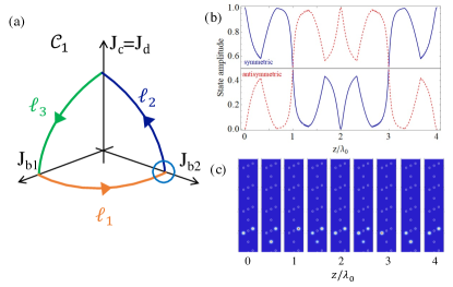
Figure 7: (a) Structure of the cycle ${\cal C}_{1}$. (b) Evolution of the occupation of the two Bloch eigenmodes along the cycle ${\cal C}_{2a}$, the solid and dotted lines correspond respectively to the states $|\psi_{02}\rangle$ and $|\psi_{01}\rangle$. (c) Density plots of the field intensity across the lattice at different $z$ along the cycle ${\cal C}_{2a}$.

Specifically, for $\Delta_{{\cal C}_{1}}$ we have:

$$\Delta_{{\cal C}_{1}}=\int_{\ell_{1}}\partial_{z}\arg\phi_{k}=k$$ (51)

where $\ell_{1}$ denotes the portion of the curve ${{\cal C}_{1}}$ laying on the $J_{b1},J_{b2}$ plane, see Fig. 7(a).

Along the cycle ${\cal C}_{1}$ the occupation of the two eigenstates does not change however, the structure of the state $\psi_{02}$ is deformed in such a way that its Wannier center is displaced by one unit cell per cycle as one can clearly see in Figs.2(a) and 3(a).

At variance with $\Delta_{{\cal C}_{1}}$, the integral $\Delta_{{\cal C}_{2i}}$ depends on the precise shape of the cycle. For the two examples shown in Fig.2(b) of the main text the calculation is straightforward; specifically, we get $\Delta_{{\cal C}_{2i}}=\pi/2-\alpha_{i}$ with $\alpha_{a}=\pi/4$ and $\alpha_{b}=\pi/3$ where the $\pi/2$ contribution comes in both cases from the fact that we assume an infinitesimal value of $J_{c}=J_{d}$ at the starting point to avoid ambiguities in the definition of the states. We notice that $\Delta_{{\cal C}_{2i}}$ has a simple geometric interpretation, indeed, denoting with $\bar{\cal C}_{2i}$ the projection of the path ${\cal C}_{2i}$ on the unitary sphere in the space $J_{c}$,$J_{d}$, $J_{b2}$, one can show that $\Delta_{{\cal C}_{2i}}$ yields the solid angle subtended by the path $\bar{\cal C}_{2i}$ at the origin.
To see this we introduce the cartesian coordinates $\{x,y,z\}=\{J_{c},J_{d},J_{b2}\}$ and we rewrite $\Delta_{{\cal C}_{2i}}$ as:

$$\Delta_{{\cal C}_{2i}}=\int_{{\cal C}_{2i}}\frac{z\left(ydx-x\,dy\right)}{(x^{2}+y^{2})\sqrt{x^{2}+y^{2}+z^{2}}}.$$ (52)

Noting that

$$\nabla\times\left[\frac{z\left(-y,x,0\right)}{(x^{2}+y^{2})\sqrt{x^{2}+y^{2}+z^{2}}}\right]=\frac{(x,y,z)}{\left(x^{2}+y^{2}+z^{2}\right)^{\frac{3}{2}}}$$

and applying Stokes theorem we can then rewrite the contour integral in Eq.(52) as a surface integral as follows

$$\Delta_{{\cal C}_{2i}}=\int_{\Sigma_{i}}\frac{\vec{r}}{r^{3}}\cdot d\vec{\sigma}$$ (53)

where we denoted with $\vec{r}$ the vector $\left(x,y,z\right)$ and with $\Sigma_{i}$ a surface such that $\partial\Sigma_{i}={\cal C}_{2i}$. Eventually, indicating as $\bar{\Sigma}_{i}$ the portion of the unitary sphere,$S^{2}$, enclosed by $\bar{\cal C}_{2i}$, with an appropriate choice of $\Sigma_{i}$ we can easily obtain the desired result, i.e.

$$\Delta_{{\cal C}_{2i}}=\int_{\bar{\Sigma}_{i}}\frac{\vec{r}}{r^{3}}\cdot d\vec{\sigma}=\int_{\bar{\Sigma}_{i}}d\omega$$ (54)

where we have used the fact that, on $S^{2}$, $d\vec{\sigma}=d\omega\hat{r}$ with $d\omega$ the differential of solid angle. In Figure 7(b) we show the evolution of the population of the two eigenstates along the cycle ${\cal C}_{2a}$ , as one can see this cycle yields a rotation by $3\pi/4$.

We now focus on the displacement matrices. To this end, we employ Eq.(14), that relates the displacement matrix to the field strength. We thus start from the following general expression of the field strength matrix, ${\cal F}$,

$${\cal F}_{zk}=\frac{\left(J_{c}\partial_{z}J_{d}-J_{d}\partial_{z}J_{c}\right)J_{b2}}{\Delta^{3}(k)}\left(\begin{array}[]{cc}0&e^{ik}\\ e^{-ik}&0\\ \end{array}\right)+\frac{J_{b2}\left[(J_{b2}+J_{b1}\cos(k))\partial_{z}\delta^{2}-\delta^{2}\partial_{z}(J_{b2}+J_{b1}\cos(k))\right]}{\Delta^{4}(k)}\left(\begin{array}[]{cc}0&0\\ 0&1\\ \end{array}\right).$$ (55)

where we assumed that all tunnel couplings are generic function of $z$.

Analogously to Eqs.(42-46), Eq.(55) substantially simplifies if we consider the geometrical structure of the cycles.

Along the cycle ${\cal C}_{1}$ we have $J_{c}=J_{d}$, the first term in Eq.(55) is thus vanishing and the field strength ${\cal F}$ can be cast as

$${\cal F}_{zk}\xrightarrow[\text{along ${\cal C}_{1}$}]{\text{{ }}}\frac{2J_{b2}J_{c}(J_{b2}\partial_{z}J_{c}-J_{c}\partial_{z}J_{b2})}{J_{b2}^{2}+J_{c}^{2}}\left(\begin{array}[]{cc}0&0\\ 0&1\\ \end{array}\right)$$ (56)

This term is non-vanishing only along the portion $\ell_{2}$ of the cycle ${\cal C}_{1}$, it does not depend on $k$ and it commutes with the holonomy $W_{{\cal C}_{1}}$. Furthermore, as one can easily check, integrated over $z$ and $k$ yields $2\pi$. It thus leads to the following expression for the displacement matrix of the cycle ${\cal C}_{1}$

$$D_{{\cal C}_{1}}=\left(\begin{array}[]{cc}0&0\\ 0&1\\ \end{array}\right).$$ (57)

As explained above, the displacement generated along the cycles ${\cal C}_{2i}$ is zero nevertheless, by looking at equation (55) we notice that along these cycles we have a finite field strength. As one can explicitly verify, the zero displacement results is indeed recovered after integrating over $k$ and $z$. In these regards we note that for $J_{b2}=0$ the field strength is identically zero, opposite to what happens for $J_{b1}=0$, Since, due to the lattice periodicity I can always exchange the roles of $J_{b1}$ and $J_{b2}$ and I expect that the symmetry between the two cases is restored upon averaging over $k$, this is indeed the case.

A possible route to demonstrate the non-commutative nature of non-abelian Thouless pumping is to design a pumping cycle aimed at detecting the contribution to the displacement of the commutator term ${\cal F}^{\rm com}_{zk}=i\left[\Gamma_{z},\Gamma_{k}\right]$, peculiar of non-abelian gauge theories. We remark that, in spite of the apparent complexity, in Eq. (42) we have a cancellation between terms coming from the abelian contribution to the field strength, $\partial_{k}\Gamma^{z}_{\nu}-\partial_{z}\Gamma^{k}_{\nu}$ and from the non-abelian commutator, ${\cal F}^{\rm com}_{zk}$. It is interesting to look at the explicit expression of the latter

$${\cal F}^{\rm com}_{zk} = \frac{\left(J_{c}\partial_{z}J_{d}-J_{d}\partial_{z}J_{c}\right)|J_{b}|J_{b2}(J_{b2}+J_{b1}\cos(k))}{\delta^{2}\Delta^{3}(k)}\cdot$$ (60)

$$\cdot\left(\begin{array}[]{cc}0&ie^{i\phi_{k}}\\ -ie^{-i\phi_{k}}&0\\ \end{array}\right),$$

by looking at the above equation we see that if $J_{b1}$ or $J_{b2}$ are identically zero along the cycle the contribution of this terms vanishes upon averaging over $k$. To see the contribution of this term in pumping we thus need to design a cycle having all the coupling different from zero at some point.

Appendix D Non-commuting cycles sequences

Using the above results, the holonomies for the composite cycles ${\cal C}_{1}{\cal C}_{2}$ and ${\cal C}_{2}{\cal C}_{1}$ can be explicitly calculated. They are given by

$$W_{{\cal C}_{1}{\cal C}_{2}}=\left(\begin{array}[]{cc}\cos(\Delta_{{\cal C}_{2}})&e^{ik}\sin(\Delta_{{\cal C}_{2}})\\ -\sin(\Delta_{{\cal C}_{2}})&e^{ik}\cos(\Delta_{{\cal C}_{2}})\\ \end{array}\right)$$ (61)

and

$$W_{{\cal C}_{2}{\cal C}_{1}}=\left(\begin{array}[]{cc}\cos(\Delta_{{\cal C}_{2}})&e^{2ik}\sin(\Delta_{{\cal C}_{2}})\\ -e^{-ik}\sin(\Delta_{{\cal C}_{2}})&e^{ik}\cos(\Delta_{{\cal C}_{2}})\\ \end{array}\right)$$ (62)

The corresponding displacement matrices can be instead expressed as follows:

$$D_{{\cal C}_{2}{\cal C}_{1}} = D_{{\cal C}_{1}}=\left(\begin{array}[]{cc}0&0\\ 0&1\\ \end{array}\right)$$ (65)

$$D_{{\cal C}_{1}{\cal C}_{2}} = \left(\begin{array}[]{cc}\sin^{2}\Delta_{{\cal C}_{2}}&0\\ 0&\cos^{2}{\Delta_{{\cal C}_{2}}}\\ \end{array}\right)$$ (68)

Equations (61-62) ashow that the holonomy transformations for the cycles ${\cal C}_{1}$ and ${\cal C}_{2}$ do not commute, i.e. starting from a given initial state, the final state and the displacement obtained depend on wether we perform first the cycle ${\cal C}_{1}$ and then the cycle ${\cal C}_{2}$ or viceversa. In the table below we explicitly calculate the final state and displacement generated starting from different localized initial states. Specifically, we consider the case where the initial states are simply $|c_{n}\rangle$ and $|d_{n}\rangle$, and get:

Cycles Initial state Final state Displacement

$${\cal C}_{2}{\cal C}_{1}$$

(69)

with $2\eta_{\pm}=\cos(\Delta_{{\cal C}_{2}})\pm\sin(\Delta_{{\cal C}_{2}})$.

References

- (1) R. Bott and S. S. Chern, Acta Mathematica 114, 71 (1965).
- (2) B. Simon, Phys. Rev. Lett. 51, 2167 (1983).
- (3) M. V. Berry, Proceedings of the Royal Society of London. A. Mathematical and Physical Sciences 392, 45 (1984).
- (4) F. Wilczek and A. Zee, Phys. Rev. Lett. 52, 2111 (1984).
- (5) F. Wilczek and A. Shapere, Geometric Phases in Physics, World Scientific, Singapore, 1989.
- (6) R. Resta and D. Vanderbilt, in Physics of Ferroelectrics, edited by K. M. Rabe, C. H. Ahn, and J.-M. Triscone (Springer-Verlag GmbH, Berlin, 2007), Chap. Theory of Polarization: A Modern Approach.
- (7) D. J. Thouless, M. Kohmoto, M. P. Nightingale, and M. den Nijs, Phys. Rev. Lett. 49, 405 (1982).
- (8) D. J. Thouless, Phys. Rev. B 27, 6083 (1983).
- (9) M. Aunola and J. J. Toppari, Phys. Rev. B 68, 020502 (2003).
- (10) M. Möttönen, J. P. Pekola, J. J. Vartiainen, V. Brosco, and F. W. J. Hekking, Phys. Rev. B 73, 214523 (2006).
- (11) D. Xiao, M.-C. Chang, and Q. Niu, Rev. Mod. Phys. 82, 1959 (2010).
- (12) O. Zilberberg, S. Huang, J. Guglielmon, M. Wang, K. P. Chen, Y. E. Kraus, and M. C. Rechtsman, Nature 553, 59 (2018).
- (13) H. M. Price, O. Zilberberg, T. Ozawa, I. Carusotto, and N. Goldman, Phys. Rev. B 93, 245113 (2016).
- (14) M. Aidelsburger, M. Lohse, C. Schweizer, M. Atala, J. T. Barreiro, S. Nascimbène, N. R. Cooper, I. Bloch, and N. Goldman, Nature Physics 11, 162 (2014).
- (15) Y. E. Kraus, Y. Lahini, Z. Ringel, M. Verbin, and O. Zilberberg, Phys. Rev. Lett. 109, 106402 (2012).
- (16) Y. Ke, X. Qin, F. Mei, H. Zhong, Y. S. Kivshar, and C. Lee, Laser & Photonics Reviews 10, 1064 (2016).
- (17) M. Wimmer, H. M. Price, I. Carusotto, and U. Peschel, Nat. Phys. 13, 545 (2017).
- (18) Z. Fedorova, C. Jörg, C. Dauer, F. Letscher, M. Fleischhauer, S. Eggert, S. Linden, and G. von Freymann, Light: Science & Applications 8, 63 (2019).
- (19) Y. Wang, Y.-H. Lu, F. Mei, J. Gao, Z.-M. Li, H. Tang, S.-L. Zhu, S. Jia, and X.-M. Jin, Phys. Rev. Lett. 122, 193903 (2019).
- (20) M. Lohse, C. Schweizer, O. Zilberberg, M. Aidelsburger, and I. Bloch, Nat. Phys. 12, 350 (2015).
- (21) S. Nakajima, T. Tomita, S. Taie, T. Ichinose, H. Ozawa, L. Wang, M. Troyer, and Y. Takahashi, Nat. Phys. 12, 296 (2016).
- (22) M. Kremer, I. Petrides, E. Meyer, M. Heinrich, O. Zilberberg, and A. Szameit, Nature Communications 11, 907 (2020).
- (23) E. H. Lieb, Phys. Rev. Lett. 62, 1201 (1989).
- (24) R. A. Vicencio, C. Cantillano, L. Morales-Inostroza, B. Real, C. Mejía-Cortés, S. Weimann, A. Szameit, and M. I. Molina, Phys. Rev. Lett. 114, 245503 (2015).
- (25) S. Mukherjee, A. Spracklen, D. Choudhury, N. Goldman, P. Öhberg, E. Andersson, and R. R. Thomson, Phys. Rev. Lett. 114, 245504 (2015).
- (26) L.-M. Duan, Science 292, 1695 (2001).
- (27) L. Taddia, E. Cornfeld, D. Rossini, L. Mazza, E. Sela, and R. Fazio, Phys. Rev. Lett. 118, 230402 (2017).
- (28) L. Faoro, J. Siewert, and R. Fazio, Phys. Rev. Lett. 90, 028301 (2003).
- (29) V. Brosco, R. Fazio, F. W. J. Hekking, and A. Joye, Phys. Rev. Lett. 100, 027002 (2008).
- (30) J. Pachos and S. Chountasis, Phys. Rev. A 62, 052318 (2000).
- (31) T. Iadecola, T. Schuster, and C. Chamon, Phys. Rev. Lett. 117, 073901 (2016).
- (32) Y. Chen, R.-Y. Zhang, Z. Xiong, Z. H. Hang, J. Li, J. Q. Shen, and C. T. Chan, Nat. Commun. 10, 1 (2019).
- (33) J. W. Zwanziger, M. Koenig, and A. Pines, Phys. Rev. A 42, 3107 (1990).
- (34) J. M. Martinis, M. H. Devoret, and J. Clarke, Nat. Phys. 16, 234 (2020).
- (35) A. A. Abdumalikov, J. M. Fink, K. Juliusson, M. Pechal, S. Berger, A. Wallraff, and S. Filipp, Nature 496, 482 (2013).
- (36) T. Ozawa, H. M. Price, A. Amo, N. Goldman, M. Hafezi, L. Lu, M. C. Rechtsman, D. Schuster, J. Simon, O. Zilberberg, and I. Carusotto, Rev. Mod. Phys. 91, 015006 (2019).
- (37) D. N. Christodoulides, F. Lederer, and Y. Silberberg, Nature 424, 817 (2003).
- (38) A. W. Snyder and J. Love, Optical Waveguide theory, Springer, Berlin, 1983.
- (39) M. Kremer, L. Teuber, A. Szameit, and S. Scheel, Phys. Rev. Research 1, 033117 (2019).
- (40) W. Casteels, R. Rota, F. Storme, and C. Ciuti, Phys. Rev. A 93, 043833 (2016).
- (41) M. Biondi, G. Blatter, and S. Schmidt, Phys. Rev. B 98, 104204 (2018).
- (42) Coherently with the quantum interpretation of the classical Maxwell equations we use a bra-ket notation.
- (43) J. Zak, Physical Review Letters 62, 2747 (1989).
- (44) P. M. Fishbane, S. Gasiorowicz, and P. Kaus, Phys. Rev. D 24, 2324 (1981).
- (45) N. Manton and P. Sutcliffe, Topological Solitons (Cambridge University Press, Cambridge, UK, 2004).
- (46) D. Smirnova, D. Leykam, Y. Chong, and Y. Kivshar, Appl. Phys. Rev. 7, 021306 (2020).
- (47) Q. Chen, J. Cai and S. Zhang, Phys. Rev. A 101, 043614 (2020)
- (48) A. Cerjan, M. Wang, S. Huang, et al. Light. Sci. Appl. 9, 178 (2020).
- (49) A. Yariv, IEEE J. Quantum Electron., 9, 919 (1973).
- (50) A. Snyder, J. Opt. SOC. Amer., 62, 1267 (1972).
- (51) D. Marcuse, Bell. Sys. Tech. J. 52, 817 (1973)
- (52) J. Pinske and S. Scheel arXiv:2105.04859 (2021).
- (53) B. M. Rodriguez-Lara, Francisco Soto-Eguibar, Demetrios N. Christodoulides, Phys. Scr. 90, 068014 (2015)
- (54) M. Di Liberto, N. Goldman and G. Palumbo, Nature Communications 11, 5942 (2020)
- (55) J. Pinske, L. Teuber, and S. Scheel, Phys. Rev. A 101, 062314 (2020)