Panoster: End-to-end Panoptic
Segmentation of LiDAR Point Clouds

Abstract

Panoptic segmentation has recently unified semantic and instance segmentation, previously addressed separately, thus taking a step further towards creating more comprehensive and efficient perception systems. In this paper, we present Panoster, a novel proposal-free panoptic segmentation method for LiDAR point clouds. Unlike previous approaches relying on several steps to group pixels or points into objects, Panoster proposes a simplified framework incorporating a learning-based clustering solution to identify instances. At inference time, this acts as a class-agnostic segmentation, allowing Panoster to be fast, while outperforming prior methods in terms of accuracy. Without any post-processing, Panoster reached state-of-the-art results among published approaches on the challenging SemanticKITTI benchmark, and further increased its lead by exploiting heuristic techniques. Additionally, we showcase how our method can be flexibly and effectively applied on diverse existing semantic architectures to deliver panoptic predictions.

I Introduction

Scene understanding is a fundamental task for autonomous vehicles. Panoptic segmentation (PS) [1] combines semantic and instance segmentation, enabling a single system to develop a more complete interpretation of its surroundings. PS distinguishes between stuff and thing classes [1], with the former being uncountable and amorphous regions, such as road and vegetation, and the latter standing for countable objects, such as people and cars. The two have been addressed separately for decades, leading to significantly different approaches: stuff classifiers are typically based on fully convolutional networks [2], while thing detectors often rely on region proposals and the regression of bounding-boxes [3]. Tackling semantic and instance segmentation jointly with PS allows to save costly and limited resources [4].

Since the introduction of PS, several approaches have been proposed to address this new task. While most focused on images [5, 4, 6] or RGBD data [7, 8], only a handful of methods used LiDAR point clouds [9, 10], none of which has managed to outperform systems combining separate networks for semantic segmentation and object detection [11]. LiDAR sensors have proven to be particularly useful for self-driving cars, capturing precise distance measurements of the surrounding environment. Segmenting LiDAR point clouds is a crucial step for interpreting the scene. Compared to image pixels, LiDAR point clouds pose various challenges: they are unstructured, unordered, sparse, and irregularly sampled.

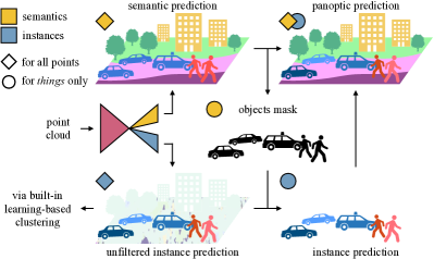
Figure 1: Proposed Panoster framework. A semantic class and an instance ID are predicted for every point, then filtered and combined for panoptic segmentation.

In this paper, we introduce a novel proposal-free approach for panoptic segmentation of LiDAR point clouds. We name our method Panoster, standing for panoptic clustering. Panoster brings panoptic capabilities to semantic segmentation networks by adding an instance branch trained to resolve objects with a learning-based clustering method adapted from [12]. Unlike existing proposal-free approaches [6, 10], Panoster, thanks to its clustering solution integrated in the model, does not need further groupings to form objects, as it outputs instance IDs straight away from the network. The contributions of this paper can be summarized as follows:

• We introduce a new proposal-free approach for panoptic segmentation, fully end-to-end, flexible and fast, with a small overhead on top of an equivalent semantic segmentation architecture.

• To the best of our knowledge, for the first time in panoptic segmentation, we exploit an entirely learning-based end-to-end clustering approach to separate the instances, resulting in a fully end-to-end panoptic method.

• Our novel instance segmentation acts as class-agnostic segmentation, has no thresholds, and delivers instance IDs directly, without requiring further grouping steps.

We apply Panoster on the challenging task of panoptic segmentation for LiDAR 3D point clouds, outperforming in a fraction of the time state-of-the-art methods. Furthermore, we show the flexibility of Panoster by deploying it on both projection-based and point-based architectures, making it the first panoptic method to consume LiDAR 3D points directly.

II Related Work

In this section, we provide a brief overview of existing approaches, and highlight overlaps and differences with Panoster.

II-A Semantic Segmentation

Depending on the input representation, semantic segmentation methods can be grouped into projection-based and point-based. Projection-based approaches eliminate the challenging irregularities of 3D points by projecting them into an intermediate grid. This grid representation can be made of voxels [13, 14] or pixels [15, 16], allowing the use of 3D or 2D convolutions respectively. While the former projection tends to be highly inefficient for this task, the latter can count on state-of-the-art methods from image segmentation, albeit discarding valuable geometric information by transitioning from 3D to 2D.

PointNet [17] pioneered point-based methods and deep learning on point clouds. They used multilayer perceptrons (MLP) to learn features from each point, then aggregated with a global max-pooling. Additional MLP-based architectures were proposed in [18, 19, 20]. More recent approaches, such as KPConv [21] and SpiderCNN [22] have focused on creating new convolution operations for points. KPConv [21] extended the idea of 2D image kernels to 3D points, by defining an operation which derives new 3D points from the multiplication of input 3D point features with flexible kernel weights. Recently, hybrid approaches have been developed [23, 24], combining point and projection-based solutions.

Our method Panoster extends semantic segmentation approaches to panoptic segmentation. In this paper we apply Panoster on KPConv [21] and SalsaNext [16], representative of point-based and projection-based categories respectively.

II-B Instance Segmentation

Instance segmentation methods can be divided into detection-based and clustering-based. The former was established in the image domain by Mask R-CNN [25] which has two stages: region proposals are extracted, refined into bounding boxes, and segmented with a pixel-level mask to identify the objects. Mask R-CNN has catalyzed a variety of methods, some of which address panoptic segmentation [4, 26, 9], as described in Section II-C. Clustering-based approaches learn an embedding space in which instances can be easily clustered [27, 28]. Therefore, the segmentation is typically done by deploying a data analysis clustering technique, such as DBSCAN [29], on the latent features, which were learned to aid the separation. These methods were extended to point clouds in [30, 31, 32].

Panoster operates differently, by clustering object instances thanks to loss functions optimizing the network outputs directly. Although our instance segmentation is learning-based, it does not explicitly rely on the optimization of a latent space via embeddings, differentiating itself from clustering-based methods described above. Furthermore, Panoster performs panoptic segmentation, resulting in a more comprehensive approach.

II-C Panoptic Segmentation

PS methods can be divided into two categories: proposal-based and proposal-free. The vast majority are from the image domain, of which the larger stake are proposal-based or top-down methods (e.g. UPSNet [26], AdaptIS [33], Seamless [5], EfficientPS [4]): two-stage approaches, which are usually based on the well-known Mask R-CNN [25]. They rely on the detection of things first, followed by a refinement step and a semantic segmentation of stuff. Their main drawbacks are the needs of resolving mask overlaps and conflicts between thing and stuff predictions. Instead, proposal-free or bottom-up methods are single-stage and follow the opposite direction. They segment the scene semantically, and cluster the instances within the predicted thing segments. DeeperLab [34] was the first of this kind, regressing objects center and corners from images. SSAP [35] used a cascaded graph partition module to group pixels into instances according to a pixel-pair affinity pyramid. Panoptic-DeepLab [6] simplified this concept by predicting the instance center locations, and using a Hough-Voting scheme to group the pixels to the closest center.

While PS received a lot of attention in the image domain, PS on LiDAR point clouds is yet broadly unexplored, due to the only recent introduction of a suitable public dataset, i.e. SemanticKITTI with panoptic labels [11]. In [11] strong baselines combined state-of-the-art semantic segmentation methods KPConv [21] or RangeNet++ [15], with the object detector PointPillars [20]. PanopticTrackNet [9] followed the approach of EfficientPS [4] and extended it to consume LiDAR point clouds: it is top-down, based on Mask R-CNN [25] to resolve the instances. Additionally, a new tracking head delivers temporally consistent instance IDs. The only existing bottom-up method for LiDAR point clouds is [10], which we denote as LPSAD. It is based on semantic embeddings and, as in Panoptic-DeepLab [6], the regression of offsets to the object centers, then instances are extracted by an iterative clustering procedure, grouping points according to their center offset prediction. To date, no method managed to outperform the combined baselines proposed in [11].

Panoster is significantly different from existing panoptic approaches. It is the first to use an entirely learning-based clustering technique to resolve the instances. As LPSAD [10], our method is bottom-up and applied on LiDAR point clouds, but compared to it, our instance branch outputs instance IDs directly, without requiring any subsequent grouping steps, rendering it fully end-to-end trainable.

III Panoster

III-A Overview

As described in Section II-C, current proposal-free panoptic approaches [6, 10] pair a network with an external grouping technique to form objects. The latter exploits the network predictions, and is required in order to output any meaningful instance IDs. With the proposed Panoster, we simplify by removing this extra step, and incorporating the clustering in the network itself. We achieve this with an entirely learning-based approach, adapted from the signal processing domain [12], to output instance IDs directly, for each point given in input (Section III-C). To obtain panoptic predictions, it is then sufficient to filter out these IDs for all stuff points (Section III-D), as shown in Fig. 1. Thanks to custom loss functions, our integrated clustering method instills grouping capabilities right in the model weights. At inference time, these layers process data in the same way as their semantic segmentation counterparts, while pursuing the rather different task of instance segmentation. In Fig. 2 we showcase Panoster general architecture, highlighting how each part is trained.

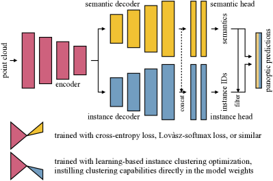
Figure 2: Panoster simplified architecture. The input is raw 3D points or a 2D spherical projection. During training, gradients do not back-propagate through the dashed line. At inference time, both decoders and heads process data in the same way.

III-B Architecture

Panoster consists of the following modules: a shared encoder, decoupled symmetric decoders and heads for the two tasks, mask-based fusion and optional post-processing.

Motivated by [6, 9, 10], we opt for a shared encoder with two separate decoders, each developing its task starting from common features. Following Fig. 2, the backbone, the semantic decoder and head follow the design of a standard semantic segmentation network, consuming a full 360 degree LiDAR point cloud. In this paper we apply Panoster on KPConv [21] and SalsaNext [16]. We refer to the two variants as PanosterK and PanosterS, respectively. Therefore, depending on the configuration, our framework can be fed with raw 3D points or with a 2D spherical projection.

As shown in Fig. 2, our method has a second decoder and head, dedicated to instance segmentation. From the architecture perspective, the two branches are identical, except for the size of the last layer: the semantic branch output size depends on the number of semantic classes, while the output of the instance branch is sized $N$, which is the number of predictable instances (Section III-C). Additionally, the input of the instance head is the concatenation of both decoders outputs. Apart from the input and output sizes of the heads, the two branches differ as each is optimized with its own loss function, which is designed to tackle its task.

We train the semantic branch to predict both stuff and thing classes. We use the same objective functions as in [16], namely weighted cross-entropy, and Lovàsz-softmax loss [36], optimizing the Jaccard index. We weight their sum 0.7 for PanosterK and 1.0 for PanosterS. Moreover, following [6], to improve the accuracy on small or distant thing objects, we triple the cross-entropy weight on instances smaller than 100 points for PanosterK. We found this to be not beneficial for PanosterS.

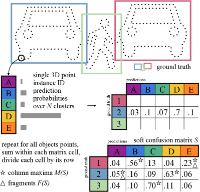
Figure 3: Construction of the matrix used for the computation of the instance clustering loss functions. The matrix $S$ is based on the instance branch segmentation probabilities, which are the cluster assignment probabilities. The figure shows a simplified scene with 3 instances and a model with $N=5$. Fragments $F(S)$ and all non-column maxima cells $Q(S)$ are minimized by fragmentation and impurity losses respectively.

III-C Learning-based Instance Clustering

Our instance branch predicts an instance ID for each point, including those belonging to stuff regions, for which such ID has no meaning and will be later filtered out (Section III-D). This instance ID is the output of the network after an argmax operation over the instance branch logits. We address instance segmentation as a class-agnostic segmentation task, with the underlying classification based on instance IDs, instead of the usual semantic classes. However, these IDs are interchangeable, similarly to clusters labels, since the essence of instance segmentation is grouping inputs to resemble object instances, e.g. instance clustering. In this Section we describe how to predict such IDs.

Towards this end, we adapt a method originally proposed for separating pulses of radar signals by source, for aircraft applications [12]. In our LiDAR panoptic task, cluster elements are 3D points, and each ground truth cluster is an object instance, e.g. a car. The idea is achieving instance segmentation by guiding the training optimization to minimize two complementary loss functions, which are extracted from a confusion matrix. However, since confusion matrices are inherently non-differentiable, being based on argmax operations over the class logits, we construct suitable matrices by considering the probability distribution over the logits softmax instead. In particular, as depicted in Fig. 3, we build this soft confusion matrix $S$ by collecting the instance branch softmax probabilities over the $N$ predictable instances, for all 3D points belonging to ground truth objects, and summing these probabilities together as follows.

For each LiDAR sweep, the softmax-based confusion matrix $S$ is sized $G\times N$, with $G$ being the number of ground truth objects. As shown in Fig. 3, the matrix $S$ gathers the instance predictions made by the network over the input 3D points. The notation in this Section refers to sets of cells, rows and columns of the matrix $S$, rather than single 3D input points. The row $S_{i}$ corresponds to the $i$-th object, while the column $S^{j}$ represents the $j$-th predicted cluster. The cell $S_{i}^{j}$ value is the sum over the probability of each point of the $i$-th object to belong to the $j$-th predicted instance, divided by the sum of the row $S_{i}$ (i.e. the amount of 3D points constituting object $i$). Unlike in [12], where the matrix values are unbounded and depend on the clusters dimensions, we introduce this division transforming the matrix in percentage-based, to render Panoster robust against the imbalance of instance sizes. The construction of $S$ is shown in Fig. 3.

This matrix $S$ is fully differentiable and can drive the network optimization. We deploy two loss functions computed from the matrix $S$, namely impurity and fragmentation. As shown in Fig. 4, by aiming at both pure and non-fragmented instances, we can achieve the best outcome.

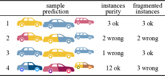
Figure 4: Sample instance segmentation predictions. In each row, colors represent predicted clusters for 3 cars. Apart for 1, 2-4 show sub-optimal results: in 2 objects are mixed and split in parts; in 3 the number of cars was underestimated, with impurity on the blue cluster, which merges two instances; in 4 the number of cars was overestimated, with severe fragmentation, as each object is split in four parts.

The impurity loss $L_{imp}$ in Eq. 1 tries to shift from 2 and 3 to 1 and 4 in Fig. 4, by optimizing instances purity:

$$\begin{matrix}L_{imp}=\frac{\sum Q(S)}{\sum S}\\ \scriptstyle Q(S):=\scriptstyle\left\{S_{i}^{j}\right\}:\>S_{i}^{j}\notin M^{j}(S)\>\>\forall i,j\end{matrix}$$ (1)

where $M(S):=\left\{\max\left(S^{j}\right)\forall~{}j\right\}$ is the set of column maxima of $S$, and $Q(S)$ is the set of all $S$ cells that are not part of $M(S)$. Column maxima $M(S)$ define each predicted instance by linking it with a ground truth object. By minimizing $Q(S)$, this loss increases the correspondence between ideal and predicted instances.

The additional fragmentation loss $L_{fr}$ reduces fragmentation. It limits overestimating the amount of objects, by penalizing the $S$ cells responsible for fragments $F(S)$, which occur when two or more column maxima $M(S)$ fall within the same row:

$$\begin{matrix}L_{fr}=\frac{\sum F(S)\,\oslash\,F(S)}{N}\\ \scriptstyle F(S)\,:=\,\scriptstyle\left\{S_{i}^{j}\right\}:\>S_{i}^{j}\in M_{i}(S)\;\land\;S_{i}^{j}\,\neq\,\scriptstyle\max\left(M_{i}(S)\right)\>\>\forall i,j\\ \scriptstyle M_{i}(S)\,:=\,\scriptstyle S_{i}\;\cap\;M(S)\end{matrix}$$ (2)

In the equation, the numerator is the differentiable equivalent of counting the fragments $F(S)$, thanks to the Hadamard element-wise division $\oslash$. Therefore, this loss enforces that each ground truth object corresponds to only one predicted instance, bringing use case 4 of Fig. 4 to 1.

Our instance branch is trained with a combination of $L_{imp}$ and $L_{fr}$, weighted 0.2 and 0.05 respectively.

TABLE I: Panoptic segmentation comparison on test set results of SemanticKITTI. All values in [%] with St for stuff and Th for thing.

Method	PQ	PQ†	SQ	RQ	PQTh	SQTh	RQTh	PQSt	SQSt	RQSt	mIoU
RangeNet++ [15] + PointPillars [20]	37.1	45.9	75.9	47.0	20.2	75.2	25.2	49.3	76.5	62.8	52.4
LPSAD [10]	38.0	47.0	76.5	48.2	25.6	76.8	31.8	47.1	76.2	60.1	50.9
KPConv [21] + PointPillars [20]	44.5	52.5	80.0	54.4	32.7	81.5	38.7	53.1	79.0	65.9	58.8
PanosterK [Ours]	45.6	52.8	78.1	57.0	32.4	77.1	41.6	55.1	78.8	68.2	60.4
PanosterK + post_* [Ours]	52.7	59.9	80.7	64.1	49.4	83.3	58.5	55.1	78.8	68.2	59.9

TABLE II: Detailed class-wise PQ results of SemanticKITTI test set. All values in [%].

Method	PQ	car	truck	bicycle	motorcycle	other vehicle	person	bicyclist	motorcyclist	road	sidewalk	parking	other ground	building	vegetation	trunk	terrain	fence	pole	traffic sign
RangeNet++ + PointP.	37.1	66.9	6.7	3.1	16.2	8.8	14.6	31.8	13.5	90.6	63.2	41.3	6.7	79.2	71.2	34.6	37.4	38.2	32.8	47.4
KPConv + PointP.	44.5	72.5	17.2	9.2	30.8	19.6	29.9	59.4	22.8	84.6	60.1	34.1	8.8	80.7	77.6	53.9	42.2	49.0	46.2	46.8
PanosterK	45.6	49.6	13.7	9.2	33.8	19.5	43.0	50.2	40.2	90.2	62.5	34.5	6.1	82.0	77.7	55.7	41.2	48.0	48.9	59.8
PanosterK + post_*	52.7	84.0	18.5	36.4	44.7	30.1	61.1	69.2	51.1	90.2	62.5	34.5	6.1	82.0	77.7	55.7	41.2	48.0	48.9	59.8

III-D Panoptic Segmentation

PS requires a semantic class for each point, as well as instance IDs for thing objects. Both branches output a prediction for each point of stuff and thing classes. However, instance IDs are meaningless for stuff points, and will be filtered out as follows. As shown in Fig. 1, we extract an object mask from the semantic prediction, distinguishing things from stuff points. We use this mask to discard instance predictions for stuff, and retain instance IDs for things. Finally, PS predictions are obtained by stacking semantic classes and instance IDs.

Optional post-processing. As described in Section III-C, unlike previous works [6, 10], our instance predictions do not necessarily require further grouping or post-processing. Nevertheless, we explored three different heuristic strategies, as plausibility checks, exploiting 3D information and the synergy between the two tasks. To improve detection and purity, DBSCAN [29] targets the third use case of Fig. 4. We call this strategy post_splitter: it splits instances which are too large in space w.r.t. their corresponding predicted semantic classes. Furthermore, to reduce fragmentation, post_merger can be deployed to fix the fourth use case of Fig. 4. It uses DBSCAN to cluster the 3D centers of those instances of the same semantic class, which are too close to each other. Finally, with post_cyclists, we turn bicyclists who have no bicycle nearby, but a motorbike, into motorcyclists.

IV Experiments

IV-A Experimental Setup

Dataset. We evaluate on the challenging Semantic-KITTI [37], which was recently extended [11] by providing instance IDs for all LiDAR scans of KITTI odometry [38]. It contains 23201 full 360 degree scans for training and 20351 for testing, sampled from 22 sequences from various German cities. We use training sequence 08 as validation split, following the convention. Annotations comprise point-wise labels within 50 meters radius across 22 classes, 19 of which evaluated on the test server: 11 stuff and 8 thing.

Model training. Experiments are focused mainly on PanosterK, based on KPConv [21], while showing the flexibility of Panoster by applying it also on SalsaNext [16] with PanosterS. Unless otherwise noted, we used the same training parameters as in [21] for PanosterK and [16] for PanosterS, with the addition of our instance clustering loss functions. To better fit the PS task, we used input point clouds covering the entire scene, instead of small regions as in [21]. At each training iteration, we fed PanosterK with at most 80K points. PanosterK used rigid KPConv kernels. For PanosterS we used batch size 4 and learning rate 0.001. We implemented our method in PyTorch and trained the models on a single NVIDIA Tesla V100 32GB GPU. We trained PanosterK from scratch for at least 200K iterations. PanosterS was pretrained on semantic segmentation, and fine-tuned on panoptic segmentation for 100K iterations. The PanosterK model submitted to the test server was trained on the entire training set, including the validation set.

Inference. Unlike KPConv [21], at inference time we fed the whole 50 meters radius scene in a single forward pass, without any test-time augmentation.

Evaluation metrics. We report mean IoU (mIoU) and panoptic quality (PQ) [1] to evaluate semantic and panoptic segmentation, both averaged over all classes. PQ can be seen as the multiplication of segmentation quality (SQ) and recognition quality (RQ) [1], with the former being the mIoU of matched segments and the latter representing the $F_{1}$ score, commonly adopted for object detection. Additionally, we report the alternative PQ^† [5], which ignores RQ for stuff classes. Since our main focus and contribution within PS is on instance segmentation, among the various metrics we concentrate on RQ^Th, i.e. the $F_{1}$ score for thing classes, which is more appropriate than PQ to compare instance segmentation performances.

IV-B Panoptic Segmentation

We compared Panoster with other published PS approaches for LiDAR point clouds, and submitted PanosterK to the SemanticKITTI challenge. Two strong baselines were proposed in [11] combining KPConv [21] or RangeNet++ [15] with PointPillars [20], semantic segmentation and object detection methods. Furthermore, we compared with PanopticTrackNet [9] and LPSAD [10], top-down and bottom-up approaches respectively.

Table I shows results on the test set. Overall, PanosterK delivered superior performance compared to previously published approaches. Despite obtaining worse semantics with a lower SQ, and significantly lower SQ^Th which penalized PQ^Th, PanosterK’s strengths are its finer instance segmentation abilities, shown on thing classes, resulting in a notable 2.9 increase in RQ^Th on top of state-of-the-art KPConv and PointPillars, albeit sharing the same backbone. Considering individual classes, Table II shows that PointPillars [20], which is a strong object detector, performed better than our instance clustering approach on the classes car, truck and bicyclist, while ours prevailed on person, motorcycle and motorcyclist. Nevertheless, compared to the combined approaches, our PanosterK was able to deliver a better panoptic segmentation, while using a single network in a multi-task fashion. Interestingly, as shown in Table II, although PanosterK performed comparably to previous approaches on most amorphous stuff classes in terms of PQ, it outperformed them on all those stuff classes which could be split into instances, such as traffic sign, pole, and trunk. This could be due to our instance losses, which enforced learning the concept of object, despite not being applied on stuff regions. Furthermore, LPSAD [10], the only other bottom-up method to date, despite a more complex architecture and a necessary grouping step, achieved significantly lower PQ and RQ^Th. Overall, we attribute PanosterK performance to the high quality instance segmentation resulting from its built-in learning-based separation approach. By optimizing the cluster assignments directly for purity and non-fragmentation, PanosterK could achieve good instance segmentation, without affecting semantic accuracy. Furthermore, applying our optional post-processing techniques post_* (Section III-D) increased PQ by 7.1 reaching 52.7, with RQ^Th at 58.5, improving all thing classes. More details on this are presented in Section IV-C.

We report validation set results in Table III, including PanopticTrackNet [9], which has no test entry to date. We add validation results of the combined approaches [11], as outlined in [9]. Although our projection-based PanosterS, outperformed previous methods, our point-based PanosterK delivered even better results. We attribute this to the direct consumption of 3D points, which leads to a better use of geometric information, fundamental when separating instances in 3D space.

TABLE III: Panoptic segmentation on the validation set of SemanticKITTI. All values in [%].

Method	PQ	SQ	RQ	PQTh	RQTh	mIoU
RangeNet++ + Pt.P.	36.5	73.0	44.9	19.6	24.9	52.8
LPSAD	36.5	-	-	-	28.2	50.7
PanopticTrackNet	40.0	73.0	48.3	29.9	33.6	53.8
KPConv + Pt.P.	41.1	74.3	50.3	28.9	33.1	56.6
PanosterS	43.5	68.6	55.2	32.6	42.3	57.8
PanosterS + post_*	51.1	76.9	62.1	50.5	58.6	57.8
PanosterK	48.4	73.0	60.1	39.5	50.0	60.4
PanosterK + post_*	55.6	79.9	66.8	56.6	65.8	61.1

TABLE IV: Ablation study on the validation set of SemanticKITTI, with c for car, b for bicycle and p for person. All values in [%].

Method	PQ	RQTh	RQc	RQb	RQp	mIoU
KPConv + instance	45.9	45.2	53.3	42.4	51.2	58.3
+ extra decoder	45.2	43.5	65.4	37.5	60.8	59.0
+ % conf. matrix	47.6	49.3	75.5	47.1	67.1	60.0
+ Lovàsz-softmax	48.3	49.6	74.2	38.9	70.1	61.1
+ small inst. 3x	48.5	49.4	75.0	40.0	75.1	60.2
+ skip=PanosterK	48.4	50.0	79.5	50.6	74.1	60.4
+ post_splitter	50.4	54.4	87.4	60.1	85.4	60.4
+ post_merger	54.7	62.9	95.3	60.9	87.6	60.4
+ post_cyclists	55.6	65.8	95.3	60.9	87.6	61.1

IV-C Ablation Study

In Table IV, we summarize an ablation study to assess the impact of different components of PanosterK on PS.

Instance improvements. Although using a single decoder achieved higher PQ and RQ^Th, dedicated decoders led to a significantly better RQ on car and person, while improving semantic performance on mIoU, motivating our choice for the latter configuration. As described in Section III-C, compared to the instance clustering approach adapted from [12], we increased the robustness against unbalanced cluster sizes. This change, shown in Table IV as ”% conf. matrix”, largely improved the predictions, preventing closer and larger objects, in terms of point counts, from dominating smaller and further ones in the clustering process. Furthermore, we added a skip connection from semantic to instance head, which led to a higher RQ^Th, with better detection for the classes car and bicycle.

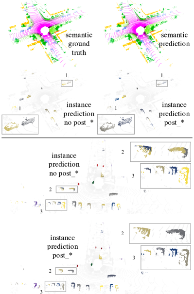
Figure 5: Qualitative results of PanosterK on two challenging samples from the validation set of SemanticKITTI. Enlarged numbered boxes show representative regions.

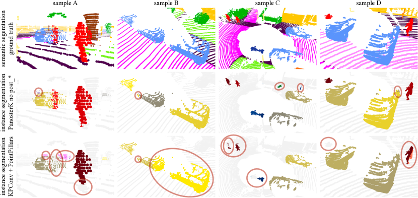
Figure 6: Qualitative comparison on four challenging portions of the validation set of SemanticKITTI, with instance segmentation predicted by our PanosterK without post-processing, and KPConv + PointPillars. In the second and third rows, each color shade represents an ID, while red circles indicate errors.

Semantic improvements. Since Panoster is a bottom-up method, to avoid errors propagating through the things mask, precise semantic segmentation is key for high quality panoptic outputs. Towards this end, we applied the Lovàsz-softmax loss and we limited false negatives by increasing the weight of small instances (denoted by ”small inst. 3x” in Table IV). The former had a positive impact on mIoU, PQ and RQ^Th. The latter, despite decreasing mIoU, increased precision on smaller thing classes, such as person.

Number of predictable clusters N. For all experiments we set N equal to 60, higher than the amount of objects found across the dataset in a single scan. This number can be seen equivalent to the amount of bounding boxes processed in an object detector [25]. Two architectures using N = {60, 90} resulted in a PQ difference of 0.1, showing Panoster insensitivity against N.

Post-processing. As it can be seen in Tables I, II, III and IV, our optional post_* strategies (Section III-D) bring significant improvements to Panoster predictions. They complement our model, fixing its clustering errors through plausibility checks by exploiting 3D data and the task duality of PS. The largest improvement is brought by post_merger, which joins close instances likely to be part of the same object, divided by the model or by post_splitter.

IV-D Runtime Comparison

Our PanosterK model runs on 80K points at 58 FPS at inference time for a single forward-pass on a NVIDIA GTX 1080 8GB GPU, which is 3 FPS (i.e. 5%) slower than its semantic counterpart. Therefore, Panoster brings panoptic capabilities with a relatively small overhead with respect to semantic segmentation networks. This high speed is possible thanks to the simplifications we adopted at inference time (Section IV-A). In comparison, LPSAD, the previously fastest existing method for PS on LiDAR point clouds, runs at 11.8 FPS [10]. Panoster’s built-in learning-based clustering avoids cumbersome grouping strategies to form instances, allowing it to be fast. Moreover, Panoster is more efficient than the combined methods, which require three networks, i.e., one for semantic segmentation, and two for detecting smaller and larger objects [11].

IV-E Qualitative Results

In Fig. 5 we showcase PanosterK predictions on two complex validation scenes, with road intersections and several objects. Each shows the whole 50m radius scan. Despite point sparsity, predictions do not degenerate by increasing the distance from the sensor. Additionally, Panoster is able to distinguish neighboring objects, assigning them different IDs (i.e. colors), as in detail 3 of Fig. 5. Although in challenging scenes, such as the bottom one in the figure, it reuses the same ID for multiple instances, these can be fixed via post-processing as matching IDs are found only in distant objects. We attribute this behavior to the relatively low amount of instances and complex scenes in most training samples.

Furthermore, in Fig. 6 we compare PanosterK, without any post-processing, against the approach proposed in [11] combining KPConv and PointPillars. Qualitative results confirm the findings of our experiments, with our PanosterK delivering superior instance segmentation, with minor errors. Despite relying on a strong object detector, the combined approach completely ignored the challenging pedestrian in sample A next to the car and the partially occluded one in D, wrongly divided a person in D, partially ignored the left person and the rare motorcycle in C, assigned the same ID to multiple people in C, and wrongly detected parked cars in B. As both methods are based on the same semantic architecture, i.e. KPConv, we attribute this difference to the benefit of the integrated panoptic solution offered by our Panoster, as well as to the issues rising from dealing with multiple and possibly contrasting predictions when combining the outputs of various networks.

V Conclusion

In this paper we proposed Panoster: a fast, flexible, and proposal-free panoptic segmentation method, which we evaluated on the challenging LiDAR-based SemanticKITTI dataset, across two different input representations. Panoster outperformed published state-of-the-art approaches, while being simpler and faster. Our method directly delivers instance IDs with a learning-based clustering solution, embedded in the model and optimized for pure and non-fragmented clusters. With its small overhead, Panoster constitutes a valid end efficient approach to extend existing and upcoming semantic methods to perform panoptic segmentation.

References

- [1] Alexander Kirillov, Kaiming He, Ross Girshick, Carsten Rother, and Piotr Dollár, “Panoptic segmentation,” in CVPR, 2019.
- [2] Jonathan Long, Evan Shelhamer, and Trevor Darrell, “Fully convolutional networks for semantic segmentation,” in CVPR, 2015.
- [3] Shaoqing Ren, Kaiming He, Ross Girshick, and Jian Sun, “Faster R-CNN: Towards real-time object detection with region proposal networks,” in NeurIPS, 2015.
- [4] Rohit Mohan and Abhinav Valada, “EfficientPS: Efficient panoptic segmentation,” in arXiv, 2020.
- [5] Lorenzo Porzi, Samuel Rota Bulo, Aleksander Colovic, and Peter Kontschieder, “Seamless scene segmentation,” in CVPR, 2019.
- [6] Bowen Cheng, Maxwell D Collins, Yukun Zhu, Ting Liu, Thomas S Huang, Hartwig Adam, and Liang-Chieh Chen, “Panoptic-DeepLab: A simple, strong, and fast baseline for bottom-up panoptic segmentation,” in CVPR, 2020.
- [7] Xinlong Wang, Shu Liu, Xiaoyong Shen, Chunhua Shen, and Jiaya Jia, “Associatively segmenting instances and semantics in point clouds,” in CVPR, 2019.
- [8] Quang-Hieu Pham, Thanh Nguyen, Binh-Son Hua, Gemma Roig, and Sai-Kit Yeung, “JSIS3D: joint semantic-instance segmentation of 3D point clouds with multi-task pointwise networks and multi-value conditional random fields,” in CVPR, 2019.
- [9] Juana Valeria Hurtado, Rohit Mohan, and Abhinav Valada, “MOPT: Multi-object panoptic tracking,” in CVPR Workshop, 2020.
- [10] Andres Milioto, Jens Behley, Chris McCool, and Cyrill Stachniss, “LiDAR panoptic segmentation for autonomous driving,” in IROS, 2020.
- [11] Jens Behley, Andres Milioto, and Cyrill Stachniss, “A benchmark for LiDAR-based panoptic segmentation based on KITTI,” in arXiv, 2020.
- [12] Stefano Gasperini, Magdalini Paschali, Carsten Hopke, David Wittmann, and Nassir Navab, “Signal clustering with class-independent segmentation,” in ICASSP, 2020.
- [13] Daniel Maturana and Sebastian Scherer, “VoxNet: A 3D convolutional neural network for real-time object recognition,” in IROS, 2015.
- [14] Gernot Riegler, Ali Osman Ulusoy, and Andreas Geiger, “OctNet: Learning deep 3D representations at high resolutions,” in CVPR, 2017.
- [15] Andres Milioto, Ignacio Vizzo, Jens Behley, and Cyrill Stachniss, “RangeNet++: Fast and accurate LiDAR semantic segmentation,” in IROS, 2019.
- [16] Tiago Cortinhal, George Tzelepis, and Eren Erdal Aksoy, “SalsaNext: Fast semantic segmentation of LiDAR point clouds for autonomous driving,” in arXiv, 2020.
- [17] Charles R Qi, Hao Su, Kaichun Mo, and Leonidas J Guibas, “PointNet: Deep learning on point sets for 3D classification and segmentation,” in CVPR, 2017.
- [18] Charles Ruizhongtai Qi, Li Yi, Hao Su, and Leonidas J Guibas, “PointNet++: Deep hierarchical feature learning on point sets in a metric space,” in NeurIPS, 2017.
- [19] Qingyong Hu, Bo Yang, Linhai Xie, Stefano Rosa, Yulan Guo, Zhihua Wang, Niki Trigoni, and Andrew Markham, “RandLA-Net: Efficient semantic segmentation of large-scale point clouds,” in CVPR, 2020.
- [20] Alex H Lang, Sourabh Vora, Holger Caesar, Lubing Zhou, Jiong Yang, and Oscar Beijbom, “PointPillars: Fast encoders for object detection from point clouds,” in CVPR, 2019.
- [21] Hugues Thomas, Charles R Qi, Jean-Emmanuel Deschaud, Beatriz Marcotegui, François Goulette, and Leonidas J Guibas, “KPConv: Flexible and deformable convolution for point clouds,” in ICCV, 2019.
- [22] Yifan Xu, Tianqi Fan, Mingye Xu, Long Zeng, and Yu Qiao, “SpiderCNN: Deep learning on point sets with parameterized convolutional filters,” in ECCV, 2018.
- [23] Deyvid Kochanov, Fatemeh Karimi Nejadasl, and Olaf Booij, “KPRNet: Improving projection-based LiDAR semantic segmentation,” in ECCV Workshop, 2020.
- [24] Haotian Tang, Zhijian Liu, Shengyu Zhao, Yujun Lin, Ji Lin, Hanrui Wang, and Song Han, “Searching efficient 3D architectures with sparse point-voxel convolution,” in ECCV, 2020.
- [25] Kaiming He, Georgia Gkioxari, Piotr Dollár, and Ross Girshick, “Mask R-CNN,” in ICCV, 2017.
- [26] Yuwen Xiong, Renjie Liao, Hengshuang Zhao, Rui Hu, Min Bai, Ersin Yumer, and Raquel Urtasun, “UPSNet: A unified panoptic segmentation network,” in CVPR, 2019.
- [27] Bert De Brabandere, Davy Neven, and Luc Van Gool, “Semantic instance segmentation with a discriminative loss function,” in arXiv, 2017.
- [28] Davy Neven, Bert De Brabandere, Marc Proesmans, and Luc Van Gool, “Instance segmentation by jointly optimizing spatial embeddings and clustering bandwidth,” in CVPR, 2019.
- [29] Martin Ester, Hans-Peter Kriegel, Jörg Sander, Xiaowei Xu, et al., “A density-based algorithm for discovering clusters in large spatial databases with noise.,” in KDD, 1996.
- [30] Ji Hou, Angela Dai, and Matthias Nießner, “3D-SIS: 3D semantic instance segmentation of RGB-D scans,” in CVPR, 2019.
- [31] Li Yi, Wang Zhao, He Wang, Minhyuk Sung, and Leonidas J Guibas, “GSPN: Generative shape proposal network for 3D instance segmentation in point cloud,” in CVPR, 2019.
- [32] Feihu Zhang, Chenye Guan, Jin Fang, Song Bai, Ruigang Yang, Philip HS Torr, and Victor Prisacariu, “Instance segmentation of LiDAR point clouds,” in ICRA, 2020.
- [33] Konstantin Sofiiuk, Olga Barinova, and Anton Konushin, “AdaptIS: Adaptive instance selection network,” in ICCV, 2019.
- [34] Tien-Ju Yang, Maxwell D Collins, Yukun Zhu, Jyh-Jing Hwang, Ting Liu, Xiao Zhang, Vivienne Sze, George Papandreou, and Liang-Chieh Chen, “DeeperLab: Single-shot image parser,” in arXiv, 2019.
- [35] Naiyu Gao, Yanhu Shan, Yupei Wang, Xin Zhao, Yinan Yu, Ming Yang, and Kaiqi Huang, “SSAP: Single-shot instance segmentation with affinity pyramid,” in ICCV, 2019.
- [36] Maxim Berman, Amal Rannen Triki, and Matthew B Blaschko, “The Lovász-Softmax loss: A tractable surrogate for the optimization of the intersection-over-union measure in neural networks,” in CVPR, 2018.
- [37] Jens Behley, Martin Garbade, Andres Milioto, Jan Quenzel, Sven Behnke, Cyrill Stachniss, and Jurgen Gall, “SemanticKITTI: A dataset for semantic scene understanding of LiDAR sequences,” in ICCV, 2019.
- [38] Andreas Geiger, Philip Lenz, and Raquel Urtasun, “Are we ready for autonomous driving? the KITTI vision benchmark suite,” in CVPR, 2012.