Propagation effects in the FRB 20121102A spectra

Abstract

We advance theoretical methods for studying propagation effects in the Fast Radio Burst (FRB) spectra. We derive their autocorrelation function in the model with diffractive lensing and strong Kolmogorov–type scintillations and analytically obtain the spectra lensed on different plasma density profiles. With these tools, we reanalyze the highest frequency 4–8 GHz data of Gajjar et al. (2018) for the repeating FRB 20121102A (FRB 121102). In the data we discover, first, a remarkable spectral structure of almost equidistant peaks separated by ${95\pm 16}$ MHz. We suggest that it can originate from diffractive lensing of the FRB signals on a compact gravitating object of mass $10^{-4}\,M_{\odot}$ or on a plasma underdensity near the source. Second, the spectra include erratic interstellar, presumably Milky Way scintillations. We extract their decorrelation bandwidth ${3.3\pm 0.6}$ MHz at reference frequency 6 GHz. The third feature is a GHz–scale pattern which, as we find, linearly drifts with time and presumably represents a wide–band propagation effect, e.g. GHz–scale scintillations. Fourth, many spectra are dominated by a narrow peak at 7.1 GHz. We suggest that it can be caused by a propagation through a plasma lens, e.g., in the host galaxy. Fifth, separating the propagation effects, we give strong arguments that the intrinsic progenitor spectrum has narrow GHz bandwidth and variable central frequency. This confirms expectations from the previous observations. We discuss alternative interpretations of the above spectral features.

INR-TH-2020-040 arXiv:2010.15145

1 Introduction

Fast Radio Bursts (FRB) still mystify researchers due to unknown nature of their progenitors and anticipation for new propagation effects that may enrich their signals with information on the traversed medium, see reviews by Popov et al. (2018), Petroff et al. (2019), and Cordes & Chatterjee (2019). Sky distribution of the registered bursts is isotropic (Thornton et al., 2013; Shannon et al., 2018) implying that they travel cosmological (Gpc) distances, and localization of several FRB sources confirms that, see Chatterjee et al. (2017); Marcote et al. (2017); Tendulkar et al. (2017); Bannister et al. (2019); Ravi et al. (2019); Prochaska et al. (2019); Marcote et al. (2020); Bhandari et al. (2020). As a consequence, the FRB propagation effects include multi–scale scintillations (Rickett, 1990; Narayan, 1992; Lorimer & Kramer, 2004; Woan, 2011) i.e. diffractive scattering of radio waves on the turbulent plasma clouds in the FRB host galaxy, Milky Way, and in the intervening galactic halos. In addition, the FRB waves may be lensed by refractive plasma clouds with smooth profiles (Clegg et al., 1998; Cordes et al., 2017), or lensed gravitationally by exotic massive compact objects like primordial black holes or dense mini-halos (Zheng et al., 2014; Muñoz et al., 2016; Eichler, 2017; Katz et al., 2020). Thus, studying the FRB signals one may hope to learn something about the cosmological parameters (Deng & Zhang, 2014; Yu & Wang, 2017; Walters et al., 2018; Macquart et al., 2020), intergalactic medium (Zhou et al., 2014; Zheng et al., 2014; Akahori et al., 2016; Fujita et al., 2017), exotic inhabitants of the intergalactic space (Zheng et al., 2014; Muñoz et al., 2016; Eichler, 2017; Katz et al., 2020), and plasma in the far-away galaxies.

The scales of the FRB events point at extreme conditions in their progenitors (Platts et al., 2019) which are hard to achieve in realistic astrophysical settings, see Ghisellini & Locatelli (2018), Lu & Kumar (2018), Katz (2018) and cf. Yang & Zhang (2018), Wang et al. (2019). Millisecond durations of the bursts (Cho et al., 2020) constrain the progenitor sizes to be 100 km or less in the absence of special relativistic effects. Besides, FRB microsecond substructure observed by Nimmo et al. (2021a) limits the instantaneous emission regions down to 1 km. High spectral fluxes (${\sim\mbox{Jy}}$) at GHz frequencies give record brightness temperatures $T\sim 10^{35}-10^{41}\,\mbox{K}$ (Cordes & Chatterjee, 2019; Nimmo et al., 2021b) and therefore support non–thermal, presumably coherent emission mechanisms. The fluxes imply strong (Yang & Zhang, 2020) electromagnetic fields $10^{13}\,\mbox{V}/\mbox{m}$ near the sources which nevertheless should not halt the emission (Ghisellini & Locatelli, 2018). In addition, the periodic activity of the two repeating FRB sources (Amiri et al., 2020; Cruces et al., 2020) points at rotational motions of compact objects and further restricts the progenitor models. Recently an unusually intense radio burst was observed from a Galactic magnetar SGR 1935+2154 (Andersen et al., 2020; Bochenek et al., 2020; Kirsten et al., 2021a) thus marking these objects as main candidates for the FRB sources. Urge to explain the FRB properties and absence of generally accepted theoretical models requires new data. And this field progresses rapidly, see e.g. Tendulkar et al. (2021), Pleunis et al. (2021), Kirsten et al. (2021b), and Rafiei-Ravandi et al. (2021).

Critical information on the FRB central engines can be delivered by their spectra, although a careful data analysis is needed to separate the propagation effects. So far, spectral properties of FRB received undeservingly little attention in the literature, where promising results started to appear only recently, see Gajjar et al. (2018), Hessels et al. (2019), Chawla et al. (2020), Majid et al. (2020), Pearlman et al. (2020), and Pleunis et al. (2021).

With this paper, we develop methods for studying FRB spectral structures and spectral propagation effects, see also Katz et al. (2020). We apply these tools to investigate the frequency spectra of the repeating FRB 20121102A commonly known as FRB 121102 (Spitler et al., 2016; Chatterjee et al., 2017). The bursts were registered at $4-8$ GHz by the Breakthrough Listen Digital Backend at the Green Bank Telescope by Gajjar et al. (2018).

The paper is organized as follows. We introduce the FRB spectra in Sec. 2 and consider their dominating 7.1 GHz peak in Sec. 3. Wide–band pattern and the progenitor spectrum are considered in Sec. 4. In Sec. 5 we study narrow–band scintillations. New periodic spectral structure is analyzed in Sec. 6. In Sec. 7 we compare our narrow–band spectral analysis with the other results. We summarize in Sec. 8. Appendices describe theoretical models used to fit the experimental data.

2 Spectra of FRB 20121102A

Public data of the Breakthrough Listen science team (2018) give de–dispersed spectral flux density $f(t,\,\nu)$ of FRB 20121102A as a function of time $t$ and frequency $\nu$. The provided time intervals include 18 bursts within the first 60 minutes of the 6–hour observations on August 26, 2017. The bursts are assigned identifiers 11A through 11R and 12A through 12C, in order of their arrival. In the wide–band analysis, we suppress the instrumental noise using Gaussian average over the moving frequency window $\sigma=10\,\mbox{MHz}$,

$$\bar{f}_{\sigma}(t,\,\nu)=\int d\nu^{\prime}\,f(t,\,\nu+\nu^{\prime})\;\frac{\mathrm{e}^{-\nu^{\prime 2}/2\sigma^{2}}}{\sigma\sqrt{2\pi}}\;.$$ (1)

By construction, $\bar{f}_{10}$ fairly represents $f$ on scales exceeding $\Delta\nu\geq\pi\sigma\sqrt{2}\approx 45\,\mbox{MHz}$. The modulations at smaller scales $\Delta\nu$ are suppressed by a factor $\exp(-2\pi^{2}\sigma^{2}/\Delta\nu^{2})$. We stress that this smoothing is not used in the analysis of narrow–band scintillations. Note that unlike the simplest binning, Eq. (1) does not rely on a preselected grid of frequencies and therefore does not create bias in the discussion of the spectral periodicity. The color–coded smooth flux densities $\bar{f}_{10}(t,\,\nu)$ of the bursts 11A and 11Q are shown in Fig. 1.

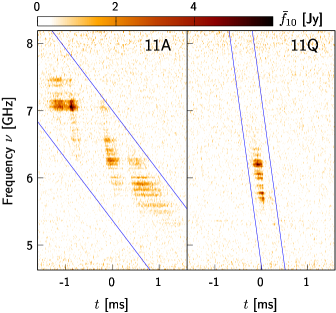
Figure 1: Spectral flux densities $\bar{f}_{10}(t,\,\nu)$ of the bursts 11A and 11Q.

To further visualize the FRB spectra, we integrate $f$ over the burst duration $t_{1}<t<t_{2}$ and obtain its spectral fluence $F(\nu)$ i.e. the burst total energy per unit frequency,

$$\bar{F}_{\sigma}(\nu)=\int\limits_{t_{1}(\nu)}^{t_{2}(\nu)}dt\,\bar{f}_{\sigma}(t,\,\nu)\;,$$ (2)

where the bar again denotes the smoothing Eq. (1). The signal region ${t_{1}(\nu)<t<t_{2}(\nu)}$ (tilted lines in Fig. 1) is chosen in Appendix A to minimize the background noise. The size of this region is about a millisecond, varying from burst to burst. Outside of the signal region $\bar{f}_{10}$ fluctuates around zero. The spectral fluences $\bar{F}_{10}$ of the bursts 11A, 11D, and 11Q are demonstrated in Fig. 2, where the shaded areas near the graphs represent instrumental errors. Apparently, the latter are small and we will ignore them in what follows.

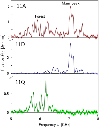
Figure 2: Smoothed spectra of the bursts 11A, 11D, and 11Q. Instrumental errors are displayed with shaded areas near the graphs. Note different scales on the vertical axes.

The spectra in Fig. 2 expose a number of unusual features. First, the graphs 11A and 11D include high and narrow “main peak” at $\nu\approx 7.1\;\mbox{GHz}$. In fact, 10 out of the 18 spectra have this feature precisely at the same position. In some events, e.g. 11D or 11F, this peak carries most of the burst energy. On the other hand, the remaining 8 bursts have no 7.1 GHz peak at all, see the graph 11Q in Fig. 2. Second, almost all spectra display “forests” of smaller peaks of width $\lesssim 100$ MHz. The forests have physical origin, since their presence is not sensitive to the smoothing window $\sigma$ in Eq. (1). Third, the envelopes of the forests have distinctive near–parabolic forms with cutoffs at low and high frequencies. Below we study and explain these three properties.

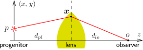
Figure 3: Plasma lens bending the radio ray $p\bm{x}o$.

3 Main peak from the plasma lens

The dominating feature of the most spectra is a high and narrow “main” peak at 7.1 GHz, see the top two panels in Fig. 2. The same peak was observed previously by Gajjar et al. (2018), but it was never explained. Let us argue that it may result from a propagation of the FRB signal through a plasma lens (Clegg et al., 1998; Cordes et al., 2017). Indeed, the latter usually splits the radio wave into multiple rays. Even if the interference of the rays is not relevant, their coalescence at certain frequencies — the lens caustics — may produce high spectral spikes of a specific form.

We consider the lens of Clegg et al. (1998) and Cordes et al. (2017) with dispersion measure depending on one transverse coordinate $x$: ${\mathrm{DM}(x)=\mathrm{DM}_{l}\,\mathrm{e}^{-x^{2}/a^{2}}}$, see Fig. 3. It has two parameters: the size $a$ and central dispersion $\mathrm{DM}_{l}$. Such one–dimensional lenses are often used for modeling plasma overdensities, cf. Cordes et al. (2017). Note that occulting AU–sized structures are expected to be present in turbulent galactic plasmas, and one of them may get on the way of FRB 20121102A. In fact, lensing on such structures is consistent with extreme scattering events observed in the light curves of some active galactic nuclei (Fiedler et al., 1987; Bannister et al., 2016) and perturbations in pulsar timings (Coles et al., 2015). Alternatively, the lens may represent long ionized filament in the supernova remnant from the host galaxy, cf. Graham Smith et al. (2011) and Michilli et al. (2018). Generically, the lens is located in the FRB host galaxy or in the Milky Way, at distances $d_{pl}$ from the source and $d_{lo}$ from us; $d_{po}=d_{pl}+d_{lo}$.

The radio wave receives a dispersive time delay in the lens and as a consequence, propagates along the bended path $p\bm{x}o$ in Fig. 3. These two effects give the phase shift, see Clegg et al. (1998), Cordes et al. (2017), and Appendix B for details,

$$\Phi_{l}(\bm{x})=\frac{1}{2r_{F,\,l}^{2}}\left[-\alpha_{l}a^{2}\,\mathrm{e}^{-x^{2}/a^{2}}+(\bm{x}-\tilde{\bm{x}})^{2}\right]\;,$$ (3)

where the second term comes from the ray geometry, ${\bm{x}=(x,\,y)}$ is the transverse coordinate in the lens plane and its value

$$\tilde{\bm{x}}=(\bm{x}_{p}d_{lo}+\bm{x}_{o}d_{pl})/d_{po}\;.$$ (4)

corresponds to a straight propagation between the transverse positions $\bm{x}_{p}$ and $\bm{x}_{o}$ of the progenitor and the observer. Note that $\tilde{\bm{x}}$ coincides with $\bm{x}_{p}$ when the lens resides in the FRB host galaxy, and $\tilde{\bm{x}}\approx{\bm{x}}_{o}$ if it is close to us. We also introduced the lens Fresnel scale $r_{F,\,l}=(d_{pl}d_{lo}/2\pi\nu d_{po})^{1/2}$ and a dimensionless parameter

$$\alpha_{l}=\frac{2e^{2}r_{F,\,l}^{2}}{a^{2}m_{e}\nu}\;\mathrm{DM}_{l}$$ (5)

characterizing the lens dispersion. Note that $\alpha_{l}^{-1/2}\propto\nu$ is a dimensionless analog of frequency.

In  Clegg et al. (1998) and Cordes et al. (2017) the lens Eq. (3) was solved in the limit of geometric optics $a\gg r_{F,\,l}$. We shortly describe this solution below and give a detailed review in Appendix B. In the geometric limit the radio waves go along the definite paths $\bm{x}_{j}=(x_{j},\,y_{j})$ extremizing the phase Eq. (3). Since the one–dimensional lens bends the rays only in the $x$ direction, $y_{j}=\tilde{y}$ corresponds to a straight propagation, and $x_{j}$ satisfies the nonlinear equation $\partial_{x}\Phi_{l}=0$. One may solve the latter graphically, by plotting $\Phi_{l}(x)$ and identifying the extrema.

Within this approach one can explicitly see that as long as the shift $\tilde{x}$ is small, there exists only one extremal radio path ${x=x_{1}}$ at any $\alpha_{l}$. But above the critical shift $\tilde{x}>{\tilde{x}_{cr}=a(3/2)^{3/2}}$ another two solutions $x_{2},\,x_{3}$ appear at ${\alpha_{-}(\tilde{x})<\alpha_{l}<\alpha_{+}(\tilde{x})}$ i.e. inside a certain frequency interval. Thus, the radio waves with these frequencies propagate along three different paths. The two additional paths coincide, ${x_{2}=x_{3}}$, at the interval boundaries $\alpha_{\pm}$. Besides, the three–path frequency interval is vanishingly small ($\alpha_{+}=\alpha_{-}$) at $\tilde{x}=\tilde{x}_{cr}$ but becomes larger in size at larger shifts $\tilde{x}$.

From the observational viewpoint, the lens focuses or disperses the FRB signal along each path multiplying the intrinsic progenitor fluence $F_{p}$ with the gain factor: ${F=G(\nu)F_{p}}$. In the refractive one–dimensional case the theoretical gain factor

$$G(\nu)=r_{F,\,l}^{-2}\sum_{j}|\partial_{x}^{2}\Phi_{l}(x_{j})|^{-1}$$ (6)

involves second derivatives of the phase at $x=x_{j}$, where we ignore the interference. Thus, the function $G(\nu)$ is infinite at the lens caustics $\partial_{x}^{2}\Phi_{l}=\partial_{x}\Phi_{l}=0$ where two radio paths — the extrema $x_{j}$ of the phase — coalesce. This regime takes place at $\tilde{x}>\tilde{x}_{cr}$ when $G$ becomes infinite at the “frequencies” $\alpha_{\pm}^{-1/2}$ due to coalescence of the paths $x_{2}$ and $x_{3}$. The respective graph of $G$ has a particular two–spike form shown in the inset of Fig. 4b. In reality, the singularities of $G(\nu)$ are regulated by the instrumental resolution / smoothing in Eq. (1) (dashed line in the figure) and wave effects. The regime $\tilde{x}<\tilde{x}_{cr}$ is entirely different, however. In this case the function $G(\nu)$ is smooth, see the inset in Fig. 4a.

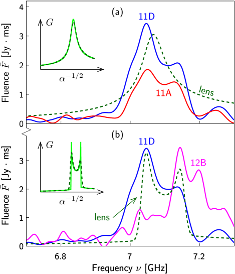
Figure 4: Main peaks of the bursts 11A, 11D, and 12B (solid lines). The graphs 11D are fitted with the smoothed theoretical spectra $\bar{G}_{10}(\nu)F_{p}$ of the lens (dashed) at (a) ${\tilde{x}<\tilde{x}_{cr}}$ and (b) $\tilde{x}>\tilde{x}_{cr}$, where $F_{p}$ is a constant. The insets show $G$ (solid) and $\bar{G}_{10}$ (dashed) as functions of $\alpha_{l}^{-1/2}$ in the respective cases.

The shape of the main peak in the experimental data looks similar to $G(\nu)$. It is particularly tempting to identify the side spikes $\nu_{0}\pm\Delta\nu/2$ of this peak with the positions of the lens caustics in the regime ${\tilde{x}>\tilde{x}_{cr}}$. The maxima of the graph 11D in Fig. 4b give ${\nu_{0}=7.095\;\mbox{GHz}}$ and ${\Delta\nu/\nu_{0}=0.0137}$. In Appendix B.3 we derive analytic expressions for the caustic positions at ${\Delta\nu\ll\nu_{0}}$: Eqs. (B18) and (B19). With the above experimental numbers, they give the source (observer) shift ${\tilde{x}/a\approx 1.885}$ and a combination of the lens parameters

$$\beta\equiv\left(\frac{\mbox{DM}_{l}}{\mbox{pc}\cdot\mbox{cm}^{-3}}\right)\left(\frac{a}{\mbox{AU}}\right)^{-2}\left(\frac{\min\{d_{pl},\,d_{lo}\}}{\mbox{kpc}}\right)$$ (7)

entering $\alpha_{l}$ in Eq. (5): $\beta\approx 0.0355$. Notably, the latter value is consistent with the parameters of the AU–sized structures explaining the extreme scattering events (Fiedler et al., 1987; Bannister et al., 2016; Coles et al., 2015) and parameters of the supernova filaments, cf. Graham Smith et al. (2011).

There is another, qualitatively different fit of the main peak with the lens spectrum. Namely, if $\tilde{x}$ is slightly below critical, the function $G(\nu)$ has a narrow maximum $\nu=\nu_{0}$ with half–height width $\Delta\nu^{\prime}\ll\nu$ near the point where the caustics are about to appear, see the inset in Fig. 4a. One can therefore interpret the major part of the 7.1 GHz peak as the effect of the lens with ${\tilde{x}<\tilde{x}_{cr}}$, ignoring the side spikes. In Sec. 6 we will see that the latter spikes correlate with the short–scale periodic structure of the spectra, so they may be unrelated to a refractive lensing, indeed. We read off $\nu_{0}\approx 7.066\,\mbox{GHz}$ and $\Delta\nu^{\prime}/\nu_{0}\approx 0.014$ from the spectrum 11D in Fig. 4a and use Eqs. (B20), (B21) of Appendix B to compute the lens parameters in this regime: $\beta\approx 0.031$ and $\tilde{x}/a\approx 1.81$.

It is worth recalling that the experimental spectra in Fig. 4 involve smoothing over the frequency intervals ${\sigma=10\,\mbox{MHz}}$. To perform the precise comparison, we smooth the theoretical lens spectra $G(\nu)F_{p}$ in the same way and then fit them to the graph 11D, see the dashed lines in Fig. 4. This procedure almost does not affect the one–peak fit in Fig. 4a but essentially modifies the caustics in the double–peaked lens spectrum in Fig. 4b. We obtain an improved estimate of the lens parameters in the latter case: $\tilde{x}/a\approx 1.890$ and $\beta\approx 0.0359$. In what follows we determine $\tilde{x}/a$ and $\beta$ using the smoothed double–peaked lens spectrum.

So far we completely disregarded the interference of the lensed radio rays which may lead to oscillations of the gain factor with frequency. Note, however, that multiple rays exist only at $\tilde{x}>\tilde{x}_{cr}$ in the narrow frequency interval between the caustics, and we do not see any oscillatory behavior there. To no surprise, since the smoothing Eq. (1) destroys any oscillations on scales below $45\,\mbox{MHz}$. Requiring the interference period to be smaller, we obtain a constraint $a/r_{F,\,l}\gtrsim(\nu/\sigma)^{1/2}\sim 25$ or ${(a/\mbox{AU})^{2}\gtrsim 0.007\cdot\min(d_{pl},\,d_{lo})/\mbox{kpc}}$.

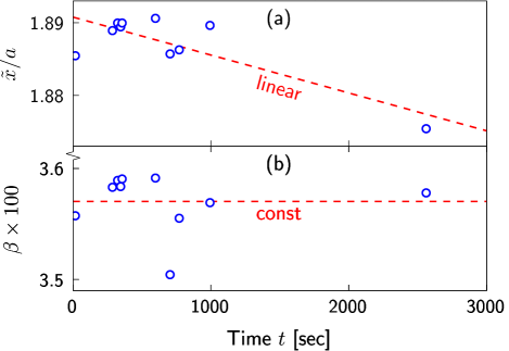
Figure 5: Parameters $\tilde{x}/a$ and $\beta$ of the lens extracted from the main peaks of different burst spectra. Here we use the double–peaked fits at ${\tilde{x}>\tilde{x}_{cr}}$. Note that the main peak is absent in the large interval between the bursts 11M and 12B. We will explain this property in Sec. 4.

To test the lens hypothesis, we compare the main peaks in different FRB spectra. Generically, one expects to find almost time–independent $\beta$ and linearly evolving $\tilde{x}/a$ due to transverse motion of the source/observer with respect to the lens. In Fig. 5 we plot these parameters extracted from the double–peaked fits (Fig. 4b) of different spectra. All values of $\beta$ and $\tilde{x}/a$ are almost identical except for the burst 12B, see the rightmost points in Figs. 5a,b. The “main” peak in the latter burst is slightly different from the others, cf. Fig. 4b. It may or may not represent the same spectral structure. If it does, the shift of its parameter $\tilde{x}$ represents motion of the source relative to the lens. In that case we obtain the relation between the lens relative velocity ${v=d\tilde{x}/dt}$ and its size: ${a\sim 0.3\,\mbox{AU}\cdot v/(200\,\mbox{km}/\mbox{s})}$.

It is worth noting that the narrow bandwidth of the registered FRB spectra and large cosmological $\nu^{-2}$ dispersion precludes analysis of another important lens characteristics: the dispersive time delay of the transmitted FRB signal. The latter depends on frequency in a nontrivial way, distorting the FRB image in the $t$—$\nu$ plane into a peculiar recognizable form, cf. Clegg et al. (1998), Cordes et al. (2017), and Fig. 1.

Overall, the plasma lens hypothesis is very appealing. However, it has visible inconsistencies. First, the spikes in Fig. 4 do not exactly match the main peak slopes and therefore the theoretical fit. Second, the height of this peak relative to the nearby spectrum strongly varies from burst to burst, cf. the bursts 11A and 11D in Fig. 4. Third and finally, some bursts do not have the main peak at all, see the graph 11Q in Fig. 2, as if the lens voluntarily disappears and then appears again with precisely the same parameters.

Two of the above properties will be explained in the forthcoming sections. First, the spectra in Fig. 2 include oscillations, mostly chaotic, at scales below 100 MHz. They certainly deform the main peak. Second, we will observe that the FRB spectra have narrow bandwidth and their central frequency changes from burst to burst. This makes the 7.1 GHz peak vanish if it is outside of the signal band.

4 Wide–band pattern and the progenitor spectrum

It is remarkable that the FRB spectra of Gajjar et al. (2018) are localized in the relatively narrow bands ${\nu_{\mathrm{bw}}\sim\mbox{GHz}}$, but their central frequencies differ significantly. In fact, the same properties were observed before in the measured spectra of FRB 20121102A (Law et al., 2017; Gourdji et al., 2019; Gajjar et al., 2018; Hessels et al., 2019; Majid et al., 2020) and another repeater FRB 20180916B (Chawla et al., 2020; Pearlman et al., 2020). In this Section we are going to show that the wide–band envelopes of our FRB 20121102A spectra are essentially distorted by a spectacular propagation phenomenon similar to wide–band scintillations. Separating this effect, we will give a strong argument that the progenitor spectra themselves are narrow–band and have strongly variable central frequencies.

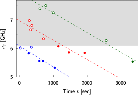
Figure 6: The central frequencies $\nu_{c}$ of the bursts versus their arrival times $t$. Empty and filled points mark the spectra with the pronounced 7.1 GHz peak and without it, respectively. Dashed parallel lines are the linear fits of the data from a given band. The region $\nu_{c}>6.1\;\mbox{GHz}$ is shaded.

To remove the effect of the $7.1\,\mbox{GHz}$ lens, we divide all registered fluences $F(\nu)$ by the lens gain factor $G(\nu)$ determined from the “double–peaked” fit of the spectrum 11D in Fig. 4b. After that we compute the central (“center–of–mass”) frequency of the burst,

$$\nu_{c}\equiv\left(\int_{\nu_{1}}^{\nu_{2}}\nu\,d\nu\,\frac{F(\nu)}{G(\nu)}\right)\Bigg{/}\left(\int_{\nu_{1}}^{\nu_{2}}d\nu\,\frac{F(\nu)}{G(\nu)}\right),$$ (8)

where the integrations are performed over the entire signal region $\nu_{1}<\nu<\nu_{2}$ with positive fluence. It is worth remarking that Eq. (8) uses the original unsmoothed fluence $F(\nu)$.

The central frequency Eq. (8) of the bursts is plotted in Fig. 6 as a function of their arrival time $t$. Notably, the dependence of $\nu_{c}(t)$ is not chaotic! Rather, the central frequencies are attracted to one of the three parallel inclined bands $\nu_{i}(t)$ (dashed lines in Fig. 6) with seemingly random choice of the band.

The bands at $\nu\approx 6$ and 7 GHz have already been noticed by Gajjar et al. (2018) in the summed 4–8 GHz spectrum of FRB 20121102. However, their linear evolution with time has never been observed. Although both observations are made on the basis of limited statistics, they can be tested in the future using larger data samples.

Now, Fig. 6 strongly suggests that the three bands represent a propagation effect, e.g. strong scintillations of the FRB signal in the turbulent interstellar plasma. In this case linear time evolution appears due to relative motion of the observer and progenitor with respect to the scintillating medium. From the physical viewpoint the scintillations are caused by a refraction of the radio waves on the plasma fluctuations which makes them propagate via multiple paths. Interference between the paths then distorts the registered FRB spectra into a pattern of alternating peaks and dips. The bands $\nu_{i}(t)$ in Fig. 6 may represent the scintillation maxima. Then the typical distance between them ${\nu_{d}^{\prime}\sim\nu_{i+1}-\nu_{i}\sim 0.95\;\mbox{GHz}}$ estimates the decorrelation bandwidth.

One traditionally characterizes the scintillating plasma with the diffractive length — the typical transverse distance $r_{\mathrm{diff}}$ at which the correlations between the radio rays die away. This quantity is related to the decorrelation bandwidth as ${\nu_{d}^{\prime}/\nu=(r_{\mathrm{diff}}^{\prime}/r_{F,\,S}^{\prime})^{2}}$, where $r_{F,\,S}^{\prime}$ is the respective Fresnel scale; see Narayan (1992) and Appendix C. We obtain ${r_{\mathrm{diff}}^{\prime}\sim 0.4\,r_{F,\,S}^{\prime}}$. A benchmark property of strong diffractive scintillations is an order–one modulation of the spectra which is observed here, indeed: the regions with strong signal form isolated islands of GHz width, and fluence between them is negligibly small, see Fig. 2.

Importantly, the scintillation pattern is expected to evolve smoothly with time if the source (observer) has a nonzero relative velocity $v$ with respect to the scintillating plasma. This is precisely what we see in Fig. 6: the maxima $\nu_{i}(t)$ drift linearly with the characteristic timescale ${t_{\mathrm{diff}}^{\prime}\simeq 1350\,\mbox{s}}$. Equating ${t_{\mathrm{diff}}^{\prime}\sim r_{\mathrm{diff}}^{\prime}/v}$, we relate the velocity $v$ to ${r_{F,\,S}^{\prime}=(d^{\prime}/2\pi\nu)^{1/2}}$ and hence to the typical distance $d^{\prime}\sim v_{200}^{2}\cdot 2\,\mbox{kpc}$ between the scintillating plasma and the source (observer), where we introduced ${v_{200}=v/(200\,\mbox{km}/\mbox{s})}$.

There remains a question, why the registered spectra have the form of a single relatively narrow signal region despite the fact that the two or three scintillation maxima are usually present in the observation band ${4\,\mbox{GHz}<\nu<8\,\mbox{GHz}}$, cf. Figs. 2, 6. This can happen only if the FRB progenitor has a comparably narrow spectrum with bandwidth $\nu_{\mathrm{bw}}\approx\mbox{GHz}$ which is capable of “illuminating” only one maximum. The same conjecture explains another feature of Fig. 6: all bursts with the main peak (empty circles) have central frequencies within the GHz band around $7.1\,\mbox{GHz}$ (the shaded region in Fig. 6). Note that it would be impossible to explain the disappearance of the main peak in some bursts by destruction of the lens: the shape of this peak remains stable prior to disappearance and recovers later with precisely the same parameters, cf. Figs. 5 and 6.

To sum up, we have argued that the spectrum of the FRB progenitor has $\nu_{\mathrm{bw}}\approx\mbox{GHz}$ bandwidth and its central frequency is changing from burst to burst — chaotically or on short timescale. Note that our argument is based on the separation of the progenitor properties from the wide–band propagation phenomena which strongly distort this spectrum with the unknown frequency shifts of order GHz.

At 1.4 GHz, the registered spectra of FRB 20121102A also occupy a narrow band $\nu_{bw}\sim 200$ MHz or ${\nu_{bw}/\nu\sim}$ 20%, as was observed by Hessels et al. (2019). Note, however, that the entire bandwidth of their instrument is comparable to $\nu_{bw}$. In that case the spectral minima at the band boundaries may be provided by the wide–band scintillations similar to ours. This means that the true bandwidth of the progenitor spectrum may be larger at 1.4 GHz: $\nu_{bw}\gtrsim 200\;\mbox{MHz}$. A different interesting possibility is that the bandwidth of the progenitor spectrum always constitutes 20% of its central frequency. But this latter assumption still has to be tested with the wide–band measurements.

Despite distortions, one can search for the periodic evolution of the progenitor central frequency $\nu_{c}(t)$. We performed this search using the periodogram method described in Zechmeister & Kurster (2009) and Ivanov et al. (2019) at time scales $60-1000\,\mbox{s}$. The best–fit value for a period is 112 s, but the effect is not statistically significant.

5 Narrow–band scintillations

At shorter scales $\Delta\nu\lesssim 100\,\mbox{MHz}$ the spectra in Fig. 2 display seemingly chaotic pattern of alternating peaks and dips. It would be natural to explain this random behavior with another, narrow–band kind of strong interstellar scintillations. Let us show that the latter are indeed present in the FRB 20121102A spectra.

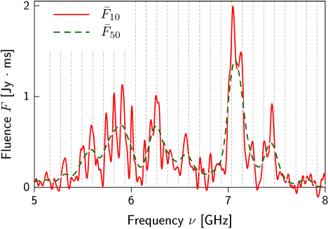
Figure 7: Fluence $F(\nu)$ of the burst 11A smoothed with windows ${\sigma=10\;\mbox{MHz}}$ (solid line) and $50\;\mbox{MHz}$ (dashed). Thin vertical lines display uniform lattice with spacing ${T_{\nu}=\mbox{110.3 MHz}}$.

It is natural to treat the scintillations statistically, i.e. average the spectra over a large ensemble of turbulent plasma clouds and then compare the mean observables to the theory. We recall (Rickett, 1990; Narayan, 1992; Lorimer & Kramer, 2004; Woan, 2011) that different-frequency waves refract differently and therefore go along different paths though statistically independent volumes of the turbulent medium. This makes the scintillating radio spectra uncorrelated at frequencies $\nu$ and $\nu+\Delta\nu$ if $\Delta\nu$ exceeds the decorrelation bandwidth $\nu_{d}$. As a consequence, the statistical average can be performed by integrating over many $\nu_{d}$ intervals. Below we regard the fluence $\bar{F}_{50}(\nu)$ smoothed with large window $\sigma=50\;\mbox{MHz}$ in Eq. (1) as a statistical mean. This quantity indeed delineates a wide–band envelope of the spectrum in Fig. 7 (dashed line) with no trace of the erratic short–scale structure. Note, however, that $\bar{F}_{50}$ should be interpreted with care, since smoothing in Eq. (1) destroys any oscillatory behavior, erratic or not, at frequency periods below $\pi\sigma\sqrt{2}\sim 220\;\mbox{MHz}$.

We introduce the autocorrelation function characterizing the statistical dependence of the spectral fluctuations ${\delta F=F-\bar{F}_{50}}$ at frequencies $\nu$ and $\nu+\Delta\nu$,

$$\mbox{ACF}(\Delta\nu)={\cal N}\int\limits_{\nu_{1}}^{\nu_{2}-\Delta\nu}d\nu\;\;\frac{\delta F(\nu)\delta F(\nu+\Delta\nu)}{\nu_{2}-\nu_{1}-\Delta\nu}\;,$$ (9)

where the data are averaged over the signal bandwidth $\nu_{1}<\nu<\nu_{2}$ by integrating and dividing by the integration interval, whereas the normalization factor ${\cal N}$ makes $\mbox{ACF}(0)=1$. We will see that Eq. (9) is a convenient observable sensitive both to scintillations and periodic structures in the spectra.

Figure 8: (a) The autocorrelation function Eq. (9) of the burst 11A. (b), (c) Its zoom–ins at small $\Delta\nu$. Dashed and solid lines show fits by the theoretical models describing scintillations and scintillations+lensing, Eqs. (10) and (19), respectively.

In Fig. 8 we plot $\mbox{ACF}(\Delta\nu)$ for the burst 11A. It decreases at first indicating that $\delta F(\nu)$ and $\delta F(\nu+\Delta\nu)$ are less correlated at larger $\Delta\nu$. But surprisingly, at $\Delta\nu\gtrsim 50\;\mbox{MHz}$ the autocorrelation function develops a set of wide almost equidistant maxima suggesting that the coherence partially returns! We will consider this effect in the next Section.

Figure 9: Theoretical autocorrelation function $|h(w)|^{2}$ describing Kolmogorov–type scintillations, $w=2\Delta\nu/\nu_{d}$; see Eq. (C29) of Appendix C. It reaches $1/2$ at ${w_{1/2}\approx 1.9}$. Dashed and dotted lines show the approximation Eq. (11) and the Lorentzian fit Eq. (13), respectively.

To interpret the data, we theoretically computed the autocorrelation function for the radio waves strongly refracted in the turbulent plasma with the standard Kolmogorov–type distribution of free electrons, see Appendix C. The result is,

$$\mbox{ACF}={\cal N}\int\limits_{\nu_{1}}^{\nu_{2}-\Delta\nu}\frac{\bar{F}_{50}^{2}(\nu)\;d\nu}{\nu_{2}-\nu_{1}-\Delta\nu}\;\left|h\left(\frac{2\Delta\nu}{\nu_{d}(\nu)}\right)\right|^{2}\;,$$ (10)

where $\bar{F}_{50}\approx\langle F\rangle$ again substitutes the statistical average, while $|h(w)|^{2}$ is a universal hat–like function depicted with the solid line in Fig. 9. Strictly speaking, $h$ is given by the integral (C29), but in practice one can use a very good approximation

$$h(w)\approx[1+a(iw)^{5/6}+(iw/b)^{7/4}]^{-4/7}$$ (11)

capturing the small– and large–$w$ asymptotics of this function and therefore correctly representing it at the intermediate values as well, see the dashed line in Fig. 9. In Eq. (11) we used the numerical coefficients ${a=\frac{7}{8}\Gamma(11/6)}$, $b=\Gamma(11/5)\,2^{6/5}$ and Euler gamma–function $\Gamma(z)$.

The only fitting parameter of the theoretical model Eq. (10) is the value of the decorrelation bandwidth $\nu_{d}(\nu)$ at a given frequency, say, $\nu_{d,\,6}\equiv\nu_{d}(6\;\mbox{GHz})$. At other frequencies the bandwidth is determined from the Kolmogorov scaling

$$\nu_{d}(\nu)=\nu_{d,\,6}\left(\frac{\nu}{6\,\mbox{GHz}}\right)^{4.4}=\nu\;(r_{\mathrm{diff}}/r_{F,\,S})^{2}\;.$$ (12)

The first of these equations is convenient in practice, while the second relates $\nu_{d}$ to the parameters of the scintillating medium: the Fresnel scale $r_{F,\,S}$ characterizing its distancing from the source or the observer and diffractive length $r_{\mathrm{diff}}$ — the transverse separation at which the radio paths decohere inside the medium, see Eqs. (C7) and (C3).

We stress that the theoretical expression (10), (11) is new. Previous studies of Hessels et al. (2019) and Majid et al. (2020) traditionally assumed a Lorentzian ACF profile,

$$h_{L}^{2}={\cal N}\left[c+(\Delta\nu^{2}+\nu_{d,\,L}^{2})^{-1}\right]\;,$$ (13)

which has two parameters: the bandwidth $\nu_{d,\,L}$ and an additive constant $c$. At $c=0$, the fit of our theoretical prediction $|h(w)|^{2}$ with this function gives the dotted line in Fig. 9 and ${\nu_{d,\,L}\approx 1.2\,\nu_{d}}$. Notably, the Lorentzian profile works very well at intermediate frequency lags but, being regular at $\Delta\nu\to 0$, deviates from the theory at small $w$. As a consequence, even at $c=0$ it underestimates the height of the ACF, overestimates its half–height width and gives 20% larger value of $\nu_{d}$. We will see below that the two–parametric Lorentzian fits with arbitrary $c$ are much worse.

Importantly, our theoretical $|h|^{2}$ decreases with $\Delta\nu$ from ${h(0)=1}$ to zero reaching $1/2$ at $\Delta\nu\approx 0.96\,\nu_{d}$. The full autocorrelation functions Eq. (10) have similar profiles and, in particular, monotonically fall off at large $\Delta\nu$. This is the only possible behavior because random fluctuations in the turbulent plasma suppress correlations between the different–frequency waves, and the suppression is stronger at larger $\Delta\nu$. As a consequence, Eq. (10) (dashed line) fits well the initial falloff of the experimental ACF in Fig. 7b giving $\nu_{d,\,6}=3.5\;\mbox{MHz}$. But the same theory fails to explain the peaks at larger $\Delta\nu$ which will be considered in the next Section.

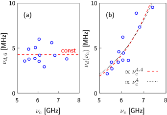
Figure 10: (a) Decorrelation bandwidths $\nu_{d,\,6}=\nu_{d}(6\;\mbox{GHz})$ of the burst spectra versus their central frequencies $\nu_{c}$. (b) Bandwidths $\nu(\nu_{c})$ rescaled to $\nu=\nu_{c}$ via Eq. (12). Dashed lines show fits by Eq. (12): ${\nu_{d}\propto\nu_{c}^{4.4}}$ and $\nu_{d,\,6}=\mbox{const}$. Dotted line in the right panel demonstrates weaker frequency dependence $\nu_{d}\propto\nu_{c}^{4}$.

Overall, we find that the autocorrelation functions of the 12 most powerful bursts match Eq. (10) at small $\Delta\nu$ whereas the weaker bursts 11B, C, G, J, K, M are dominated by the instrumental noise and do not produce discernible correlation patterns at all. From these fits we obtain 12 values of $\nu_{d,\,6}$ in Fig. 10a. The data points group around a constant

$$\nu_{d}(6~{}\mbox{GHz})=4.3\pm 0.9\;\mbox{MHz}$$ (14)

despite the fact that their spectra are localized in essentially different frequency regions. Rescaling the spectral bandwidths $\nu_{d}$ to the burst central frequencies $\nu=\nu_{c}$ via Eq. (12), we obtain the function $\nu_{d}(\nu_{c})$ in Fig. 10b which closely follows the Kolmogorov scaling (dashed line).

The mean value of $\nu_{d}$ fixes the parameter ${r_{\mathrm{diff}}/r_{F,\,S}\approx\mbox{0.027}\pm 0.003}$ of the scintillating plasma. Assuming a galactic distance $d$ to it, we obtain a reasonable diffractive length ${r_{\mathrm{diff}}\sim(1.3\pm 0.1)\times 10^{9}\,\mbox{cm}\times(d/\mbox{kpc})^{1/2}}$, cf. Eq. (C3).

It is worth noting that the frequency integral is an important part of Eq. (10) because the decoherence bandwidth $\nu_{d}$ strongly depends on $\nu$. The theoretical result simplifies, however, in the case $\nu_{2}-\nu_{1}\ll\nu$ when

$$\mbox{ACF}=\left|h(2\Delta\nu/\nu_{d})\right|^{2}$$ (15)

is completely determined by the hat–like function in Eq. (11), while $\nu_{d}$ is computed either at $(\nu_{2}+\nu_{1})/2$ or at $\nu_{c}$ if the spectrum itself is narrow–band. The price to pay, however, is larger statistical fluctuations in the smaller data set. Since our data are relatively narrow–band, we fitted the ACF’s of the 12 strongest bursts by Eq. (15). The respective values of $\nu_{d}(\nu_{c})$ were consistent with Fig. 10b. Using them in Eq. (12), we arrived to ${\nu_{d}(6\;\mbox{GHz})=4.0\pm 0.8\,\mbox{GHz}}$ — almost the same result as before.

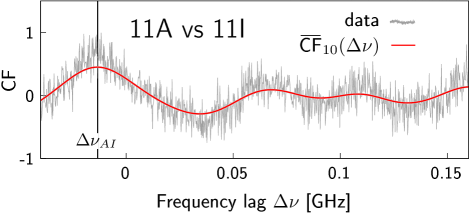
Figure 11: Correlation function $\mbox{CF}(\Delta\nu)$ between the bursts 11A and 11I. To determine its highest maximum (vertical line), we Gauss–smooth this function with window ${\sigma=10\;\mbox{MHz}}$ (smooth solid line).

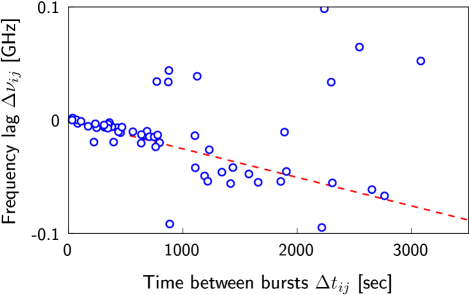
Figure 12: Frequency shifts $\Delta\nu_{ij}$ between the pairs of the burst spectra versus the time $\Delta t_{ij}$ elapsed between them.

We finish this Section with an extra argument, why erratic narrow–band structure stems from a propagation effect, and it is not just a stochastic variation of the progenitor spectrum. First, we compute the correlation functions (CFs) between the pairs of the burst spectra by substituting their fluences ${\delta F_{i}(\nu)\equiv F_{i}-\bar{F}_{50,\,i}}$ and $\delta F_{j}(\nu)$ into Eq. (9) instead of the two identical $\delta F$’s. In particular, in Fig. 11 we plot $\mbox{CF}(\Delta\nu)$ between the bursts 11A and 11I. The highest peak of this function occurs at nonzero $\Delta\nu=\Delta\nu_{AI}$ suggesting that the erratic structures in the spectra are shifted with respect to each other. Moreover, the frequency shift $\Delta\nu_{ij}$ between the different burst pairs linearly depends on the time elapsed between them, see Fig. 12: ${\partial_{t}\Delta\nu_{ij}\approx-2.52\cdot 10^{-2}\;\mbox{MHz}/\mbox{s}}$ (dashed line). Like in the previous Section, we explain this effect by a relative motion of the observer (source) with respect to the scintillating medium (Rickett, 1990; Narayan, 1992; Lorimer & Kramer, 2004; Woan, 2011). The velocity is then roughly estimated as $v\sim r_{\mathrm{diff}}\,\partial_{t}\Delta\nu_{ij}/\nu_{d}\sim 76\,\mbox{km}/\mbox{s}\;(d/\mbox{kpc})^{1/2}$, where the experimental values for $r_{\mathrm{diff}}$ and $\nu_{d}$ are substituted. We obtained a reasonable galactic velocity.

6 Periodic structure

So far we have argued that the peaks of the autocorrelation function in Fig. 8 cannot originate from the scintillations because the latter introduce stronger suppression at larger $\Delta\nu$. The same peaks, however, are naturally explained by the wave diffraction. Indeed, suppose that before or after hitting the scintillating medium the FRB signal passes through the lens — a plasma cloud or a vicinity of a compact gravitating body — which splits it into two radio rays,

$$f=f_{p}\left(G_{1}^{1/2}\,\mathrm{e}^{i\Phi_{1}}+G_{2}^{1/2}\,\mathrm{e}^{i\Phi_{2}}\right)\;,$$ (16)

see one of these rays in Fig. 13. We introduced the intrinsic progenitor signal $f_{p}(\nu)$, gain factors $G_{1,\,2}$ of the rays, and their phases $\Phi_{1,\,2}$. As a consequence of Eq. (16), the net FRB fluence $F=|f|^{2}$ includes an interference term proportional to $\cos(\Phi_{1}-\Phi_{2})$ which oscillates as a function of frequency with the period ${T_{\nu}=2\pi|\partial_{\nu}(\Phi_{2}-\Phi_{1})|^{-1}}$. This enhances correlations between $F(\nu)$ and ${F(\nu+\Delta\nu)}$ at frequency lags equal to the multiples of the frequency period, ${\Delta\nu=nT_{\nu}}$ and therefore produces equidistant peaks in the autocorrelation function Eq. (9).

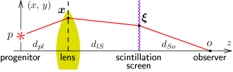
Figure 13: A radio ray passing through the lens and the scintillating medium.

Scintillations obscure the above picture by adding a random component to the wave Eq. (16). In Appendix C we develop an analytic model for the radio waves propagating through the lens and the scintillating plasma. The spectral fluence in this case equals (cf. Eq. (C15)),

$$F=\bar{F}_{50}\left[1+A_{\mathrm{osc}}\;\mathrm{e}^{-\frac{1}{2}(|\tilde{\bm{\xi}}_{1}-\tilde{\bm{\xi}}_{2}|/r_{\mathrm{diff}})^{5/3}}\cos(\Phi_{1}-\Phi_{2})\right]\\ +\delta^{\prime}F\;,$$ (17)

where we extracted a smooth envelope $\bar{F}_{50}(\nu)$ of the spectrum, denoted the relative oscillation amplitude by ${A_{\mathrm{osc}}\equiv 2\sqrt{G_{1}G_{2}}/(G_{1}+G_{2})^{-1}<1}$, and introduced the transverse distance ${|\tilde{\bm{\xi}}_{2}-\tilde{\bm{\xi}}_{1}|}$ between the radio rays inside the scintillating medium. The first line in Eq. (17) represents the statistically averaged contributions of the radio rays and their interference, whereas $\delta^{\prime}F$ denotes fluctuations of the fluence. Scintillations suppress the interference term if the rays go too far apart. We are interested in the unsuppressed regime

$$|\tilde{\bm{\xi}}_{2}-\tilde{\bm{\xi}}_{1}|<r_{\mathrm{diff}}\;.$$ (18)

Notably, in Appendix C we find out that this inequality easily holds for scintillations occurring in our galaxy if the lens is outside of it, cf. Eq. (C30). Or vice versa: one may imagine that the scintillations happen in the FRB host galaxy and the lens is either in the intergalactic space or in the Milky Way.

But even if Eq. (18) holds, the interference peaks of $F(\nu)$ are hidden in the sea of erratic fluctuations $\delta^{\prime}F$. The latter have order–one amplitude if the scintillations are strong: $\delta^{\prime}F\sim F$, cf. Fig. 7. To separate the two effects, one uses the autocorrelation function Eq. (9) where the frequency integral averages the fluctuations away. In Appendix C we derive ACF for the theoretical model with scintillations$+$lensing,

$$\mbox{ACF}={\cal N}\int_{\nu_{1}}^{\nu_{2}-\Delta\nu}d\nu\;\frac{\bar{F}_{50}(\nu)\bar{F}_{50}(\nu+\Delta\nu)}{\nu_{2}-\nu_{1}-\Delta\nu}\;\\ \times\Big{[}\,|h|^{2}+\frac{1}{2}A_{\mathrm{osc}}^{2}\,\left(1+|h|^{2}\right)\,\cos(2\pi\Delta\nu/T_{\nu})\Big{]}\;,$$ (19)

where $h\equiv h(2\Delta\nu/\nu_{d}(\nu))$ is the same “scintillation” function (11) as before, $\nu_{d}(\nu)$ is given by Eq. (12), and the frequency period $T_{\nu}$ is already extracted from $\Phi_{2}-\Phi_{1}$. Note that Eq. (19) is valid at $\nu_{d}\ll\nu$ with the corrections of order $(\nu_{d}/\nu)^{1/3}\sim 8\%$.

The theoretical expression (19) describes both the initial falloff of the autocorrelation function due to scintillations and the periodic peaks at ${\Delta\nu=nT_{\nu}}$ caused by the two–ray interference. It fits well the experimental data in Fig. 8 (solid line) giving $\nu_{d}\approx 2.4\;\mbox{MHz}$, ${T_{\nu}\approx 110.3\;\mbox{MHz}}$, and $A_{\mathrm{osc}}\approx 0.5$ for the burst 11A.

Figure 14: Autocorrelation function of the burst 11D.

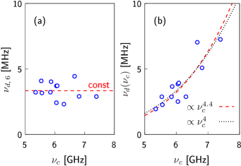
Figure 15: (a) Decorrelation bandwidths ${\nu_{d,\,6}\equiv\nu_{d}(6\;\mbox{GHz})}$ of the burst spectra extracted from the full fits Eq. (19) of their ACFs that take into account the periodic structure. (b) Bandwidths $\nu_{d}(\nu_{c})$ rescaled to the central frequencies of their bursts via Eq. (12). Dashed lines represent the mean bandwidth ${\nu_{d,\,6}\approx 3.3\pm 0.6\,\mbox{MHz}}$ rescaled with Eq. (12). The dotted line shows weaker dependence $\nu_{d}\propto\nu_{c}^{4}$ for comparison.

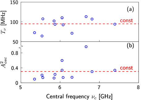
Figure 16: (a) Frequency periods $T_{\nu}$ and (b) amplitude squares $A_{\mathrm{osc}}^{2}$ of the spectral oscillations in bursts with central frequencies $\nu_{c}$.

In fact, the autocorrelation functions of the strongest bursts, e.g. 11A or 11D, display easily recognizable sets of periodic peaks, see Fig. 14, and many other bursts include hints of those. Fitting ACFs of the 12 most powerful spectra with Eq. (19), we obtain the respective decorrelation bandwidths $\nu_{d}$, frequency periods $T_{\nu}$, and amplitudes $A_{\mathrm{osc}}$ in Figs. 15 and 16.

The frequency periods in Fig. 16a group within the $15\%$ interval around the mean value $T_{\nu}\approx 95\pm 16\;\mbox{MHz}$ and do not indicate any dependence on frequency. At the same time, the jumps of $A_{osc}^{2}$ in Fig. 16b are much larger. This sensitivity can be explained by the fact that some weak ACF’s include only hints of the periodic patterns and give very small $A_{osc}$, while the other have barely discernible initial “scintillation” falloffs, hence an overestimate of $A_{osc}$. In what follows we use $A_{osc}\approx 0.5$ obtained by averaging the 12 points in Fig. 16b (dashed line).

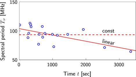
Figure 17: Periods $T_{\nu}$ of spectral oscillations in different bursts versus their arrival times (points). Solid and dashed lines show fits by linear time evolution and a constant, respectively.

In Fig. 17 we plot the frequency periods of different bursts versus their arrival times. The data points are consistent with the time–independent $T_{\nu}$ (dashed line), although a slow evolution with ${dT_{\nu}/dt\approx-1.1\cdot 10^{-2}\,\mbox{MHz}/\mbox{s}}$ is also possible (solid line).

The fit Eq. (19) gives an improved estimate of the burst scintillation bandwidths $\nu_{d,\,6}$ and $\nu_{d}(\nu_{c})$, see Figs. 15a,b and recall Fig. 10. Now, the data group a bit closer, and they still agree with the prediction of the Kolmogorov turbulence Eq. (12) (dashed lines). The averaging gives ${\nu_{d}(6\;\mbox{GHz})\approx(3.3\pm 0.6)\,\mbox{MHz}}$.

Now, we can explicitly visualize the periodic pattern in the burst spectra. In Fig. 7 we plotted the smoothed fluence $\bar{F}_{10}(\nu)$ of the burst 11A together with the lattice of the vertical dotted lines separated by ${T_{\nu}=110.3\;\mbox{MHz}}$ — a frequency period of the respective ACF in Fig. 8. By construction, smoothing with ${\sigma=10\,\mbox{MHz}}$ kills almost all narrow–band scintillations because ${\nu_{d}\ll\pi\sigma\sqrt{2}}$. As a consequence, the highest maxima in Fig. 7 should belong to the periodic structure. Indeed, too many of them are close to the dotted lines. Moreover, the side spikes of the “main” 7.1 GHz peak seem to be a part of the same structure.

We demonstrated that the two–ray interference correctly describes the leading periodic behavior of the spectra. Nevertheless, there are visible inconsistencies. First, the experimental autocorrelation functions in Figs. 8a, 14 deviate from the fits in some places. Second, there are burst–to–burst variations in ACFs leading to 15% spread of $T_{\nu}$ values in Fig. 16a. Third, some maxima in Fig. 7 are off the periodic grid.

All these effects are expected. On the one hand, strong erratic GHz– and MHz–scale scintillations exist in the spectra; without any doubt, the ones with $\nu_{d}\sim 100$ MHz are present as well. They slightly shift the maxima in Fig. 7 and add smaller peaks. Moreover, unlike the strongest narrow–band fluctuations which are averaged via the frequency integral in Eq. (9), the ones with larger $\nu_{d}$ remain almost random. They stochastically distort the expected cos–like behavior of the ACFs in Figs. 8a, 14 and penetrate into the fit results for $T_{\nu}$. On the other hand, we use the simplest two–wave interference model and disregard the subdominant rays altogether. But generically, the latter are present in the data along with their subdominant interference contributions distorting the graphs. One can take these features into account at the cost of adding new parameters to the fits.

In fact, the structure similar to what we see in Fig. 7 was observed in the High–Frequency Interpulses (HFI) of the Crab pulsar, see Hankins et al. (2016). Namely, the spectra of HFI consist of many isolated bands with inter–band distance ${\nu_{\mathrm{band}}\simeq 0.06\,\nu}$. In turn, every band includes $\sim 3$ sub–bands. At 6 GHz this gives ${\nu_{\mathrm{band}}\simeq 344}$ MHz and $\sim 100$ MHz of sub-band distance. Intriguingly, the wide–band envelope $\bar{F}_{50}$ of the FRB spectrum in Fig. 7 has several maxima separated by $\nu_{\mathrm{band}}\simeq 330$ MHz which consist, at a higher spectral resolution, of the equidistant peaks with period $T_{\nu}\approx 110$ MHz. This resemblance may suggest similar mechanisms operating in Crab and in FRB 20121102A. Note that $T_{\nu}\propto\nu$ does not contradict to the points in Fig. 16a which have a spread.

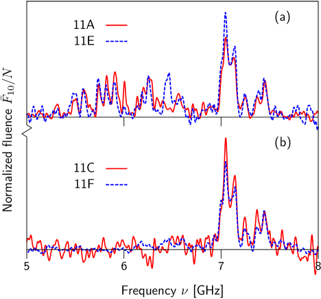
Figure 18: Normalized fluences of the (a) bursts 11A and 11E; (b) bursts 11C and 11F. The area under each graph equals one.

Let us argue that the entire 100  MHz spectral pattern including the periodic structure and subleading peaks originates from the propagation phenomena. We divide the smoothed spectra $\bar{F}_{10}(\nu)$ by their total energy releases making the areas under their graphs equal to one. After that some of the normalized spectra look almost identical to each other, like the twin brothers, cf. the graphs 11A and 11E in Fig. 18a, or 11C and 11F in Fig. 18b. Notably, these coinciding bursts are not sequential, e.g. 11A is followed by the bursts B to D, and only then by the burst E. Such similarity would be very hard to explain by the intrinsic properties of the emission mechanism. In the model with diffractive lensing and scintillations the effect is provided by small velocities of the lenses and the scintillating media and by the randomized central frequency of the FRB progenitor. The FRB signals acquire the same narrow–band spectral structure if they are localized in the same frequency band and occur shortly after one another, so that the lens and the medium do not have enough time to evolve.

Figure 19: (a) The sum of the normalized spectra for the 12 most powerful bursts. The result is smoothed with $\sigma=10\;\mbox{MHz}$ and shown in units of the maximum. The lattice of equidistant vertical lines has spacing ${T_{\nu}=97\;\mbox{GHz}}$. (b) ACF of the summed spectrum and its fit with Eq. (19).

We perform another important test by summing up the normalized spectra of the 12 most powerful bursts. The result is more noisy than the strongest 11D and 11A spectra because the weaker bursts give the same–order contributions into the normalized sum. The summed spectrum is visualized in Fig. 8, where smoothing with $\sigma=10\;\mbox{MHz}$ is used. One finds that many of its maxima appear near the periodic lattice of dashed vertical lines. Besides, the ACF of this summed spectrum (Fig. 19b) includes many almost equidistant peaks at large $\Delta\nu$. Fitting this function with Eq. (19), we obtain the frequency period $T_{\nu}\approx 97\;\mbox{MHz}$ and decorrelation bandwidth ${\nu_{d}\approx 4.45\;\mbox{MHz}}$ which are close to our previous results. Notably, the fit is pretty good: note that the positions of the ACF peaks in Fig. 19b correlate with the periodic maxima of the fitting function over many periods. We conclude that the periodic structure is stable in time and not peculiar to the strongest bursts.

It is worth discussing possible theoretical models for the lens which splits the FRB wave into two rays and creates the periodic spectral structure. First, it may be formed by a plasma residing, say, in the FRB host galaxy. Consider e.g. the one–dimensional Gaussian lens of Sec. 3 with the phase shift,

$$\Phi_{l}=\frac{1}{2r_{F,\,l}^{\prime 2}}\left[(x-\tilde{x}^{\prime})^{2}+\alpha_{l}^{\prime}a^{\prime 2}\,\mathrm{e}^{-x^{2}/a^{\prime 2}}\right]\;.$$ (20)

Here we equipped all the lens parameters with the primes and ignored the trivial dependence on $y$ leaving only one transverse coordinate $x$. We also changed the sign in front of the second term, so now the lens with ${\alpha_{l}^{\prime}\propto-\delta n_{e}>0}$ describes an underdensity of free electrons. For simplicity below we assume $\ln\alpha_{l}^{\prime}\gg 1$ and $\tilde{x}^{\prime}\sim a^{\prime}\sqrt{\ln\alpha_{l}^{\prime}}$ — a strong lens relatively far away from the line of sight.

Note that the underdensities are expected to appear in the interstellar medium due to heating, e.g., by the magnetic reconnections. They were often used to explain the pulsar data. For example, Pen & King (2012) interpreted the pulsar extreme scattering events (ESEs) as lensing on the Gaussian underdensities Eq. (20). Another type of underdensity lenses in the form of corrugated plasma sheets was suggested to cause pulsar scintillation arcs in Simard & Pen (2018). We will demonstrate that the lens Eq. (20) can explain the diffractive peaks in our data.

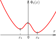
Figure 20: Phase delay Eq. (20) in the Gaussian underdensity lens.

The phase delay Eq. (20) is plotted in Fig. 20. It has three extrema corresponding to three radio rays. In Appendix B.4 we argue that the ray with $x\approx 0$ has small gain factor and can be ignored, while the other two give Eq. (16). Computing the parameters of these rays, we obtain

$$A_{\mathrm{osc}}\approx\sqrt{1-\frac{\tilde{x}^{\prime 2}}{a^{\prime 2}\ln\alpha_{l}^{\prime}}}\;,\qquad T_{\nu}\approx\frac{\pi\nu r_{F,\,l}^{\prime 2}}{a^{\prime}\tilde{x}^{\prime}\sqrt{\ln\alpha_{l}^{\prime}}}\;.$$ (21)

The experimental values $A_{osc}\approx 0.5$ and $T_{\nu}\approx 95\;\mbox{MHz}$ then give ${\tilde{x}\approx a^{\prime}\sqrt{\ln\alpha_{l}^{\prime}}}$ and ${r_{F,\,l}^{\prime}\approx 0.07\,a^{\prime}\sqrt{\ln\alpha_{l}^{\prime}}}$, where realistically, $\ln\alpha_{l}^{\prime}\sim 3-10$.

The second option includes lensing of the FRB signal on the gravitating compact (point–like) object of mass $M$, e.g. a primordial black hole or a dense mini–halo, like in Katz et al. (2020). The total phase delay in this case has the form similar to Eq. (20), see Peterson & Falk (1991), Matsunaga & Yamamoto (2006), Bartelmann (2010):

$$\Phi_{l}=\frac{1}{2r_{F,\,l}^{\prime 2}}\left\{(\bm{x}-\tilde{\bm{x}}^{\prime})^{2}-2(d_{lo}^{\prime}\theta_{E})^{2}\ln\left|\frac{\bm{x}-\bm{x}_{o}}{d_{lo}^{\prime}}\right|\right\}\,,\!\!$$ (22)

where $d_{lo}^{\prime}$ is the distance to the object, $\tilde{\bm{x}}^{\prime}$ is given by Eq. (4) with the parameters of the new lens, $r_{F,\,l}^{\prime}$ is the respective Fresnel scale, and $\theta_{E}=(4GMd_{pl}^{\prime}/d_{lo}^{\prime}d_{po})^{1/2}$ is the Einstein angle. Now, the second term in the phase shift is caused by gravity rather than refraction. That is why it is proportional to the frequency of the radio wave and mass of the lens: $(\theta_{E}/r_{F,\,l}^{\prime})^{2}\propto\nu M$.

Generically, the point–like gravitational lens splits the radio wave into two rays in Eq. (16). Computing the respective eikonal solutions, one finds,

$$A_{\mathrm{osc}}=\frac{2}{\zeta^{2}+2}\;,\qquad$$ (23)

$$T_{\nu}=\frac{1}{4GM}\,\left[\zeta\sqrt{\zeta^{2}+4}+2\ln(\zeta/2+\sqrt{\zeta^{2}/4+1})\right]^{-1}\;,$$

see Appendix B.5 and Peterson & Falk (1991), Matsunaga & Yamamoto (2006), Bartelmann (2010), Katz et al. (2020) for details. Here we introduced the angular separation of the source from the lens in units of the Einstein angle ${\zeta=|\bm{x}_{p}-\bm{x}_{o}|/(\theta_{E}d_{lo}^{\prime})}$. Substituting the mean experimental values of $A_{\mathrm{osc}}$ and $T_{\nu}$, we obtain ${\zeta\approx 1.4}$ and $M\approx 1.1\cdot 10^{-4}\,M_{\odot}$.

Let us guess, where the gravitational lens lives. It is natural to assume that such exotic objects constitute a part $\gamma$ of dark matter. Then the probability of meeting one of them in the intergalactic space at distance $|\bm{x}_{p}-\bm{x}_{o}|\lesssim\zeta\theta_{E}d_{lo}^{\prime}$ from the line of sight is of order ${\gamma\zeta^{2}G\rho_{m}d_{po}^{2}\sim 10^{-2}\,\gamma}$, where we substituted $\zeta\approx 1.4$, the distance to the source $d_{po}\sim\mbox{Gpc}$, and the mean dark matter density ${\rho_{m}\sim 3\cdot 10^{-6}\;\mbox{GeV}/\mbox{cm}^{3}}$. Thus, the gravitational lensing of one FRB signal is relatively unprobable even if all dark matter consists of lenses. However, the probability of the respective event inside the galactic halo of Mpc size is $\sim 10$ times smaller despite the larger density. Thus, the gravitational lensing is generically expected to occur on the way between the galaxies.

It would be great to discriminate between the above two lenses on the basis of the spectral data alone. For example, one may assume that the dependence of the frequency period $T_{\nu}$ on frequency $\nu$ is different in the two cases. Indeed, universality of the gravitational lensing gives $T_{\nu}(\nu)=\mbox{const}$, whereas refraction of radio waves in the plasma is essentially $\nu$–dependent. Note, however, that the first (geometric) term of the plasma lens phase shift Eq. (20) is proportional to the frequency, just like the gravitational shift Eq. (22). If it is important, the dependence of the frequency period on $\nu$ may be extremely weak. An example is provided above by the strong underdensity lens. In this case the values of $A_{\mathrm{osc}}$ and $T_{\nu}$ in Eq. (21) logarithmically depend on $\nu$ via the lens strength $\alpha_{l}^{\prime}\propto\nu^{-2}$ and become indistinguishable from constants at $\alpha_{l}^{\prime}\gtrsim 5$.

Nevertheless, it is worth stressing that the experimental data do not indicate any dependence of the spectral oscillation parameters on frequency. Indeed, the values of $T_{\nu}$ in Fig. 16a are almost the same for the bursts with essentially different central frequencies $\nu_{c}$.

7 Comparison with earlier studies

Our analysis of the narrow–band spectral structure essentially differs from the previous ones. Let us explain the distinction and place our results in the context of the other FRB 20121102A studies.

Figure 21: Autocorrelation functions of the two FRB 20121102A bursts B1 and B6 at frequency 2.24 GHz (Figure 3 of Majid et al. (2020)). Panels (a) and (c) show their initial falloffs at ${\Delta\nu<0.84\;\mbox{MHz}}$, while (b) and (d) cover larger $\Delta\nu$ intervals.

The unusual features were observed in the burst autocorrelation functions before, but a conclusive evidence for their diffractive origin has never appeared. For example, Majid et al. (2020) published two ACFs of the FRB 20121102A bursts B1 and B6 measured by the DSS–43 telescope of the Deep Space Network at frequency 2.24 GHz, see Fig. 21. At large $\Delta\nu$ these functions display several recognizable maxima, see Figs. 21b,d. Interpreting the latter as a manifestation of the two–wave interference, one can formally fit the B1 and B6 ACFs with the cos–like function in the integrand of Eq. (19) plus a constant. The results of this fit are shown by the dash–dotted lines in Figs. 21b,d. The respective best–fit frequency periods are $T_{\nu}\approx 3.5$ and $1.4\;\mbox{MHz}$ for the bursts B1 and B6, respectively.

Note, however, that unlike the BL digital backend of the Green Bank Telescope, the instrument of Majid et al. (2020) has narrow 8 MHz non–contiguous sub-bands. As a consequence, the graphs B1 and B6 in Fig. 21 include only 2 and 4 peaks in the available frequency interval, and one cannot judge whether they are periodic or not. Compare this to the strongest bursts 11A and 11D in Figs. 8a and 14, every one of which displays $\sim 10$ approximately equidistant ACF maxima. Besides, the apparent frequency periods $T_{\nu}$ of the bursts B1 and B6 mismatch by a factor of 2. The data of the previous Section were consistent: the values $T_{\nu}$ of the 12 strongest bursts were grouping within the 15% interval near the central value. Finally, the widths of the maxima in Fig. 21 are comparable to the entire frequency interval $\nu_{2}-\nu_{1}=8\;\mbox{MHz}$. In fact, the presence of the unsuppressed random fluctuations is expected at these scales, since the frequency integral in the ACF effectively kills only the noise with $\nu_{d}\ll\nu_{2}-\nu_{1}$, cf. Eq. (9).

We conclude that the periodic structures cannot be distinguished from the random spectral behavior in Majid et al. (2020) data. To do that, one needs wide–band measurements of many spectra, like the ones performed by the Green Bank Telescope.

Now, let us compare our new method of studying the scintillations with the previous ones. Gajjar et al. (2018) performed the original analysis of the 4–8 GHz Green Bank Telescope data by fitting the sub–band autocorrelation functions with the Gaussian profiles at ${\Delta\nu<200\;\mbox{MHz}}$. The resulting values of $\nu_{d}$ — the half width at half maximum of the fitting function — were found to be consistent with $\nu_{d}\approx 24\;\mbox{MHz}$ at 6 GHz, which is 6–7 times larger than our result. This huge discrepancy is related to the fact that the fitting interval $\Delta\nu<200\;\mbox{MHz}$ in Gajjar et al. (2018) includes the first equidistant ACF maximum, see Fig. 8. This new feature is enveloped by the fitting function making the latter wider. On the other hand, we fitted only the initial part of the ACF to the left of its first minimum.

Majid et al. (2020) obtained the decorrelation bandwidth of the two FRB 20121102A bursts B1 and B6 using the 2.4 GHz DSS–43 telescope data. To this end the initial falloffs of the respective ACFs were fitted with the Lorentzian profile Eq. (13) at $\Delta\nu<0.84\;\mbox{MHz}$, where ${\cal N}$, $\nu_{d}$, and $c$ served as the fit parameters, see Cordes et al. (1985). The result was $\nu_{d}\approx 180\;\mbox{kHz}$ and 280 kHz for the bursts B1 and B6, respectively. We replot the Majid et al. (2020) data and their Lorentzian fits in Fig. 21 (steps and solid lines). Their procedure is different from ours in two important respects. First, we fix $c$ — the constant part of the ACF — with the subtraction procedure which effectively means that $c$ tracks the mean value of this function at large $\Delta\nu$, cf. Eq. (9). Indeed, if one leaves this parameter free in the fit, its value would essentially depend on the $\Delta\nu$ interval and, crudely speaking, would pick up the minimal value of the autocorrelation function at the interval boundary. This sensitivity is an artifact of the unexpected ACF oscillations at large $\Delta\nu$, and it is not correct. One can fix the arbitrariness in our manner by fitting the ACF’s at large $\Delta\nu$ with the constant $c$ (dotted horizontal lines in Fig. 21) and then performing the stable Lorentzian fit at small $\Delta\nu$. The fit result is $\nu_{d}(2.24\;\mbox{GHz})\approx 155\pm 14\;\mbox{kHz}$ and $162\pm 20\;\mbox{kHz}$ for for the bursts B1 and B6, respectively. Notably, the two values of the decorrelation bandwidth now agree within the errorbars obtained from the fits.

Second, we use new theoretical profile Eq. (11), (15) for the ACF which has sharper behavior as ${\Delta\nu\to 0}$, see Fig. 9. As discussed in the previous Section, this method generically gives 20% smaller value of $\nu_{d}$. Indeed, for the bursts B1 and B6 we obtain $\nu_{d}\approx 128\;\mbox{kHz}$ and 133 kHz at a reference frequency 2.24 GHz, see the dashed lines in Figs. 21a,c.

Now, we rescale the decorrelation bandwidth ${\nu_{d}\approx 130\;\mbox{kHz}}$ at 2.24 GHz to our frequencies. Using the Kolmogorov formula (12) with $\nu_{d}\propto\nu^{4.4}$, we obtain $\nu_{d}\approx 9.9\;\mbox{MHz}$ at 6 GHz, which is 2–3 times larger than our values: recall that the “scintillations” and “scintillations+lensing” fits of the previous Sections give ${\nu_{d}(6\;\mbox{GHz})\approx 4.3}$ and 3.3 MHz, respectively. This means that non–Kolmogorov frequency dependence $\nu_{d}\propto\nu^{\alpha}$ with $\alpha<4.4$ is favored by the data. In particular, rescaling with $\alpha=4$ gives $\nu_{d}\approx 6.7$ MHz at 6 GHz which differs from our values by the “reasonable” factor of 2. At even smaller $\alpha=3.5$ one finds $\nu_{d}(6\;\mbox{GHz})\approx 4.1$ MHz in agreement with our result.

Note that non–Kolmogorov scaling $\nu_{d}\propto\nu^{\alpha}$ with ${\alpha<4.4}$ was observed in the Milky Way pulsar signals, see e.g. Bhat et al. (2004). Moreover the pulsar data coming from certain directions suggest $\alpha=3-4$ which is not theoretically possible for weakly coupled turbulent plasma. Our result is of this kind.

Another value $\nu_{d}\approx 58\;\mbox{kHz}$ at 1.65 GHz was obtained by  Hessels et al. (2019) using European VLBI Network data for one FRB 20121102A burst. This result corresponds to $\nu_{d}\approx 17$, 10, and 5.3 MHz at 6 GHz in the cases $\alpha=4.4$, $4$, and $3.5$, respectively. The result at $\alpha=4$ is again twice larger than ours while the one with $\alpha=3.5$ is a good match.

Finally, let us compare the value of $\nu_{d}$ with the prediction of NE2001 model for the Milky Way distribution of free electrons (Cordes & Lazio, 2002). Extracting the scattering measure in the direction of FRB 20121102A from the provided software and using Eq. (10) of Cordes & Lazio (2002), we obtain the scintillation bandwidth in our galaxy: $\nu_{d,\;gal}\approx 21\,\mbox{MHz}$ at 6 GHz. This result again assumes Kolmogorov scaling and it is 5–6 times larger than our experimental values. To feel how the prediction of the model would change in the non–Kolmogorov case, recall that Cordes & Lazio (2002) mostly use the pulsar data with typical frequencies in the GHz range, cf. Majid et al. (2020). Thus, scaling with powers $\alpha=4$ and 3.5 would give $6^{4.4-\alpha}$ times smaller bandwidths ${\nu_{d,\;gal}\approx 10}$ and 4.2 MHz. Once again, we obtain factor two difference and a perfect match at $\alpha=4$ and $3.5$, respectively.

To sum up, the bandwidth $\nu_{d}$ of our narrow–band scintillations differs by factors of several from the two measurements at other frequencies and from the prediction of the NE2001 model if the Kolmogorov scaling is assumed. In the case of non–Kolmogorov frequency dependence $\nu_{d}\propto\nu^{4}$ the four results agree up to a factor of two. If $\nu_{d}\propto\nu^{3.5}$, all results match perfectly. Note that non–Kolmogorov scaling with $\alpha=3.5$ or 4 does not contradict to our data in Figs. 10b and 15b (dotted lines) and in fact is observed in the pulsar measurements (Bhat et al., 2004; Geyer et al., 2017).

8 Conclusions and Discussion

In this paper we reanalyzed the spectra of FRB 20121102A measured by Gajjar et al. (2018). We developed practical theoretical tools to study the random spectral components, regular peaks and periodic spectral structures which may be caused by interstellar scintillations, refractive and diffractive lensing, or, alternatively, can be intrinsic to the FRB progenitor.

We saw that the caustics of the refractive lens produce a spectral peak of a distinctive recognizable form (Clegg et al., 1998; Cordes et al., 2017) that can be directly fitted to the spectra. On the other hand, separation of diffractive lensing from scintillations requires calculation of an integral observable: the spectral autocorrelation function (ACF) in Eq. (9). The scintillations are responsible for the monotonic falloff of this function with frequency lag $\Delta\nu$, while the two–ray diffraction introduces a distinctive oscillatory behavior i.e. the series of pronounced equidistant maxima. We derived explicit theoretical expressions for the ACFs which include the effects of Kolmogorov–type scintillations and scintillations on top of diffractive lensing, Eqs. (10), (11) and (19), respectively. The latter expressions can be used to interpret the experimental data, and in fact, fit them quite nicely. An alternative data analysis may involve Fourier transform as in Katz et al. (2020), periodogram method in Zechmeister & Kurster (2009), Ivanov et al. (2019), or Kolmogorov–Smirnov–Kuiper test in Press et al. (2007).

Using the above tools, we identify and explain several remarkable features in the FRB 20121102A spectra. First and most importantly, we discover a set of almost equidistant spectral peaks separated by ${T_{\nu}=95\pm 16\;\mbox{MHz}}$. This periodicity is a benchmark property of wave diffraction, and we show that it may be relevant, indeed. On the one hand, the peaks may be caused by diffractive gravitational (femto)lensing of the FRB signals on a compact object of mass $10^{-4}\,M_{\odot}$, e.g. a primordial black hole or a dense minihalo, see Katz et al. (2020). Theoretically, such events are expected to occur with relatively small probability $\sim 10^{-2}$ in the intergalactic space if all dark matter consists of lenses. On the other hand, the periodic peaks may originate from the diffractive lensing on a plasma underdensity in the host galaxy. The respective lenses — the holes in the electron density — may be expected to appear due to plasma heating and in fact, are discussed in the literature, see e.g. Pen & King (2012) and Simard & Pen (2018).

Yet another suggestion would be to attribute the periodic structure to the progenitor spectrum. Notably, the banded pattern resembling our periodic structure has been observed in the spectra of Crab pulsar, see e.g. Hankins et al. (2016). This may point at the same physical origin of the two effects or similar propagation effects near the sources. During years, propagation and direct emission models were proposed for explanation of the Crab bands, but none of them has become universally accepted by now, see discussion in Hankins et al. (2016).

The second spectral feature is a strong, almost monochromatic peak at 7.1 GHz dominating the spectra of most bursts. This peak was also spotted by Gajjar et al. (2018). We demonstrated that it can be produced by refractive lensing of the FRB wave on one–dimensional Gaussian plasma cloud. The latter may represent long ionized filament from the supernova remnant in the host galaxy (Michilli et al., 2018) or an AU–sized elongated turbulent overdensity which are expected to be abundant in galactic plasmas, see Fiedler et al. (1987); Bannister et al. (2016); Coles et al. (2015). Note also that the origin of the lens may be essentially different. For example, FRB 20180916B — a repeating source very similar to FRB 20121102A — is possibly a high–mass X–ray binary system that includes a neutron star interacting with the ionized wind of the companion (Tendulkar et al., 2021; Pleunis et al., 2021). In this case extreme plasma lensing may occur on the wind, cf. Main et al. (2018).

One can still imagine that the agreement of the 7.1 GHz peak profile with the expected spectrum of the lens is a coincidence and this feature belongs to the intrinsic spectrum of the FRB progenitor. Going to the extreme, one can even assume that the progenitor produces a single line of powerful monochromatic emission at $7.1\;\mbox{GHz}$, and all other frequencies add up afterwards in the course of nonlinear wave propagation through the surrounding plasma. The generation mechanisms for the monochromatic signals use cosmic masers (Lu & Kumar, 2018) or Bose stars made of dark matter axions (Tkachev, 1986) that decay into photons. The latter process may occur explosively in strong magnetic fields (Iwazaki, 2015; Tkachev, 2015; Pshirkov, 2017) or in the situation of parametric resonance (Tkachev, 1986, 2015; Hertzberg & Schiappacasse, 2018; Levkov et al., 2020; Hertzberg et al., 2020; Amin & Mou, 2020). However, the axion–related mechanisms still belong to the speculative part of the FRB theory, whereas the cosmic masers with realistic parameters fail to provide the required FRB luminosity, see Lu & Kumar (2018).

Third, the FRB signals illuminate parts of a global GHz–scale spectral structure, cf. Sobacchi et al. (2020). The imprint of this structure was previously noticed by Gajjar et al. (2018) in the summed 4–8 GHz spectrum of FRB 20121102A. We demonstrate that the structure drifts linearly with time and therefore presumably represents a propagation effect e.g. GHz–scale scintillations. Of course, even this last feature may belong to the FRB source if the emission region itself evolves linearly.

Fourth, all pieces of the propagation scenario fit together if the spectrum of the FRB 20121102A progenitor has a relatively narrow bandwidth $\nu_{bw}\sim\mbox{GHz}$, and its central frequency changes rapidly and significantly from burst to burst. The same properties were observed before in the registered spectra of FRB 20121102A (Law et al., 2017; Gourdji et al., 2019; Gajjar et al., 2018; Hessels et al., 2019; Majid et al., 2020) and FRB 20180916B (Chawla et al., 2020; Pearlman et al., 2020), but in these studies the intrinsic progenitor properties were not separated from the propagation phenomena. We perform the separation and in fact, use the propagation effects as landmarks for studying the progenitor spectrum.

In particular, the “main”peak at 7.1 GHz, which we attribute to the strong lens, disappears in some spectra reappearing in later–coming bursts at the same position and with the same form. We explain that this happens precisely because the progenitor spectrum has a GHz bandwidth and variable central frequency. Indeed, all the spectra with the main peak are located within the GHz band around 7.1 GHz, and the spectra without it have the major power outside of this band. Further, the bursts happening at different times illuminate different parts of the linearly evolving wide–band spectral pattern introduced above. Reconstructing the pattern, we estimate the bandwidth of the progenitor.

Finally, we develop new generalized framework for the analysis of strong interstellar scintillations. We obtain their decorrelation bandwidth $\nu_{d}$ by fitting the experimental ACFs with the new theoretically derived profile. Notably, the ACF data agree with the theory, the value of $\nu_{d}$ crudely respects the predicted power–law scaling, and the overall scintillation pattern slowly drifts in frequency due to motion of the observer relative to the scintillating clouds. Our result for $\nu_{d}$ slightly depends on the assumptions on the above–mentioned periodic spectral structure. If we ignore it and use the scintillations–only model, the best–fit value is ${\nu_{d}=4.3\pm 0.9\;\mbox{MHz}}$ at the reference frequency 6 GHz. Adding the periodic structure to the fit, we obtain a consistent value ${\nu_{d}(6\;\mbox{GHz})=3.3\pm 0.6\;\mbox{MHz}}$. One can conservatively consider the difference between the two results as a systematic error, although we do suggest that the last result is more consistent. We believe that our method for extracting $\nu_{d}$ is more reliable than the previous ones because it uses the theoretically predicted ACF profile.

Note that the narrow–band scintillations were observed in the FRB 20121102A spectra before by Hessels et al. (2019) at $1.65~{}\mbox{GHz}$ and Majid et al. (2020) at $2.24~{}\mbox{GHz}$. We perform comparison by scaling their two values of $\nu_{d}$ to 6 GHz with the power law $\nu_{d}(\nu)\propto\nu^{\alpha}$. In the Kolmogorov case $\alpha=4.4$ the scaling gives 5 and 3 times larger bandwidths than our result, respectively. Thus, the data strongly favor non–Kolmogorov frequency dependence. The smallest theoretically motivated power for the weak turbulence is $\alpha=4$. In this case the values of Hessels et al. (2019) and Majid et al. (2020) at 6 GHz differ from ours by the factors of 3 and 2, respectively, which is already tolerable given large experimental uncertainties and different instruments. If $\alpha=3.5$, the three experimental results agree.

Do the scintillations appear in the Milky Way or in the FRB host galaxy? The model NE2001 (Cordes & Lazio, 2002) predicts Milky Way scintillations with $\nu_{d,\;gal}(6\;\mbox{GHz})\approx 21\;\mbox{MHz}$ in the direction of FRB 20121102A, and that is 6 times larger than our result. But the same model assumes Kolmogorov scaling of $\nu_{d}$ with $\alpha=4.4$. Thus, the discrepancy can be again attributed to deviations from this law. Indeed, following Majid et al. (2020) we crudely account for arbitrary $\alpha$ in the model and arrive to estimates ${\nu_{d}(6\;\mbox{GHz})\sim 10\;\mbox{MHz}}$ and $4\;\mbox{MHz}$ at $\alpha=4$ and $3.5$, which are closer to our result. Thus, the scintillations presumably originate in our Galaxy.

To conclude, the studies of the FRB spectra are still in their infancy, but they evolve fast. With clever data analysis and separation of propagation effects, they soon may be able to purify the pristine chaos of the present–day theory for the FRB engines down to a single graceful picture.

Appendix A Computing the spectra

Let us explain the computation of the spectral fluence Eq. (2) in detail. The main idea is to choose the signal region $t_{1}(\nu)<t<t_{2}(\nu)$ which minimizes the instrumental noise.

Most of the bursts are tilted in the $t-\nu$ plane, even after de–dispersion described in Gajjar et al. (2018), see the burst 11A in Fig. 22. We therefore use the linear boundaries ${t_{1}(\nu)=\tilde{t}_{1}+c\nu}$ and $t_{2}(\nu)=\tilde{t}_{2}+c\nu$ of the signal region with frequency–independent signal duration $t_{2}-t_{1}$.

To determine the parameters $\tilde{t}_{1}$, $\tilde{t}_{2}$, and $c$, we employ two auxiliary technical steps. First, we Gauss-average the signal $f(t,\,\nu)$ over the moving time and frequency windows $\sigma_{t}=0.02\;\mbox{ms}$ and $\sigma=10\;\mbox{MHz}$, cf. Eq. (1). Second, for every burst we preselect the frequency interval $\nu_{1}<\nu<\nu_{2}$ including the signal (dashed lines in Fig. 22).

Once this is done, we integrate the smoothed density $\bar{f}_{10}$ along the inclined line,

$$J_{c}(\tilde{t})=\int\limits_{\nu_{1}}^{\nu_{2}}d\nu\,\bar{f}_{10}(\tilde{t}+c\nu,\,\nu)\;.$$

This function is positive if the line $t=\tilde{t}+c\nu$ crosses the signal. Outside of the signal region $J_{c}(\tilde{t})$ oscillates near zero due to noise. We therefore select $\tilde{t}_{1}$ and $\tilde{t}_{2}$ to be the first zeros of this function surrounding its global maximum, see Fig. 22b.

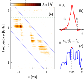
Figure 22: Computing the signal region for the burst 11A.

To choose the optimal value of the tilt $c$, we note that the integral $E_{c}=\int_{\tilde{t}_{1}}^{\tilde{t}_{2}}J_{c}(\tilde{t})\,d\tilde{t}$ estimates the energy within the signal region. We maximize the average signal power ${E_{c}/(\tilde{t}_{2}-\tilde{t}_{1})}$ with respect to $c$ thus choosing the minimal region $t_{1}<t<t_{2}$ with major part of the total energy, see Fig. 22c.

Once the signal region is identified, we perform integrations in Eqs. (1), (2) obtaining the spectral fluence $\bar{F}_{10}(\nu)$. Note that this quantity is computed at all frequencies, even outside of the auxiliary interval $\nu_{1}<\nu<\nu_{2}$. At $\nu<\nu_{1}$ and $\nu>\nu_{2}$ the spectral fluence fluctuates near zero due to noise.

The experimental errors are estimated assuming that the statistical properties of the measuring device are time–independent. For every frequency $\nu$ we select a sufficient number of random time points outside of the signal region, combine the data at these points into an artificial interval $t_{1}(\nu)<t<t_{2}(\nu)$, then use Eqs. (1), (2). This gives the random fluence $\Delta\bar{F}_{10}(\nu)$ of the noise. We finally subtract the statistical mean of $\Delta\bar{F}_{10}$ from Eq. (2) and use its standard deviation to estimate the errors (shaded areas in Fig. 2).

Appendix B Lensing

B.1 Eikonal approximation

In this Appendix we review the effects of plasma and gravitational lenses on the propagating FRB signals. A plasma cloud equips the radio wave with a dispersive phase shift $\varphi_{l}$,

$$\varphi_{l}=-\frac{r_{e}}{\nu}\,\mbox{DM}_{l}(\bm{x})=-\frac{r_{e}}{\nu}\int dz\;\delta n_{e}({\bm{x}},\,z)\;,$$ (B1)

where $\delta n_{e}$ is the overdensity of free electrons, $r_{e}\equiv e^{2}/m_{e}$ is the classical electron radius, and the integral runs along the line of sight. Notably, the dispersive phase Eq. (B1) is inversely proportional to frequency.

We will use the standard (Rickett, 1990; Katz et al., 2020) assumption that the entire dispersive shift Eq. (B1) is acquired on the relatively thin “lens screen” halfway through the plasma cloud, see the dashed line in Fig. 3. This approach explicitly separates the geometric and dispersive effects. It is justified if the lens is spatially separated from the other propagation phenomena.

Now, the dispersive phase Eq. (B1) is a function of the two–coordinate ${\bm{x}}=(x,\,y)$ on the lens screen. Besides, the radio ray $p{\bm{x}}o$ in Fig. 3 consists of two straight parts giving the extra geometric phase shift

$$\phi_{l}=2\pi\nu(r_{p{\bm{x}}}+r_{{\bm{x}}o}-r_{po})\approx({\bm{x}}-\tilde{\bm{x}})^{2}/2r_{F,\,l}^{2}\;.$$ (B2)

Here $r_{p{\bm{x}}}$, $r_{{\bm{x}}o}$, and $r_{po}$ are the distances between the respective points in Fig. 3; in the last equality we used the small–angle approximation $r_{ij}\approx d_{ij}+({\bm{x}}_{i}-{\bm{x}}_{j})^{2}/2d_{ij}$ and collected the total square. Recall that ${\bm{x}}_{p}$ and ${\bm{x}}_{o}$ are the progenitor and observer shifts, $\tilde{\bm{x}}$ is defined in Eq. (4), and $r_{F,\,l}$ is the lens Fresnel scale, see Sec. 3. The total phase shift

$$\Phi_{l}(\bm{x})=\phi_{l}(\bm{x})+\varphi_{l}(\bm{x})$$ (B3)

is the sum of Eqs. (B2) and (B1).

The gravitational lens modifies the phases of radio waves is a different way: by gravitationally attracting the radio rays and changing their length. For convenience we will also divide its phase shift $\Phi_{l}$ into the “naive” geometric part Eq. (B2) and a correction $\varphi_{l}(\bm{x})$ at the “lens screen.” Both $\phi_{l}$ and $\varphi_{l}$ in this case are proportional to the frequency, in contrast to $\nu^{-1}$ behavior of the dispersive shift in Eq. (B1).

The complex amplitude of the observed FRB signal is given by the Fresnel integral

$$f_{\nu}=f_{p}\int\frac{d^{2}{\bm{x}}}{2\pi ir_{F,\,l}^{2}}\;\;\mathrm{e}^{i\Phi_{l}({\bm{x}})}\;,$$ (B4)

where $f_{p}(\nu)$ is the signal of the FRB progenitor.

In this paper we consider lensing in the limit of geometric optics $|{\bm{x}}|\gg r_{F,\,l}$ when the integral (B4) receives main contributions near the stationary points ${\bm{x}}={\bm{x}}_{j}$ of the total phase. These points satisfy the equation,

$${\bm{\nabla}}_{\bm{x}}\Phi_{l}({\bm{x}})\equiv r_{F,\,l}^{-2}({\bm{x}}-\tilde{\bm{x}})+{\bm{\nabla}}_{\bm{x}}\varphi_{l}({\bm{x}})=0\;.$$ (B5)

The signal (B4) is then given by the saddle–point formula,

$$f_{\nu}=f_{p}\sum\limits_{j}\;G_{j}^{1/2}\;\mathrm{e}^{i\Phi_{l}({\bm{x}}_{j})}\;,$$ (B6)

where we introduced the gain factors of the radio paths,

$$G_{j}(\nu)=\Big{|}\det(\delta_{\alpha\beta}+r_{F,\,l}^{2}\partial_{\alpha}\partial_{\beta}\varphi_{l})\Big{|}_{\bm{x}=\bm{x}_{j}}^{-1}$$ (B7)

with ${\partial_{\alpha}\equiv\partial/\partial x_{\alpha}}$. Note that the determinant in Eq. (B7) is not necessarily positive. For convenience we keep $G_{j}>0$ and include the phase of the determinant into ${\Phi_{l}(\bm{x}_{j})\to\Phi_{l}(\bm{x}_{j})-\pi n_{j}/2}$, where $n_{j}=0,1,2$ if $\bm{x}=\bm{x}_{j}$ is a minimum, a saddle point, and a maximum of $\Phi_{l}$, respectively. Once $f_{\nu}$ is computed, one obtains the fluence $F(\nu)\equiv|f_{\nu}|^{2}$.

B.2 Refractive and diffractive lenses

We see that every radio path ${\bm{x}}_{j}$ adds the term ${\Delta F=G_{j}|f_{p}|^{2}}$ to the fluence, while its interference with other paths produces oscillating terms proportional to $\cos(\Phi_{j}-\Phi_{k})$, where $\Phi_{j}\equiv\Phi_{l}({\bm{x}}_{j})$. For example, in the case of two trajectories Eq. (B6) gives,

$$F=F_{p}\left[G_{1}+G_{2}+2(G_{1}G_{2})^{1/2}\;\cos(\Phi_{1}-\Phi_{2})\right]\;,$$ (B8)

with $F\equiv|f_{\nu}|^{2}$ and $F_{p}\equiv|f_{p}|^{2}$ denoting the registered and source fluences, respectively. The last term in Eq. (B8) represents diffraction. As a function of frequency, it oscillates with the period

$$T_{\nu}=2\pi|\partial_{\nu}(\Phi_{1}-\Phi_{2})|^{-1}\sim O(2\pi\nu\,r_{F,\,l}^{2}/a^{2})\;,$$ (B9)

where $a\sim|{\bm{x}}_{2}-\bm{x}_{1}|$ is the typical lens size.

In Sec 3 we consider a refractive lens with extremely large ${a/r_{F,\,l}\gg(\nu/\sigma)^{1/2}}$. In this case the oscillatory term in Eq. (B8) is exponentially dumped by the instrumental smoothing Eq. (1) with window $\sigma$. As a consequence, the main effect of this lens is to multiply the source fluence with the sum of gain factors in Eq. (6).

In Sec. 6 we interpret the periodic spectral structures with $T_{\nu}\sim 100\;\mbox{MHz}$ as the oscillating term in Eq. (B8). Of course, all these structures may be killed by smoothing with sufficiently large window, say, $\sigma=50\;\mbox{MHz}$. In this case $\bar{F}_{50}\approx F_{p}(G_{1}+G_{2})$. The theoretical lens signal Eq. (B8) then can be rewritten as

$$F\approx\bar{F}_{50}\left[1+A_{\mathrm{osc}}\cos(\Phi_{1}-\Phi_{2})\right]\;,$$ (B10)

where

$$A_{\mathrm{osc}}=2(G_{1}G_{2})^{1/2}\;(G_{1}+G_{2})^{-1}\leq 1$$ (B11)

is the relative oscillation amplitude. In the main text we also compute the correlation function Eq. (9) by multiplying $\delta F(\nu)=F-\bar{F}_{50}$ at closeby frequencies $\nu$ and $\nu+\Delta\nu$ and integrating over $\nu$. This procedure exponentially suppresses the terms oscillating with the integration variable $\nu$ leaving

$$\mbox{ACF}(\Delta\nu)=\frac{\cal N}{2}\int\limits_{\nu_{1}}^{\nu_{2}-\Delta\nu}d\nu\;\;\frac{\bar{F}_{50}(\nu)\bar{F}_{50}(\nu+\Delta\nu)}{\nu_{2}-\nu_{1}-\Delta\nu}\\[5.0pt] \times A_{\mathrm{osc}}(\nu)\,A_{\mathrm{osc}}(\nu+\Delta\nu)\,\cos(2\pi\Delta\nu/T_{\nu})\;.$$ (B12)

In the case of narrow–bandwidth spectra with ${\nu_{2}-\nu_{1}\ll\nu}$ and $\Delta\nu\ll\nu$ one can ignore the frequency dependence the period and find,

$$\mbox{ACF}\approx\cos(2\pi\Delta\nu/T_{\nu})\;,$$ (B13)

where the normalization was performed, $\mbox{ACF}(0)=1$. In practice, Eq. (B12) accounts for the wide–band envelope $\bar{F}_{50}$ of the spectrum and therefore better fits the experimental data, though Eq. (B13) is simpler and may be used on preparatory stages.

B.3 Gaussian overdensity lens

In Sec. 3 we consider a Gaussian lens with the profile ${\varphi_{l}=-(r_{e}/\nu)\,\mbox{DM}_{l}\,\mathrm{e}^{-x^{2}/a^{2}}}$ depending only on one transverse coordinate $x$. The total phase shift Eqs. (B2), (B3) in this case reduces to Eq. (3). The $y$ component of the eikonal equation (B5) gives $y_{j}=\tilde{y}$ implying that the lens bends the radio waves only in the $x$ direction. The other, $x$ component, has the form

$$f(u)\equiv u-\tilde{u}+\alpha u\mathrm{e}^{-u^{2}}=0\;,$$ (B14)

where $u=x/a$ and $\tilde{u}=\tilde{x}/a$. We denote the solutions of this equation by $u_{j}$. The net gain factor Eq. (6) equals $G(\nu)=\sum_{j}|\partial_{u}f(u_{j})|^{-1}$.

Let us show that the lens caustics — solutions $u_{*}$ of Eq. (B14) with infinite gain factor $G$ — exist only if $\tilde{x}/a=\tilde{u}$ exceeds the critical value $\tilde{u}_{\mathrm{cr}}=(3/2)^{3/2}$. Indeed, by definition $u_{*}$ satisfy equations $f(u_{*})={\partial_{u}f(u_{*})=0}$ which can be written in the form ${\alpha_{l}=\mathrm{e}^{u_{*}^{2}}/(2u_{*}^{2}-1)}$ and $\tilde{u}=2u_{*}^{3}/(2u_{*}^{2}-1)$. The right–hand side of the last equation is bounded from below by the global minimum $\tilde{u}\geq\tilde{u}_{\mathrm{cr}}$ which occurs at $u_{*}=u_{\mathrm{cr}}\equiv\sqrt{3/2}$ and $\alpha_{l}=\alpha_{\mathrm{cr}}\equiv\frac{1}{2}\mathrm{e}^{3/2}$. We conclude that the lens caustics exist only for overcritical lens shifts, $\tilde{u}\geq\tilde{u}_{\mathrm{cr}}$. At $\tilde{u}=\tilde{u}_{\mathrm{cr}}$ they appear at the critical “frequency” $\alpha_{l}^{-1/2}=\alpha_{\mathrm{cr}}^{-1/2}$ and move apart as $\tilde{u}$ grows.

Consider the near–critical situation when $\tilde{u}$ slightly exceeds $\tilde{u}_{\mathrm{cr}}$. This corresponds to a nearby pair of caustics in the lens spectrum with $\alpha_{*\pm}$ and $u_{*\pm}$ close to $\alpha_{\mathrm{cr}}$ and $u_{\mathrm{cr}}$. Performing the Taylor series expansion in $u-u_{\mathrm{cr}}$ and $\alpha_{l}-\alpha_{\mathrm{cr}}$, we rewrite the lens equation as

$$f\approx\tilde{u}_{\mathrm{cr}}-\tilde{u}-(\alpha_{l}/\alpha_{\mathrm{cr}}-1)(u-3u_{\mathrm{cr}}/2)\\ +(u-u_{\mathrm{cr}})^{3}=0\;.$$ (B15)

Now, we can explicitly solve the caustic equations $f(u_{*})=\partial_{u}f(u_{*})=0$ with respect to $u_{*}$ and “frequency” $\alpha_{l}$ finding

$$u_{*\,\pm}\approx u_{\mathrm{cr}}\pm\frac{1}{\sqrt{3}}(\alpha_{*\,\pm}/\alpha_{\mathrm{cr}}-1)^{1/2}\;,$$ (B16)

$$\alpha_{*\,{\pm}}\approx\alpha_{\mathrm{cr}}\left[3\tilde{u}/\tilde{u}_{\mathrm{cr}}-2\pm\frac{4}{u_{\mathrm{cr}}}\,\left(\tilde{u}/\tilde{u}_{\mathrm{cr}}-1\right)^{3/2}\right]\;,$$ (B17)

where expansion in $\tilde{u}-\tilde{u}_{\mathrm{cr}}$ was performed, again. Since $\alpha_{l}\propto\nu^{-2}$, the last expression fixes the positions of caustics $\nu_{0}\pm\Delta\nu$ of the lens spectrum: $\alpha_{l}(\nu_{0})=(\alpha_{*\,+}+\alpha_{*\,-})/2$ and $\Delta\nu/\nu_{0}=|\alpha_{*\,+}-\alpha_{*\,-}|/2\alpha_{\mathrm{cr}}$. We obtain,

$$\tilde{u}\approx\tilde{u}_{\mathrm{cr}}+\tilde{u}_{\mathrm{cr}}\left(\frac{\Delta\nu\sqrt{3}}{4\nu_{0}\sqrt{2}}\right)^{2/3}\;,$$ (B18)

$$\alpha_{l}(\nu_{0})\approx\alpha_{\mathrm{cr}}\left(3\tilde{u}/\tilde{u}_{\mathrm{cr}}-2\right)\;.$$ (B19)

In the main text these expressions are used to compute $\tilde{u}=\tilde{x}/a$ and $\beta$.

Now, suppose the lens shift $\tilde{u}$ is slightly below $\tilde{u}_{\mathrm{cr}}$. In this case Eq. (B15) has only one solution $u=u_{1}$, and the gain factor $G=[3(u_{1}-u_{\mathrm{cr}})^{2}+1-\alpha_{l}/\alpha_{\mathrm{cr}}]^{-1}$ is smooth. Nevertheless, $G(u_{1})$ has a sharp maximum at $u_{1}=u_{\mathrm{cr}}$. Half–height of the maximum is reached at $u_{1}-u_{\mathrm{cr}}=\pm\frac{1}{\sqrt{3}}(1-\alpha_{l}/\alpha_{\mathrm{cr}})^{1/2}$. Substituting these points into Eq. (B15), we find the “frequency” of the maximum $\alpha_{l}=\alpha_{l}(\nu_{0})$ and its half–height width ${\Delta\nu^{\prime}/\nu_{0}=\Delta\alpha_{l}/2\alpha_{\mathrm{cr}}}$,

$$\tilde{u}\approx\tilde{u}_{\mathrm{cr}}-\tilde{u}_{\mathrm{cr}}\left(\frac{\Delta\nu^{\prime}\sqrt{3}}{8\nu_{0}\sqrt{2}}\right)^{2/3}\;,$$ (B20)

$$\alpha_{l}(\nu_{0})\approx\alpha_{\mathrm{cr}}\left(3\tilde{u}/\tilde{u}_{\mathrm{cr}}-2\right)\;.$$ (B21)

These equations relate the “main” spectral peak to the parameters of the lens with $\tilde{x}<\tilde{x}_{\mathrm{cr}}$.

It is worth reminding that the analytic treatment of this Appendix is applicable for narrow lens spectra, $\Delta\nu/\nu_{0}\ll 1$. Notably, in this case the two– or one–peaked lens contributions are easily recognizable on the experimental graphs.

B.4 Diffractive underdensity lens

In Sec. 6 we study diffraction of radio rays splitted by the plasma lens. We use the same Gaussian profile of the dispersive phase shift $\varphi_{l}$ as before, but with different sign in front of it, see Eq. (20). This lens describes a hole in the interstellar plasma, i.e. an underdensity of free electrons: ${\alpha_{l}^{\prime}\propto-\delta n>0}$.

The lens Eq. (20) has too many parameters and easily fits the experimental data, so in the main text we voluntarily choose the simplest and most illustrative regime: strong lens relatively far away from the line of sight, $\ln\alpha_{l}^{\prime}\gg 1$ and $\tilde{x}^{\prime}/a^{\prime}\sim\sqrt{\ln\alpha_{l}^{\prime}}$. Then the eikonal equation (B5), (20) gives three rays, cf. Fig. 20,

$$x_{1,2}\approx\pm a^{\prime}\sqrt{\ln\alpha_{l}^{\prime}}\;,\qquad x_{3}\approx-\tilde{x}/\alpha_{l}^{\prime}\;,$$ (B22)

where corrections to $x_{1,2}$ are suppressed by $(\ln\alpha_{l}^{\prime})^{-1}$. Recall that the one–dimensional lens does not bend the rays in the $y$ direction: $y_{j}=\tilde{y}^{\prime}$. Plugging the eikonal equation into Eq. (B7), we simplify the expression for the lens gain factor: $G=|2x^{2}/a^{\prime 2}-2x\tilde{x}^{\prime}/a^{\prime 2}+\tilde{x}^{\prime}/x|^{-1}$. Three solutions (B22) then give,

$$G_{1,2}\approx\frac{1}{2\ln\alpha_{l}^{\prime}}\left(1\mp\frac{\tilde{x}^{\prime}}{a^{\prime}\sqrt{\ln\alpha_{l}^{\prime}}}\right)^{-1}\;,\;\;G_{3}\approx\frac{1}{\alpha_{l}^{\prime}}\;.$$ (B23)

Notably, in our regime $\ln\alpha_{l}^{\prime}\gg 1$ the contribution of the third radio path can be ignored and we obtain the two–wave interference in Eq. (16).

Computing the phases Eq. (20) of the two remaining solutions, we obtain,

$$\Phi_{2}-\Phi_{1}\approx 2a^{\prime}\tilde{x}^{\prime}\sqrt{\ln\alpha_{l}^{\prime}}/r_{F,\,l}^{\prime 2}\;.$$ (B24)

Now, the expressions (B9) and (B11) give the frequency period $T_{\nu}$ and relative amplitude $A_{\mathrm{osc}}$ of the interference oscillations. We derived Eqs. (21) from the main text.

B.5 Gravitational lens

In the main text we speculate that the periodic spectral structure may be explained by gravitational lensing of the FRB signals on a compact object hiding at distance $d_{lo}^{\prime}$ from us. A phase shift of the radio waves in the gravitational field of a point–like lens is given by Eq. (22), see also Peterson & Falk (1991), Matsunaga & Yamamoto (2006), Bartelmann (2010), Katz et al. (2020). The latter expression still has the form (B3), (B2), like in the case of refraction, but with a specific $\varphi_{l}$ term. We treat the gravitational lens in the same eikonal approximation as before.

The lens equation (B5) has two solutions,

$$\bm{x}_{1,\,2}=\bm{x}_{o}+\frac{1}{2}\,\theta_{E}\,d_{lo}^{\prime}\,\bm{\zeta}\left(1\pm\sqrt{1+4\bm{\zeta}^{-2}}\right)\;,$$ (B25)

where we introduced the vector $\bm{\zeta}=(\bm{x}_{p}-\bm{x}_{o})/(d_{po}\theta_{E})$ characterizing the angular shift of the source from the lens in units of $\theta_{E}$. Equations (B7) and (22) give,

$$G_{1,2}=\frac{\zeta^{2}+2}{2\zeta\sqrt{\zeta^{2}+4}}\pm\frac{1}{2}\;,$$

$$\Phi_{2}-\Phi_{1}=\Omega\left[\zeta\sqrt{\zeta^{2}+4}+2\ln(\zeta/2+\sqrt{\zeta^{2}/4+1})\right]-\frac{\pi}{2},$$

where $\zeta\equiv|\bm{\zeta}|$ an we denoted $\Omega=8\pi\nu GM$. Using finally Eqs. (B11) and (B9), we obtain the parameters of spectral oscillations in Eq. (23) of the main text.

Appendix C Scintillations $+$ lensing

C.1 Adding the scintillation screen

In practice regular structures coexist in the FRB spectra with random scintillations caused by refraction of radio waves in the turbulent interstellar clouds. To describe the latter effect theoretically, we add a thin transverse “scintillation” screen that equips any propagating wave with a random phase $\varphi_{S}({\bm{\xi}})$, where ${{\bm{\xi}}=(\xi_{x},\,\xi_{y})}$ is a two–coordinate on the screen, see Fig. 13. For definiteness, we assume that the scintillations occur between the lens and the observer at distances $d_{lS}$ and $d_{So}$; we will comment on the other choice below. Physically, the scintillations may happen in the FRB host galaxy and / or the Milky Way.

Since the scintillation phase $\varphi_{S}$ is caused by refraction, it is given by Eq. (B1). But now $\delta n_{e}$ is a random component of the electron overdensity. It is customary to assume that this component has a homogeneous and isotropic Kolmogorov turbulent spectrum, see Cordes et al. (1985), Rickett (1990), Narayan (1992), Lorimer & Kramer (2004), Woan (2011), Katz et al. (2020):

$$\langle\delta n_{e}(\bm{X})\,\delta n_{e}(\bm{X}^{\prime})\rangle\\ =C_{n}^{2}\int_{\kappa_{\mathrm{out}}}^{\kappa_{in}}d^{3}\bm{\kappa}\;|\bm{\kappa}|^{-11/3}\;\mathrm{e}^{i\bm{\kappa}(\bm{X}^{\prime}-\bm{X})}\;,$$ (C1)

where $\bm{X}$ and $\bm{X}^{\prime}$ represent the three–dimensional space coordinates and $\kappa_{\mathrm{in}}\gg\kappa_{\mathrm{out}}$ — the cutoff scales for turbulence. Angular brackets in Eq. (C1) average over realizations of the turbulent ensemble e.g. volumes within the galaxy. Using Eq. (B1), one can turn Eq. (C1) into a correlator of two $\varphi_{S}$’s (Rickett, 1990; Katz et al., 2020),

$$S_{\nu}(\bm{\xi}-\bm{\xi}^{\prime})\equiv\langle\left[\varphi_{S}(\bm{\xi})-\varphi_{S}(\bm{\xi}^{\prime})\right]^{2}\rangle=\frac{|\bm{\xi}-\bm{\xi}^{\prime}|^{5/3}}{r_{\mathrm{diff}}^{5/3}}\;,$$ (C2)

where we introduced the diffractive length scale

$$r_{\mathrm{diff}}=3.63\cdot 10^{10}\,\mbox{cm}\,\left(\frac{C_{n}^{2}\cdot L}{10^{-4}\,\mbox{m}^{-20/3}\cdot\mbox{kpc}}\right)^{-3/5}\\ \times\left(\frac{\nu}{6\,\mbox{GHz}}\right)^{6/5}\;,$$ (C3)

and thickness of the scintillation screen $L\sim\mbox{kpc}$. Equation (C2) implies that the rays crossing the screen at distance $r_{\mathrm{diff}}$ receive relative random phases of order 1. This makes them incoherent at $|\bm{\xi}-\bm{\xi}^{\prime}|\gtrsim r_{\mathrm{diff}}$. Technically, it will be important for us that the correlator Eq. (C2) is translationally invariant, i.e. depends on $|\bm{\xi}-\bm{\xi}^{\prime}|$, and proportional to $\nu^{-2}$, cf. Eq. (B1).

In this Appendix we describe the scintillations statistically i.e. compute the mean FRB spectra and their correlation functions. Recall that in the main text we average the experimental data over the frequency relying on the fact that they become statistically independent if $\nu$ is shifted by $\nu_{d}$ — the decorrelation bandwidth. This approach is applicable for narrow–band scintillations of Sec. 5 that have small $\nu_{d}$ compared to the total FRB bandwidth $\nu_{\mathrm{bw}}\sim\mbox{GHz}$. The same description is at best qualitative, however, in the case of wide–band scintillations considered in Sec. 4. Below we heavily rely on the expansion in ${\nu_{d}/\nu\ll 1}$.

In the thin–screen approach of Fig. 13 the radio ray $p\bm{x\xi}o$ consists of three straight parts. Its geometric phase shift can be written as

$$\phi=\phi_{l}(\bm{x})+\phi_{S}(\bm{x},\,\bm{\xi})\;,$$ (C4)

where $\phi_{l}$ is the same lens shift Eq. (B2) as before and

$$\phi_{S}=2\pi\nu(r_{\bm{x}\bm{\xi}}+r_{\bm{\xi}o}-r_{\bm{x}o})\approx(\bm{\xi}-\tilde{\bm{\xi}})^{2}/2r_{F,\,S}^{2}$$ (C5)

accounts for the additional turn at the point $\bm{\xi}$ of the scintillation screen. We introduced the coordinate

$$\tilde{\bm{\xi}}(\bm{x})=(d_{So}\bm{x}+d_{lS}\bm{x}_{o})/d_{lo}$$ (C6)

corresponding to straight propagation between $\bm{x}$ and $o$. Besides,

$$r_{F,\,S}=(d_{lS}d_{So}/2\pi\nu d_{lo})^{1/2}$$ (C7)

is the Fresnel scale for scintillations.

To sum up, we consider radio wave which sequentially crosses the lens and the scintillating medium acquiring the total phase $\Phi=\phi_{l}+\varphi_{l}+\phi_{S}+\varphi_{S}$. The Fresnel integral for this wave has the form, cf. Eq. (B4),

$$f_{\nu}=f_{p}\int\frac{d^{2}\bm{x}}{{2\pi ir_{F,\,l}^{2}}}\;\;\mathrm{e}^{i\phi_{l}(\bm{x})+i\varphi_{l}(\bm{x})}\;{\cal A}_{\nu}(\bm{x})\;,$$ (C8)

where the new factor ${\cal A}_{\nu}$ in the integrand accounts for scintillations,

$${\cal A}_{\nu}=\int\frac{d^{2}\bm{\xi}}{2\pi ir_{F,\,S}^{2}}\;\;\mathrm{e}^{i\phi_{S}(\bm{x},\,\bm{\xi})+i\varphi_{S}(\bm{\xi})}\;.$$ (C9)

Recall that $\varphi_{S}$ and hence $f_{\nu}$ are the random quantities.

C.2 Mean fluence

The Fresnel integral for the averaged fluence ${\langle F\rangle=\langle f_{\nu}f_{\nu}^{*}\rangle}$ runs over $\bm{x},\;\bm{\xi}$ and $\bm{x}^{\prime},\;\bm{\xi}^{\prime}$ which come from the integrals (C8), (C9) for $f_{\nu}$ and $f_{\nu}^{*}$, respectively. In this expression, the statistical mean $\langle\cdot\rangle$ acts on the random phase ${\exp[i\varphi_{S}(\bm{\xi})-i\varphi_{S}(\bm{\xi}^{\prime})]}$ in the integrand. Recall that we consider weakly interacting turbulent plasma with $\varphi_{S}\propto\delta n_{e}$ behaving as a Gaussian random quantity. Any correlator of such quantity can be computed in terms of the two–point function (C2). In particular,

$$\langle\mathrm{e}^{i\varphi_{S}(\bm{\xi})-i\varphi_{S}(\bm{\xi}^{\prime})}\rangle=\mathrm{e}^{-S_{\nu}(\bm{\xi}-\bm{\xi}^{\prime})/2}\;.$$ (C10)

Thus, the scintillation factor in the integrand of $\langle F\rangle$ equals,

$$\langle{\cal A}_{\nu}{\cal A}_{\nu}^{\prime*}\rangle=\int\frac{d^{2}\bm{\xi}\,d^{2}\bm{\xi}^{\prime}}{4\pi^{2}r_{F,\,S}^{4}}\;\;\mathrm{e}^{i\phi_{S}(\bm{x},\,\bm{\xi})-i\phi_{S}(\bm{x}^{\prime},\,\bm{\xi}^{\prime})-S_{\nu}(\bm{\xi}-\bm{\xi}^{\prime})/2}\;,$$

where ${\cal A}_{\nu}^{\prime}\equiv{\cal A}_{\nu}(\bm{x}^{\prime})$. From Eq. (C5) one learns that $\bm{\xi}+\bm{\xi}^{\prime}$ enters linearly the exponent. As a consequence, the integral over this combination produces ${\delta^{(2)}[\bm{\xi}-\bm{\xi}^{\prime}-\tilde{\bm{\xi}}(\bm{x})+\tilde{\bm{\xi}}(\bm{x}^{\prime})]}$, and we obtain,

$$\langle{\cal A}_{\nu}{\cal A}_{\nu}^{\prime*}\rangle=\exp\left(-\frac{|\bm{x}-\bm{x}^{\prime}|^{5/3}}{2\tilde{r}_{\mathrm{diff}}^{5/3}}\right)\;,$$ (C11)

where a projection

$$\tilde{r}_{\mathrm{diff}}=d_{lo}r_{\mathrm{diff}}/d_{So}$$ (C12)

of the diffractive scale onto the lens screen was introduced.

We conclude that the net effect of scintillations is to ruin coherence in $\langle F\rangle$ i.e. suppress contributions of radio paths $\bm{x}$ and $\bm{x}^{\prime}$ if the distance between them exceeds $\tilde{r}_{\mathrm{diff}}$. Using Eqs. (C8), (C11), we write the mean fluence as

$$\langle F\rangle=F_{p}\int\frac{d\bm{x}d\bm{x}^{\prime}}{4\pi^{2}r_{F,\,l}^{4}}\,\mathrm{e}^{i\Phi_{l}-i\Phi_{l}^{\prime}-\frac{1}{2}(|\bm{x}-\bm{x}^{\prime}|/\tilde{r}_{\mathrm{diff}})^{5/3}}\;,$$ (C13)

where $F_{p}\equiv|f_{p}|^{2}$, $\Phi_{l}\equiv\phi_{l}(\bm{x})+\varphi_{l}(\bm{x})$, and $\Phi_{l}^{\prime}\equiv\Phi_{l}(\bm{x}^{\prime})$. Note that the lens lurking in the FRB host galaxy is almost insensitive to the scintillations in the Milky Way: $\tilde{r}_{\mathrm{diff}}/r_{\mathrm{diff}}=d_{lo}/d_{So}\sim 10^{6}$.

If the scintillations occur between the source and the lens, the integral (C13) is still valid but the projected diffractive scale equals $\tilde{r}_{\mathrm{diff}}=d_{pl}r_{\mathrm{diff}}/d_{pS}$. Then the scintillations in the FRB host galaxy are geometrically suppressed if the lens is near us.

Now, recall that we consider large–size lenses in the limit of geometric optics $\Phi_{l}\gg 1$, cf. Appendix B. At the same time, we are interested in detectably large contributions i.e. in the situation when the scintillation factor is not too small i.e. ${|\bm{x}-\bm{x}^{\prime}|/\tilde{r}_{\mathrm{diff}}\lesssim\mbox{few}}$. In this case the integral is dominated by the same stationary points $\bm{x}=\bm{x}_{j}$ and $\bm{x}^{\prime}=\bm{x}_{j^{\prime}}$ — the paths of radio rays — as in the case without the scintillations. We obtain,

$$\langle F\rangle=F_{p}\sum\limits_{jj^{\prime}}(G_{j}G_{j^{\prime}})^{1/2}\,\mathrm{e}^{i\Phi_{l}(\bm{x}_{j})-i\Phi_{l}(\bm{x}_{j^{\prime}})}\\ \times\mathrm{e}^{-\frac{1}{2}(|\bm{x}_{j}-\bm{x}_{j^{\prime}}|/\tilde{r}_{\mathrm{diff}})^{5/3}}$$ (C14)

where $\bm{x}_{j}$ solve the lens equation (B5) and the gain factors $G_{j}$ are given by the same determinant as before. The effect of the scintillations is represented by the exponent in the second line of Eq. (C14).

In the simplified case of two radio paths one obtains the analog of Eq. (B10),

$$\langle F\rangle=\bar{F}_{50}\Big{[}1+A_{\mathrm{osc}}\;\mathrm{e}^{-\frac{1}{2}(|\bm{x}_{1}-\bm{x}_{2}|/\tilde{r}_{\mathrm{diff}})^{5/3}}\cos(\Phi_{1}-\Phi_{2})\Big{]}\;,$$ (C15)

where the only new factor is a scintillating exponent suppressing interference between the trajectories with $|\bm{x}_{1}-\bm{x}_{2}|\gtrsim\tilde{r}_{\mathrm{diff}}$. Note that it is hard to compare Eq. (C15) with experiment. We already explained that the only practical way to perform the statistical average is to smooth over frequency. But — alas — the same procedure kills the oscillating interference terms. Thus, one either has to consider sophisticated statistical methods like Kolmogorov–Smirnov–Kuiper test (Press et al., 2007) or analyze more involved spectral correlators.

C.3 Autocorrelation function

Now, consider the mean product of fluences at nearby frequencies $\nu$ and $\nu_{1}=\nu+\Delta\nu$,

$$\langle F(\nu)F(\nu_{1})\rangle=\langle f_{\nu}f_{\nu}^{*}f_{\nu_{1}}f_{\nu_{1}}^{*}\rangle\;.$$ (C16)

Using Eqs. (C8), (C9) for the amplitudes, we write it in the form of a Fresnel integral over $(\bm{x},\;\bm{\xi})$, $(\bm{x}^{\prime},\;\bm{\xi}^{\prime})$, $(\bm{x}_{1},\;\bm{\xi}_{1})$, and $(\bm{x}_{1}^{\prime},\;\bm{\xi}_{1}^{\prime})$. Here and below we mark all quantities related to the last three amplitudes $f_{\nu}^{*}$, $f_{\nu_{1}}$, and $f_{\nu_{1}}^{*}$ by prime, 1, and 1-prime, respectively.

     

Figure 23: Two graphical representations of Eq. (C18).

The integrand of the above four–wise Fresnel integral involves a statistical average of four random phases

$$\mathrm{e}^{-S_{4}/2}\equiv\langle\mathrm{e}^{i\varphi_{S}-i\varphi_{S}^{\prime}+i\varphi_{S1}-i\varphi_{S1}^{\prime}}\rangle\;,$$ (C17)

where $\varphi_{S1}^{\prime}\equiv\varphi_{S}(\bm{\xi}_{1}^{\prime})$, etc. Like before, this correlator can be computed by recalling that $\varphi_{S}$ is a Gaussian random variable and exploiting Eq. (C2),

$$S_{4}= \langle\left(\varphi_{S}-\varphi_{S}^{\prime}+\varphi_{S1}-\varphi_{S1}^{\prime}\right)^{2}\rangle$$ (C18)

$$= S_{\nu}(\bm{\xi}-\bm{\xi}^{\prime})+\frac{\nu^{2}}{\nu_{1}^{2}}\;S_{\nu}(\bm{\xi}_{1}-\bm{\xi}_{1}^{\prime})+\frac{\nu}{\nu_{1}}S_{\nu}(\bm{\xi}_{1}^{\prime}-\bm{\xi})$$

$$+\frac{\nu}{\nu_{1}}\Big{[}S_{\nu}(\bm{\xi}_{1}-\bm{\xi}^{\prime})-S_{\nu}(\bm{\xi}_{1}-\bm{\xi})-S_{\nu}(\bm{\xi}_{1}^{\prime}-\bm{\xi}^{\prime})\Big{]}\;,$$

where we explicitly used the fact that $\varphi_{S}\propto\nu^{-1}$, cf. Eq. (B1). Expression (C18) looks complicated. That is why we visualize it in Fig. 23 by drawing every $S_{\nu}(\bm{\xi}-\bm{\xi}^{\prime})$ with an “attractive” spring between $\bm{\xi}$ and $\bm{\xi}^{\prime}$, and $(-S_{\nu})$ — with a “repulsive” solid line.

The exponent (C17) cuts off the $\bm{\xi}$ integrations in regions with large $S_{4}$. Generically, this happens if the distances between $\bm{\xi}$’s exceed $r_{\mathrm{diff}}$. However, there are two valleys — large integration regions with small $S_{4}$. First, one can keep $(\bm{\xi},\;\bm{\xi}^{\prime})$ and $(\bm{\xi}_{1},\,\bm{\xi}_{1}^{\prime})$ in tight pairs increasing the distance $\bm{R}=\bm{\xi}_{1}-\bm{\xi}$ between them, see “Valley I” in Fig. 23a. In this case

$$S_{4}\big{|}_{\mathrm{valley}\;\mathrm{I}}\approx S_{\nu}(\bm{\xi}-\bm{\xi}^{\prime})+S_{\nu_{1}}(\bm{\xi}_{1}-\bm{\xi}_{1}^{\prime})\;,$$ (C19)

with corrections of order $(r_{\mathrm{diff}}/|\bm{R}|)^{1/3}$. Second, we can move apart the pairs $(\bm{\xi},\,\bm{\xi}_{1}^{\prime})$ and $(\bm{\xi}_{1},\,\bm{\xi}^{\prime})$ in Fig. 23b. This gives

$$S_{4}\big{|}_{\mathrm{valley}\;\mathrm{II}}\approx(\Delta\nu/\nu)^{2}\,S_{\nu}(\bm{\xi}_{1}-\bm{\xi})+S_{\nu}(\bm{\xi}-\bm{\xi}_{1}^{\prime})\\ +S_{\nu}(\bm{\xi}_{1}-\bm{\xi}^{\prime})\;,$$ (C20)

with $\Delta\nu\equiv\nu_{1}-\nu$ and similar corrections as before. Soon we will see that $(r_{\mathrm{diff}}/R)^{1/3}\sim(\nu_{d}/\nu)^{1/3}\sim 8\%$, where the numerical estimate is performed for narrow–band scintillations of Sec. 5.

Now, consider the scintillation factor ${{\cal A}_{4}\equiv\langle{\cal A}_{\nu}{\cal A}_{\nu}^{\prime*}{\cal A}_{\nu_{1}}{\cal A}_{\nu_{1}}^{\prime*}\rangle}$ in the Fresnel integral for Eq. (C16). It involves four $\bm{\xi}$–integrals,

$${\cal A}_{4}=\int\frac{d^{2}\{\bm{\xi}\bm{\xi^{\prime}}\bm{\xi}_{1}\bm{\xi}_{1}^{\prime}\}}{(2\pi r_{F,\,S}^{2})^{4}}\;\;\mathrm{e}^{i\phi_{S}-i\phi_{S}^{\prime}+i\phi_{S1}-i\phi_{S1}^{\prime}-S_{4}/2}\;,$$ (C21)

see Eq. (C9). Valleys I and II with paired $\bm{\xi}$’s give major contributions into ${\cal A}_{4}$. From the technical viewpoint, these valleys appear because the four scintillation factors correlate in pairs and their average product almost equals the sum of $\langle{\cal A}_{\nu}{\cal A}_{\nu}^{\prime*}\rangle\langle{\cal A}_{\nu_{1}}{\cal A}_{\nu_{1}}^{\prime*}\rangle$ and $\langle{\cal A}_{\nu}{\cal A}_{\nu_{1}}^{\prime*}\rangle\langle{\cal A}_{\nu_{1}}{\cal A}_{\nu}^{\prime*}\rangle$, with two–point correlators decaying exponentially at far–away $\bm{\xi}$’s.

Let us start with the valley I, Eq. (C19). In this case the averaged scintillation phase $\exp(-S_{4}/2)$ depends separately on $(\bm{\xi},\,\bm{\xi}^{\prime})$ and $(\bm{\xi}_{1},\,\bm{\xi}_{1}^{\prime})$. Integrating over these pairs in the same way as in Sec. C.2, we find,

$${\cal A}_{4}\big{|}_{\mathrm{valley}\;\mathrm{I}}\approx\mathrm{e}^{-\frac{1}{2}(|\bm{x}-\bm{x}^{\prime}|/\tilde{r}_{\mathrm{diff}})^{5/3}-\frac{1}{2}(|\bm{x}_{1}-\bm{x}_{1}^{\prime}|/\tilde{r}_{\mathrm{diff}})^{5/3}}\!,$$ (C22)

where $\tilde{r}_{\mathrm{diff}}$ is the projected diffraction scale Eq. (C12). Due to Eq. (C22), the entire correlator Eq. (C16) factorizes along valley I into

$$\langle F(\nu)F(\nu_{1})\rangle\big{|}_{\mathrm{valley}\;\mathrm{I}}\approx\langle F(\nu)\rangle\langle F(\nu_{1})\rangle\;,$$ (C23)

cf. Eq. (C13).

The valley II is a bit different. The exponent $S_{4}$ in Eq. (C20) weakly depends on the variable ${\bm{R}\equiv\bm{\xi}_{1}-\bm{\xi}}$ along this valley because the random phases do not completely compensate in the products ${\cal A}_{\nu}{\cal A}_{\nu_{1}}^{\prime*}$ and ${\cal A}_{\nu_{1}}{\cal A}_{\nu}^{\prime*}$ at $\nu_{1}\neq\nu$. Nevertheless, we will see that the $\bm{R}$–dependence factorizes: the factor $(\Delta\nu/\nu)^{2}\ll 1$ in front of the first term in Eq. (C20) makes it insensitive to the small displacements $\delta\bm{\xi}=\bm{\xi}-\bm{\xi}_{1}^{\prime}$ and $\delta\bm{\xi}_{1}=\bm{\xi}_{1}-\bm{\xi}^{\prime}$ transverse to the valley. Indeed, notice that due to the shift symmetry the center–of–mass variable $\bm{\xi}+\bm{\xi}^{\prime}+\bm{\xi}_{1}+\bm{\xi}_{1}^{\prime}$ enters linearly in the exponent of Eq. (C21) and therefore gives

$$\delta^{(2)}\left[\bm{R}-\tilde{\bm{R}}+\frac{\nu}{\Delta\nu}\,(\delta\bm{\xi}+\delta\bm{\xi}_{1}-\delta\tilde{\bm{\xi}}-\delta\tilde{\bm{\xi}}_{1})\right]\;,$$

where we introduced $\tilde{\bm{R}}=\tilde{\bm{\xi}}_{1}-\tilde{\bm{\xi}}$, $\delta\tilde{\bm{\xi}}=\tilde{\bm{\xi}}-\tilde{\bm{\xi}}_{1}^{\prime}$, etc., like in the case without the tildes. This fixes the value of $\bm{R}$ leaving only the integrals over $\delta\bm{\xi}$ and $\delta\bm{\xi}_{1}$ in Eq. (C21). Notably, $\delta\bm{\xi},\;\delta\bm{\xi}_{1}\sim r_{\mathrm{diff}}$, and thus ${|\bm{R}|/r_{\mathrm{diff}}\sim\nu/\Delta\nu\sim\nu/\nu_{d}}$, like was announced previously. Moreover, we indeed can use $\bm{R}\approx\tilde{\bm{R}}\equiv(\bm{x}_{1}-\bm{x})d_{So}/d_{lo}$ in the first term of Eq. (C21) ignoring corrections because this term is already suppressed by the factor $(\Delta\nu/\nu)^{2}$.

Once this is done, dependences on $\delta\bm{\xi}$ and $\delta\bm{\xi}_{1}$ factorize and we arrive to

$${\cal A}_{4}\big{|}_{\mathrm{valley}\;\mathrm{II}}=\exp\left\{-\frac{\Delta\nu^{2}}{2\nu^{2}}\,\frac{|\bm{x}-\bm{x}_{1}|^{5/3}}{\tilde{r}_{\mathrm{diff}}^{5/3}}\right\}\\ \times{\cal J}_{\Delta\nu}\left(\frac{|\bm{x}-\bm{x}_{1}^{\prime}|}{\tilde{r}_{\mathrm{diff}}}\right)\;{\cal J}_{\Delta\nu}^{*}\left(\frac{|\bm{x}_{1}-\bm{x}^{\prime}|}{\tilde{r}_{\mathrm{diff}}}\right)\;,$$ (C24)

where the functions ${\cal J}_{\Delta\nu}(\rho)$ and ${\cal J}^{*}_{\Delta\nu}(\rho_{1})$ include integrals over $\delta\bm{\xi}$ and $\delta\bm{\xi}_{1}$. The latter can be written in the simplified form

$${\cal J}_{\Delta\nu}(\rho)=-i\,\mathrm{e}^{i\rho^{2}/w}\\ \times\int_{0}^{\infty}d\zeta\;\mathrm{e}^{i\zeta-\frac{1}{2}(w\zeta)^{5/6}}J_{0}\left(2\rho\sqrt{\zeta/w}\right)\;.$$ (C25)

We introduced the rescaled frequency lag $w\equiv 2\Delta\nu/\nu_{d}$, decorrelation bandwidth ${\nu_{d}\equiv\nu\,(r_{\mathrm{diff}}/r_{F,\,S})^{2}}$, the argument $\rho$ is of ${\cal J}_{\Delta\nu}$ measuring distances between $\bm{x}$’s in units of $\tilde{r}_{\mathrm{diff}}$, and the Bessel function $J_{0}$. Note that the ${\cal J}$–factors in Eq. (C24) do the same job as the exponent in Eq. (C22): they force $|\bm{x}-\bm{x}_{1}^{\prime}|$ and $|\bm{x}_{1}-\bm{x}^{\prime}|$ to be smaller than $\tilde{r}_{\mathrm{diff}}$. Indeed, ${\cal J}_{\Delta\nu}(\rho)\to\exp\{-\frac{1}{2}\rho^{5/3}\}$ as $\rho\to+\infty$. At $\rho\lesssim w$ this function remains unsuppressed and essentially depends on the frequency lag $w\propto\Delta\nu$.

We finally consider the integrals over the lensed radio paths $\bm{x}$, $\bm{x}^{\prime}$, $\bm{x}_{1}$, and $\bm{x}_{1}^{\prime}$ in the Fresnel representation of the correlator Eq. (C16), cf. Eq. (C8). The scintillations supply the factor in the integrand,

$${\cal A}_{4}(\bm{x},\,\bm{x}^{\prime},\,\bm{x}_{1},\,\bm{x}_{1}^{\prime})={\cal A}_{4}\big{|}_{\mathrm{valley}\;\mathrm{I}}+{\cal A}_{4}\big{|}_{\mathrm{valley}\;\mathrm{II}}\;,$$ (C26)

given by the sum of Eqs. (C22) and (C24).

Like in the previous Sections, we consider only large–size lenses in the limit of geometric optics. In this case the phase shift is large, ${\Phi_{l}\sim|\bm{x}-\tilde{\bm{x}}|^{2}/r_{F,\,l}^{2}\gg 1}$, and the Fresnel integral is dominated by the set of distinguished rays $\{\bm{x}_{j}\}$ satisfying the lens equation (B5). Notably, one can roughly estimate the typical lens phase via Eq. (B9) obtaining $\Phi_{l}\sim 2\pi\nu/T_{\nu}$, where $T_{\nu}$ is a period of spectral oscillations. Thus, the geometric optics is indeed valid in the case $T_{\nu}\ll\nu$ considered in the main text. The saddle–point integration gives,

$$\langle F(\nu)F(\nu_{1})\rangle=F_{p}^{2}\sum\limits_{jj^{\prime}j_{1}j_{1}^{\prime}}(G_{j}G_{j^{\prime}}G_{j_{1}}G_{j_{1}^{\prime}})^{1/2}\\ \times\mathrm{e}^{i\Phi_{l}(\bm{x}_{j})-i\Phi_{l}(\bm{x}_{j^{\prime}})+i\Phi_{l}(\bm{x}_{j_{1}})-i\Phi_{l}(\bm{x}_{j_{1}^{\prime}})}\cdot{\cal A}_{4}\;,$$ (C27)

where the sum runs four–wise over the radio paths $\bm{x}_{j}$, the scintillation factor ${\cal A}_{4}$ depends on the four of them, we introduced the lens phases $\Phi_{l}(\bm{x}_{j})$ and the gain factors $G_{j}$, see Sec. B. Note that ${\cal A}_{4}$ selectively suppresses the interference terms with far–away $\bm{x}$’s.

Despite the complex form, Eq. (C27) is easy to use. Indeed, it involves the same radio rays as in the previous Section, whereas the suppression factor ${\cal A}_{4}$ is explicitly given by Eqs. (C26), (C22), and (C24). Now, we continue with examples.

C.4 ACF for scintillations only

Suppose first that the lens is absent, $\varphi_{l}=0$. In this case there exists only one radio ray $\bm{x}=\tilde{\bm{x}}$ corresponding to straight propagation between the source and the scintillation screen. We obtain $\Phi_{l}=0$ and $G=1$. Expression (C27) then reduces to the scintillation factor (C22), (C24),

$$\langle F(\nu)F(\nu+\Delta\nu)\rangle=F_{p}^{2}+F_{p}^{2}\left|h\left(2\Delta\nu/\nu_{d}\right)\right|^{2}\;,$$ (C28)

where the decorrelation bandwidth $\nu_{d}(\nu)$ is given by Eq. (12), and we introduced the hat–like function

$$h(w)\equiv{\cal J}_{\Delta\nu}(0)=-i\int_{0}^{+\infty}d\zeta\;\mathrm{e}^{i\zeta-\frac{1}{2}(w\zeta)^{5/6}}$$ (C29)

shown in Fig. 9 (solid line). One can explicitly check that in the asymptotic regions $w\to 0,\;+\infty$ this function coincides with the approximation Eq. (11) used in Sec. 5. The latter correctly represents $h(w)$ even at finite $w$, see the dashed line in Fig. 9.

Importantly, $|h(w)|$ falls off from 1 at $w=0$ to zero at large frequency lags. As a consequence, the correlator Eq. (C28) monotonically decreases from $2F_{p}^{2}$ at $\Delta\nu=0$ to $F_{p}^{2}$ at large $\Delta\nu$ reflecting the fact that $F(\nu)$ and $F(\nu_{1})$ are not correlated at far–away frequencies. Besides, ${|h|^{2}=1/2}$ at $\Delta\nu\approx 0.96\,\nu_{d}$. Thus, up to a factor 0.96 our definition of $\nu_{d}$ coincides with the standard one.

Using $F_{p}\approx\bar{F}_{50}(\nu)$ and Eq. (9), we obtain the autocorrelation function Eq. (10) from the main text. Note that the argument $w=2\Delta\nu/\nu_{d}$ of $h$ sharply depends on the frequency: $\nu_{d}\propto\nu^{22/5}$, see Eq. (C3). When comparing with the experiment, one has to take this dependence into account, like we do in Sec. 5.

C.5 ACF for scintillations $+$ lensing

Now, suppose the lens produces two coherent images of the source $\bm{x}_{1}$ and $\bm{x}_{2}$ with phases $\Phi_{1}$, $\Phi_{2}$ and gain factors $G_{1}$, $G_{2}$. After passing the lens these rays go through the scintillating plasma. One can imagine two opposite situations.

First, the rays may cross the plasma at close distances $|\tilde{\bm{\xi}}_{2}-\tilde{\bm{\xi}}_{1}|\ll r_{\mathrm{diff}}$ i.e. $|\bm{x}_{2}-\bm{x}_{1}|\ll\tilde{r}_{\mathrm{diff}}$. The scintillations do not decohere these paths and ${\cal A}_{4}$ can be evaluated at zero transverse shifts in Eqs. (C22), (C24). Factorizing ${\cal A}_{4}=1+|h|^{2}$, one obtains Eq. (19) from the main text — a generalization of Eq. (B12) to the model with scintillations. Note that all terms oscillating with frequency disappear from Eq. (19) due to the overall integral over $\nu$.

It is worth recalling that the inter-path distance is related to the frequency period $T_{\nu}$ of interference oscillations by Eq. (B9): $|\bm{x}_{2}-\bm{x}_{1}|^{2}\sim 2\pi\nu r_{F,\,l}^{2}/T_{\nu}$. With this formula, one can rewrite the coherent–paths condition ${|\bm{x}_{2}-\bm{x}_{1}|\ll\tilde{r}_{\mathrm{diff}}}$ as

$$\frac{r_{F,\,l}^{2}}{r_{F,\,S}^{2}}\ll\frac{\nu_{d}\,T_{\nu}}{2\pi\nu^{2}}\;\frac{d_{lo}^{2}}{d_{So}^{2}}\;,$$ (C30)

where we used Eqs. (C12), (12) and assumed that scintillations occur between the lens and the observer. The experimental values of Secs. 5, 6 give $\nu_{d}/\nu\sim 10^{-3}$ and $T_{\nu}/\nu\sim 10^{-2}$. The inequality (C30) is then satisfied and the scintillations are irrelevant, say, if they occur in our galaxy and the lens hides in the FRB host galaxy: $r_{F,\,l}\sim r_{F,\,S}$ and $d_{lo}/d_{So}\sim 10^{6}$. The other possibilities include Milky Way scintillations and the lens in the intergalactic space, or scintillations in the FRB host galaxy and the lens outside of it.

Second, at $|\bm{x}_{2}-\bm{x}_{1}|\gg\tilde{r}_{\mathrm{diff}}$ the decoherence of radio rays is relevant and scintillations kill the majority of the interference terms. Expression (C27) takes the form,

$$\langle F(\nu)F(\nu_{1})\rangle=\bar{F}_{50}^{2}\Bigg{[}1+|h|^{2}+\frac{A_{\mathrm{osc}}^{2}}{2}\,|h|^{2}\left(-1+\cos(2\pi\Delta\nu/T_{\nu})\,\exp\left\{-\frac{\Delta\nu^{2}}{2\nu^{2}}\frac{|\bm{x}_{2}-\bm{x}_{1}|^{5/3}}{\tilde{r}_{\mathrm{diff}}^{5/3}}\right\}\right)\Bigg{]}\;,$$ (C31)

where we introduced the same $\bar{F}_{50}$ and $A_{\mathrm{osc}}$ as before, and $h\equiv h(2\Delta\nu/\nu_{d})$. Notably, the oscillating term persists in this case due to imperfect cancellation between the phases of $f_{\nu}$ at different frequencies. However, the amplitude of oscillations decreases with $\Delta\nu$ becoming invisibly small at ${\Delta\nu\gg\nu_{d}}$ or $\Delta\nu\gg\nu\,\tilde{r}_{\mathrm{diff}}^{5/6}/{|\bm{x}_{2}-\bm{x}_{1}|^{5/6}}$. This means that Eq. (C31) is relevant only at $T_{\nu}\ll\nu_{d}$, not in the case of Sec. 5.

References

- Akahori et al. (2016) Akahori, T., Ryu, D., & Gaensler, B. 2016, Astrophys. J., 824, 105, doi: 10.3847/0004-637X/824/2/105
- Amin & Mou (2020) Amin, M. A., & Mou, Z.-G. 2020. https://arxiv.org/abs/2009.11337
- Amiri et al. (2020) Amiri, M., et al. 2020, doi: 10.1038/s41586-020-2398-2
- Andersen et al. (2020) Andersen, B. C., et al. 2020, Nature, 587, 54, doi: 10.1038/s41586-020-2863-y
- Bannister et al. (2019) Bannister, K., et al. 2019, doi: 10.1126/science.aaw5903
- Bannister et al. (2016) Bannister, K. W., Stevens, J., Tuntsov, A. V., et al. 2016, Science, 351, 354, doi: 10.1126/science.aac7673
- Bartelmann (2010) Bartelmann, M. 2010, Class. Quant. Grav., 27, 233001, doi: 10.1088/0264-9381/27/23/233001
- Bhandari et al. (2020) Bhandari, S., et al. 2020, Astrophys. J. Lett., 895, L37, doi: 10.3847/2041-8213/ab672e
- Bhat et al. (2004) Bhat, N. D. R., Cordes, J. M., Camilo, F., Nice, D. J., & Lorimer, D. R. 2004, Astrophys. J., 605, 759, doi: 10.1086/382680
- Bochenek et al. (2020) Bochenek, C. D., Ravi, V., Belov, K. V., et al. 2020, Nature, 587, 59, doi: 10.1038/s41586-020-2872-x
- Breakthrough Listen science team (2018) Breakthrough Listen science team. 2018, https://seti.berkeley.edu/frb121102/technical.html
- Chatterjee et al. (2017) Chatterjee, S., et al. 2017, Nature, 541, 58, doi: 10.1038/nature20797
- Chawla et al. (2020) Chawla, P., et al. 2020, Astrophys. J. Lett., 896, L41, doi: 10.3847/2041-8213/ab96bf
- Cho et al. (2020) Cho, H., et al. 2020, Astrophys. J. Lett., 891, L38, doi: 10.3847/2041-8213/ab7824
- Clegg et al. (1998) Clegg, A. W., Fey, A. L., & Lazio, T. W. 1998, Astrophys. J., 496, 253, doi: 10.1086/305344
- Coles et al. (2015) Coles, W. A., et al. 2015, Astrophys. J., 808, 113, doi: 10.1088/0004-637X/808/2/113
- Cordes et al. (2017) Cordes, J., Wasserman, I., Hessels, J., et al. 2017, Astrophys. J., 842, 35, doi: 10.3847/1538-4357/aa74da
- Cordes & Chatterjee (2019) Cordes, J. M., & Chatterjee, S. 2019, Ann. Rev. Astron. Astrophys., 57, 417, doi: 10.1146/annurev-astro-091918-104501
- Cordes & Lazio (2002) Cordes, J. M., & Lazio, T. J. W. 2002, arXiv e-prints, astro. https://arxiv.org/abs/astro-ph/0207156
- Cordes et al. (1985) Cordes, J. M., Weisberg, J. M., & Boriakoff, V. 1985, ApJ, 288, 221, doi: 10.1086/162784
- Cruces et al. (2020) Cruces, M., Spitler, L. G., Scholz, P., et al. 2020, Mon. Not. Roy. Astron. Soc., 500, 448, doi: 10.1093/mnras/staa3223
- Deng & Zhang (2014) Deng, W., & Zhang, B. 2014, Astrophys. J. Lett., 783, L35, doi: 10.1088/2041-8205/783/2/L35
- Eichler (2017) Eichler, D. 2017, Astrophys. J., 850, 159, doi: 10.3847/1538-4357/aa8b70
- Fiedler et al. (1987) Fiedler, R. L., Dennison, B., Johnston, K. J., & Hewish, A. 1987, Nature, 326, 675, doi: 10.1038/326675a0
- Fujita et al. (2017) Fujita, Y., Akahori, T., Umetsu, K., Sarazin, C. L., & Wong, K.-W. 2017, Astrophys. J., 834, 13, doi: 10.3847/1538-4357/834/1/13
- Gajjar et al. (2018) Gajjar, V., et al. 2018, Astrophys. J., 863, 2, doi: 10.3847/1538-4357/aad005
- Geyer et al. (2017) Geyer, M., et al. 2017, Mon. Not. Roy. Astron. Soc., 470, 2659, doi: 10.1093/mnras/stx1151
- Ghisellini & Locatelli (2018) Ghisellini, G., & Locatelli, N. 2018, Astron. Astrophys., 613, A61, doi: 10.1051/0004-6361/201731820
- Gourdji et al. (2019) Gourdji, K., Michilli, D., Spitler, L. G., et al. 2019, ApJ, 877, L19, doi: 10.3847/2041-8213/ab1f8a
- Graham Smith et al. (2011) Graham Smith, F., Lyne, A. G., & Jordan, C. 2011, MNRAS, 410, 499, doi: 10.1111/j.1365-2966.2010.17459.x
- Hankins et al. (2016) Hankins, T. H., Eilek, J. A., & Jones, G. 2016, Astrophys. J., 833, 47, doi: 10.3847/1538-4357/833/1/47
- Hertzberg et al. (2020) Hertzberg, M. P., Li, Y., & Schiappacasse, E. D. 2020, JCAP, 07, 067, doi: 10.1088/1475-7516/2020/07/067
- Hertzberg & Schiappacasse (2018) Hertzberg, M. P., & Schiappacasse, E. D. 2018, JCAP, 11, 004, doi: 10.1088/1475-7516/2018/11/004
- Hessels et al. (2019) Hessels, J., et al. 2019, Astrophys. J. Lett., 876, L23, doi: 10.3847/2041-8213/ab13ae
- Ivanov et al. (2019) Ivanov, M., Kovalev, Y., Lister, M., et al. 2019, JCAP, 02, 059, doi: 10.1088/1475-7516/2019/02/059
- Iwazaki (2015) Iwazaki, A. 2015, Phys. Rev. D, 91, 023008, doi: 10.1103/PhysRevD.91.023008
- Josephy et al. (2019) Josephy, A., et al. 2019, Astrophys. J. Lett., 882, L18, doi: 10.3847/2041-8213/ab2c00
- Katz et al. (2020) Katz, A., Kopp, J., Sibiryakov, S., & Xue, W. 2020, Mon. Not. Roy. Astron. Soc., 496, 564, doi: 10.1093/mnras/staa1497
- Katz (2018) Katz, J. 2018, Mon. Not. Roy. Astron. Soc., 481, 2946, doi: 10.1093/mnras/sty2459
- Kirsten et al. (2021a) Kirsten, F., Snelders, M., Jenkins, M., et al. 2021a, Nature Astron., 5, 414, doi: 10.1038/s41550-020-01246-3
- Kirsten et al. (2021b) Kirsten, F., et al. 2021b. https://arxiv.org/abs/2105.11445
- Law et al. (2017) Law, C. J., Abruzzo, M. W., Bassa, C. G., et al. 2017, ApJ, 850, 76, doi: 10.3847/1538-4357/aa9700
- Levkov et al. (2020) Levkov, D., Panin, A., & Tkachev, I. 2020, Phys. Rev. D, 102, 023501, doi: 10.1103/PhysRevD.102.023501
- Lorimer & Kramer (2004) Lorimer, D. R., & Kramer, M. 2004, Handbook of Pulsar Astronomy, Vol. 4
- Lu & Kumar (2018) Lu, W., & Kumar, P. 2018, Mon. Not. Roy. Astron. Soc., 477, 2470, doi: 10.1093/mnras/sty716
- Macquart et al. (2020) Macquart, J.-P., et al. 2020, Nature, 581, 391, doi: 10.1038/s41586-020-2300-2
- Main et al. (2018) Main, R., Yang, I.-S., Chan, V., et al. 2018, Nature, 557, 522, doi: 10.1038/s41586-018-0133-z
- Majid et al. (2020) Majid, W. A., Pearlman, A. B., Nimmo, K., et al. 2020, Astrophys. J. Lett., 897, L4, doi: 10.3847/2041-8213/ab9a4a
- Marcote et al. (2017) Marcote, B., et al. 2017, Astrophys. J. Lett., 834, L8, doi: 10.3847/2041-8213/834/2/L8
- Marcote et al. (2020) —. 2020, Nature, 577, 190, doi: 10.1038/s41586-019-1866-z
- Matsunaga & Yamamoto (2006) Matsunaga, N., & Yamamoto, K. 2006, JCAP, 01, 023, doi: 10.1088/1475-7516/2006/01/023
- Michilli et al. (2018) Michilli, D., et al. 2018, Nature, 553, 182, doi: 10.1038/nature25149
- Muñoz et al. (2016) Muñoz, J. B., Kovetz, E. D., Dai, L., & Kamionkowski, M. 2016, Phys. Rev. Lett., 117, 091301, doi: 10.1103/PhysRevLett.117.091301
- Narayan (1992) Narayan, R. 1992, Philosophical Transactions of the Royal Society of London Series A, 341, 151, doi: 10.1098/rsta.1992.0090
- Nimmo et al. (2021a) Nimmo, K., Hessels, J. W. T., Keimpema, A., et al. 2021a, Nature Astron., 5, 594, doi: 10.1038/s41550-021-01321-3
- Nimmo et al. (2021b) Nimmo, K., et al. 2021b. https://arxiv.org/abs/2105.11446
- Pearlman et al. (2020) Pearlman, A. B., Majid, W. A., Prince, T. A., et al. 2020. https://arxiv.org/abs/2009.13559
- Pen & King (2012) Pen, U.-L., & King, L. 2012, Mon. Not. Roy. Astron. Soc., 421, L132, doi: 10.1111/j.1745-3933.2012.01223.x
- Peterson & Falk (1991) Peterson, J. B., & Falk, T. 1991, ApJL, 374, L5, doi: 10.1086/186058
- Petroff et al. (2019) Petroff, E., Hessels, J., & Lorimer, D. 2019, Astron. Astrophys. Rev., 27, 4, doi: 10.1007/s00159-019-0116-6
- Platts et al. (2019) Platts, E., Weltman, A., Walters, A., et al. 2019, Phys. Rept., 821, 1, doi: 10.1016/j.physrep.2019.06.003
- Pleunis et al. (2021) Pleunis, Z., et al. 2021, Astrophys. J. Lett., 911, L3, doi: 10.3847/2041-8213/abec72
- Popov et al. (2018) Popov, S., Postnov, K., & Pshirkov, M. 2018, Phys. Usp., 61, 965, doi: 10.3367/UFNe.2018.03.038313
- Press et al. (2007) Press, W., Teukolsky, S., Vetterling, W., & Flannery, B. 2007, Numerical Recipes: The Art of Scientific Computing, 3rd edn. (Cambridge University Press)
- Prochaska et al. (2019) Prochaska, J. X., Macquart, J.-P., McQuinn, M., et al. 2019, Science, 366, 231, doi: 10.1126/science.aay0073
- Pshirkov (2017) Pshirkov, M. S. 2017, Int. J. Mod. Phys. D, 26, 1750068, doi: 10.1142/S0218271817500687
- Rafiei-Ravandi et al. (2021) Rafiei-Ravandi, M., et al. 2021. https://arxiv.org/abs/2106.04354
- Ravi et al. (2019) Ravi, V., et al. 2019, Nature, 572, 352, doi: 10.1038/s41586-019-1389-7
- Rickett (1990) Rickett, B. J. 1990, Annu. Rev. Astron. Astrophys., 28, 561, doi: 10.1146/annurev.aa.28.090190.003021
- Shannon et al. (2018) Shannon, R. M., Macquart, J. P., Bannister, K. W., et al. 2018, Nature, 562, 386, doi: 10.1038/s41586-018-0588-y
- Simard & Pen (2018) Simard, D., & Pen, U.-L. 2018, MNRAS, 478, 983, doi: 10.1093/mnras/sty1140
- Sobacchi et al. (2020) Sobacchi, E., Lyubarsky, Y., Beloborodov, A. M., & Sironi, L. 2020, doi: 10.1093/mnras/staa3248
- Spitler et al. (2016) Spitler, L., et al. 2016, Nature, 531, 202, doi: 10.1038/nature17168
- Tendulkar et al. (2017) Tendulkar, S. P., et al. 2017, Astrophys. J. Lett., 834, L7, doi: 10.3847/2041-8213/834/2/L7
- Tendulkar et al. (2021) —. 2021, Astrophys. J. Lett., 908, L12, doi: 10.3847/2041-8213/abdb38
- Thornton et al. (2013) Thornton, D., et al. 2013, Science, 341, 53, doi: 10.1126/science.1236789
- Tkachev (1986) Tkachev, I. 1986, Soviet Astronomy Letters, 12, 305. https://ui.adsabs.harvard.edu/abs/1986SvAL...12..305T
- Tkachev (2015) —. 2015, JETP Lett., 101, 1, doi: 10.1134/S0021364015010154
- Walters et al. (2018) Walters, A., Weltman, A., Gaensler, B., Ma, Y.-Z., & Witzemann, A. 2018, Astrophys. J., 856, 65, doi: 10.3847/1538-4357/aaaf6b
- Wang et al. (2019) Wang, W., Zhang, B., Chen, X., & Xu, R. 2019, Astrophys. J. Lett., 876, L15, doi: 10.3847/2041-8213/ab1aab
- Woan (2011) Woan, G. 2011, Ecole de Goutelas, 30, 151
- Yang & Zhang (2018) Yang, Y.-P., & Zhang, B. 2018, Astrophys. J., 868, 31, doi: 10.3847/1538-4357/aae685
- Yang & Zhang (2020) —. 2020, Astrophys. J. Lett., 892, L10, doi: 10.3847/2041-8213/ab7ccf
- Yu & Wang (2017) Yu, H., & Wang, F. 2017, Astron. Astrophys., 606, A3, doi: 10.1051/0004-6361/201731607
- Zechmeister & Kurster (2009) Zechmeister, M., & Kurster, M. 2009, Astron. Astrophys., 496, 577, doi: 10.1051/0004-6361:200811296
- Zhang et al. (2018) Zhang, Y. G., Gajjar, V., Foster, G., et al. 2018, Astrophys. J., 866, 149, doi: 10.3847/1538-4357/aadf31
- Zheng et al. (2014) Zheng, Z., Ofek, E., Kulkarni, S., Neill, J., & Juric, M. 2014, Astrophys. J., 797, 71, doi: 10.1088/0004-637X/797/1/71
- Zhou et al. (2014) Zhou, B., Li, X., Wang, T., Fan, Y.-Z., & Wei, D.-M. 2014, Phys. Rev. D, 89, 107303, doi: 10.1103/PhysRevD.89.107303