The Distribution of Neutral Hydrogen in the Color-Magnitude Plane of Galaxies

Abstract

We present the conditional HI (neutral hydrogen) Mass Function (HIMF) conditioned on observed optical properties, $M_{\text{r}}$ ($r$-band absolute magnitude) and $C_{\text{ur}}$ ($u-r$ color), for a sample of 7709 galaxies from ALFALFA (40% data release - $\alpha.40$) which overlaps with a common volume in SDSS DR7. Based on the conditional HIMF we find that the luminous red, luminous blue and faint blue populations dominate the total HIMF at the high-mass end, knee and the low-mass end respectively. We use the conditional HIMF to derive the underlying distribution function of $\Omega_{\text{HI}}$ (HI density parameter), $p(\Omega_{\text{HI}})$, in the color-magnitude plane of galaxies. The distribution, $p(\Omega_{\text{HI}})$, peaks in the blue cloud at $M_{\text{r}}^{\text{max}}=-19.25,C_{\text{ur}}^{\text{max}}=1.44$ but is skewed. It has a long tail towards faint blue galaxies and luminous red galaxies. We argue that $p(\Omega_{\text{HI}})$ can be used to reveal the underlying relation between cold gas, stellar mass and the star formation rate (SFR) in an unbiased way; that is the derived relation does not suffer from survey or sample selection.

1 Introduction

Cold gas represents an important baryonic component of galaxies since it indicates the amount of gas that is available for future star formation of galaxies. Observationally the star formation surface density is strongly correlated with the cold gas (neutral hydrogen: sum of atomic, HI, and molecular, $\text{H}_{2}$) surface density in late type disk galaxies — the Kennicutt-Schmidt (KS) law (Schmidt, 1959, 1963; Kennicutt, 1998, 1989) for star formation. Targeted observations have detected HI in late-type (E and S0) galaxies (Morganti, et al., 2006; Oosterloo, et al., 2007; Serra, et al., 2012), but their star formation rate is negligible to construct a corresponding KS-like law for them. Blind surveys on the other hand have constrained the HIMF in the local Universe (Zwaan, et al., 2003; Martin, et al., 2010; Haynes, et al., 2011; Jones, et al., 2018), but the HIMF does not reveal how HI is distributed amongst different galaxy populations.

Although the HIMF, and other one-dimensional functions (e.g. multiband luminosity functions, stellar mass functions, SFR function, to name a few) are important distributions which any theory of galaxy formation should reproduce, they only represent marginalized distributions of higher dimensional multivariate distribution functions of galaxies. These multivariate functions encode the effects and interplay of complex processes between various baryonic components of galaxies. With the advent of ongoing and future large surveys which target different bands of the electromagnetic spectrum there is a need to go beyond one-dimensional functions. It is common to present bivariate or multivariate functions, when the observables are from different surveys, as conditional functions. The bivariate HI mass – B-band luminosity function was estimated from a sample of 61 galaxies in the blind Arecibo HI Strip Survey (AHISS) (Zwaan, Briggs, & Sprayberry, 2001). More recently Lemonias et al. (2013) presented the HI mass – stellar mass bivariate function using a parent sample of 480 galaxies from the GALEX Arecibo SDSS Survey (GASS) Data Release 2 (Catinella, et al., 2010; Catinella et al., 2012)

In this work we present the conditional HIMF conditioned on optical color and magnitude using a sample of 7709 galaxies from the blind Arecibo Legacy Fast ALFA (ALFALFA) survey. We then use the conditional HIMF to estimate, for the first time, the two-dimensional distribution function of $\Omega_{\text{HI}}$ in the color-magnitude (CM) plane of galaxies. Our paper is organized as follows: we describe our data in section 2 followed by a brief description of estimating the HIMF in section 3. We present our results in section 4 and discuss our results in section 5. We assume the following cosmology: $\left\{\Omega_{\Lambda},\Omega_{m},h\right\}=\left\{0.7,0.3,0.7\right\}$.

2 Data

We give a brief summary of our sample which is based on the $\alpha.40$ data release of ALFALFA (Haynes, et al., 2011) and is the same as in Dutta, Khandai, & Dey (2020) (hereafter, D20). We choose an area overlapping with the SDSS DR7 (Abazajian, et al., 2009) footprint and the $\alpha.40$ sample and restrict the redshift range to $cz_{cmb}=15000kms^{-1}$, to avoid RFI. This common volume is $\sim 2.02\times 10^{6}$ Mpc³, and subtends an angular area of $\sim 2093$ deg². We also consider only Code 1 objects which have a SNR > 6.5. Finally we apply the 50% completeness cut as described in Haynes, et al. (2011), which brings our final sample to 7857 galaxies. Of these, 7709 galaxies (or 98%) have optical counterparts in SDSS and we loosely refer to the remaining 148 (2%) galaxies as dark galaxies. In D20 we showed that the dark galaxies contribute about $\sim 3\%$ to $\Omega_{\text{HI}}$. Our results should, therefore, not be sensitive to this population of dark galaxies. Of the 7709 galaxies which have optical counterparts in SDSS DR7, we use their ugriz model magnitudes (extinction corrected) and redshifts to obtain absolute magnitudes ($M_{u},M_{g},M_{r},M_{i},M_{z}$) using kcorrect (Blanton & Roweis, 2007). The SDSS galaxy distribution in the CM plane is bimodal. The dot-dashed curve in figure 3 is the optimal divider to classify these galaxies into red (above curve) and blue (below curve) populations (Baldry, et al., 2004). A bimodal distribution is not seen in our HI-selected sample (figure 3) because ALFALFA primarily samples the blue cloud, but is nevertheless seen in SDSS for the volume considered here (see figure 3 of D20) and we refer to them accordingly as red and blue galaxies. We restrict our study to the $\alpha.40$ rather than the recently released 100% catalog ($\alpha.100$) (Haynes, et al., 2018). This is because we find that at lower declinations, which are now covered by $\alpha.100$, many galaxies have luminous foreground stars (as seen in the images) and photometric values are not available since SDSS has masked these regions. We will consider the $\alpha.100$ sample in the future.

3 Estimation of HIMF

The HIMF, $\phi(M_{\text{HI}})$, represents the underlying number density of galaxies in the Universe as a function of their HI mass. This is written as

$$\phi(M_{HI})=\frac{dN}{V\,d\log_{10}M_{HI}}$$ (1)

Here $dN$ is the number of galaxies with masses in the range $[\log_{10}M_{\text{HI}},\log_{10}M_{\text{HI}}+d\log_{10}M_{\text{HI}}]$ and $V$ is the survey volume of interest. A single Schechter function has been shown to describe the HIMF reasonably well (Zwaan, et al., 2003; Martin, et al., 2010; Haynes, et al., 2011; Jones, et al., 2018, D20):

$$\phi(M_{\text{HI}})=\ln(10)\;\phi_{*}\left(\frac{M_{\text{HI}}}{M_{*}}\right)^{\alpha+1}\exp\left(-\frac{M_{\text{HI}}}{M_{*}}\right)$$ (2)

where, $\phi_{*}$ is the amplitude, $\alpha$ is the slope at the low mass end and $M_{*}$ is the knee of the HIMF, beyond which the galaxy counts drop exponentially. Converting the observed counts of galaxies to the HIMF is non-trivial. ALFALFA being a blind survey, its sensitivity affects the observed counts. In the context of ALFALFA the sensitivity limit depends both on the galaxy flux and velocity width $W_{50}$. However the data of ALFALFA is large enough so that it can be used itself to estimate the completeness limit (Haynes, et al., 2011). We use the 50% completeness curve (Haynes, et al., 2011) as our sensitivity limit.

We use the two-dimensional step wise maximum likelihood (2DSWML) method (Loveday, 2000; Zwaan, et al., 2003; Martin, et al., 2010; Haynes, et al., 2011) to estimate the HIMF. The 2DSWML estimator is based on the assumption that the observed sample of galaxies is drawn from an underlying distribution function. In our case it is a bivariate HI mass-velocity width function, $\phi(M_{\text{HI}},W_{50})$. The advantage of this method is that it is less susceptible to effects of large scale structure (e.g. clustering) and the stepwise nature of the method does not assume a functional form but rather estimates $\phi_{jk}$. Here $\phi_{jk}\equiv\phi(M_{\text{HI}}^{j},W_{50}^{k})$ is the discretised version of bivariate function $\phi(M_{\text{HI}},W_{50})$ in bins of mass, $M_{\text{HI}}^{j}$ and velocity width $W_{50}^{k}$. As with any maximum likelihood method the normalization is lost and has to be fixed separately. We use the method outlined in the appendix of D20 to fix the normalization. One can then integrate $\phi(M_{\text{HI}}^{j},W_{50}^{k})$ over the velocity width to obtain the HIMF $\phi(M_{\text{HI}}^{j})$ (Zwaan, et al., 2003; Martin, et al., 2010; Haynes, et al., 2011; Jones, et al., 2018) or integrate over the mass to obtain $\phi(W_{50}^{k})$.

We estimate errors in the same manner as in D20. The error in mass is related to the errors in the observed flux ($S_{21}$) and the errors in distance ($D$) of each galaxy, since $M_{\text{HI}}\propto S_{21}D^{2}$. Based on the observed values and the estimated errors on both flux and distance we generate 300 Gaussian random realizations for each object in the catalog. These are then used to quote an error for $\phi({M_{\text{HI}}^{j})}$. The second source of errors are Poisson errors which affects the low and high mass end of the HI catalog, both of which have few objects. Finally we estimate sample variance by splitting the survey area into 26 contiguous regions of approximately equal area. We compute the HIMF for each of these jackknife samples by removing one region at a time. This is then used to compute the jackknife uncertainty. One may consider other sources of errors (See Jones, et al., 2018) but as discussed in D20 these may be correlated. For this work we consider the errors outlined above which are consistent with Martin, et al. (2010); Haynes, et al. (2011).

Figure 1: Left: Conditional HIMF as a function of increasing color thresholds (top to bottom). The thick solid line is the HIMF for the full sample. The shaded gray region does not contain data, the conditional HIMF have however been extrapolated into this regime as well. Right: The Schechter function parameters of the conditional HIMF and their uncertainties as a function of color thresholds. The solid lines are fits to the data points with a quadratic function. The top, middle and bottom panels show the dependence of $M_{*},\phi_{*}$ and $\alpha$ respectively, on the color threshold $C_{\text{ur}}^{\text{t}}$.

4 Results

We now present the results of our paper. Given that 98% of the HI selected galaxies have optical counterparts a natural question would be to look at the conditional HIMF, conditioned on an optical property. The 2% of galaxies which are dark, contribute only 3% to $\Omega_{\text{HI}}^{\text{tot}}$ (D20). In the rest of the paper we will therefore ignore this population of dark galaxies since we do not expect them to affect our results quantitatively. We emphasize that this is an HI selected sample for which optical properties exist for all galaxies. Therefore when computing the HIMF (conditioned on an optical property) we need to consider only the ALFALFA selection function and volume. In what follows we will compute the HIMF based $M_{r}$ and $C_{\text{ur}}$ thresholds.

4.1 Conditional HIMF

We define the color-conditioned HIMF as

$$\phi(M_{\text{HI}}|C_{\text{ur}}^{t})=\phi(M_{HI})|_{C_{\text{ur}}>C_{\text{ur}}^{t}}$$ (3)

This represents the HIMF for galaxies which have a color $C_{ur}$ redder than a threshold value $C_{\text{ur}}^{t}$. Similarly we define the luminosity-conditioned HIMF as

$$\phi(M_{\text{HI}}|M_{\text{r}}^{t})=\phi(M_{HI})|_{M_{\text{r}}<M_{\text{r}}^{t}}$$ (4)

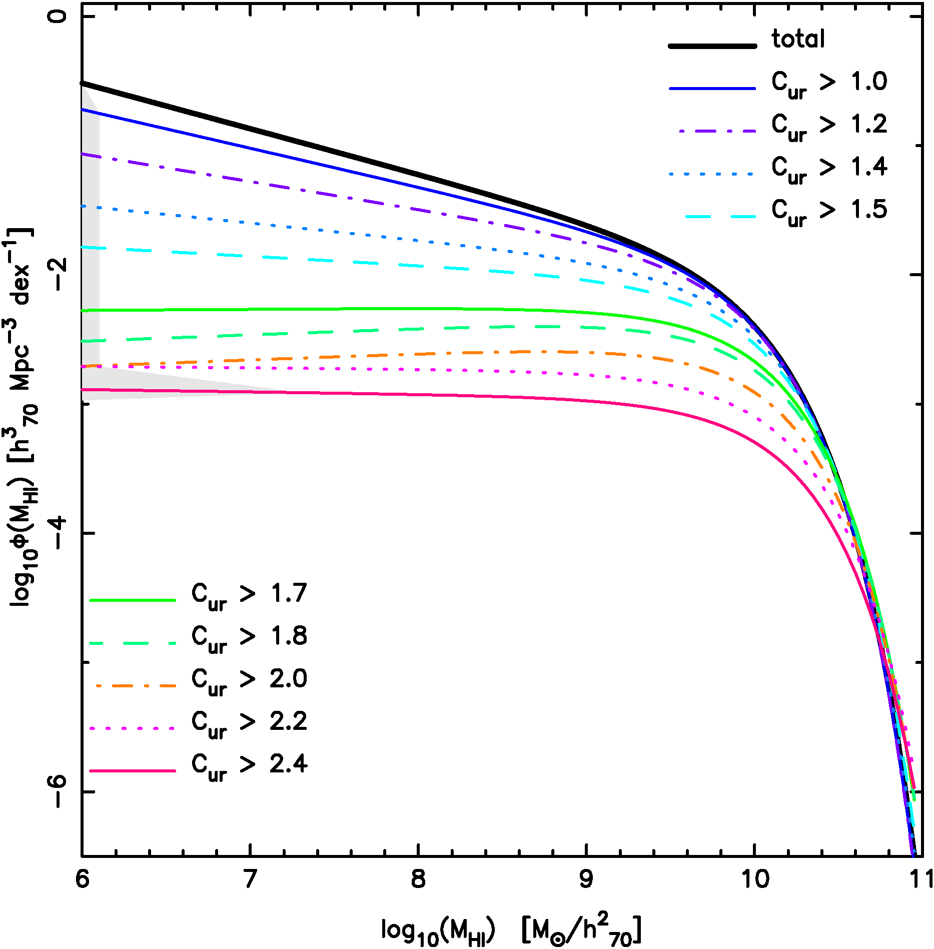
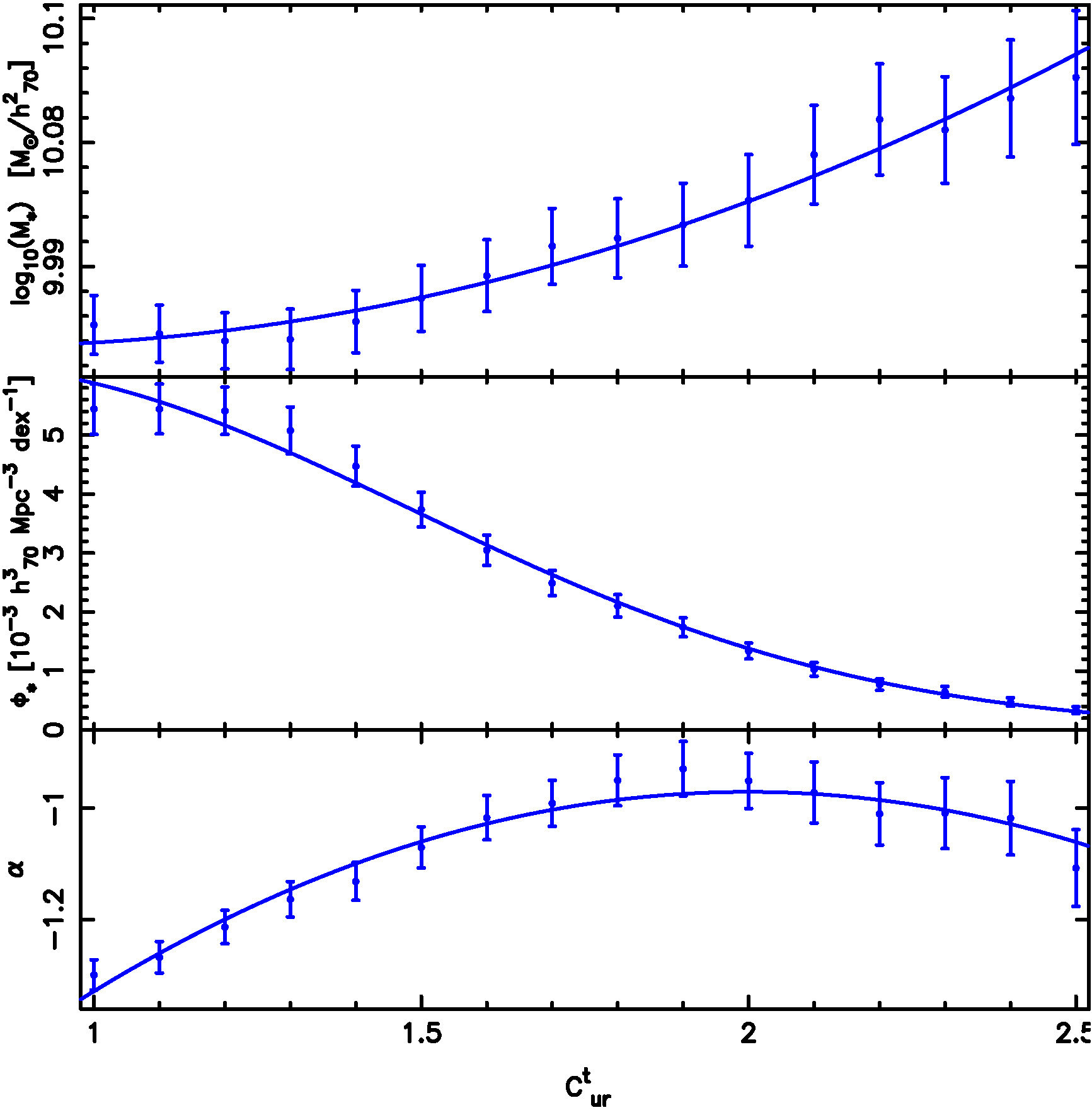
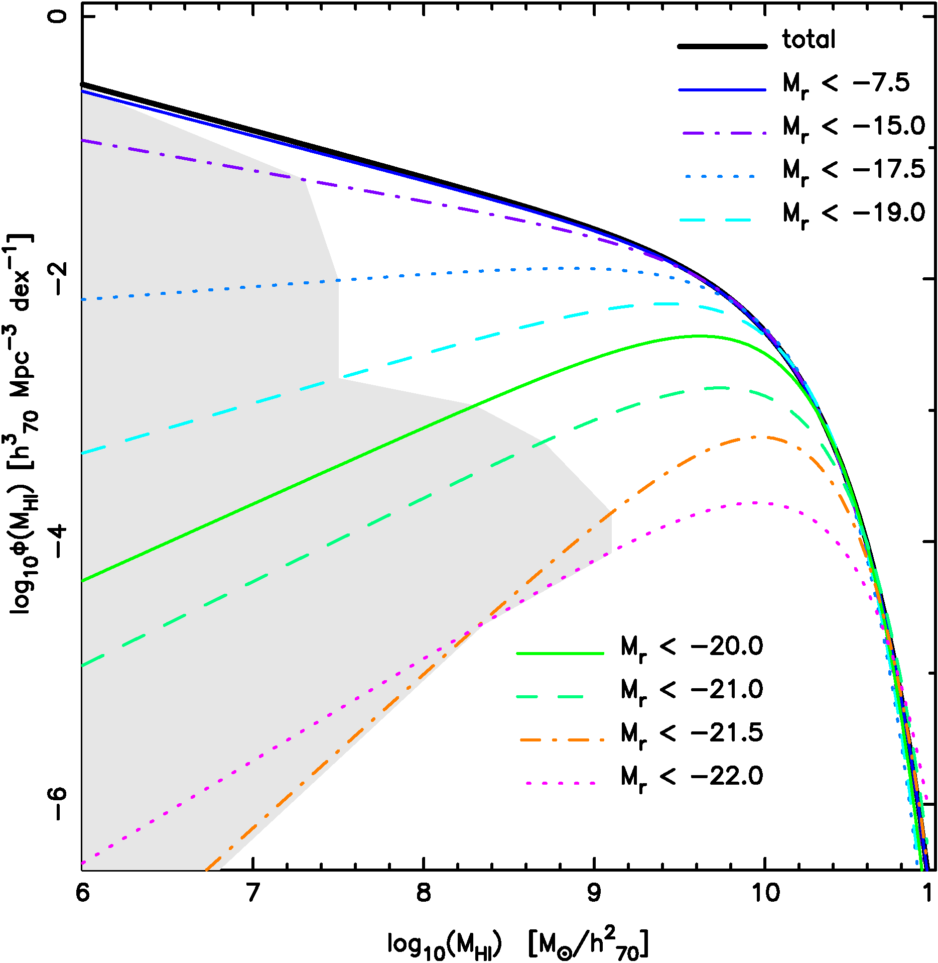
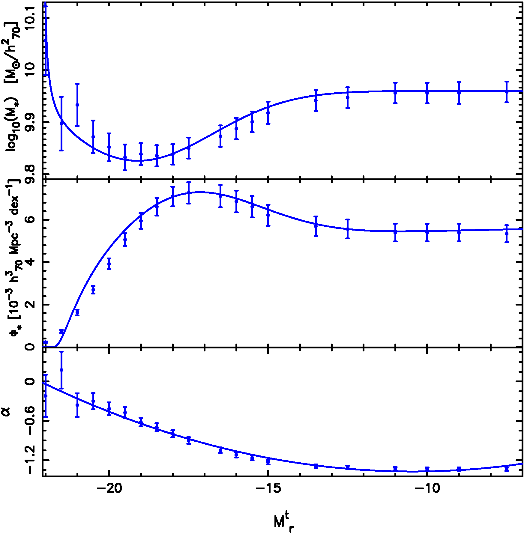
which represents the HIMF for galaxies which are more luminous than a threshold value $M_{\text{r}}^{t}$. To compute the conditional HIMF we start with the full sample of 7709 galaxies and create a subsample based on a threshold color $C_{\text{ur}}^{t}$ (or magnitude threshold $M_{\text{r}}^{t}$). We compute the HIMF for this subsample and also estimate its errors as outlined in section 3. We then fit a Schechter function to obtain a conditional HIMF for the particular subsample. We repeat this exercise to obtain the conditional HIMF as a function of $C_{\text{ur}}^{t}$ and $M_{\text{r}}^{t}$. Our results are shown in figures 1 and 2.

For the rest of the paper the values of the characteristic mass $M_{*}$ and the amplitude of the Schechter function $\phi_{*}$ (in equation 2) will be in the units $\left[\log(M_{*}/M_{\odot})+2\log h_{70}\right]$ and $\left[10^{-3}h_{70}^{3}Mpc^{-3}dex^{-1}\right]$ respectively. We will also quote $M_{\text{HI}}$ in the same units as $M_{*}$.

In the left panel of figures 1 and 2 we show the Schechter function fits to the conditional HIMF. The thick solid line is the HIMF for the full sample. The shaded gray patch represents the region where there is no data. While displaying the Schechter functions we have however extrapolated them to this region as well. The right panels represent the Schechter function fits and their uncertainties. The lines represent a parametric fit to these values. We note that the errorbars on the Schechter function parameters, although representative of the sample, are correlated, since the sample at each threshold (i.e. $C_{\text{ur}}^{t}$ or $M_{\text{r}}^{t}$) contains the sample of the previous neighboring threshold.

In figure 1 we look at the color-conditioned HIMF and its dependence on the threshold color $C_{\text{ur}}^{t}$. For $2.0\leq C_{\text{ur}}^{t}\leq 2.4$ the slope at the low mass end is flat, or $\alpha\sim-1$ (see bottom right panel of figure 1). At this end the amplitude, $\phi_{*}$ is small ($16\times$ smaller) compared to the amplitude of the total HIMF, $\phi_{*}=5.3\times 10^{-3}$, but the characteristic mass $M_{*}=10.13$ is about 50% larger than that of the HIMF of the full sample. A large value of $C_{\text{ur}}^{t}$ means that the subsample contains mostly redder galaxies. By decreasing this value we add blue galaxies to the sample and the conditional HIMF then approaches the total HIMF in the limit $C_{\text{ur}}^{t}\Rightarrow-\infty$. In our sample this is achieved when $C_{\text{ur}}^{t}=0$. As can be seen in figure 1 there is a near monotonic change in the shape (with the exception of $\alpha$) of the conditional HIMF with $C_{\text{ur}}^{t}$. Although $\alpha$ as a function of $C_{\text{ur}}^{t}$ peaks at about $C_{\text{ur}}^{t}=1.9$, the variation is still consistent with a constant value beyond that. Incidentally the peak in $\alpha$ occurs close to the value of the optimal divider of Baldry, et al. (2004) at $C_{\text{ur}}=2.3$ (see figure 3). The red population dominates the HIMF at the large mass end whereas decreasing the $C_{\text{ur}}^{t}$ we progressively add bluer galaxies to our sample which start to dominate the knee and then the low mass end for even smaller values of $C_{\text{ur}}^{t}$.

Figure 2: Left: Conditional HIMF as a function of decreasing rest frame magnitude thresholds (top to bottom). The thick solid line is the HIMF for the full sample. The shaded gray region does not contain data, the conditional HIMF have however been extrapolated into this regime as well. Right: The Schechter function parameters of the conditional HIMF and their uncertainties as a function of magnitude thresholds $M_{\text{r}}^{t}$. The solid lines are fits to the data points. For $\alpha$ (bottom) we fit with a quadratic function. For $M_{*}$ (top) and $\phi_{*}$ (middle) we fit with a function of the form: $y(x)=\left[a+b\exp\left(-\frac{(x+c)^{2}}{2d}\right)\right]\frac{f}{(x+e)}$.

In figure 2 we look at the dependence of the conditional HIMF on $M_{\text{r}}^{t}$. Unlike the previous case, the dependence of the conditional HIMF on $M_{\text{r}}^{t}$ is not monotonic (see right panel of figure 2). We see a dip (bump) in $M_{*}$ ($\phi_{*}$) at $M_{\text{r}}^{t}=19$ ($M_{\text{r}}^{t}\sim 17.5$). Coincidentally the distribution of the blue (red) population of galaxies is centered at $M_{\text{r}}=19$ ($M_{\text{r}}=20$) (See figure 3 of D20). As we move from the luminous ($M_{\text{r}}^{t}\leq 20$ dominated by the red sample), to the faint end, the conditional HIMF picks the contribution from the blue cloud at $M_{\text{r}}=19$. The bimodality of the underlying optical galaxy sample is reflected more strongly in the luminosity-conditioned HIMF than the color-conditioned HIMF.

4.2 The Distribution of $\Omega_{HI}$ in the $C_{\text{ur}}-M_{\text{r}}$ plane

We extend our previous definition to the two-dimensional conditional HIMF:

$$\phi(M_{\text{HI}}|C_{\text{ur}}^{t},M_{\text{r}}^{t})=\phi(M_{HI})|_{(C_{\text{ur}}>C_{\text{ur}}^{t}),(M_{\text{r}}<M_{\text{r}}^{t})}$$ (5)

This represents the HIMF of galaxies redder than $C_{\text{ur}}^{t}$ and more luminous than $M_{\text{r}}^{t}$, for which the corresponding HI density parameter is:

$$\Omega_{\text{HI}}(C_{\text{ur}}^{t},M_{\text{r}}^{t})=\frac{1}{\rho_{c}}\int_{0}^{\infty}M_{\text{HI}}\phi(M_{\text{HI}}|C_{\text{ur}}^{t},M_{\text{r}}^{t})dM_{\text{HI}}$$ (6)

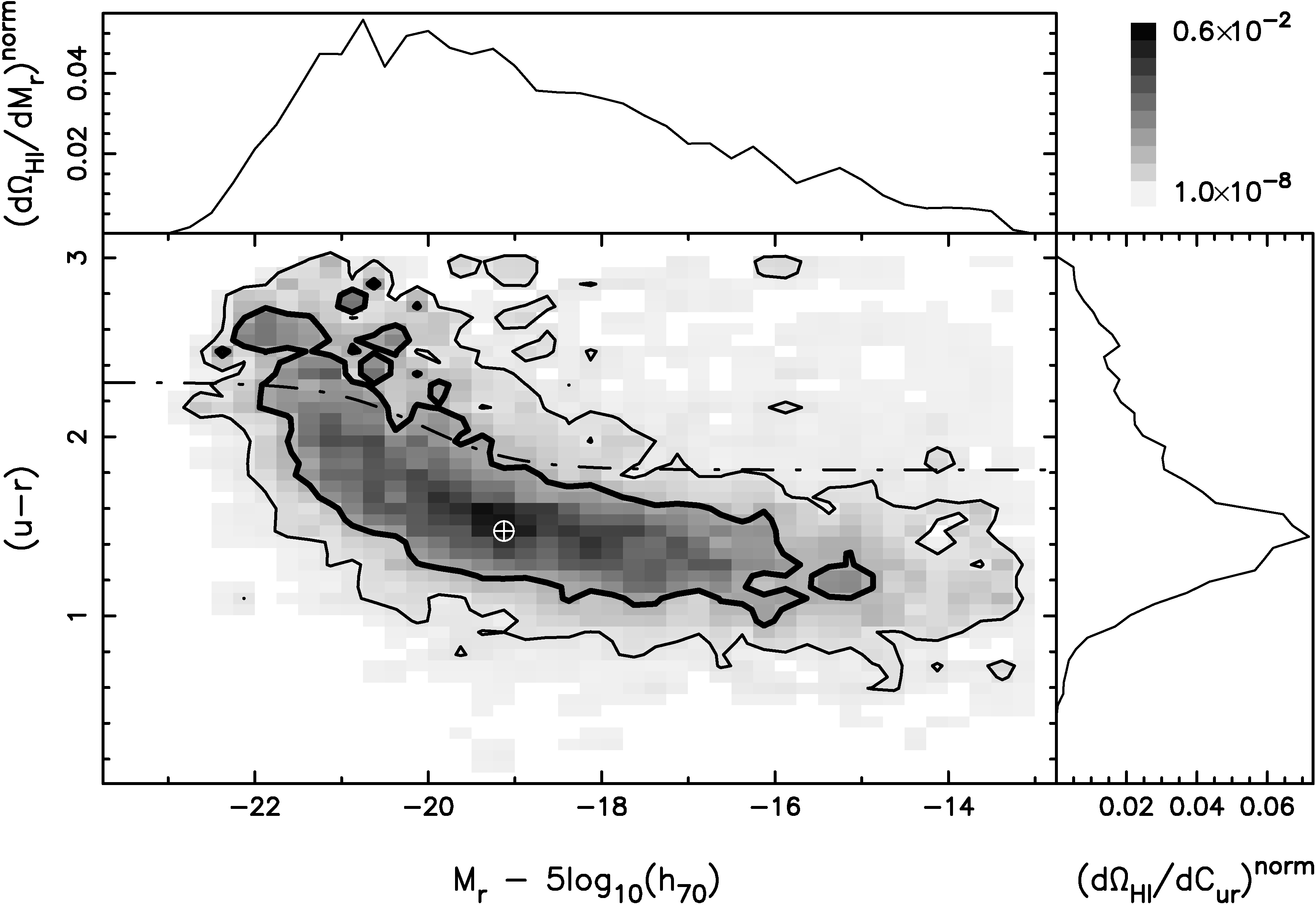
In our sample $\Omega_{\text{HI}}(C_{\text{ur}}^{t},M_{\text{r}}^{t})=\Omega_{\text{HI}}^{\text{tot}}=4.894\times 10^{-4}$ when $C_{\text{ur}}^{t}=0.0,M_{\text{r}}^{t}=-6.0$. We compute $2500$ conditional HIMFs and their associated errors in the CM plane by dividing $C_{\text{ur}}^{t}\in[3.0,0.0]$ (decreasing color threshold) and $M_{\text{r}}^{t}\in[-23.0,-6.0]$ (increasing magnitude threshold) into 50 bins each. From equation 6 we see that the variation of $\Omega_{\text{HI}}(C_{\text{ur}}^{t},M_{\text{r}}^{t})$ is that of a cumulant in the two-dimensional CM plane. If we define the normalized conditional HI density parameter as $\Omega_{\text{HI}}^{\text{norm}}(C_{\text{ur}}^{t},M_{\text{r}}^{t})=\frac{\Omega_{\text{HI}}(C_{\text{ur}}^{t},M_{\text{r}}^{t})}{\Omega_{\text{HI}}^{\text{tot}}}$, then $\Omega_{\text{HI}}^{\text{norm}}(C_{\text{ur}}^{t},M_{\text{r}}^{t})$ is bounded and varies from 0 (luminous-red, top left corner of figure 3) and 1 (faint-blue, bottom right corner of figure 3).

We define the distribution function of the cosmological HI density parameter in the CM plane

$$p\left(\Omega_{\text{HI}}(C_{\text{ur}},M_{\text{r}})\right)=\left.\frac{\partial^{2}\Omega_{\text{HI}}^{\text{norm}}(C_{\text{ur}}^{t},M_{\text{r}}^{t})}{\partial C_{\text{ur}}^{t}\partial M_{\text{r}}^{t}}\right|_{[C_{\text{ur}}^{t}=C_{\text{ur}},M_{\text{r}}^{t}=M_{\text{r}}]}$$ (7)

By construction this is a normalized distribution

$$\int\int p\left(\Omega_{\text{HI}}(C_{\text{ur}},M_{\text{r}})\right)\text{d}C_{\text{ur}}\text{d}M_{\text{r}}=1.0$$ (8)

The cosmological HI density in a given CM (ji) pixel is

$$(\Omega_{\text{HI}}^{ij})^{\text{norm}}=\int_{M_{\text{r}}^{i}}^{M_{\text{r}}^{i+1}}\int_{C_{\text{ur}}^{j}}^{C_{\text{ur}}^{j+1}}p\left(\Omega_{\text{HI}}(C_{\text{ur}},M_{\text{r}})\right)\text{d}C_{\text{ur}}\text{d}M_{\text{r}}$$ (9)

In figure 3 we plot the distribution function, $p(\Omega_{\text{HI}})$, of the cosmological HI density parameter in the CM plane. Each pixel is color-coded to the $(\Omega_{\text{HI}}^{ij})^{\text{norm}}$ value. The top left (bottom right) panel shows the marginalized distribution of $\Omega_{\text{HI}}$ as a function of magnitude (color). The dot-dashed line is the optimal divider which classifies these galaxies into red and blue populations (Baldry, et al., 2004). The thick (thin) contour is the $1\sigma$ ($2\sigma$) width of the distribution function, $p(\Omega_{\text{HI}})$ (i.e. the contour is determined from eq. 8 by setting the RHS to 0.68 (0.95)). The crossed-circle is the peak of $p(\Omega_{\text{HI}})$ in two dimensions, and does not match the peak of the marginalized distribution because it is skewed.

5 Discussion

In this paper we have presented the conditional HIMF, conditioned on color and/or magnitude. Based on the conditional HIMF we obtained the distribution of $\Omega_{\text{HI}}$, $p(\Omega_{\text{HI}})$, in the CM plane of galaxies. Not surprisingly our results for $\phi(M_{HI})|_{M_{\text{r}}<-21}$ and even brighter thresholds is similar to those obtained for the conditional HIMF, $\phi(M_{HI})|_{M_{\text{star}}\geq 10}$, for massive galaxies (Lemonias et al., 2013) from the GASS survey (Catinella, et al., 2010; Catinella et al., 2012); this is because the stellar mass of galaxies is correlated with its luminosity.

Both the two-dimensional and marginalized distributions show that they have long tail towards faint blue galaxies and luminous red galaxies. The peak of $p(\Omega_{\text{HI}})$ in the CM plane occurs at $C_{\text{ur}}^{\text{max}}=1.44,M_{\text{r}}^{\text{max}}=-19.25$ in the blue cloud, which is about 1.36 mag fainter than the characteristic luminosity of blue galaxies in SDSS (Baldry, et al., 2004). The width of $p(\Omega_{\text{HI}})$ is also fairly broad in both color and magnitude; the average $1\sigma$ ($2\sigma$) widths being $\sigma_{C}=0.8,\sigma_{M}=3.0$ ($\sigma_{C}=1.1,\sigma_{M}=4.8$). At the fainter end $M_{\text{r}}>-16$, $\sim 10\%$ of $\Omega_{\text{HI}}^{\text{tot}}$ is locked in gas rich low surface brightness galaxies. The red population, on the other hand, contributes $\sim 18\%$ to the HI budget.

The CM plane can be thought of as a coordinate system in which we can plot distributions of other cosmological density parameters (related to galaxies), $p(\Omega_{\text{X}})$ where X denotes a property, e.g. stellar mass $M_{\text{star}}$, $SFR$, molecular hydrogen mass $M_{\text{H}_{2}}$, which in turn are computed from $\phi(X|C_{\text{ur}}^{t},M_{\text{r}}^{t})$. We therefore have all the information needed to obtain the mean relation between different galaxy properties by discarding the common coordinate system. We emphasize that this relation is unbiased and represents the underlying relation since the distributions have folded in the survey selection. The blind nature of the survey is also important since there is no selection bias in estimating $\phi(X)$. This can be repeated for different galaxies populations (blue or red) and for other bands as well. The methods outlined in this paper are statistical in nature and provide a powerful and unbiased way to probe the multivariate distributions of galaxy populations. We will report on the mean HI-stellar mass relation in a forthcoming paper.

Figure 3: The bottom left panel shows the distribution function $p(\Omega_{HI})$ (see eq. 7) in the CM plane color coded by $(\Omega_{\text{HI}}^{ij})^{\text{norm}}$ (eq. 9). The thick (thin) line represent the $1\sigma$ ($2\sigma$) widths of $p(\Omega_{HI})$. The dash-dot line separates the optical red (above) and blue (below) populations (Baldry, et al., 2004). The top left (bottom right) panel is the marginalized distribution of $\Omega_{HI}$ as a function of $M_{r}$ ($C_{\text{ur}}$ ). The crossed circle represents the peak of the two-dimensional distribution function, $p(\Omega_{HI})$.

Data Availability

The data used in this work is publicly available. SDSS DR7 (Abazajian, et al., 2009) data can be accessed from sciserver.org and the $\alpha.40$ (Haynes, et al., 2011) data from ALFALFA can be accessed from egg.astro.cornell.edu.

References

- Abazajian, et al. (2009) Abazajian, K. N., et al. 2009,ApJS,182, 543
- Baldry, et al. (2004) Baldry, I. K., et al. 2004, ApJ,600,681
- Blanton & Roweis (2007) Blanton M. R., Roweis S., 2007, AJ, 133, 734
- Catinella, et al. (2010) Catinella B., et al., 2010, MNRAS, 403, 683
- Catinella et al. (2012) Catinella B., et al., 2012, A&A, 544, A65
- Dutta, Khandai, & Dey (2020) Dutta S., Khandai N., Dey B., (D20) 2020, MNRAS, 494, 2664
- Haynes, et al. (2011) Haynes M. P., et al., 2011, AJ, 142, 170
- Haynes, et al. (2018) Haynes M. P., et al., 2018 ApJ 861, 49
- Jones, et al. (2018) Jones, M.G., Haynes, M.P., Giovanelli, R. & Moorman, C. 2018 MNRAS 477, 2
- Kennicutt (1989) Kennicutt R. C., 1989, ApJ, 344, 685
- Kennicutt (1998) Kennicutt R. C., 1998, ApJ, 498, 541
- Lemonias et al. (2013) Lemonias J. J., Schiminovich D., Catinella B., Heckman T. M., Moran S. M., 2013, ApJ, 776, 74
- Loveday (2000) Loveday, J., 2000, MNRAS,312,557
- Martin, et al. (2010) Martin, A., et al., 2010, ApJ, 723,1359
- Morganti, et al. (2006) Morganti R., et al., 2006, MNRAS, 371, 157
- Oosterloo, et al. (2007) Oosterloo T. A., Morganti R., Sadler E. M., van der Hulst T., Serra P., 2007, A&A, 465, 787
- Schmidt (1959) Schmidt M., 1959, ApJ, 129, 243
- Schmidt (1963) Schmidt M., 1963, ApJ, 137, 758
- Serra, et al. (2012) Serra P., et al., 2012, MNRAS, 422, 1835
- Zwaan, Briggs, & Sprayberry (2001) Zwaan M. A., Briggs F. H., Sprayberry D., 2001, MNRAS, 327, 1249
- Zwaan, et al. (2003) Zwaan M. A., et al., 2003, AJ, 125, 2842