Price response functions and spread impact in correlated financial markets
Abstract
Recent research on the response of stock prices to trading activity revealed long lasting effects, even across stocks of different companies. These results imply non-Markovian effects in price formation and when trading many stocks at the same time, in particular trading costs and price correlations. How the price response is measured depends on data set and research focus. However, it is important to clarify, how the details of the price response definition modify the results. Here, we evaluate different price response implementations for the Trades and Quotes (TAQ) data set from the NASDAQ stock market and find that the results are qualitatively the same for two different definitions of time scale, but the response can vary by up to a factor of two. Further, we show the key importance of the order between trade signs and returns, displaying the changes in the signal strength. Moreover, we confirm the dominating contribution of immediate price response directly after a trade, as we find that delayed responses are suppressed. Finally, we test the impact of the spread in the price response, detecting that large spreads have stronger impact.
pacs:
89.65.GhEconophysics and 89.75.-kComplex systems and 05.10.GgStatistical physics1 Introduction
Financial markets use order books to list the number of shares bid or asked at each price. An order book is an electronic list of buy and sell orders for a specific security or financial instrument organized by price levels, where agents can place different types of instructions (orders).
In general, the dynamics of the prices follow a random walk. There are two extreme models that can describe this behavior: the Efficient Market Hypothesis (EMH) and the Zero Intelligence Trading (ZIT). The EMH states that all available information is included in the price and price changes can only be the result of unanticipated news, which by definition are totally unpredictable subtle_nature ; Bouchaud_2004 ; EMH_lillo ; stat_theory . On the other hand, the ZIT assumes that agents instead of being fully rational, have “zero intelligence” and randomly buy or sell. It is supposed that their actions are interpreted by other agents as potentially containing some information subtle_nature ; Bouchaud_2004 ; stat_theory ; Wang_2016_cross . In both cases the outcome is the same, the prices follow a random walk. Reality is somewhere in-between Bouchaud_2004 ; stat_theory , and non-Markovian effects due to stategies or liquidity costs are not contained either.
There are diverse studies focused on the price response prop_order_book ; dissecting_cross ; r_walks_liquidity ; subtle_nature ; Bouchaud_2004 ; large_prices_changes ; pow_law_dist ; theory_market_impact ; spread_changes_affect ; master_curve ; EMH_lillo ; quant_stock_price_response ; ori_pow_law ; Wang_2018_b ; Wang_2018_a ; Wang_2016_avg ; Wang_2016_cross . In our opinion, a critical investigation of definitions and methods and how they affect the results is called for.
Regarding price self-response functions in Refs. r_walks_liquidity ; subtle_nature ; Bouchaud_2004 , Bouchaud et al. found an increase to a maximum followed by a decrease as the time lag grows. In Ref. theory_market_impact , Gerig found that larger sized transactions have a larger absolute impact than smaller sized transactions but a much smaller relative impact. In Ref. prop_order_book , it is found that the impact of small trades on the price is, in relative terms, much larger than that of large trades and the impact of trading on the price is quasi-permanent.
For price cross-responses functions, Refs. dissecting_cross ; Wang_2016_cross revealed that the diagonal terms are on average larger than the off-diagonal ones by a factor . The response at positive times is roughly constant, what is consistent with the hypothesis of a statistically efficient price. Thus, the current sign does not predict future returns. In Ref. Wang_2016_cross the trends in the cross-responses were found not to depend on whether or not the stock pairs are in the same economic sector or extend over two sectors.
Here, we want to discuss, based on a series of detailed empirical results obtained on trade by trade data, that the variation in the details of the parameters used in the price response definition modify the characteristics of the results. Aspects like time scale, time shift, time lag and spread used in the price response calculation have an influence on the outcomes. To facilitate the reproduction of our results, the source code for the data analysis is available in Ref. code .
We delve into the key details needed to compute the price response functions, and explore their corresponding roles. We perform a empirical study in different time scales. We show that the order between the trade signs and the returns have a key importance in the price response signal. We split the time lag to understand the contribution of the immediate returns and the late returns. Finally, we shed light on the spread impact in the response functions for single stocks.
The paper is organized as follows: in Sect. 2 we present our data set of stocks. We then analyze the definition of the price response functions and describe the physical and trade time in Sect. 3. We implement different price responses for several stocks and pairs of stocks in Sect. 4. In Sect. 5 we show how the relative position between trade signs and returns has a huge influence in the results of the computation of the response functions. In Sect. 6 we explain in detail how the time lag behaves in the response functions. Finally, in Sect. 7 we analyze the spread impact in the price response functions. Our conclusions follow in Sect. 8.
2 Data set
Modern financial markets, are organized as a double continuous auctions. Agents can place different types of orders to buy or to sell a given number of shares, roughly categorized as market orders and limit orders.
In this study, we analyzed trades and quotes (TAQ) data from the NASDAQ stock market. We selected NASDAQ because it is an electronic exchange where stocks are traded through an automated network of computers instead of a trading floor, which makes trading more efficient, fast and accurate. Furthermore, NASDAQ is the second largest stock exchange based on market capitalization in the world.
In the TAQ data set, there are two data files for each stock. One gives the list of all successive quotes. Thus, we have the best bid price, best ask price, available volume and the time stamp accurate to the second. The other data file is the list of all successive trades, with the traded price, traded volume and time stamp accurate to the second. Despite the one second accuracy of the time stamps, in both files more than one quote or trade may be recorded in the same second.
To analyze the response functions across different stocks in Sects. 4, 5 and 6, we select the six companies with the largest average market capitalization (AMC) in three economic sectors of the S&P index in 2008. Table 1 shows the companies analyzed with their corresponding symbol and sector, and three average values for a year.
| Company | Symbol | Sector | Quotes1 | Trades2 | Spread3 |
|---|---|---|---|---|---|
| Alphabet Inc. | GOOG | Information Technology (IT) | |||
| Mastercard Inc. | MA | Information Technology (IT) | |||
| CME Group Inc. | CME | Financials (F) | |||
| Goldman Sachs Group Inc. | GS | Financials (F) | |||
| Transocean Ltd. | RIG | Energy (E) | |||
| Apache Corp. | APA | Energy (E) |
-
1
Average number of quotes from 9:40:00 to 15:50:00 New York time during 2008.
-
2
Average number of trades from 9:40:00 to 15:50:00 New York time during 2008.
-
3
Average spread from 9:40:00 to 15:50:00 New York time during 2008.
To analyze the spread impact in response functions (Sect. 7), we select 524 stocks in the NASDAQ stock market for the year 2008. The selected stocks are listed in Appendix A.
In order to avoid overnight effects and any artifact due to the opening and closing of the market, we systematically discard the first ten and the last ten minutes of trading in a given day Bouchaud_2004 ; large_prices_changes ; spread_changes_affect ; Wang_2016_cross . Therefore, we only consider trades of the same day from 9:40:00 to 15:50:00 New York local time. We will refer to this interval of time as the “market time”. The year 2008 corresponds to 253 business days.
3 Price response function definitions
In Sect. 3.1 we introduce the fundamental quantities used in the price response definitions. In Sect. 3.2 we describe the physical time scale and the trade time scale. We introduce the price response functions used in literature in Sect. 3.3.
3.1 Key concepts
Market orders are execute at the best available buy or sell price, limit orders set a maximum purchase price for a buy order, or a minimum sale price for a sell order. If the limit price is not matched, the order will not be carried out large_prices_changes ; predictive_pow ; intro_market_micro ; stat_theory . Limit orders often fail to result in an immediate transaction, and are stored in a queue called the limit order book prop_order_book ; stat_prop ; predictive_pow ; intro_market_micro . The order book also identifies the market participants behind the buy and sell orders, although some choose to remain anonymous. The order book is visible for all traders and its main purpose is to ensure that all traders have the same information on what is offered on the market. The order book is the ultimate microscopic level of description of financial markets.
Buy limit orders are called “bids”, and sell limit orders are called “asks”. At any given time there is a best (lowest) offer to sell with price , and a best (highest) bid to buy with price prop_order_book ; subtle_nature ; account_spread ; limit_ord_spread ; stat_theory . The price gap between them is called the spread subtle_nature ; market_digest ; Bouchaud_2004 ; account_spread ; large_prices_changes ; em_stylized_facts ; stat_theory . Spreads are significantly positively related to price and significantly negatively related to trading volume. Companies with more liquidity tend to have lower spreads components_spread_tokyo ; effects_spread ; account_spread ; components_spread .
The average of the best ask and the best bid is the midpoint price, which is defined as prop_order_book ; subtle_nature ; Bouchaud_2004 ; large_prices_changes ; em_stylized_facts ; stat_theory
| (1) |
As the midpoint price depends on the quotes, it changes if the quotes change. The midpoint price grows if the best ask or the best bid grow. On the other hand, the midpoint price decreases if the best ask or the best bid decrease.
Price changes are typically characterized as returns. If one denotes the price of an asset at time , the return , at time and time lag is simply the relative variation of the price from to subtle_nature ; empirical_facts ; asynchrony_effects_corr ; tick_size_impact ; causes_epps_effect ; non_stationarity ,
| (2) |
It is also common to define the returns as dissecting_cross ; subtle_nature ; empirical_facts ; empirical_properties ; large_prices_changes ; pow_law_dist ; theory_market_impact ; spread_changes_affect ; rand_mat ; fluctions_market_friction
| (3) |
Equations (2) and (3) agree if is small enough subtle_nature ; empirical_facts .
At longer timescales, midpoint prices and transaction prices rarely differ by more than half the spread. The midpoint price is more convenient to study because it avoids problems associated with the tendency of transaction prices to bounce back and forth between the best bid and ask large_prices_changes .
We define the returns via the midpoint price as
| (4) |
The distribution of returns is strongly non-Gaussian and its shape continuously depends on the return period . Small values have fat tails return distributions subtle_nature . The trade signs are defined for general cases as
| (5) |
where is a positive time increment. Hence we have
| (6) |
indicates that the trade was triggered by a market order to buy and a trade triggered by a market order to sell yields subtle_nature ; Bouchaud_2004 ; spread_changes_affect ; quant_stock_price_response ; order_flow_persistent .
It is well-known that the series of the trade signs on a given stock exhibit large autocorrelation. A very plausible explanation of this phenomenon relies on the execution strategies of some major brokers on given markets. These brokers have large transactions to execute on the account of some clients. In order to avoid market making movements because of an inconsiderable large order, they tend to split large orders into small ones empirical_facts .
3.2 Time definition
A direct comparison between the trade time scale and the physical time scale is not possible. To compare them directly we need to assume whether the midpoint price or the trade signs are on the same scale. We assume the midpoint prices in the trade time scale to be the same as the midpoint prices in physical time scale. Therefore, we have the time lag for both computations in seconds. This approximation allow us to directly compare both scales to have an idea of the difference and similarities they have. In the other sections, as we are not directly comparing the time scales, the corresponding quantities of each time scale are not mixed. Thus physical time scale is measured in seconds and trade time scale is measured in trades.
Due to the nature of the data, they are several options to define time for analyzing data.
In general, the time series are indexed in calendar time (hours, minutes, seconds, milliseconds). Moreover, tick-by-tick data available on financial markets all over the world is time stamped up to the millisecond, but the order of magnitude of the guaranteed precision is much larger, usually one second or a few hundreds of milliseconds market_digest ; empirical_facts . In several papers are used different time definitions (calendar time, physical time, event time, trade time, tick time) empirical_facts ; sampling_returns ; market_making . The TAQ data used in the analysis has the characteristic that the trades and quotes can not be directly related due to the time stamp resolution of only one second Wang_2016_cross . Hence, it is impossible to match each trade with the directly preceding quote. However, using a classification for the trade signs, we can compute trade signs in two scales: trade time scale and physical time scale.
The trade time scale is increased by one unit each time a transaction happens. The advantage of this count is that limit orders far away in the order book do not increase the time by one unit. The main outcome of trade time scale is its “smoothing” of data and the aggregational normality empirical_facts .
The physical time scale is increased by one unit each time a second passes. This means that computing the responses in this scale involves sampling sampling_returns ; Wang_2016_cross , which has to be done carefully when dealing for example with several stocks with different liquidity. This sampling is made in the trade signs and in the midpoint prices.
Facing the impossibility to relate midpoint prices and trade signs with the TAQ data in trade time scale, we will use the midpoint price of the previous second with all the trade signs of the current second. This will be our definition of trade time scale analysis for the response function analysis.
For physical time scale, as we can sampling, we relate the unique value of midpoint price of a previous second with the unique trade sign value of the current second.
Trade time scale
We use the trade sign classification in trade time scale proposed in Ref. Wang_2016_cross and used in Refs. Wang_2017 ; Wang_2018_copulas ; Wang_2016_avg that reads
| (7) |
implies a trade triggered by a market order to buy, and a value indicates a trade triggered by a market order to sell.
In the second case of Eq. (7), if two consecutive trades with the same trading direction did not exhaust all the available volume at the best quote, the trades would have the same price, and in consequence they will have the same trade sign.
With this classification we obtain trade signs for every single trade in the data set. According to Ref. Wang_2016_cross , the average accuracy of the classification is for the trade time scale.
The TAQ time step is one second, and as it is impossible to find the correspondences between trades and midpoint prices values inside a second step, We used the last midpoint price of every second as the representative value of each second. This introduce an apparent shift between trade signs and returns. In fact, we set the last midpoint price from the previous second as the first midpoint price of the current second Wang_2016_cross .
As we know the second in which the trades were made, we can relate the trade signs and the midpoint prices as shown in Fig. 1. For the trade time scale, there are in general, several midpoint prices in a second. For each second we select the last midpoint price value, and we relate it to the next second trades. In Fig. 1, the last midpoint price (circle) between the second and is related to all the trades (squares and triangles) in the second to , and so on. In the seconds when the quotes do not change, the value of the previous second (vertical line over the physical time interval) is used. Thus, all the seconds in the open market time have a midpoint price value, and in consequence returns values. We assume that as long as no changes occurred in the quotes, the midpoint price remains the same as in the previous second.

The methodology described is an approximation to compute the response in the trade time scale. A drawback in the computation could come from the fact that the return of a given second is composed by the contribution of small returns corresponding to each change in the midpoint price during a second. As we are assuming only one value for the returns in each second, we consider all the returns in one second interval to be positive or negative with the same magnitude, which could not be the case. This could increase or decrease the response signal at the end of the computation.
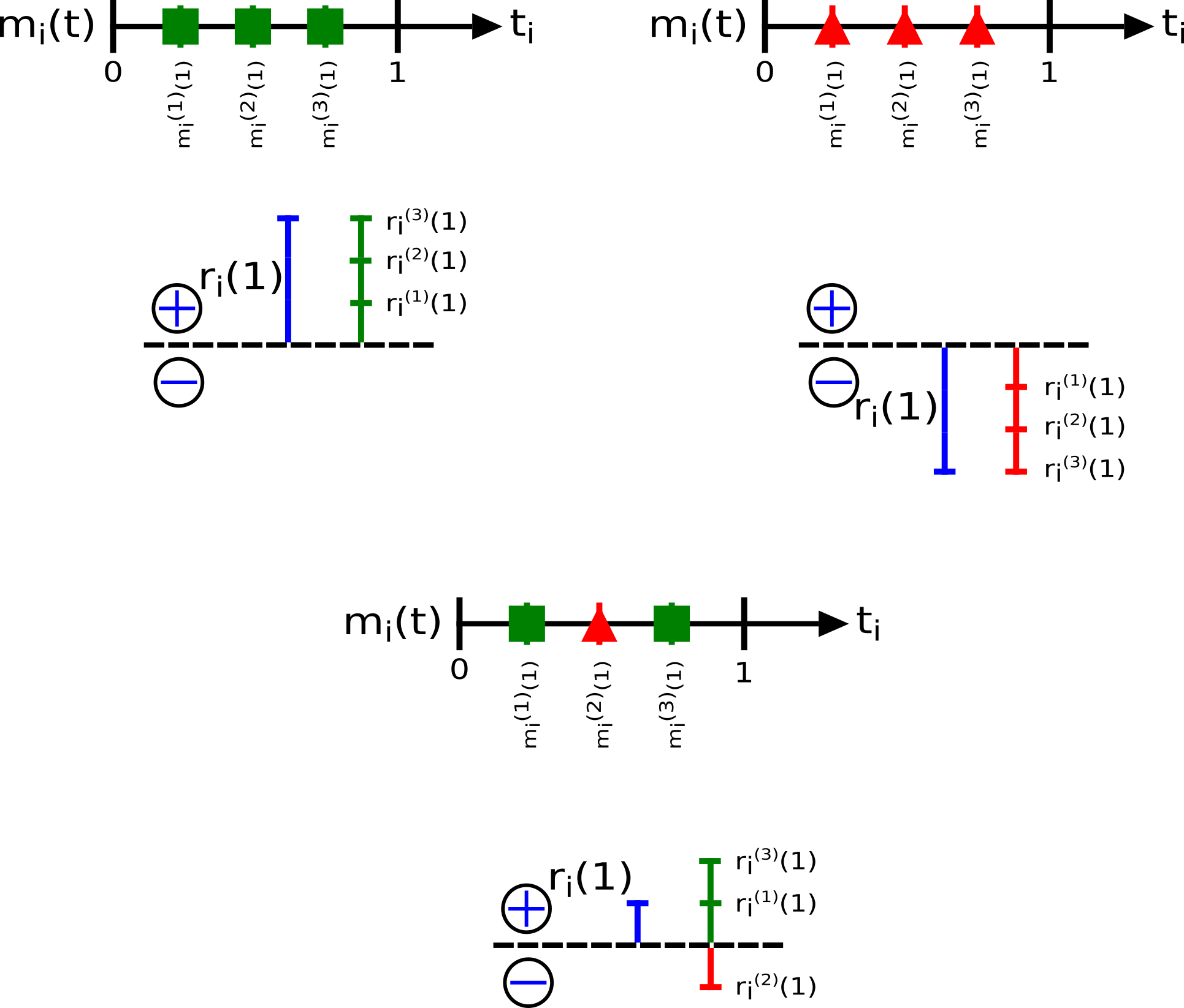
Figure 2 illustrate this point. Suppose there are three different midpoint prices in one second interval and thus, three different returns for these three midpoint price values. Furthermore, suppose that the volume of limit orders with the corresponding midpoint prices are the same in the bid and in the ask (the returns have the same magnitude). In the case of the top left (top right) sketch, all the changes are due to the rise (decrease) of the midpoint price, that means, consumption of the best ask (bid), so all the contributions of the individual returns in the second are positive (negative), and in consequence, the net return is positive (negative). In the case of the bottom, the changes are due to a combination of increase and decrease of the midpoint price, so in the end, the individual returns sum up to a net return, which can be positive or negative, depending of the type of midpoint price values in the interval. Thus, in this case, we are assuming in the end that all the returns were positive or negative, which probably was not the case, and in consequence will increase or decrease the real value of the net return.
In all cases, we choose the last change in the midpoint price in a second interval as described before in Fig. 1. We use this method knowing that the variation in one second of the midpoint price is not large (in average, the last midpoint price of a second differ with the average midpoint of that second in ), hence it can give us representative information on the response functions.
Physical time scale
We use the trade sign definition in physical time scale proposed in Ref. Wang_2016_cross and used in Refs. Wang_2017 ; Wang_2016_avg , that depends on the classification in Eq. (7) and reads
| (8) |
where is the number of trades in a second interval. implies that the majority of trades in second were triggered by a market order to buy, and a value indicates a majority of sell market orders. In this definition, they are two ways to obtain . One way is that in a particular second there are no trades, and then no trade sign. The other way is that the addition of the trade signs ( and ) in a second be equal to zero. In this case, there is a balance of buy and sell market orders.
Market orders show opposite trade directions to limit order executed simultaneously. An executed sell limit order corresponds to a buyer-initiated market order. An executed buy limit order corresponds to a seller-initiated market order.
As the trade time scale, on the physical time scale we use the same strategy to obtain the midpoint price for every second, so all the seconds in the open market time have a midpoint price value. Even if there is no change of quotes in a second, it still has a midpoint price value and return value.

In this case we do not compare every single trade sign in a second, but the net trade sign obtained for every second with the definition, see Eq. (8). This can be seen in Fig. 3, where we related the midpoint price of the previous second with the trade sign of the current second. According to Ref. Wang_2016_cross , this definition has an average accuracy up to in the physical time scale.
3.3 Response function definitions
The response function measures price changes resulting from execution of market orders. In Refs. r_walks_liquidity ; subtle_nature ; Bouchaud_2004 , Bouchaud et al. use a self-response function that only depends on the time lag . This function measures how much, on average, the price moves up (down) at time conditioned to a buy (sell) order at time zero. They found for France Telecom that the response function increases by a factor between and trades, before decreasing back. For larger , the response function decreases, and even becomes negative beyond . However, in some cases the maximum is not observed and rather the price response function keeps increasing mildly subtle_nature .
In Ref. theory_market_impact , the price impact function, is defined as the average price response due to a transaction as a function of the transaction’s volume. Empirically the function is highly concave theory_market_impact . The curvature of the price impact function is entirely due to the probability that a transaction causes a nonzero impact. The larger the size of the transaction, the larger the probability. In Ref. prop_order_book , they found that the response function for three French stocks first increases from to a few hundred seconds, and then appears to decrease back to a finite value.
In Ref. dissecting_cross they defined a response function who measures the average price change of a contract at time , after experiencing a sign imbalance in contract at time . In this work is used in units of five minutes.
In later works spread_changes_affect ; Wang_2016_cross , Grimm et al. and Wang et al. use the logarithmic return for stock and time lag , defined via the midpoint price to define a cross-response function. The response function measures how a buy or sell order at time influences on average the price at a later time . The physical time scale was chosen since the trades in different stocks are not synchronous (TAQ data). They found that in all cases, an increase to a maximum is followed by a decrease. The trend is eventually reversed.
Finally, in Ref. Wang_2018_b , Wang et al. define the response function on a trade time scale (Totalview data), as the interest is to analyze the immediate responses. Here, the time lag is restricted to one trade, such that the price response quantifies the price impact of a single trade.
4 Price response function implementations
The main objective of this work is to analyze the price response functions. In general we define the self- and cross-response functions in a correlated financial market as
| (9) |
where the index and correspond to stocks in the market, is the return of the stock in a time lag in the corresponding scale and is the trade sign of the stock in the corresponding scale. The superscript refers to the time scale used, whether physical time scale () or trade time scale (). Finally, The subscript refers to the way to average the price response, whether relative to the physical time scale () or relative to the trade time scale ().
We use the returns and the trade signs to define three response functions: trade time scale response, physical time scale response and activity response.
To compare the three response functions, we define the following quantities
| (10) | ||||
| (11) |
where the subscript refers to the days used in the response computation. We use Eq. (10) to make easier the comparison between the results, as all the defined responses use the trade sign term.
In Sect. 4.1 we analyze the responses functions in trade time scale, in Sect. 4.2 we analyze the responses functions in physical time scale and in Sect. 4.3 we define a response function to analyze the influence of the frequency of trades in a second.
4.1 Response functions on trade time scale
We define the self- and cross-response functions in trade time scale, using the trade signs in trade time scale. For the returns, we select the last midpoint price of every second and compute them. We use this strategy with the TAQ data set considering that the price response in trade time scale can not be directly compared with the price response in physical time scale. In this case we relate each trade sign in one second with the midpoint price of the previous second. Then, to compute the returns, instead of using trades as the time lag (it would make no sense as all the midpoint price are the same in one second) we use seconds. Thus, we force the response in trade time scale to have a physical time lag, and then, be able to compare with the physical time scale response. This approximation is feasible considering the discussion in Sect. 3. The price response function in trade time scale is defined as
| (12) |
where the superscript refers to the trade time scale. We explicitly calculate the average in Eq. (12),
| (13) | ||||
| (14) |
where
| (15) |
is a weight function that depends on the normalization of the response.
To compute the response functions on trade time scale, we used all the trade signs during a day in market time. As we can not associate an individual midpoint price with their corresponding trade signs, all the trade signs in one second are associated with the midpoint price of the previous second. As depends on the midpoint price, even if we are using trade signs in trade time scale, the value of is in seconds.
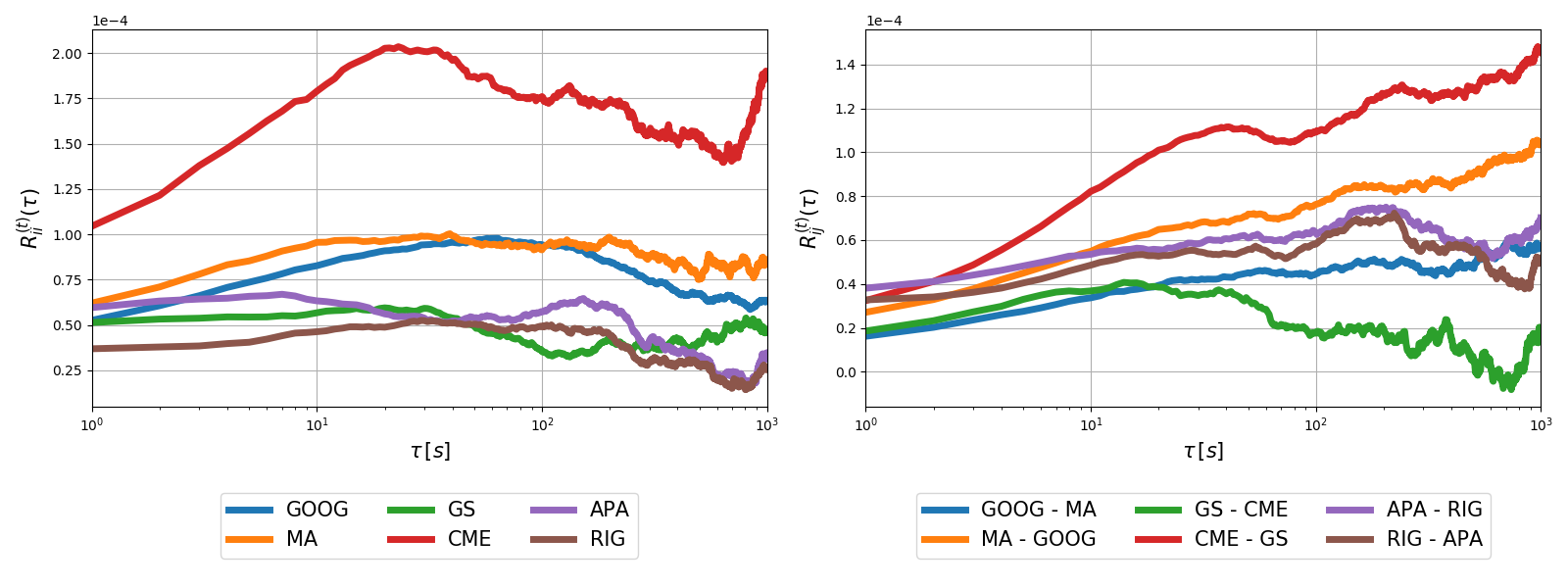
The results of Fig. 4 show the self- responses of the six stocks used in the analysis and the cross-responses for pairs of stocks representing three different economic sectors.
The self-response functions increase to a maximum and then slowly decrease. In some stocks this behavior is more pronounced than in others. For our selected tickers, a time lag of is enough to see an increase to a maximum followed by a decrease. Thus, the trend in the self-response functions is eventually reversed. On the other hand, the cross-response functions have smaller signal strength than the self-response functions. For our cross-response functions of stocks in the same sectors, some couples exhibit the increase-decrease behavior inside a time lag of . Other couples seems to need a larger time lag to reach the decrease behavior.
4.2 Response functions on physical time scale
One important detail to compute the market response in physical time scale is to define how the averaging of the function will be made, because the response functions highly differ when we include or exclude Wang_2016_cross . The price responses including are weaker than the excluding ones due to the omission of direct influence of the lack of trades. However, either including or excluding does not change the trend of price reversion versus the time lag, but it does affect the response function strength Wang_2016_avg . For a deeper analysis of the influence of the term , we suggest to check Refs. Wang_2016_avg ; Wang_2016_cross . We will only take in account the response functions excluding .
We define the self- and cross-response functions in physical time scale, using the trade signs and the returns in physical time scale. The price response function on physical time scale is defined as
| (16) |
where the superscript refers to the physical time scale. The explicit expression corresponding to Eq. (16) reads
| (17) | ||||
| (18) |
where
| (19) |
take only in account the seconds with trades and
| (20) |
is a weight function that depends on the normalization of the response.
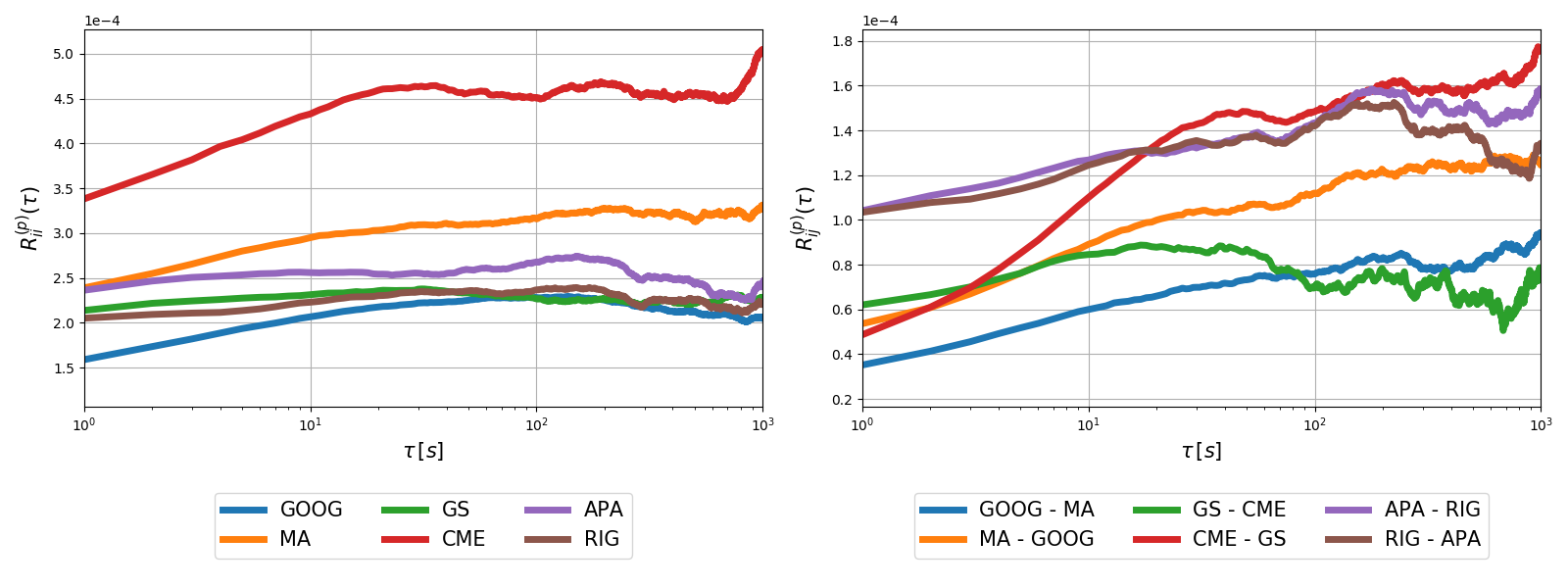
The results showed in Fig. 5 are the self- and cross-response functions in physical time scale. For the self-response functions we can say again that in almost all the cases, an increase to a maximum is followed by a decrease. Thus, the trend in the self- and cross-response is eventually reversed. In the cross-response functions, we have a similar behavior with the previous subsection, where the time lag in some pairs was not enough to see the decrease of the response.
Compared with the response functions in trade time scale, the response functions in physical time scale are stronger.
4.3 Activity response functions on physical time scale
Finally, we define the activity self- and cross-response functions in physical time scale, using the trade signs and the returns in physical time scale. We add a factor to check the influence of the frequency of trades in a second in the response functions. The activity price response function is defined as
| (21) |
where the superscript refers to the activity response function. The corresponding explicit expression reads
| (22) | ||||
| (23) |
where
| (24) |
is a weight function that depends on the normalization of the response.
As is the sum of and in one second and is the number of trades in a second, . only when all the trades in a second are buys .
The trade weight reduces noises, The physical weight gives every step the same weight, and the activity weight emphasizes seconds with large activity.
In Fig. 6, we can see how the three responses have approximately the same shape, but the strength of the signal varies depending on the definition. The frequency of trades have a large influence in the responses.
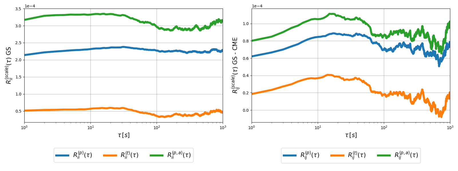
As predicted by the weights, the event response is weaker than the physical response, and the activity response is the strongest response.
We propose a methodology to directly compare price response functions in trade time scale and physical time scale. Additionally, we suggest a new definition to measure the impact of the number of trades in physical time scale. In the three curves in the figure can be seen the increase-decrease behavior of the response functions.
Our results are consistent with the current literature, where the results differ about a factor of two depending on the time scale. We note that the activity response function implementation is only a test and was never defined in previous works. That is why the difference of a factor of two can not be seen in Fig. 6 for .
5 Time shift response functions
The relative position between returns and trade signs directly impact the result of the response functions. Shifting the values to the right or to the left either in trade time scale or physical time scale have approximately the same effect.
To test this claim, we used the definition of the response function from Ref. Wang_2016_cross and add a parameter that shifts the position between returns and trade signs. To see the impact of the time shift we analyzed the stocks showed in Table 1 in the year 2008. We used different time shifts in the response function
| (25) |
where the index and correspond to stocks in the market, is the return of the stock in a time lag with a time shift in the corresponding scale and is the trade sign of the stock in the corresponding scale. The superscript refers to the time scale used, whether physical time scale () or trade time scale (). is the time shift price response function, where the superscript refers to the time shift. Finally, The subscript refers to the way to average the price response, whether relative to the physical time scale () or relative to the trade time scale ().
We compute the response functions according to two cases. In one case we set to a constant value and vary , and in the other case we set to a constant value and vary .
In Sect. 5.1 we analyze the influence of the time shift between the trade signs and returns in trade time scale and in Sect. 5.2 we analyze the influence of the time shift between the trade signs and returns in physical time scale.
5.1 Trade time scale shift response functions
On the trade time scale we compute the response function
| (26) |
In this case for , we associate all the trade signs to a return value and create pseudo midpoint price values in trade time scale. Then, we shift the trade signs and the returns by trades. Hence, the time lag and time shift are in trade time scale.
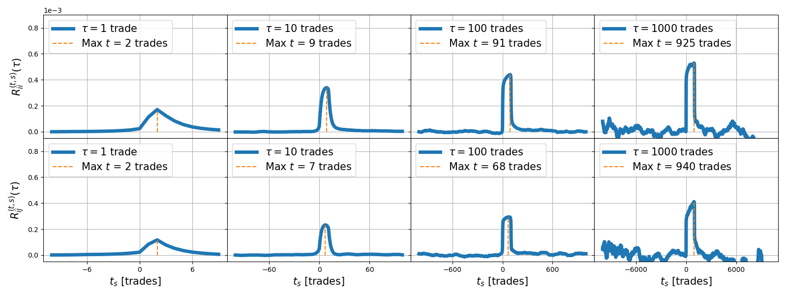
In Fig. 7, we show the response functions results for fixed values while is variable. In the different values figures, the results are almost the same. The response functions are zero either if the time shift is larger than , or if the time shift is smaller than zero. However, related to the time lag, there is a zone where the signal is different from zero. For values between zero and there is a peak in a position related to . The response function grows and decreases relatively fast.
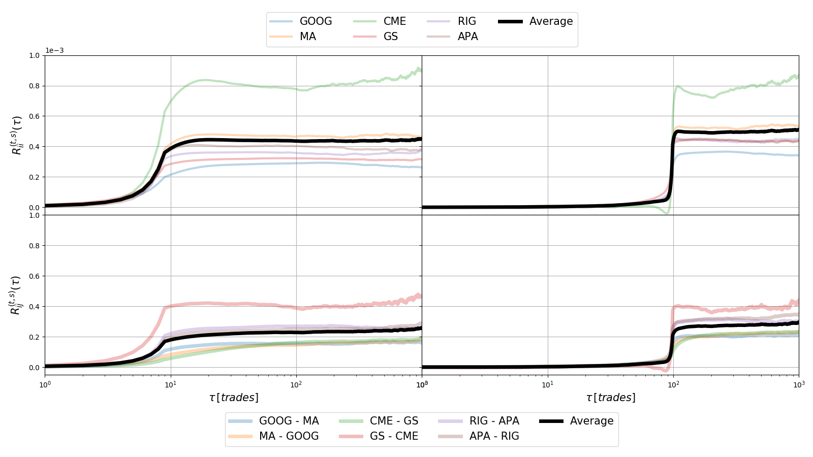
We tested the response function for fixed time shift values while is variable. In Fig. 8 we use a time shift of trades (left) and trades (right). In both, self- and cross-response results are qualitatively the same. It can be seen that the response functions have a zero signal before the time shift. After the returns and trade signs find their corresponding order the signals grow. In comparison with the values obtained in Fig. 4, it looks like the response function values with large time shift are stronger. However, this is an effect of the averaging of the functions. As the returns and trade signs are shifted, there are less values to average, and then the signals are stronger. Anyway, the figure shows the importance of the position order between the trade signs and returns to compute the response function.
5.2 Physical time scale shift response functions
In the physical time scale we compute the response function
| (27) |
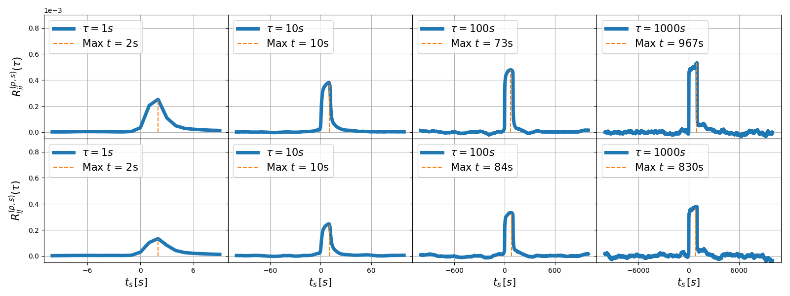
Similar to the results in Subsect. 5.1, Fig. 9 shows the responses functions for fixed values while is variable. Again, the response functions are zero if the time shift is larger than the time lag, or if the time shift is smaller than zero. For every value, there is a peak. The peak grows and decay relatively fast. The response signal usually starts to grow in zero or a little bit earlier and grows to a value around to . In this zone the response functions are different to zero.
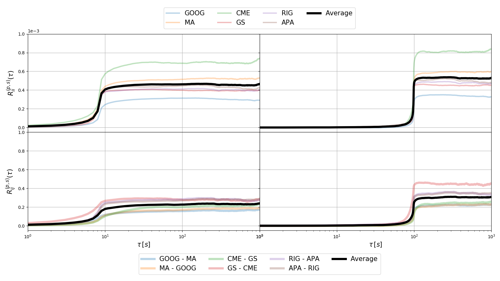
The results for fixed time shift values and variable time lag ( and ) are shown in Fig. 10. The self- and cross-response results are qualitatively the same compared with the previous subsection. The response functions are zero before the time shift value. After the returns and the trade signs reach their order, the signals grow. The same effect of the apparent stronger signal can be seen here, and again, it is due to the averaging values.
The results in trade time scale and physical time scale can be explained understanding the dynamics of the market. A trade can or can not change the price of a ticker. Therefore, when a change in price happens, a change in midpoint price, and consequently in returns happens. Thus, it is extremely important to keep the order of the events and the relation between them. When we shift the trade signs and returns, this order is temporarily lost and as outcome the signal does not have any meaningful information. When the order is recovered during the shift, the signal grows again, showing response function values different to zero. In this section we were interested only in the order (shift) and not in the responses values, which were analyzed in Sect. 4. A time shift smaller than zero does not have any useful information about the response. If the time shift is equal to zero, the signal is weak, due to the time needed by the market to react to the new information. On the other hand, a time shift larger than two steps shows the information is lost and the signal only grows when the original order is resumed.
Then the question is what is the ideal time shift to compute the response functions. Our approach in Sect. 4 takes in account that the changes in the quotes are the ones that attract the agents to buy or sell their shares. Hence, they directly impact the trade signs. According to the results, the response can take up to two time steps in the corresponding scale to react to the change in quotes. Thus, a time shift larger than two time steps makes no sense. On the other hand, in the case of the physical time scale, where a sampling is used, to assure the selection of a midpoint price at the beginning of a second, it is a good strategy to use the last midpoint of the previous second as the first midpoint price of the current second. In this case an apparent one second shift is used between returns and trade signs.
6 Time lag analysis
Regarding Equation (2), we use a time lag in the returns to see the gains or loses in a future time. However, the strength of the return in the time lag should not be equal along its length. Then, we divide the full range time lag in an immediate time lag and in a late time lag as show in Fig. 11, where

| (28) |
for . This distinguish the returns depending on the time lag as the short (immediate) return with the long return . This approach is similar to the concept used in Ref. Wang_2018_b , where the price impact for a single trade is estimated by the immediate response on an event time scale. In our case, we check all over the range of the time lag in the price response function on a physical time scale.
To use the short and long time lag, we rewrite the returns in physical time scale as
| (29) |
where the superscript refers to short-long and the second term of the right part is constant with respect to . Replacing Eq. (6) in the price response function in physical time scale (Eq. (16)) we have
| (30) |
Where the first term in the right side of Eq. (6) is the long response and the right term is the short response. Again, the right term of Eq. (6) is independent of .
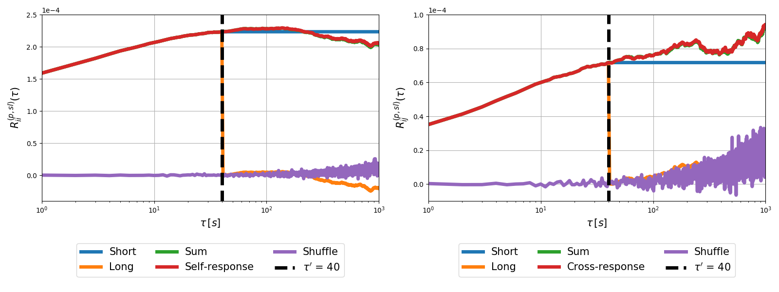
The results in Fig. 12 show the short response, the long response, the addition of the short response and long response (Sum), the original response, a random response and the value of .
The main signal of the response function come from the short response. Depending on the stock and the value of the long response can increase or decrease the short response signal, but in general the long response does not give a significant contribution to the complete response.
Before , the short response and long response are the same, as the self and cross-response definition do not define values smaller than , so it is computed as the original response. In the figure, the curves of the short and long response are under the curve of the original response. After , the short response is a strong constant signal. On the other hand, the long response immediately fades, showing the small contribution to the final response. To compare the significance of the long response, We added a random response made with the trade signs used to compute the response but with a shuffle order. The long response and the random response are comparable, and show how the long response is not that representative in the final response. If we add the short and long response, we obtain the original response. In Fig. 12, the original response (red line) has the same shape to the addition of the short and long response (green line).
For the response functions that show the increase-decrease behavior in between the time lag , the peak is usually between and . In these cases the long response are always negative after the value and is comparable in magnitude with the random signal. On the other hand, the response functions that requires a bigger time lag to show the increase-decrease behavior, have non negative long responses, but still they are comparable in magnitude with the random signal.
According to our results, price response functions show a large impact on the first instants of the time lag. We proposed a new methodology to measure this effect and evaluate their consequences. The short response dominates the signal, and the long response vanishes.
7 Spread impact in price response functions
When we calculate the price response functions, the signal of the response depends directly on the analyzed stock. Thus, even if the responses functions are in the same scale, their values differ from one to another. We choose the spread reg_and_irreg to group 524 stocks in the NASDAQ stock market for the year 2008 in physical time scale, and check how the average strength of the price self-response functions in physical time scale behaved for this groups. For each stock we compute the spread in every second along the market time. Then we average the spread during the 253 business days in 2008. With this value we group the stocks.
We used three intervals to select the stocks groups (, and ). The detailed information of stocks, the spread and the groups can be seen in Appendix A. With the groups of the stocks defined, we averaged the price response functions of each group.
In Fig. 13 we show the average response functions for the three groups. The average price response function for the stocks with smaller spreads (more liquid) have in average the weakest signal in the figure. On the other hand, the average price response function for the stocks with larger spreads (less liquid) have in average the strongest signal. According to the results described in Sect. 3 and 4, the average price response functions for all the groups follow the increment to a maximum followed by a decrease in the signal intensity.
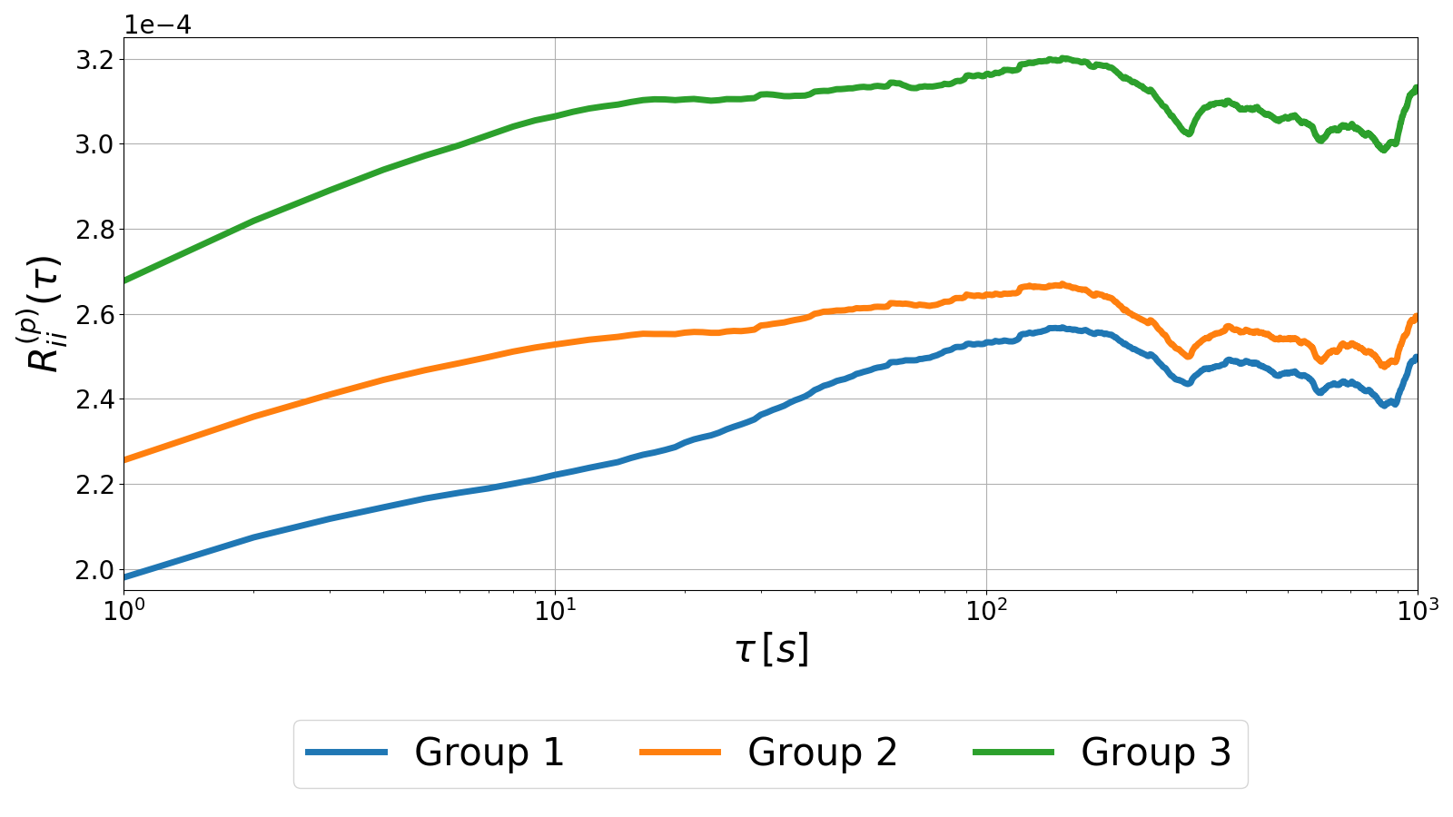
The strength of the price self-response function signals grouped by the spread can be explained knowing that the response functions directly depend on the trade signs. As long as the stock is liquid, the number of trade signs grow. Thus, at the moment of the averaging, the large amount of trades, reduces the response function signal. Therefore, the response function decrease as long as the liquidity grows, and as stated in the introduction the spread is negatively related to trading volume, hence, firms with more liquidity tend to have lower spreads.
Finally, an interesting behavior can be seen in Fig. 13. Despite each stock has a particular price response according to the returns and trade signs, the average price response function for the different groups seems to be quite similar. As all the analyzed stocks come from the same market we can infer that the general behavior of the market affect all the stocks, influencing in average a group response.
8 Conclusion
We went into detail about the response functions in correlated financial markets. We define the trade time scale and physical time scale to compute the self- and cross-response functions for six companies with the largest average market capitalization for three different economic sectors of the S&P index in 2008. Due to the characteristics of the data used, we had to classify and sampling values to obtain the corresponding quantities in different time scales. The classification and sampling of the data had impact on the results, making them smoother or stronger, but always keeping their shape and behavior.
The response functions were analyzed according to the time scales. We proposed a new approach to compare price response functions from different scales. We used the same midpoint prices in physical time scale with the corresponding trade signs in trade time scale or physical time scale. This assumption allowed us to compare both price response functions and get an idea of how representative was the behavior obtained in both cases. For trade time scale, the signal is weaker due to the large averaging values from all the trades in a year. In the physical time scale, the response functions had less noise and their signal were stronger. We proposed an activity response to measure how the number of trades in every second highly impact the responses. As the response functions can not grow indefinitely with the time lag, they increase to a peak, to then decrease. It can be seen that the market needs time to react and revert the growing. In both time scale cases depending on the stocks, two characteristics behavior were shown. In one, the time lag was large enough to show the complete increase-decrease behavior. In the other case, the time lag was not enough, so some stocks only showed the growing behavior.
We modify the response function to add a time shift parameter. With this parameter we wanted to analyze the importance in the order of the relation between returns and trade signs. In trade time scale and physical time scale we found similar results. When we shift the order between returns and trade signs, the information from the relation between them is temporarily lost and as outcome the signal does not have any meaningful information. When the order is recovered, the response function grows again, showing the expected shape. We showed that this is not an isolated conduct, and that all the shares used in our analysis exhibit the same behavior. Thus, even if they are values of time shift that can give a response function signal, empirically we propose this time shift should be a value between time steps.
We analyzed the impact of the time lag in the response functions. We divided the time lag in a short and long time lag. With this division we adapted the price response function in physical time scale. The response function that depended on the short time lag, showed a stronger response. The long response function vanish, and depending on the stock could take negative and non-negative values comparable to a random signal.
Finally, we checked the spread impact in price self-response functions. We divided 524 stocks from the NASDAQ stock market in three groups depending on the year average spread of every stock. The response functions signal were stronger for the group of stocks with the larger spreads and weaker for the group of stocks with the smaller spreads. A general average price response behavior was spotted for the three groups, suggesting a market effect on the stocks.
9 Author contribution statement
TG proposed the research. SMK and JCHL developed the method of analysis. The idea to look the time shift and to analyze the spread impact was due to JCHL, and the idea of the time lag analysis was due to SMK. JCHL carried out the analysis. All the authors contributed equally to analyze the results and write the paper.
Acknowledgements.
We thank S. Wang for fruitful discussions. One of us (JCHL) acknowledges financial support from the German Academic Exchange Service (DAAD) with the program “Research Grants - Doctoral Programmes in Germany” (Funding programme 57381412)Appendix A NASDAQ stocks used to analyze the spread impact
We analyzed the spread impact in the response functions for 524 stocks from the NASDAQ stock market for the year 2008. In Tables LABEL:tab:spread_comp_1, LABEL:tab:spread_comp_2, LABEL:tab:spread_comp_3 and LABEL:tab:spread_comp_4, we listed the stocks in their corresponding spread groups.
References
- [1] More statistical properties of order books and price impact. Physica A: Statistical Mechanics and its Applications, 324(1):133 – 140, 2003. Proceedings of the International Econophysics Conference.
- [2] Hee-Joon Ahn, Jun Cai, Yasushi Hamao, and Richard Y.K Ho. The components of the bid–ask spread in a limit-order market: evidence from the tokyo stock exchange. Journal of Empirical Finance, 9(4):399 – 430, 2002.
- [3] Yakov Amihud and Haim Mendelson. The effects of beta, bid-ask spread, residual risk, and size on stock returns. The Journal of Finance, 44(2):479–486, 1989.
- [4] M Benzaquen, I Mastromatteo, Z Eisler, and J-P Bouchaud. Dissecting cross-impact on stock markets: an empirical analysis. Journal of Statistical Mechanics: Theory and Experiment, 2017(2):023406, Feb 2017.
- [5] J. P. Bouchaud, J. Kockelkoren, and M. Potters. Random walks, liquidity molasses and critical response in financial markets, 2004.
- [6] Jean-Philippe Bouchaud. The subtle nature of financial random walks. Chaos: An Interdisciplinary Journal of Nonlinear Science, 15(2):026104, 2005.
- [7] Jean-Philippe Bouchaud, J. Doyne Farmer, and Fabrizio Lillo. How markets slowly digest changes in supply and demand. 2008.
- [8] Jean-Philippe Bouchaud, Yuval Gefen, Marc Potters, and Matthieu Wyart. Fluctuations and response in financial markets: the subtle nature of “random” price changes. Quantitative Finance, 4(2):176–190, Apr 2004.
- [9] Jean-Philippe Bouchaud, Marc Mézard, and Marc Potters. Statistical properties of stock order books: empirical results and models. Quantitative Finance, 2(4):251–256, Aug 2002.
- [10] Carolyn Callahan, Charles Lee, and Teri Yohn. Accounting information and bid-ask spread. Accounting Horizons, 11:50–60, 01 1997.
- [11] Anirban Chakraborti, Ioane Toke, Marco Patriarca, and Frédéric Abergel. Econophysics: Empirical facts and agent-based models. arXiv.org, Quantitative Finance Papers, 09 2009.
- [12] Kee H Chung, Bonnie F [Van Ness], and Robert A [Van Ness]. Limit orders and the bid–ask spread. Journal of Financial Economics, 53(2):255 – 287, 1999.
- [13] Rama Cont. Empirical properties of asset returns: stylized facts and statistical issues. Quantitative Finance, 1:223–236, 2001.
- [14] J. Doyne Farmer, László Gillemot, Fabrizio Lillo, Szabolcs Mike, and Anindya Sen. What really causes large price changes? Quantitative Finance, 4(4):383–397, 2004.
- [15] J. Doyne Farmer, Paolo Patelli, and Ilija I. Zovko. The predictive power of zero intelligence in financial markets, 2003.
- [16] Xavier Gabaix, Parameswaran Gopikrishnan, Vasiliki Plerou, and H. Stanley. A theory of power-law distributions in financial market fluctuations. Nature, 423:267–70, 06 2003.
- [17] Austin Gerig. A theory for market impact: How order flow affects stock price. arXiv.org, Quantitative Finance Papers, 04 2008.
- [18] Lawrence R Glosten and Lawrence E Harris. Estimating the components of the bid/ask spread. Journal of Financial Economics, 21(1):123 – 142, 1988.
- [19] Jim E. Griffin and Roel C. A. Oomen. Sampling returns for realized variance calculations: Tick time or transaction time? Econometric Reviews, 27(1-3):230–253, 2008.
- [20] Stephan Grimm and Thomas Guhr. How spread changes affect the order book: comparing the price responses of order deletions and placements to trades. The European Physical Journal B, 92:1–11, 2018.
- [21] Sebastian Krause, Jonas Fiegen, and Thomas Guhr. Emergence of stylized facts during the opening of stock markets. The European Physical Journal B, 2018.
- [22] Fabrizio Lillo. Introduction to market microstructure and heterogeneity of investors, pages 73–89. 2019.
- [23] Fabrizio Lillo, J Farmer, and Rosario Mantegna. Master curve for price-impact function. Nature, 421:129–30, 02 2003.
- [24] Fabrizio Lillo and J. Doyne Farmer. The long memory of the efficient market. Studies in Nonlinear Dynamics & Econometrics, 8(3), 2004.
- [25] Juan Camilo Henao Londono. First release - price response functions and spread impact in correlated financial markets code, 2020.
- [26] Michael C. Münnix, Rudi Schäfer, and Thomas Guhr. Compensating asynchrony effects in the calculation of financial correlations. Physica A: Statistical Mechanics and its Applications, 389(4):767 – 779, 2010.
- [27] Michael C. Münnix, Rudi Schäfer, and Thomas Guhr. Impact of the tick-size on financial returns and correlations. Physica A: Statistical Mechanics and its Applications, 389(21):4828 – 4843, 2010.
- [28] Michael C. Münnix, Rudi Schäfer, and Thomas Guhr. Statistical causes for the epps effect in microstructure noise. International Journal of Theoretical and Applied Finance, 14(08):1231–1246, 2011.
- [29] Vasiliki Plerou, Parameswaran Gopikrishnan, Xavier Gabaix, and H. Eugene Stanley. Quantifying stock-price response to demand fluctuations. Phys. Rev. E, 66:027104, Aug 2002.
- [30] Vasiliki Plerou, Parameswaran Gopikrishnan, Bernd Rosenow, Luís A. Nunes Amaral, Thomas Guhr, and H. Eugene Stanley. Random matrix approach to cross correlations in financial data. Phys. Rev. E, 65:066126, Jun 2002.
- [31] Vasiliki Plerou, H Eugene Stanley, Xavier Gabaix, and Parameswaran Gopikrishnan. On the origin of power-law fluctuations in stock prices. Quantitative Finance, 4(1):11–15, 2004.
- [32] Bernd Rosenow. Fluctuations and market friction in financial trading. International Journal of Modern Physics C, 13(03):419–425, 2002.
- [33] Thilo A. Schmitt, Desislava Chetalova, Rudi Schäfer, and Thomas Guhr. Non-stationarity in financial time series: Generic features and tail behavior. EPL (Europhysics Letters), 103(5):58003, sep 2013.
- [34] Eric Smith, J Doyne Farmer, László Gillemot, and Supriya Krishnamurthy. Statistical theory of the continuous double auction. Quantitative Finance, 3(6):481–514, 2003.
- [35] Martin Theissen, Sebastian M. Krause, and Thomas Guhr. Regularities and irregularities in order flow data. The European Physical Journal B, 90(218), 2017.
- [36] Ioane Muni Toke. “Market Making” in an Order Book Model and Its Impact on the Spread, pages 49–64. Springer Milan, Milano, 2011.
- [37] Bence Tóth, Imon Palit, Fabrizio Lillo, and J. Doyne Farmer. Why is equity order flow so persistent? Journal of Economic Dynamics and Control, 51(C):218–239, 2015.
- [38] Shanshan Wang. Trading strategies for stock pairs regarding to the cross-impact cost, 2017.
- [39] Shanshan Wang and Thomas Guhr. Local fluctuations of the signed traded volumes and the dependencies of demands: a copula analysis. Journal of Statistical Mechanics: Theory and Experiment, 2018(3):033407, mar 2018.
- [40] Shanshan Wang, Sebastian Neusüß, and Thomas Guhr. Grasping asymmetric information in price impacts. The European Physical Journal B, 91(11):266, Nov 2018.
- [41] Shanshan Wang, Sebastian Neusüß, and Thomas Guhr. Statistical properties of market collective responses. The European Physical Journal B, 91(8):191, Aug 2018.
- [42] Shanshan Wang, Rudi Schäfer, and Thomas Guhr. Average cross-responses in correlated financial markets. The European Physical Journal B, 89(9):207, Sep 2016.
- [43] Shanshan Wang, Rudi Schäfer, and Thomas Guhr. Cross-response in correlated financial markets: individual stocks. The European Physical Journal B, 89(4), Apr 2016.