Frequency-Undersampled Short-Time Fourier Transform

Abstract

The short-time Fourier transform (STFT) usually computes the same number of frequency components as the frame length while overlapping adjacent time frames by more than half. As a result, the number of components of a spectrogram matrix becomes more than twice the signal length, and hence STFT is hardly used for signal compression. In addition, even if we modify the spectrogram into a desired one by spectrogram-based signal processing, it is re-changed during the inversion as long as it is outside the range of STFT. In this paper, to re- duce the number of components of a spectrogram while maintaining the analytical ability, we propose the frequency-undersampled STFT (FUSTFT), which computes only half the frequency components. We also present the inversions with and without the periodic condition, including their different properties. In simple numerical examples of audio signals, we confirm the validity of FUSTFT and the inversions.

Index Terms— Short-time Fourier transform, redundancy, spectrogram, inversions with and without periodicity, tridiagonal system.

1 Introduction

Time-frequency analysis is to capture the temporal variations of frequency components of a target signal [1]–[18]. In audio signal processing, the short-time Fourier transform (STFT) [1]–[9] is the most commonly used time-frequency analysis method since STFT inher-its the robustness, of the Fourier transform, against time shifts [10]. The result of STFT is called a spectrogram, and it is often expressed as a matrix. In addition to using spectrograms for signal analysis and feature extraction, we can also generate desired time-domain signals through modification of the spectrograms themselves [19]–[26]. This paper is particularly aware of the latter usage of the spectrograms.

In most cases of the engineering field, STFT is used for discrete-time signals, and a window function has a compact support. In such a case, the support length of the discrete-time window function, called the window length, is directly equal to the length of each time frame, called the frame length. Typically, we calculate the same number of frequency components as the frame length in each time frame by using the fast Fourier transform (FFT). We call this the discrete STFT.

We can also compute more frequency components, although that are linearly dependent, in each time frame by padding zeros before FFT. We call this the frequency-oversampled STFT (FOSTFT). Both the discrete STFT and FOSTFT are also called the windowed discrete Fourier transform (WDFT) or the discrete Gabor transform (DGT), but in this paper we switch the names by focusing on the inequality between the frame length and the number of frequency components.

The inversions, based on the Moore–Penrose pseudoinverse, for the discrete STFT and FOSTFT can be easily computed by using the so-called canonical dual window [27], [28], whose window length is the same as the frame length, after the inverse FFT (IFFT). These inversions for the discrete STFT and FOSTFT are called painless [29].

From the facts that (i) human hearing is sensitive to block boundary artifacts and (ii) a window function makes signal values small at

both ends of each time frame, we usually overlap adjacent frames by more than half in the computation of the discrete STFT and FOSTFT.

As a result, the number of components of a spectrogram matrix becomes more than twice the original signal length, and hence the spectrogram is hardly used for signal compression. Moreover, even if we set components of a spectrogram to desired values by a spectrogram-based signal pressing technique such as [19]–[26], there is a risk that both magnitudes and phases would be greatly changed during the inversion unless the desired spectrogram belongs to the range of STFT.

As almost nonredundant time-frequency analysis methods, the modified discrete cosine transform (MDCT) [11], that is used in coding formats for audio signals such as MP3 and AAC, and the discrete Wilson transform (DWT) [12], [13], that is hardly used in an application because of a strict condition for a window function, are known. The results of the discrete STFT and FOSTFT are complex-valued, while those of MDCT and DWT are real-valued and unsuitable for analysis of complex-valued signals. Moreover, MDCT and DWT are sensitive to time shits differently from STFT. As a complex version of MDCT, the modulated complex lapped transform (MCLT) [14] is known but it is almost the same as the discrete STFT (see Footnote 8).

In this paper, to suppress the redundancy of a spectrogram while maintaining the original analytical ability, we propose the frequency-undersampled STFT (FUSTFT), which calculates only half the frequency components of the discrete STFT in each time frame. From the fact that the energy of a target signal spreads along the frequency axis by multiplying a smooth window function, FUSTFT maintains the features of the original spectrogram of the discrete STFT despite the undersampling. In fact, Stanković has already proposed the special case of FUSTFT in [30], that is equivalent to Type-I FUSTFT in (11) with $\xi=\frac{L_{w}}{2}$. Hence, this paper is the generalization of [30].

By using FUSTFT, we can easily obtain efficient spectrograms, including almost nonredundant ones, while its inversion is not so simple differently from those for the discrete STFT and FOSTFT, i.e., its inversion process changes dependently on the signal length [31]. We realize the inversions with and without the periodic condition, which is assumed in [6]–[8], by directly solving the least squares problems. In [31] the general frequency-undersampling is considered while this paper treats only the half frequency-undersampling and clarifies that both two different inversions can always be computed very quickly.

2 Definitions of STFT and ISTFT in This Paper

Let $\mathbb{R}$ and $\mathbb{C}$ be the sets of all real numbers and all complex numbers, respectively. The imaginary unit is denoted by $\imath\in\mathbb{C}$, i.e., $\imath^{2}=-1$. We write vectors and matrices with boldface small and capital letters, respectively. We express the transpose operator as $(\cdot)^{\mathrm{T}}$ and the adjoint operator as $(\cdot)^{\mathrm{H}}$. We express the composition of mappings as $\hskip 1.0pt\circ\hskip 1.0pt$ and the inverse of a nonsingular matrix by $(\cdot)^{-1}$. We express the $\ell_{2}$ norm of a vector as $\lVert\cdot\rVert_{\mathrm{2}}$ and the Frobenius norm of a matrix as $\lVert\cdot\rVert_{\mathrm{F}}$. The floor and ceiling functions are denoted by $\lfloor\cdot\rfloor$ and $\lceil\cdot\rceil$, respectively. For $a>0$, we define $\mathrm{mod}_{a}:\mathbb{R}\to[0,a)$ by $\mathrm{mod}_{a}(b):=b-\bigl{\lfloor}\frac{b}{a}\bigr{\rfloor}a$.

2.1 Continuous-Time / Discrete-Time / Discrete STFT

Let $x:\mathbb{R}\to\mathbb{C}$ be a real-valued or complex-valued continuous-time signal. In this paper, with a real-valued window function $w:\mathbb{R}\to\mathbb{R}$, we define the continuous-time STFT of $x(t)$ by

$$X(f,t)=\int_{-\infty}^{\infty}x(\tau)\hskip 0.5ptw(\tau-t)\hskip 0.5pte^{-\imath 2\pi f(\tau-t-\frac{T_{\mathrm{s}}}{2})}\,\mathrm{d}\tau\vspace{-1pt}$$ (1)

and the discrete-time STFT by

$$X_{\mathrm{d}}(f,t) =\sum_{\tau=-\infty}^{\infty}x(\tau\hskip 0.5ptT_{\mathrm{s}})\hskip 0.5ptw(\tau\hskip 0.5ptT_{\mathrm{s}}-t)\hskip 0.5pte^{-\imath 2\pi f(\tau\hskip 0.25ptT_{\mathrm{s}}-t-\frac{T_{\mathrm{s}}}{2})}$$ (2)

$$=\frac{1}{T_{\mathrm{s}}}\sum_{\kappa=-\infty}^{\infty}X(f-\kappa f_{\mathrm{s}},t)\mbox{,}$$ (3)

where $f\in\mathbb{R}$, $t\in\mathbb{R}$, $T_{\mathrm{s}}>0$ is the sampling interval of a discrete-time signal $x[\tau]:=x(\tau\hskip 0.5ptT_{\mathrm{s}})$, and $f_{\mathrm{s}}=\frac{1}{T_{\mathrm{s}}}$ is the sampling frequency. From (3), $X_{\mathrm{d}}(f,t)$ is periodic on $f$ with period $f_{\mathrm{s}}$, and hence we can restrict $f$ to $f\in[-\frac{f_{\mathrm{s}}}{2},\frac{f_{\mathrm{s}}}{2})$ or $f\in[0,f_{\mathrm{s}})$ in the discrete-time STFT.

In what follows, let $L_{w}$ ($\geq 2$) be an integer, and we suppose that the window function $w(t)$ has a compact support of length $L_{w}T_{\mathrm{s}}$, i.e., $w(t)\neq 0$ for almost all $t\in(0,L_{w}T_{\mathrm{s}})$ and $w(t)=0$ otherwise, and $w(t)$ is a symmetric curve, i.e., $w(\frac{L_{w}T_{\mathrm{s}}}{2}-t)=w(\frac{L_{w}T_{\mathrm{s}}}{2}+t)$ for all $t\in\mathbb{R}$ and $w^{\prime}(t)\neq 0$ for almost all $t\in(0,L_{w}T_{\mathrm{s}})$. Under these assumptions, the continuous-time STFT in (1) is expressed as

$$X(f,t)=\int_{0}^{L_{w}T_{\mathrm{s}}}x(\tau+t)\hskip 0.5ptw(\tau)\hskip 0.5pte^{-\imath 2\pi f(\tau-\frac{T_{\mathrm{s}}}{2})}\,\mathrm{d}\tau\mbox{.}$$ (4)

In (2), we can define the discrete-time STFT for all $t\in\mathbb{R}$, but there is almost no need to calculate $X_{\mathrm{d}}(f,t)$ at intervals shorter than $T_{\mathrm{s}}$. Let $l$ be the time frame index. With an integer frame shift $\xi$ ($\leq L_{w}$), we discretize the time $t$ of $X_{\mathrm{d}}(f,t)$ by $t=(l\xi-L_{w}+\xi-\tfrac{1}{2})\hskip 0.25ptT_{\mathrm{s}}$, i.e.,

$$X_{\mathrm{d}}(f,(l\xi-L_{w}+\xi-\tfrac{1}{2})\hskip 0.25ptT_{\mathrm{s}})=\sum_{\tau=0}^{L_{w}-1}x[\tau+l\xi-L_{w}+\xi]\hskip 0.5ptw[\tau]\hskip 0.5pte^{-\imath 2\pi f\tau\hskip 0.25ptT_{\mathrm{s}}}\mbox{,}\vspace{-1pt}$$ (5)

where $f\in[0,f_{\mathrm{s}})$ and $w[\tau]:=w((\tau\hskip 1.15pt+\hskip 1.15pt\frac{1}{2})\hskip 0.25ptT_{\mathrm{s}})\neq 0$. Next, let $k$ be the

frequency index, and discretize the frequency $f$ in (5) by $f=\tfrac{k}{L_{w}}f_{\mathrm{s}}$

since the maximum number of independent frequency components computed in each time frame is $L_{w}$. For a discrete-time signal $\bm{x}:=(x[0],x[1],\ldots,x[L_{x}-1])^{\mathrm{T}}\in\mathbb{C}^{L_{x}}$ of length $L_{x}$ ($>L_{w}$), we define

$$\mathrm{STFT}(\bm{x})[k,l]=X_{\mathrm{d}}(\tfrac{k}{L_{w}}f_{\mathrm{s}},(l\xi-L_{w}+\xi-\tfrac{1}{2})\hskip 0.25ptT_{\mathrm{s}})$$

$$\qquad=\sum_{\tau=0}^{L_{w}-1}x[\tau+l\xi-L_{w}+\xi]\hskip 0.5ptw[\tau]\hskip 0.5pte^{-\imath 2\pi\frac{k}{L_{w}}\tau}$$ (6)

as the discrete STFT in this paper, where $k=0,1,\ldots,L_{w}-1$ and

$l=0,1,\ldots,\bigl{\lceil}\frac{L_{x}+L_{w}-2\xi}{\xi}\bigr{\rceil}$. In (6), by assuming that $x(t)=0$ for all $t\in(-\infty,-\frac{T_{\mathrm{s}}}{2}]\hskip 0.75pt\cup\hskip 0.75pt[(L_{x}-\frac{1}{2})\hskip 0.25ptT_{\mathrm{s}},\infty)$, we padded $L_{w}-\xi$ zeros at the beginning of $\bm{x}$ and $\bigl{\lceil}\frac{L_{x}+L_{w}-\xi}{\xi}\bigr{\rceil}\xi-L_{x}$ zeros at the end. The discrete STFT in (6) is easily computed by FFT after multiplying the window function $w[\tau]$ and extracted time frame signals of length $L_{w}$. Unless $L_{w}$ is too large or $\xi$ is too small, a complex spectrogram $\mathrm{STFT}(\bm{x})=$
$(\mathrm{STFT}(\bm{x})[k,l])\in\mathbb{C}^{L_{w}\times\left\lceil\frac{L_{x}+L_{w}-\xi}{\xi}\right\rceil}$ can be quickly obtained [31].

In each time frame, we can also compute more frequency components than $L_{w}$, that are linearly dependent. We call this transform the frequency-oversampled STFT (FOSTFT). Specifically, let $N_{\mathrm{z}}$ be a positive integer, discretize $f$ in (5) by $f=\tfrac{k}{L_{w}+N_{\mathrm{z}}}f_{\mathrm{s}}$, and we define

$$\mathrm{FOSTFT}(\bm{x})[k,l]=X_{\mathrm{d}}(\tfrac{k}{L_{w}+N_{\mathrm{z}}}f_{\mathrm{s}},(l\xi-L_{w}+\xi-\tfrac{1}{2})\hskip 0.25ptT_{\mathrm{s}})$$

$$\qquad=\sum_{\tau=0}^{L_{w}-1}x[\tau+l\xi-L_{w}+\xi]\hskip 0.5ptw[\tau]\hskip 0.5pte^{-\imath 2\pi\frac{k}{L_{w}+N_{\mathrm{z}}}\tau}\mbox{,}$$ (9)

where $k=0,1,\ldots,L_{w}+N_{\mathrm{z}}-1$ and $l=0,1,\ldots,\bigl{\lceil}\frac{L_{x}+L_{w}-2\xi}{\xi}\bigr{\rceil}$. FOSTFT in (9) is computed by padding $N_{\mathrm{z}}$ zeros right before FFT.

2.2 Inversions for the Discrete STFT and FOSTFT

The discrete STFT in (6) is a linear mapping and we express its range
as $\mathcal{R}:=\{\bm{X}\in\mathbb{C}^{L_{w}\times\left\lceil\frac{L_{x}+L_{w}-\xi}{\xi}\right\rceil}\,|\,\exists\bm{x}\in\mathbb{C}^{L_{x}}\,\bm{X}=\mathrm{STFT}(\bm{x})\}$. As long as $\xi<L_{w}$, the discrete STFT is redundant, and there are innumerable linear mappings that recover, from a complex spectrogram $\bm{X}\in\mathcal{R}$, the corresponding signal $\bm{x}$ [27]. To recover the most consistent signal $\bm{x}$ from $\bm{X}\not\in\mathcal{R}$, we define the inverse STFT (ISTFT)  by

$$\mathrm{ISTFT}(\bm{X})=\mathop{\mathrm{argmin}}_{\bm{x}\in\mathbb{C}^{L_{x}}}\,\lVert\bm{X}-\mathrm{STFT}(\bm{x})\rVert_{\mathrm{F}}^{2}\mbox{.}\vspace{-5.5pt}$$ (10)

We express the discrete STFT as $\mathcal{S}:\mathbb{C}^{L_{x}}\to\mathbb{C}^{L_{w}\times\left\lceil\frac{L_{x}+L_{w}-\xi}{\xi}\right\rceil}$. Then, since ISTFT in (10) is the Moore–Penrose pseudoinverse of $\mathcal{S}$, we have $\mathrm{ISTFT}(\bm{X})=(\mathcal{S}^{\mathrm{H}}\hskip 0.5pt\circ\hskip 1.0pt\mathcal{S})^{-1}\hskip 0.5pt\circ\hskip 1.0pt\mathcal{S}^{\mathrm{H}}(\bm{X})$. The matrix $\mathcal{S}^{\mathrm{H}}\hskip 0.5pt\circ\hskip 1.0pt\mathcal{S}\in\mathbb{R}^{L_{w}\times L_{w}}$ is diagonal, and its diagonal components are periodic with period $\xi$. Hence, ISTFT can be quickly computed by using IFFT and the pre-designed canonical dual window [27]. For FOSTFT in (9) we can compute its inversion by using the same canonical dual window.

3 Frequency-Undersampled STFT

It is known that human hearing is sensitive to block boundary artifacts [11]. Moreover, in each time frame, a non-rectangular window $w[\tau]$ makes signal values at both ends very small. From these facts, we usually restrict the frame shift $\xi$ to $\xi\leq\frac{L_{w}}{2}$ in (6) and (9). However, in this usual case, the number of components of a spectrogram matrix is more than twice the signal length $L_{x}$, which is not suitable

for signal compression. In addition, even if we obtain desired spectrograms through spectrogram-based signal processing, their compo-nents will be changed by ISTFT unless they belong to the range $\mathcal{R}$.

In what follows, $L_{w}$ is a multiple of 4. For more efficient time-frequency analysis, we propose the frequency-undersampled STFT (FUSTFT), that computes $\frac{L_{w}}{2}$ frequency components in each frame. We discretize $f$ in (5) by $f=\tfrac{2k}{L_{w}}f_{\mathrm{s}}$, and define Type-I FUSTFT as

$$\mathrm{FUSTFT}_{\mathrm{I}}(\bm{x})[k,l]=X_{\mathrm{d}}(\tfrac{2k}{L_{w}}f_{\mathrm{s}},(l\xi-L_{w}+\xi-\tfrac{1}{2})\hskip 0.25ptT_{\mathrm{s}})$$

$$\qquad=\sum_{\tau=0}^{L_{w}-1}x[\tau+l\xi-L_{w}+\xi]\hskip 0.5ptw[\tau]\hskip 0.5pte^{-\imath 2\pi\frac{2k}{L_{w}}\tau}\mbox{.}$$ (11)

Discretize $f$ in (5) by $f=\tfrac{2k+1}{L_{w}}f_{\mathrm{s}}$, and define Type-II FUSTFT as

$$\mathrm{FUSTFT}_{\mathrm{II}}(\bm{x})[k,l]=X_{\mathrm{d}}(\tfrac{2k+1}{L_{w}}f_{\mathrm{s}},(l\xi-L_{w}+\xi-\tfrac{1}{2})\hskip 0.25ptT_{\mathrm{s}})$$

$$\qquad=\sum_{\tau=0}^{L_{w}-1}x[\tau+l\xi-L_{w}+\xi]\hskip 0.5ptw[\tau]\hskip 0.5pte^{-\imath 2\pi\frac{2k+1}{L_{w}}\tau}\mbox{.}$$ (12)

By using Type-I and Type-II alternately, define Type-III FUSTFT as

$$\mathrm{FUSTFT}_{\mathrm{III}}(\bm{x})[k,l]$$

$$=\left\{\begin{aligned} &\sum_{\tau=0}^{L_{w}-1}x[\tau+l\xi-L_{w}+\xi]\hskip 0.5ptw[\tau]\hskip 0.5pte^{-\imath 2\pi\frac{2k}{L_{w}}\tau}&&\mbox{if $l$ is even,}\\[-1.0pt] &\sum_{\tau=0}^{L_{w}-1}x[\tau+l\xi-L_{w}+\xi]\hskip 0.5ptw[\tau]\hskip 0.5pte^{-\imath 2\pi\frac{2k+1}{L_{w}}\tau}&&\mbox{if $l$ is odd.}\end{aligned}\right.$$ (13)

From (11) to (13), $k=0,1,\ldots,\frac{L_{w}}{2}-1$, $l=0,1,\ldots,\bigl{\lceil}\frac{L_{x}+L_{w}-2\xi}{\xi}\bigr{\rceil}$, and $\xi\leq\frac{L_{w}}{2}$. As shown in Fig. 1, the number of frequency bins of FUSTFT is half of that of the discrete STFT. Since the energy of $\bm{x}$ spreads along the frequency axis by multiplying a window function, FUSTFT maintains the characteristics of the standard spectrogram of the discrete STFT despite undersampling of frequency components.

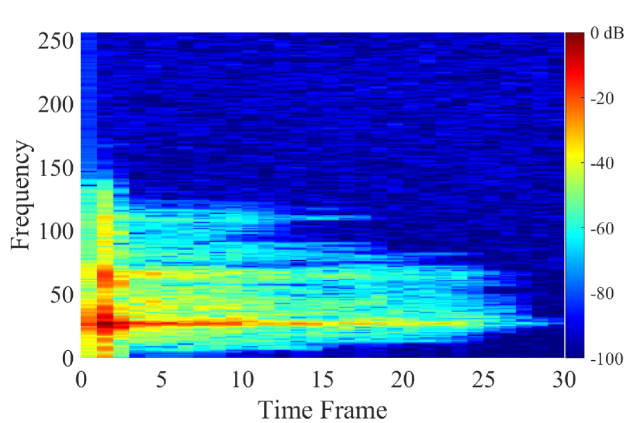
(a) Discrete STFT in (6)

(b) Type-II FUSTFT in (12)

Fig. 1: Power spectrograms of a clicking sound of $0.2$ seconds [32].

4 Two Different Inversions for FUSTFT

4.1 Inversion Based on the Standard Pseudoinverse

Differently from cases of the discrete STFT and FOSTFT, the inversion for FUSTFT is not simple, i.e., the canonical dual window does not exist and the computation process changes dependently on $L_{x}$. In this paper, we realize the inversion by solving the problem similar
to (10). Let $\mathcal{S}:\mathbb{C}^{L_{x}}\to\mathbb{C}^{\frac{L_{w}}{2}\times\left\lceil\frac{L_{x}+L_{w}-\xi}{\xi}\right\rceil}$ be one of the linear mappings (11), (12), and (13). Then the inversion based on the pseudo-inverse is expressed as $(\mathcal{S}^{\mathrm{H}}\circ\mathcal{S})^{-1}\circ\mathcal{S}^{\mathrm{H}}$. In FUSTFT cases, $\mathcal{S}^{\mathrm{H}}\circ\mathcal{S}$ is

$$\setcounter{MaxMatrixCols}{12}\begin{bmatrix}\hskip 4.0pta_{0}&&&\hskip 2.0ptb_{0}&&&&&\\[-2.0pt] &\hskip 3.0pta_{1}&&&b_{1}&&&&&\\[-7.0pt] &&\hskip 3.0pt\ddots&&&\ddots&&&&&\\[-3.0pt] \hskip 4.0ptb_{0}&&&\hskip 2.0pta_{\frac{L_{w}}{2}}&&&b_{\frac{L_{w}}{2}}\\[-6.0pt] &\hskip 3.0ptb_{1}&&&a_{\frac{L_{w}}{2}+1}&&&\ddots\\[-6.0pt] &&\hskip 3.0pt\ddots&&&\ddots&&&\ddots&&&\\[-6.0pt] &&&\hskip 2.0ptb_{\frac{L_{w}}{2}}&&&\ddots&&&\hskip 11.0pt\ddots\\[-6.0pt] &&&&\ddots&&&a_{L_{x}-\frac{L_{w}}{2}-1}&&&b_{L_{x}-\frac{L_{w}}{2}-1}\\[-6.0pt] &&&&&\ddots&&&\ddots\\[-4.0pt] &&&&&&\ddots&&&\hskip 11.0pt\ddots\\[-3.0pt] &&&&&&&b_{L_{x}-\frac{L_{w}}{2}-1}&&&a_{L_{x}-1}\end{bmatrix}$$. (15)

In (15), diagonal components are

$$a_{i}=\frac{L_{w}}{2}\sum_{l=0}^{\left\lceil\frac{L_{w}}{\xi}\right\rceil-1}w^{2}[m_{i}+l\xi]\vspace{-3.4pt}$$ (16)

for all the three types, where $m_{i}=\mathrm{mod}_{\xi}(\hskip 0.25pti+L_{w})$ and $w[\tau]=0$ for $\tau\geq L_{w}$. For Type-I FUSTFT, nonzero nondiagonal components are

$$b_{i}=\frac{L_{w}}{2}\sum_{l=0}^{\left\lceil\frac{L_{w}}{2\xi}\right\rceil-1}w[m_{i}+l\xi]\hskip 0.5ptw[m_{i}+l\xi+\tfrac{L_{w}}{2}]\mbox{.}\vspace{-3.4pt}$$ (17)

For Type-II, each $b_{i}$ is equal to (17) multiplied by $-1$. For Type-III,

$$b_{i}=\frac{L_{w}}{2}\sum_{l=0}^{\left\lceil\frac{L_{w}}{2\xi}\right\rceil-1}(-1)^{\left\lfloor\frac{i+L_{w}-\xi}{\xi}\right\rfloor+l}\hskip 0.5ptw[m_{i}+l\xi]\hskip 0.5ptw[m_{i}+l\xi+\tfrac{L_{w}}{2}]\mbox{.}\vspace{-1pt}$$ (18)

$a_{i}$ in (16) and $b_{i}$ in (17) are periodic with period $\xi$ while $b_{i}$ in (18) is periodic with period $2\xi$. We only have to compute them for one cycle.

For a given complex spectrogram $\bm{X}\in\mathbb{C}^{\frac{L_{w}}{2}\times\left\lceil\frac{L_{x}+L_{w}-\xi}{\xi}\right\rceil}$, define $\bm{y}=:(y[0],y[1],\ldots,y[L_{x}-1])^{\mathrm{T}}:=\mathcal{S}^{\mathrm{H}}(\bm{X})$. Then, the unique solution $\bm{x}$ to a linear system $(\mathcal{S}^{\mathrm{H}}\circ\mathcal{S})\hskip 1.0pt\bm{x}=\bm{y}$ is the inversion result of $\bm{X}$. This linear system is decomposed into $\frac{L_{w}}{2}$ independent systems

$$\begin{bmatrix}a^{\langle i\rangle}_{0}&b^{\langle i\rangle}_{0}&&&\\[0.5pt] b^{\langle i\rangle}_{0}&a^{\langle i\rangle}_{1}&b^{\langle i\rangle}_{1}\\[-4.0pt] &\ddots&\hskip 3.0pt\ddots&\ddots\\[-1.0pt] &&\!\!\hskip 0.5ptb^{\langle i\rangle}_{n_{i}-3}&a^{\langle i\rangle}_{n_{i}-2}&b^{\langle i\rangle}_{n_{i}-2}\\[1.5pt] &&&b^{\langle i\rangle}_{n_{i}-2}&a^{\langle i\rangle}_{n_{i}-1}\end{bmatrix}\begin{bmatrix}x[i]\\[2.0pt] x[i\!+\!\tfrac{L_{w}}{2}]\\[-3.0pt] \vdots\\ x[i\!+\!\tfrac{(n_{i}-2)L_{w}}{2}]\\[2.0pt] x[i\!+\!\tfrac{(n_{i}-1)L_{w}}{2}]\end{bmatrix}=\begin{bmatrix}y[i]\\[2.0pt] y[i\!+\!\tfrac{L_{w}}{2}]\\[-3.0pt] \vdots\\ y[i\!+\!\tfrac{(n_{i}-2)L_{w}}{2}]\\[2.0pt] y[i\!+\!\tfrac{(n_{i}-1)L_{w}}{2}]\end{bmatrix}$$ (19)

($i=0,1,\ldots,\frac{L_{w}}{2}-1$), where $n_{i}=\bigl{\lceil}\frac{2(L_{x}-i)}{L_{w}}\bigr{\rceil}$, $a^{\langle i\rangle}_{j}:=a_{i+j\frac{L_{w}}{2}}$ and
$b^{\langle i\rangle}_{j}:=b_{i+j\frac{L_{w}}{2}}$. Since the matrices in the left side of (19) are tridiagonal matrices, their LU decompositions can be computed in $\mathcal{O}(n)$ [33], and the inversion result $\bm{x}$ is also obtained from $\bm{y}$ in $\mathcal{O}(n)$.

In particular, when $\mathrm{mod}_{\xi}(\frac{L_{w}}{2})=0$ for Type-I and Type-II, or $\mathrm{mod}_{2\xi}(\frac{L_{w}}{2})=0$ for Type-III, we have $a^{\langle i\rangle}_{0}=a^{\langle i\rangle}_{1}=\cdots=a^{\langle i\rangle}_{n_{i}-1}=a_{i}$ and $b^{\langle i\rangle}_{0}=b^{\langle i\rangle}_{1}=\cdots=b^{\langle i\rangle}_{n_{i}-2}=b_{i}$, and hence the matrices in the left side of (19) are tridiagonal Toeplitz matrices. In such cases, the eigenvalues are $\lambda^{\langle i\rangle}_{q}=a_{i}+2b_{i}\cos(\frac{q\pi}{n_{i}+1})>a_{i}-2|b_{i}|>0$ and the eigenvectors are $\bm{u}_{q}=(\sin(\frac{q\pi}{n_{i}+1}),\sin(\frac{2q\pi}{n_{i}+1}),\ldots,\sin(\frac{n_{i}q\pi}{n_{i}+1}))^{\mathrm{T}}\in\mathbb{R}^{n_{i}}$ ($q=1,2,\ldots,n_{i}$) [34]. Therefore, the inversion result $\bm{x}$ is also obtained by using the discrete sine transform (DST) of Type-I [35].

When $\mathrm{mod}_{\xi}(\frac{L_{w}}{2})=0$ and $\mathrm{mod}_{2\xi}(\frac{L_{w}}{2})\neq 0$ for Type-III, we have $b^{\langle i\rangle}_{j}=(-1)^{j}b_{i}$ for all $i$ and $j$. We can also compute the inversion result $\bm{x}$ by using Type-I DST, even in this case, with appropriate sign reversal process (see the actual program in [36] for more detail).

4.2 Inversion Based on the Pseudoinverse with the Periodicity

For Type-I and Type-II, let $p$ be the minimum nonnegative integer s.t. $\mathrm{mod}_{\frac{L_{w}}{2}}(\bigl{\lceil}\frac{L_{x}+L_{w}-\xi}{\xi}\bigr{\rceil}\hskip 0.25pt\xi+p\hskip 1.0pt\xi)=0$. For Type-III, $p$ must also satisfy
$\mathrm{mod}_{2}(\bigl{\lceil}\frac{L_{x}+L_{w}-\xi}{\xi}\bigr{\rceil}+p)=0$. We define $L_{\mathrm{p}}:=\bigl{\lceil}\frac{L_{x}+L_{w}-\xi}{\xi}\bigr{\rceil}\hskip 1.0pt\xi+p\hskip 1.0pt\xi$ and $\bm{x}_{\mathrm{p}}:=(x[0],x[1],\ldots,x[L_{x}-1],x[L_{x}],\ldots,x[L_{\mathrm{p}}-1])^{\mathrm{T}}:=(\bm{x}^{\mathrm{T}},\bm{0}^{\mathrm{T}}_{L_{\mathrm{p}}-L_{x}})^{\mathrm{T}}\in\mathbb{C}^{L_{\mathrm{p}}}$. Let ${\mathcal{S}}_{\mathrm{p}}:\mathbb{C}^{L_{\mathrm{p}}}\to\mathbb{C}^{\frac{L_{w}}{2}\times\left(\left\lceil\frac{L_{x}+L_{w}-\xi}{\xi}\right\rceil+p\right)}$ be a linear mapping, that computes one of (11), (12), and (13) for $l=0,1,\ldots,\bigl{\lceil}\frac{L_{x}+L_{w}-2\xi}{\xi}\bigr{\rceil}+p\hskip 0.5pt$ while assuming the periodic condition, i.e., $x[\tau]=x[L_{\mathrm{p}}\hskip 0.75pt+\hskip 0.75pt\tau]$ for $\tau<0$, according to the convention [6]–[8].

For a given complex spectrogram $\bm{X}\in\mathbb{C}^{\frac{L_{w}}{2}\times\left\lceil\frac{L_{x}+L_{w}-\xi}{\xi}\right\rceil}$, we define $\bm{X}_{\mathrm{p}}:=[\bm{X},\bm{O}_{\frac{L_{w}}{2}\times p\hskip 0.5pt}]\in\mathbb{C}^{\frac{L_{w}}{2}\times\left(\left\lceil\frac{L_{x}+L_{w}-\xi}{\xi}\right\rceil+p\right)}$ and compute the inversion result $\bm{x}_{{}_{\mathrm{p}}}=(\mathcal{S}^{\mathrm{H}}_{\mathrm{p}}\hskip 0.1pt\circ\hskip 0.5pt\mathcal{S}_{\mathrm{p}})^{-1}\hskip 0.1pt\circ\hskip 0.5pt\mathcal{S}^{\mathrm{H}}_{\mathrm{p}}(\bm{X}_{\mathrm{p}})$ of $\bm{X}_{\mathrm{p}}$ under the pe-riodic condition. Then, by extracting the first $L_{x}$ components of $\bm{x}_{\mathrm{p}}$,

we obtain the final inversion result $\bm{x}$ of $\bm{X}$. Therefore, define $\bm{y}_{\mathrm{p}}:=(y[0],y[1],\ldots,y[L_{\mathrm{p}}-1])^{\mathrm{T}}:=\mathcal{S}^{\mathrm{H}}_{\mathrm{p}}(\bm{X}_{\mathrm{p}})$, and we only have to compute the unique solution $\bm{x}_{\mathrm{p}}$ to a linear system $(\mathcal{S}^{\mathrm{H}}_{\mathrm{p}}\circ\mathcal{S}_{\mathrm{p}})\hskip 1.0pt\bm{x}_{\mathrm{p}}=\bm{y}_{\mathrm{p}}$. This is decomposed into $\frac{L_{w}}{2}$ independent systems of the same size

$$\begin{bmatrix}a^{\langle i\rangle}_{0}&b^{\langle i\rangle}_{0}&&&b^{\langle i\rangle}_{n_{i}-1}\\ b^{\langle i\rangle}_{0}&a^{\langle i\rangle}_{1}&b^{\langle i\rangle}_{1}\\[-4.0pt] &\ddots&\hskip 3.0pt\ddots&\ddots\\[-1.0pt] &&\!\!\hskip 0.5ptb^{\langle i\rangle}_{n_{i}-3}&a^{\langle i\rangle}_{n_{i}-2}&b^{\langle i\rangle}_{n_{i}-2}\\[2.0pt] b^{\langle i\rangle}_{n_{i}-1}&&&b^{\langle i\rangle}_{n_{i}-2}&a^{\langle i\rangle}_{n_{i}-1}\end{bmatrix}\begin{bmatrix}x[i]\\[2.0pt] x[i\!+\!\tfrac{L_{w}}{2}]\\[-3.0pt] \vdots\\ x[i\!+\!\tfrac{(n_{i}-2)L_{w}}{2}]\\[2.0pt] x[i\!+\!\tfrac{(n_{i}-1)L_{w}}{2}]\end{bmatrix}=\begin{bmatrix}y[i]\\[2.0pt] y[i\!+\!\tfrac{L_{w}}{2}]\\[-3.0pt] \vdots\\ y[i\!+\!\tfrac{(n_{i}-2)L_{w}}{2}]\\[1.5pt] y[i\!+\!\tfrac{(n_{i}-1)L_{w}}{2}]\end{bmatrix}$$ (20)

($i=0,1,\ldots,\frac{L_{w}}{2}-1$), where $n_{0}=n_{1}=\cdots=n_{\frac{L_{w}}{2}-1}=\frac{2L_{\mathrm{p}}}{L_{w}}$, $a^{\langle i\rangle}_{j}:=a_{i+j\frac{L_{w}}{2}}$, $b^{\langle i\rangle}_{j}:=b_{i+j\frac{L_{w}}{2}}$, and $a_{i}$ and $b_{i}$ are the same as (16), (17), and (18). The matrices in the left side of (20) are periodic tridiagonal matrices, whose LU decompositions are also given in $\mathcal{O}(n)$ [37], and hence $\bm{x}_{\mathrm{p}}$ and the final result $\bm{x}$ are also quickly obtained.

In particular, when $\mathrm{mod}_{\xi}(\frac{L_{w}}{2})=0$ for Type-I and Type-II, or $\mathrm{mod}_{2\xi}(\frac{L_{w}}{2})=0$ for Type-III, we have $a^{\langle i\rangle}_{0}=a^{\langle i\rangle}_{1}=\cdots=a^{\langle i\rangle}_{n_{i}-1}=a_{i}$ and $b^{\langle i\rangle}_{0}=b^{\langle i\rangle}_{1}=\cdots=b^{\langle i\rangle}_{n_{i}-1}=b_{i}$, and hence the matrices in the left side of (20) are symmetric circulant matrices. In such cases, the eigenvalues are $\lambda^{\langle i\rangle}_{q}=a_{i}+2b_{i}\cos(\frac{2q\pi}{n_{i}})\geq a_{i}-2|b_{i}|>0$ and the eigenvectors are $\bm{u}_{q}=(1,e^{-\imath\frac{2q\pi}{n_{i}}},e^{-\imath\frac{4q\pi}{n_{i}}},\ldots,e^{-\imath\frac{2(n_{i}-1)q\pi}{n_{i}}})^{\mathrm{T}}\in\mathbb{C}^{n_{i}}$ ($q=0,1,\ldots,n_{i}-1$). Note that Stanković defined the discrete-time window function as $w[\tau]:=w(\tau\hskip 0.5ptT_{\mathrm{s}})$ in [30], which results in $|b_{i}|=\frac{a_{i}}{2}$ and $\lambda^{\langle i\rangle}_{q}=0$ for $i=\frac{L_{w}}{4}$ when $\xi=\frac{L_{w}}{2}$. On the other hand, we defined it as $w[\tau]:=w((\tau+\frac{1}{2})\hskip 0.25ptT_{\mathrm{s}})$ in this paper, which guarantees $|b_{i}|<\frac{a_{i}}{2}$ and $\lambda^{\langle i\rangle}_{q}>0$ for all $i$. Hence, the inversion result $\bm{x}_{\mathrm{p}}$ is also obtained by using FFT, but we have to note that if $\xi=\frac{L_{w}}{2}$ and $L_{w}$ is relatively large, then $\mathcal{S}^{\mathrm{H}}_{\mathrm{p}}\circ\mathcal{S}_{\mathrm{p}}$ becomes ill-conditioned.

When $\mathrm{mod}_{\xi}(\frac{L_{w}}{2})=0$ and $\mathrm{mod}_{2\xi}(\frac{L_{w}}{2})\neq 0$ for Type-III, we have $b^{\langle i\rangle}_{j}=(-1)^{j}b_{i}$ for all $i$ and $j$. We can also compute the inversion result $\bm{x}_{\mathrm{p}}$ by using FFT, even in this case, with appropriate sign reversal process or appropriate multiplication process by $\imath$ depen-dently on $\mathrm{mod}_{4}(n_{i})$ (see the actual program in [36] for more detail).

4.3 Difference between the Two Inversions for FUSTFT

Many papers explain the discrete STFT under the periodic condition as shown in Sect. 4.2. In the cases of the discrete STFT and FOSTFT, actually both $\mathcal{S}^{\mathrm{H}}\circ\mathcal{S}$ and $\mathcal{S}^{\mathrm{H}}_{\mathrm{p}}\circ\mathcal{S}_{\mathrm{p}}$ are diagonal matrices whose diagonal components are periodic, and the two inversion results are always the same. As a result, there is almost no problem even if we explain the discrete STFT and FOSTFT without the periodic condition.

On the other hand, in the case of FUSTFT, these two inversions have different properties. Define $\mathcal{R}:=\{\bm{X}\in\mathbb{C}^{\frac{L_{w}}{2}\times\left\lceil\frac{L_{x}+L_{w}-\xi}{\xi}\right\rceil}\,|$ $\exists\bm{x}\hskip 0.1858pt\in\hskip 0.1858pt\mathbb{C}^{L_{x}}\,\hskip 0.2858pt\bm{X}\hskip 0.1858pt=\hskip 0.1858pt\mathcal{S}(\bm{x})\}$  as  the  range  of  FUSTFT  $\mathcal{S}$.  For  a  complex

spectrogram $\bm{X}\in\mathcal{R}$, both inversions can recover $\bm{x}$ s.t. $\bm{X}=\mathcal{S}(\bm{x})$. For $\bm{X}\not\in\mathcal{R}$, the standard inversion $(\mathcal{S}^{\mathrm{H}}\circ\mathcal{S})^{-1}\circ\mathcal{S}^{\mathrm{H}}$ can recover the most consistent $\bm{x}$ with $\bm{X}$, while the inversion $(\mathcal{S}^{\mathrm{H}}_{\mathrm{p}}\circ\mathcal{S}_{\mathrm{p}})^{-1}\circ\mathcal{S}^{\mathrm{H}}_{\mathrm{p}}$ in the periodic condition can recover the most consistent $\bm{x}_{\mathrm{p}}$ with $\bm{X}_{\mathrm{p}}$, which means that the last $L_{\mathrm{p}}-L_{x}$ components of $\bm{x}_{\mathrm{p}}$ become non-zero. It might seem that the former inversion $(\mathcal{S}^{\mathrm{H}}\circ\mathcal{S})^{-1}\circ\mathcal{S}^{\mathrm{H}}$ should always be used, but the latter inversion $(\mathcal{S}^{\mathrm{H}}_{\mathrm{p}}\circ\mathcal{S}_{\mathrm{p}})^{-1}\circ\mathcal{S}^{\mathrm{H}}_{\mathrm{p}}$ has a special property in the case of $\xi=\frac{L_{w}}{2}$. Only when $\xi=\frac{L_{w}}{2}$, $\mathcal{S}_{\mathrm{p}}$ becomes a non-redundant transform, and $\bm{x}_{\mathrm{p}}$ s.t. $\bm{X}_{\mathrm{p}}=\mathcal{S}_{\mathrm{p}}(\bm{x}_{\mathrm{p}})$ can be always recovered by the latter inversion. As a result, for any complex spectrogram $\bm{X}\not\in\mathcal{R}$, a discrete-time signal $\bm{x}$ that guarantees the perfect consistency other than the first and last frames is always recovered.

Table 1: Inversion results $\hat{\bm{x}}$ from $\bm{X}\in\mathcal{R}$ which is inside the range.

$L_{w}$	$\xi$	Inverse	$\frac{\lVert\bm{x}-\hat{\bm{x}}\rVert_{2}}{\lVert\bm{x}\rVert_{2}}$	$\frac{\lVert\bm{X}-\mathcal{S}(\hat{\bm{x}})\rVert_{\mathrm{F}}}{\lVert\bm{X}\rVert_{\mathrm{F}}}$	$\begin{aligned} \mbox{}\\[-10.0pt] \tfrac{\lVert\bm{X}-\mathcal{S}(\hat{\bm{x}})\rVert^{\mathrm{int}}_{\mathrm{F}}}{\lVert\bm{X}\rVert_{\mathrm{F}}^{\mathrm{int}}}\end{aligned}$
$\begin{aligned} \mbox{}\\[-4.5pt] 2{,}048\end{aligned}$	$\frac{L_{w}}{2}$	$\begin{aligned} \mbox{}\\[-8.5pt] \mathcal{S}\\[-10.0pt] \mbox{}\end{aligned}$	$5.0\times 10^{-14}$	$8.3\times 10^{-16}$	$8.3\times 10^{-16}$
		$\begin{aligned} \mbox{}\\[-9.0pt] \mathcal{S}_{\mathrm{p}}\\[-9.0pt] \mbox{}\end{aligned}$	$1.0\times 10^{-13}$	$3.8\times 10^{-15}$	$9.6\times 10^{-16}$
	$\frac{L_{w}}{8}$	$\begin{aligned} \mbox{}\\[-8.0pt] \mathcal{S}\\[-10.0pt] \mbox{}\end{aligned}$	$6.5\times 10^{-16}$	$6.7\times 10^{-16}$	$6.7\times 10^{-16}$
		$\begin{aligned} \mbox{}\\[-9.0pt] \mathcal{S}_{\mathrm{p}}\\[-9.0pt] \mbox{}\end{aligned}$	$4.7\times 10^{-16}$	$5.1\times 10^{-16}$	$5.1\times 10^{-16}$
$\begin{aligned} \mbox{}\\[-4.5pt] 8{,}192\end{aligned}$	$\frac{L_{w}}{2}$	$\begin{aligned} \mbox{}\\[-8.5pt] \mathcal{S}\\[-10.0pt] \mbox{}\end{aligned}$	$1.3\times 10^{-14}$	$5.7\times 10^{-16}$	$5.7\times 10^{-16}$
		$\begin{aligned} \mbox{}\\[-9.0pt] \mathcal{S}_{\mathrm{p}}\\[-9.0pt] \mbox{}\end{aligned}$	$1.8\times 10^{-12}$	$1.1\times 10^{-13}$	$9.8\times 10^{-16}$
	$\frac{L_{w}}{8}$	$\begin{aligned} \mbox{}\\[-8.0pt] \mathcal{S}\\[-10.0pt] \mbox{}\end{aligned}$	$4.4\times 10^{-16}$	$5.1\times 10^{-16}$	$5.1\times 10^{-16}$
		$\begin{aligned} \mbox{}\\[-9.0pt] \mathcal{S}_{\mathrm{p}}\\[-10.0pt] \mbox{}\end{aligned}$	$\begin{aligned} \mbox{}\\[-9.75pt] 4.4\times 10^{-16}\end{aligned}$	$\begin{aligned} \mbox{}\\[-9.75pt] 5.0\times 10^{-16}\end{aligned}$	$\begin{aligned} \mbox{}\\[-9.75pt] 5.0\times 10^{-16}\end{aligned}$

Table 2: Inversion results $\hat{\bm{x}}$ from $\widehat{\bm{X}}\not\in\mathcal{R}$ which is outside the range.

$L_{w}$	$\xi$	Inverse	$\frac{\lVert\bm{x}-\hat{\bm{x}}\rVert_{2}}{\lVert\bm{x}\rVert_{2}}$	$\frac{\lVert\widehat{\bm{X}}-\mathcal{S}(\hat{\bm{x}})\rVert_{\mathrm{F}}}{\lVert\widehat{\bm{X}}\rVert_{\mathrm{F}}}$	$\begin{aligned} \mbox{}\\[-10.0pt] \tfrac{\lVert\widehat{\bm{X}}-\mathcal{S}(\hat{\bm{x}})\rVert^{\mathrm{int}}_{\mathrm{F}}}{\lVert\widehat{\bm{X}}\rVert_{\mathrm{F}}^{\mathrm{int}}}\end{aligned}$
$\begin{aligned} \mbox{}\\[-4.5pt] 2{,}048\end{aligned}$	$\frac{L_{w}}{2}$	$\begin{aligned} \mbox{}\\[-8.5pt] \mathcal{S}\\[-10.0pt] \mbox{}\end{aligned}$	$2.9\times 10^{-2}$	$6.0\times 10^{-4}$	$2.5\times 10^{-4}$
		$\begin{aligned} \mbox{}\\[-9.0pt] \mathcal{S}_{\mathrm{p}}\\[-9.0pt] \mbox{}\end{aligned}$	$3.5\times 10^{-2}$	$1.2\times 10^{-3}$	$1.7\times 10^{-15}$
	$\frac{L_{w}}{8}$	$\begin{aligned} \mbox{}\\[-8.0pt] \mathcal{S}\\[-10.0pt] \mbox{}\end{aligned}$	$8.0\times 10^{-3}$	$1.3\times 10^{-2}$	$1.3\times 10^{-2}$
		$\begin{aligned} \mbox{}\\[-9.0pt] \mathcal{S}_{\mathrm{p}}\\[-9.0pt] \mbox{}\end{aligned}$	$8.0\times 10^{-3}$	$1.3\times 10^{-2}$	$1.3\times 10^{-2}$
$\begin{aligned} \mbox{}\\[-4.5pt] 8{,}192\end{aligned}$	$\frac{L_{w}}{2}$	$\begin{aligned} \mbox{}\\[-8.5pt] \mathcal{S}\\[-10.0pt] \mbox{}\end{aligned}$	$2.7\times 10^{-2}$	$1.6\times 10^{-3}$	$4.2\times 10^{-4}$
		$\begin{aligned} \mbox{}\\[-9.0pt] \mathcal{S}_{\mathrm{p}}\\[-9.0pt] \mbox{}\end{aligned}$	$6.9\times 10^{-2}$	$4.5\times 10^{-3}$	$1.1\times 10^{-14}$
	$\frac{L_{w}}{8}$	$\begin{aligned} \mbox{}\\[-8.0pt] \mathcal{S}\\[-10.0pt] \mbox{}\end{aligned}$	$8.0\times 10^{-3}$	$1.4\times 10^{-2}$	$1.3\times 10^{-2}$
		$\begin{aligned} \mbox{}\\[-9.0pt] \mathcal{S}_{\mathrm{p}}\\[-10.0pt] \mbox{}\end{aligned}$	$\begin{aligned} \mbox{}\\[-9.75pt] 8.0\times 10^{-3}\end{aligned}$	$\begin{aligned} \mbox{}\\[-9.75pt] 1.4\times 10^{-2}\end{aligned}$	$\begin{aligned} \mbox{}\\[-9.75pt] 1.3\times 10^{-2}\end{aligned}$

We confirm the properties of the inversions in Sects. 4.1 and 4.2 for Type-II FUSTFT. A sound signal $\bm{x}$ of $15$ seconds is transformed into a complex spectrogram $\bm{X}\in\mathcal{R}$, and we create a noisy version $\widehat{\bm{X}}\not\in\mathcal{R}$ by adding complex white Gaussian noise of variance $10^{-6}$ to $\bm{X}$. The performance of the inversion results $\hat{\bm{x}}$ from $\bm{X}$ and $\widehat{\bm{X}}$ are summarized in Tables 1 and 2, respectively. From these tables, we can confirm that both inversions work correctly. In particular, when $\xi=\frac{L_{w}}{2}$, the inversion results by $(\mathcal{S}^{\mathrm{H}}_{\mathrm{p}}\circ\mathcal{S}_{\mathrm{p}})^{-1}\circ\mathcal{S}^{\mathrm{H}}_{\mathrm{p}}$ demonstrated the

slight numerical instability in blue letters of Table 1 and the perfect consistency other than the first and last frames in red letters of Table 2.

5 Conclusion

This paper proposed FUSTFT and its two inversions. FUSTFT gives efficient spectrogram matrices by computing only half the frequency components of the discrete STFT. By using FUSTFT, it is expected that window functions of relatively large $L_{w}$ such as the Kaiser window and the truncated Gaussian window will be easier to use. Since we can arbitrarily modify magnitudes and phases other than the first and last frames when $\xi=\frac{L_{w}}{2}$, further development of spectrogram-based techniques is also expected. There is also a possibility that flexible transforms such as Type-III FUSTFT will find new applications.

References

• [1] M. R. Portnoff, “Implementation of the digital phase vocoder using the fast Fourier transform,” IEEE Trans. Acoust. Speech Signal Process., vol. 24, no. 3, pp. 243–248, 1976.
• [2] J. B. Allen, “Short term spectral analysis, synthesis, and modification by discrete Fourier transform,” IEEE Trans. Acoust. Speech Signal Process., vol. 25, no. 3, pp. 235–238, 1977.
• [3] J. B. Allen and L. R. Rabiner, “A unified approach to short-time Fourier analysis and synthesis,” Proc. IEEE, vol. 65, no. 11, pp. 1558–1564, 1977.
• [4] R. E. Crochiere, “A weighted overlap-add method of short-time Fourier analysis/synthesis,” IEEE Trans. Acoust. Speech Signal Process., vol. 28, no. 1, pp. 99–102, 1980.
• [5] L. Cohen, Time-Frequency Analysis: Theory and Applications.    Englewood Cliffs, NJ: Prentice Hall, 1994.
• [6] H. G. Feichtinger and T. Strohmer, Eds., Gabor Analysis and Algorithms: Theory and Applications.    Secaucus, NJ: Birkhäuser, 1997.
• [7] K. Gröchenig, Foundations of Time-Frequency Analysis.    Secaucus, NJ: Birkhäuser, 2001.
• [8] H. G. Feichtinger and T. Strohmer, Eds., Advances in Gabor Analysis.    Secaucus, NJ: Birkhäuser, 2002.
• [9] P. L. Søndergaard, “Finite discrete Gabor analysis,” Ph.D. thesis, Technical University of Denmark, 2007.
• [10] K. Yatabe, Y. Masuyama, T. Kusano, and Y. Oikawa, “Representation of complex spectrogram via phase conversion,” Acoust. Sci. & Tech., vol. 40, no. 3, pp. 170–177, 2019.
• [11] H. S. Malvar, “Lapped transforms for efficient transform/sub-band coding,” IEEE Trans. Acoust. Speech Signal Process., vol. 38, no. 6, pp. 969–978, 1990.
• [12] I. Daubechies, S. Jaffard and J. Journé, “A simple Wilson orthonormal basis with exponential decay,” SIAM J. Math. Anal., vol. 22, no. 2, pp. 554–573, 1991.
• [13] H. Bölcskei, G. Feichtinger, K. Gröchenig, and F. Hlawatsch, “Discrete-time Wilson expansions,” in Proc. TFTS, Paris, 1996, pp. 525–528.
• [14] H. S. Malvar, “A modulated complex lapped transform and its applications to audio processing,” in Proc. ICASSP, Phoenix, AZ, 1999, pp. 1421–1424.
• [15] J. C. Brown, “Calculation of a constant-Q spectral transform,” J. Acoust. Soc. Am., vol. 89, no. 1, pp. 425–434, 1991.
• [16] I. Daubechies, Ten Lectures on Wavelets, ser. CBMS-NSF Regional Conference Series in Applied Mathematics.    Philadelphia, PA: SIAM, 1992, vol. 61.
• [17] J. J. Benedetto and M. W. Frazier, Wavelets: Mathematics and Applications, ser. Studies in Advanced Mathematics.    Boca Raton, FL: CRC Press, 1993, vol. 13.
• [18] G. Kaiser, A Friendly Guide to Wavelets.    Secaucus, NJ: Birkhäuser, 2011.
• [19] V. Verfaille, U. Zolzer, and D. Arfib, “Adaptive digital audio effects (A-DAFx): A new class of sound transformations,” IEEE Transactions on Audio, Speech, and Language Processing, vol. 14, no. 5, pp. 1817–1831, 2006.
• [20] G. Yu, S. Mallat, and E. Bacry, “Audio denoising by time-frequency block thresholding,” IEEE Trans. on Signal Process., vol. 56, no. 5, pp. 1830–1839, 2008.
• [21] E. Benetos, S. Dixon, D. Giannoulis, H. Kirchhoff, and A. Klapuri, “Automatic music transcription: challenges and future directions,” J. Intel. Inf. Syst., vol. 41, no. 3, pp. 407–434, 2013.
• [22] M. Mauch, C. Cannam, R. Bittner, G. Fazekas, J. Salamon, J. Dai, J. Bello, and S. Dixon, “Computer-aided melody note transcription using the Tony software: accuracy and efficiency,” in Proc. TENOR, Paris, 2015, pp. 28–30.
• [23] T. Fujiwara, M. Yamagishi, and I. Yamada, “Reduced-rank modeling of time-varying spectral patterns for supervised source separation,” in Proc. ICASSP, Brisbane, 2015, pp. 3307–3311.
• [24] Y. Wakabayashi and N. Ono, “Griffin–Lim phase reconstruction using short-time Fourier transform with zero-padded frame analysis,” in Proc. APSIPA ASC, Lanzhou, 2019, pp. 1863–1867.
• [25] Y. Takahashi, D. Kitahara, K. Matsuura, and A. Hirabayashi, “Determined source separation using the sparsity of impulse responses,” in Proc. ICASSP, Barcelona, 2020, pp. 686–690.
• [26] R. Nakatsu, D. Kitahara, and A. Hirabayashi, “Non-Griffin–Lim type signal recovery from magnitude spectrogram,” in Proc. ICASSP, Barcelona, 2020, pp. 791–795.
• [27] T. Werther, Y. C. Eldar, and N. K. Subbanna, “Dual Gabor frames: theory and computational aspects,” IEEE Trans. Signal Process., vol. 53, no. 11, pp. 4147–4158, 2005.
• [28] B. Yang, “A study of inverse short-time Fourier transform,” in Proc. ICASSP, Las Vegas, NV, 2008, pp. 3541–3544.
• [29] I. Daubechies, A. Grossmann, and Y. Meyer, “Painless nonorthogonal expansions,” J. Math. Phys., vol. 27, no. 5, pp. 1271–1283, 1986.
• [30] L. Stanković, “On the STFT inversion redundancy,” IEEE Trans. Circuits Syst. II: Express Briefs, vol. 63, no. 3, pp. 284–288, 2016.
• [31] S. Moreno-Picot, F. J. Ferri, M. Arevalillo-Herráez, and W. Díaz-Villanueva, “Efficient analysis and synthesis using a new factorization of the Gabor frame matrix,” IEEE Trans. Signal Process., vol. 66, no. 17, pp. 4564–4573, 2018.
• [32] MathWorks, “Modified discrete cosine transform: MATLAB mdct.” https://www.mathworks.com/help/audio/ref/mdct.html
• [33] L. H. Thomas, “Elliptic problems in linear differential equations over a network,” Watson Sci. Comput. Lab. Report, Columbia Univ., 1949.
• [34] S. Noschese, L. Pasquini, and L. Reichel, “Tridiagonal Toeplitz matrices: properties and novel applications,” Numer. Linear Algebra Appl., vol. 20, no. 2, pp. 302–326, 2013.
• [35] S. A. Martucci, “Symmetric convolution and the discrete sine and cosine transforms,” IEEE Trans. Signal Process., vol. 42, no. 5, pp. 1038–1051, 1994.
• [36] D. Kitahara, The MATLAB program of FUSTFT, https://lab.d-kitahara.com/codes/
• [37] M. M. Chawla and R. R. Khazal, “A parallel elimination method for “periodic” tridiagonal systems,” Int. J. Comput. Math., vol. 79, no. 4, pp. 473–484, 2002.