Deep Learning for Individual Heterogeneity: An Automatic Inference Framework

Abstract

We develop methodology for estimation and inference using machine learning to enrich economic models. Our framework takes a standard economic model and recasts the parameters as fully flexible nonparametric functions, to capture the rich heterogeneity based on potentially high dimensional or complex observable characteristics. These “parameter functions” retain the interpretability, economic meaning, and discipline of classical parameters. In contrast to common implementations of machine learning in economics, these functions need not be predictions. We show that deep learning is particularly well-suited to structured modeling of heterogeneity in economics. First, we show how the network architecture can be easily designed to match the global structure of the economic model, delivering novel methodology that moves deep learning beyond prediction. Second, we prove convergence rates for the estimated parameter functions. These parameter functions are then the key input into the finite-dimensional parameter of inferential interest. We obtain valid inference based on a novel orthogonal score or influence function calculation that covers any second-stage parameter and any machine-learning-enriched model that uses a smooth per-observation loss function. No additional derivations are required and the score can be taken directly to data, using automatic differentiation if needed to obtain the components: the researcher need only define the original model and define the parameter of interest. A key insight is that we need not write down the influence function in order to evaluate it on the data. We apply this after deep learning, but our result can be used for any first-step estimator. Our framework covers, as special cases, well-known examples such as average treatment effects and partially linear models, but we also seamlessly deliver new results for such diverse examples as price elasticities, willingness-to-pay, and surplus measures in binary or multinomial choice models, average marginal and partial effects of continuous treatment variables, fractional outcome models, count data, heterogeneous production function components, and more. Across all these contexts inference can be made as automated as is currently available in special cases. We illustrate the utility of our framework with an application to a large scale advertising experiment for short-term loans. We show how economically meaningful estimates and inferences can be made that would be unavailable without our framework.

Keywords: Deep Learning, Influence Functions, Neyman Orthogonality, Heterogeneity, Structural Modeling, Semiparametric Inference

1 Introduction

The goal of this paper is to leverage modern machine learning and rich data to capture individual heterogeneity in the context of economic models. Parametric, structural models are a cornerstone of applied research in economics and social sciences. The parameters estimated in these models are interpretable, useful for policy, and disciplined by economic principles. We develop a methodology to maintain these advantages while simultaneously incorporating machine learning methods for flexibly estimating heterogeneity. Our idea is to recast the parameters of a model as flexible functions themselves: enriching the model without losing the structure. We estimate the parameters using deep learning, for which we provide new results. We then deliver second-step inference by deriving a novel influence function that applies to any such enriched model.

The starting point is a researcher-specified model that relates outcomes $\bm{Y}$ to the covariates of central interest, the policy or treatment variables $\bm{T}$. This model is encapsulated by a loss function $\ell(\bm{Y},\bm{T},\bm{\theta})$ for a vector of parameters $\bm{\theta}$ that are estimated from the data. The model encodes structure that is grounded in economic principles and economic reasoning. To fix ideas, take the context of our empirical application where we revisit the data of Bertrand et al. (2010). Here $\bm{Y}$ is a customer’s binary choice to apply for a loan and $\bm{T}$ are characteristics of the loan and an advertisement received, one of which is the interest rate offered. A standard approach to this problem would be a (structural) logistic binary choice model where the parameters $\bm{\theta}$ are the coefficients on $\bm{T}$, including an intercept. Such a model has numerous advantages. First, the parameters have a clear and direct interpretation, and generally respect economic theory. Second, economically meaningful, and policy-relevant, summary parameters are easily computed, such as elasticities or measures of surplus. Further, the economic structure can be used to answer substantial policy questions. For example, although interest rates are only observed at certain values, we can use the model to study what would occur at other levels. Indeed, from basic economic principles like profit maximization, we can compute the optimal interest rate as a function of the parameters, say $r^{*}(\bm{\theta})$. All of these are only possible because of the economic structure imposed on the analysis.

However, if there is heterogeneity, which is almost a given in most contexts, the parameter estimates may not be reliable in practice, and this has spurred a push to move beyond rigid parametric models, which can only crudely capture heterogeneity, if at all. Heterogeneity can come in many forms or depend on many things. This fact, along with the increasing availability of large, complex data sets, has motivated the adoption of novel machine learning methods in economics, allowing researchers to study economic phenomena at levels of detail previously not possible.

Our approach to this problem allows for the use of powerful machine learning to capture rich heterogeneity, while simultaneously maintaining the structure and interpretability of the economic model, with all its advantages. To do this, we recast the model’s parameters as functions of observed characteristics $\bm{X}$, thus enriching the model to $\ell(\bm{Y},\bm{T},\bm{\theta}(\bm{X}))$. These “parameter functions” allow for fully flexible heterogeneity but keep intact the structure of the economic model connecting $\bm{Y}$ and $\bm{T}$. In general we will not know either the functional form of $\bm{\theta}_{0}(\bm{x})$ nor which covariates are important. This is one strong motivation for applying modern machine learning methods. Our approach exploits the flexibility of machine learning within the structure dictated by economic models.

We thus deploy machine learning to directly estimate meaningful objects, which has several advantages compared to using ML to only obtain predictions. First, for any set of characteristics $\bm{X}=\bm{x}$, $\bm{\theta}(\bm{x})$ gives the effect for an individual of “type” $\bm{x}$, and therefore retains all of the meaning, interpretability and usefulness of the original parameters. Additionally, we can “score” or “type” future individuals through their characteristics, because $\bm{\theta}(\bm{x})$ captures heterogeneity that can be used for future policy. Second, because we have maintained the economic model, we can leverage its structure to answer substantive questions. For example, in our data we can compute the personalized, targeted optimal interest rate $r^{*}(\bm{\theta}(\bm{x}))$.

Our approach of implementing ML by enriching an economic model thus directly address several major drawbacks of common applications of ML in economics. Typically, ML have largely been confined to prediction problems, or those that can be convert to prediction problems. These prediction functions are added to models only as nuisance functions. The term “nuisance” here is illustrative: it connotes that flexibility is required in some piece of the model, but is not per se interesting or meaningful. This is typical not just of ML, but of semiparametrics more broadly, and we aim to depart from this mindset. In the context of our application, for example, this might mean using ML to classify potential borrowers with an unstructured function $\mathbb{E}[Y|\bm{t},\bm{x}]=\theta(\bm{T},\bm{X})$: a pure prediction problem. Such an estimate would not only have worse statistical properties, it would lose the economic meaning of the original model. The results would not be interpretable directly and useful quantities would be difficult or impossible to extract. Further, without the discipline of the economic principles of the model, such estimates may make little sense.

To implement our approach we require estimates of the parameter functions $\bm{\theta}(\bm{x})$ and an inference engine for second-stage parameters of interest. We gives results for both steps. In both cases we make heavy use of the idea that we have enriched an economic model: it is this concrete structure that enables us to deliver broad and powerful results. For first stage estimation, we show that deep neural networks (DNNs) have a unique combination of strengths which makes them able to directly incorporate the structure of the economic model as well as handle modern data sets and complex heterogeneity. We prove new convergence rates in this context. For second step inference we give a new orthogonal score that can be widely and easily applied.

Deep neural networks have had incredible empirical success, matching or setting the state of the art in a wide range of tasks. But this has largely been in prediction problems, and indeed, most software is designed only to optimize prediction loss functions. We develop a novel, yet simple, architectural idea so that the global structure of the economic model is baked into the estimation directly and the parameter functions are recovered, instead of focusing on prediction. The idea is simple and implementation is straightforward, but this appears to have been mostly overlooked in the ML literature. Our ideas are in the vein of nonparametric M-estimation, which has a longer history but has relied on classical methods which are not equipped to handle the complex heterogeneity that is the hallmark of modern applications. DNNs also handle discrete data seamlessly in practice (as well as in theory), in contrast to classical methods. We prove new results for structured deep neural network estimates of $\bm{\theta}(\bm{X})$, which crucially recover the parameter functions, not predictions, and depend on the dimension of $\bm{X}$, the heterogeneity, independent of the dimension of the variables of interest $\bm{T}$. Our results build on the recent work of Farrell et al. (2021) and contribute more broadly to the nonparametric M-estimation literature (see Chen (2007) for review and references).

Next, a feasible inference engine is required following the deep learning of $\bm{\theta}(\bm{X})$ in the enriched model. We obtain valid inference on a finite-dimensional parameter of interest $\bm{\mu}$ that depends directly on the parameter functions $\bm{\theta}(\bm{X})$. We achieve this by characterizing an influence function, or orthogonal score, for $\bm{\mu}$, and then making use of the recent results for influence function based estimators following machine learning. Our derivation builds directly on long-standing ideas in semiparametrics, chiefly Newey (1994), and for inference we follow the method of Chernozhukov et al. (2018), combining an orthogonal score with sample splitting. A drawback of this general approach to semiparametric inference is that the influence function must be known in advance, and this has perhaps hampered take-up among applied researchers. Most applications focus on a few special cases where the influence function is known (e.g. the case of average treatment effects). Our contribution to inference is to derive a single influence function that includes the correction term for any smooth per-observation loss $\ell(\bm{Y},\bm{T},\bm{\theta}(\bm{X}))$. Thus, for any ML-enriched economic model inference can proceed without further calculations. We apply this after deep learning, but our influence function can be used in general, for any first step estimator meeting standard conditions, such as lasso, trees and forests, or classical sieve or kernel methods. Our influence functions recovers well known special cases such as average treatment effects and partially linear models, but immediately delivers new results for many other contexts, including selection models, choice models, fractional outcomes, and more broadly, smooth QMLE contexts and other such areas.

A key insight is that we only need to characterize the influence function and evaluate its empirical analogue at each data point, consequently obtaining a point estimator and standard errors, without needing to explicitly write it down. This can be contrasted with the typical approach of writing down the influence function, or orthogonal score, explicitly and then plugging in estimates of each nuisance function. Our goal is to make inference feasible in a wide variety of settings, not to focus on the properties of the score, such as efficiency comparisons, and this shift of mindset allows for broadly applicable methodology. An important tool here is automatic differentiation. The influence function depends only upon ordinary derivatives of the model $\ell$ and of the function defining the parameter of interest, as though the model were still parametric with homogeneous effects. In many cases, the derivatives of the model are already well known, and these forms can be used, but if not, the derivatives can be evaluated on the data automatically. For example, recall that in our empirical study, $r^{*}(\bm{\theta}(\bm{x}))$ is the personalized optimal interest rate. This $r^{*}(\bm{\theta}(\bm{x}))$ is not available in closed form, but rather as the solution to a fixed point problem. Therefore, the influence function for a parameter such as expected profits at the optimal personalized interest rates $\mu=\mathbb{E}[\pi(r^{*}(\bm{\theta}(\bm{X})))]$ cannot be explicitly written down. Nonetheless, because $\mu$ is a smooth function of $r^{*}(\bm{\theta})$, and $r^{*}(\bm{\theta})$ depends smoothly on $\bm{\theta}$, its derivatives can be evaluated at each data point with no trouble, allowing feasible inference. This would not be possible without our approach that retains the economic structure of the model.

Taken together, the combination of the specification we adopt, the availability of computing infrastructure, and the theory we present, offers a perfect package for applied researchers across economics and social science hoping to exploit ML but maintain discipline-specific knowledge and interpretability. Our work should be broadly useful by delivering a tractable and valid estimation and inference framework that covers many interesting contexts. The next section presents an overview of our methodological framework and its interpretation, and gives a brief overview of the main results. Our results related to many strands of recent literature, and we discuss these in context as they arise. Section 3 shows how deep learning is an excellent tool in our context and gives theoretical results. Section 4 discusses semiparametric inference, our novel influence function, and asymptotic normality. We apply our methods in Section 5 to an empirical study of short term loan applications. Section 6 gives a sense of the breadth of applicability of our results by discussing a number of examples, but is by no means exhaustive. Extensions are discussed in Section 7 and finally Section 8 concludes. Proofs are given in the appendix.

2 A Methodological Framework for Enriching Economic Models with Machine Learning

In this section we describe our framework enriching economic models to capture individual heterogeneity and give an informal summary of our results. The starting point is a standard, parametric economic model. We assume the researcher observes data on outcomes, $\bm{Y}\in\mathbb{R}^{d_{\bm{Y}}}$, and on the covariates of central interest, or treatments, $\bm{T}\in\mathbb{R}^{d_{\bm{T}}}$, which can be continuous, discrete, or mixed. The researcher relates these two with an economic model, which is encapsulated by a parametric per-observation loss function, $\ell(\bm{Y},\bm{T},\bm{\theta})$, indexed by a parameter $\bm{\theta}\in\mathbb{R}^{d_{\bm{\theta}}}$. For some parameter space $\bm{\Theta}$, dictated by the structure of the problem, the researcher then solves $\min_{\bm{\theta}\in\bm{\Theta}}\mathbb{E}[\ell(\bm{Y},\bm{T},\bm{\theta})]$, that is, standard M-estimation, including all (psuedo-/quasi-) likelihood-like settings. Two key aspects of this approach are: (i) $\bm{\theta}$ are parameters, not predictions, and have economic meaning and (ii) the effects are homogeneous. We will retain (i) while removing (ii).

Our framework starts with the same parametric model, but recasts the parameters $\bm{\theta}$ as functions of observed individual characteristics $\bm{X}\in\mathbb{R}^{d_{\bm{X}}}$ to allow for heterogeneity. Thus, in place of $\bm{\theta}$ we will have $\bm{\theta}(\bm{x})$, mapping $\mathbb{R}^{d_{\bm{X}}}\mapsto\mathbb{R}^{d_{\bm{\theta}}}$, and we assume that the true parameter functions $\bm{\theta}_{0}(\cdot)$ solve

$$\bm{\theta}_{0}(\cdot)=\operatorname*{arg\,min}_{\bm{\theta}\in\mathcal{H}}\mathbb{E}\left[\ell\big{(}\bm{Y},\bm{T},\bm{\theta}(\bm{X})\big{)}\right],$$ (2.1)

for an appropriate function class $\mathcal{H}$ (formalities are given below). We can thus capture heterogeneity in a fully flexible way, while retaining all the structure and interpretability of the standard model. For intuition, it is often useful to remember that at any value $\bm{X}=\bm{x}$, $\bm{\theta}(\bm{x})$ has the same interpretation as $\bm{\theta}$, but for the “type” determined by $\bm{x}$. It is also useful to think of individual-specific effects, which may be what researchers are implicitly worried about when heterogeneity is a concern, that is $\bm{\theta}_{i}$ minimizes $\ell(\bm{y}_{i},\bm{t}_{i},\bm{\theta})$ for each $i$. Such individual specific parameters are also as interpretable and meaningful as the original, homogeneous case, but of course $\bm{\theta}_{i}$ cannot typically be recovered from the data, and may not be useful in the future, as person $i$ will not be seen again. One can think of $\bm{\theta}(\bm{x}_{i})$ as an approximation to $\bm{\theta}_{i}$, one that uses all available information, and thus captures the portion of heterogeneity useful for future policy targeting.

Figure 1: Illustration of the deep neural network estimation of the parameter functions $\bm{\theta}(\bm{x})$ for a generic structured model (2.1)

The functions $\bm{\theta}(\bm{x})$ are not prediction functions necessarily, nor do we view them as nuisance functions, a term which implies they are uninteresting. Section 3 shows why deep learning is well suited for structured modeling and gives a novel, yet simple architectural idea for doing so. This means that we use deep learning to recover meaningful functions, thus moving ML away from prediction tasks and toward estimation of scientifically and economically interesting objectives, a shift in mindset from the typical applications of machine learning. This implementation innovation and the convergence rates for the resulting estimated parameter functions are the two main contributions of this paper to deep learning, and to machine learning first stage parameters more broadly.

The key result is that we estimate the parameter functions at a fast enough rate for inference, and importantly, that the rate depends only upon the number of continuous heterogeneity covariates, denoted $d_{C}\leq d_{\bm{X}}$, and does not depend on dimension of the policy/treatment variables. That is, for our estimator $\bm{\widehat{\theta}}$ of $\bm{\theta}_{0}(\bm{x})$ defined by (2.1), Theorem 1 establishes that

$$\Big{\|}\widehat{\theta}_{k}-\theta_{0k}\Big{\|}^{2}_{L_{2}(\bm{X})}=O(n^{-\frac{p}{p+d_{C}}}\log^{8}(n)),\qquad\quad k=1,\ldots,d_{\bm{\theta}},$$

provided $\ell$ is sufficiently smooth and curved near the truth. This result relies on our novel architectural idea, where the structure of the model is baked directly into the deep net architecture. The architecture, and hence the optimization of the loss, targets the parameter functions, not predictions. This idea is illustrated in Figure 1.

The heterogeneous parameter functions $\bm{\theta}_{0}(\bm{x})$ are then key inputs into the final parameter of inferential interest, denoted $\bm{\mu}_{0}\in\mathbb{R}^{d_{\bm{\mu}}}$. For a known, smooth function $H:\{\mathbb{R}^{d_{\bm{X}}}\times\mathbb{R}^{d_{\bm{\theta}}}\}\mapsto\mathbb{R}^{d_{\bm{\mu}}}$, chosen by the researcher, we conduct inference on

$$\bm{\mu}_{0}=\mathbb{E}\Big{[}\bm{H}(\bm{X},\bm{\theta}_{0}(\bm{X});\bm{t}^{*})\Big{]},$$ (2.2)

where $\bm{t}^{*}$ is some fixed value of interest. Many economically interesting statistics take this form, in particular, depending on functions that are not predictions. To make inference feasible we derive an influence function for any such $\bm{\mu}_{0}$, which includes deriving the correction factor for any ML-enriched M-estimation problem. Regularity conditions are below; in particular, we assume the $\bm{\mu}_{0}$ is pathwise differentiable. Beyond this, the form of $\bm{\mu}_{0}$ can be generalized at the cost of notation.

The main theoretical contribution to second stage inference is the influence function calculation, yielding a Neyman orthogonal score, that is specific enough to be directly implemented while still being general enough to cover any enriched structural model based on a smooth per-observation loss function. From a practical point of view, two key ideas in our work are the use of computational differentiation (automatic or numerical) and the conceptual point of evaluating influence functions on the observed data rather than writing them down.

Theorem 2, in Section 4, gives the Neyman orthogonal score for any (sufficiently regular) such parameter $\bm{\mu}_{0}$ and first stage $\bm{\theta}(\bm{x})$ coming from an ML-enriched model. Importantly, this score depends only on ordinary derivatives. Let $\bm{H}_{\bm{\theta}}(\bm{x},\bm{\theta}(\bm{x});\bm{t}^{*})$ and $\bm{\ell}_{\bm{\theta}}(\bm{y},\bm{t},\bm{\theta}(\bm{x}))$ be the gradients of $H$ and $\ell$ with respect to $\bm{\theta}$ and denote $\bm{\Lambda}(\bm{x})=\mathbb{E}[\bm{\ell}_{\bm{\theta}\bm{\theta}}(\bm{y},\bm{t},\bm{\theta}(\bm{x}))\mid\bm{X}=\bm{x}]$ the conditional expectation of the Hessian of $\ell$, all evaluated at $\bm{\theta}=\bm{\theta}(\bm{x})$. Then the Neyman orthogonal score is $\bm{\psi}(\bm{y},\bm{t},\bm{x},\bm{\theta},\bm{\Lambda})-\bm{\mu}_{0}$, where

$$\bm{\psi}(\bm{y},\bm{t},\bm{x},\bm{\theta},\bm{\Lambda})=\bm{H}\left(\bm{x},\bm{\theta}(\bm{x});\bm{t}^{*}\right)-\bm{H}_{\bm{\theta}}(\bm{x},\bm{\theta}(\bm{x});\bm{t}^{*})\bm{\Lambda}(\bm{x})^{-1}\bm{\ell}_{\bm{\theta}}(\bm{w},\bm{\theta}(\bm{x})).$$

This can be taken to the data directly. That is, given estimators $\bm{\widehat{\theta}}$ and $\widehat{\bm{\Lambda}}$, we can evaluate $\bm{\psi}(\bm{y}_{i},\bm{t}_{i},\bm{x}_{i},\bm{\widehat{\theta}},\widehat{\bm{\Lambda}})$ at every data point without further derivation, which is all that is required for feasible estimation and inference. For many standard models, these derivatives are known. If not, they can obtained using automatic differentiation tools or other computational methods. In other words, once the researcher specifies their economic model via $\ell(\bm{y},\bm{t},\bm{\theta})$ and parameter of interest via $\bm{H}$, the full influence function is known and ready to use. This holds for any sufficiently smooth functions, even if not available in closed form, as in our example with the optimal interest rate and corresponding profits.

The general form of this orthogonal score and what each piece represents conceptually should call to mind the parametric case. If $\bm{\theta}_{0}$ were constant, then classical results for two-step estimation, as in Newey and McFadden (1994, Section 6), would yield the effect of the first stage on the second, and deliver an influence function that looks the same, but with $\bm{H}_{\bm{\theta}}$ and $\bm{\Lambda}$ as constants, instead of conditional on $\bm{x}$. Thus our influence function result can be viewed as establishing the analogous result for fully nonparametric parameter functions. We view this familiarity as a strength, as it perfectly matches our core idea of enriching a well-understood economic model, and may help to demystify semiparametric inference.

Armed with this orthogonal score, we can obtain a point estimator $\bm{\widehat{\mu}}$ and standard errors $\bm{\widehat{\Psi}}$ such that $\bm{\widehat{\mu}}\stackrel{{\scriptstyle d}}{{\sim}}\mathcal{N}(\mu_{0},\bm{\widehat{\Psi}}/n)$, allowing inference on any aspect of the vector $\bm{\mu}_{0}$. For example, if $d_{\bm{\mu}}=1$ so the parameter of interest is a scalar,

$$\left[\widehat{\mu}-1.96\sqrt{\widehat{\Psi}/n}\ ,\ \widehat{\mu}+1.96\sqrt{\widehat{\Psi}/n}\right]$$

is a valid 95% confidence interval. Obtaining this inference in practice is no more difficult than what is currently available for simple cases, like average treatment effects: we estimate the two nonparametric objects, $\bm{\widehat{\theta}}$ and $\widehat{\bm{\Lambda}}$, and plug them in as needed. Estimation of $\bm{\Lambda}(\bm{x})$ is discussed in more detail below, and can rely on standard ML methods, including deep learning, and may require sample splitting. However, an important methodological point is that when $\bm{T}$ is randomized this matrix can often be computed, as opposed to estimated. In general, two-step semiparametric inference often involves a denominator term such as this, and computing this term can yield more stable and robust results compared estimating it. See Remark 4 and our application in Section 5.

A special case of our framework that is useful for illustrating the main ideas, as well as prevalent in empirical and theoretical work, is when $\bm{Y}$ is a scalar $Y$ and (2.1) is built around conditional mean restriction and the parameters are the intercept and the slopes. That is, let $\bm{t}$ include a constant term and assume that for a known function $G(u),u\in\mathbb{R}$,

$$\mathbb{E}[Y\mid\bm{X}=\bm{x},\bm{T}=\bm{t}]=G\left(\bm{\theta}_{0}(\bm{x})^{\prime}\bm{t}\right).$$ (2.3)

Recall that the $\bm{X}$ are observed; this is not a random coefficient model. Rather, we have made the intercept and slope fully heterogeneous in observables. Clearly, (2.3) can be implemented using (2.1), given an appropriate loss function. A crucial piece will be the first order condition of that loss, that is, what orthogonality condition to use. For example, if $G$ is the logistic link we may take $\ell$ to be the nonlinear least squares or the likelihood, which have different first order conditions, and this will change the influence function given later and thus impact implementation. O’Hagan (1978) may be the earliest treatment of a model like (2.3), and the structure here is often known as a “varying coefficient” model (Cleveland et al., 1991; Hastie and Tibshirani, 1993), “functional coefficient” model (Chen and Tsay, 1993), or “smooth coefficient” model (Li et al., 2002), and falls into the class of “extended linear models” as in Stone et al. (1997). Our results speak directly to this literature and to additive models, where $\mathbb{E}[Y\mid\bm{X}=\bm{x}]=G(\theta_{01}(\bm{x}_{1})+\theta_{02}(\bm{x}_{2}))$, for non-overlapping subsets $\bm{x}_{1},\bm{x}_{2}$ of $\bm{x}$, we will obtain rates for $\theta_{01}(\bm{x}_{1})$ and $\theta_{02}(\bm{x}_{2})$.

The form of Equation (2.3) makes clear that our approach is to enrich a parametric relationship between the outcomes $\bm{Y}$ and policy variables $\bm{T}$, rather than restrict a fully nonparametric (prediction) model. It is better to view $G(\bm{\theta}_{0}(\bm{x})^{\prime}\bm{t})$ as an ML-enriched version of $\mathbb{E}[Y\mid\bm{T}=\bm{t}]=G(\bm{\theta}_{0}^{\prime}\bm{t})$ instead of as a restricted version of the a prediction model such as $\mathbb{E}[Y\mid\bm{X}=\bm{x},\bm{T}=\bm{t}]=\theta_{0}(\bm{x},\bm{t})$, which would be more typical of ML.

This distinction is both practically and theoretically important. Again, consider the binary choice model of our application. In our framework, the heterogeneous interest rate (price) effect is directly available as a coefficient function. Compare this to the unstructured prediction case: to recover the same conceptual quantity one would first estimate the prediction function $\mathbb{E}[Y\mid\bm{X}=\bm{x},\bm{T}=\bm{t}]=\theta_{0}(\bm{x},\bm{t})$ and then obtain the derivative with respect to the rate variable $R$ (an element of $\bm{T}$), that is, $\mathbb{E}[\partial\theta_{0}(\bm{x},\bm{T})/\partial R|\bm{X}=\bm{x}]$. This is possible, but cumbersome, and inference on the average may not be regular without weighting (see also Section 6.3). It would be difficult or impossible to recover measures such as elasticities or optimal prices. However, with our structural model, all of these are simple and automatic.

3 Structured Deep Learning for Parameter Functions

We now discuss in detail the deep neural network (DNN) estimation of the parameter functions $\bm{\theta}_{0}(\bm{x})$ and state our theoretical results for the first stage. DNNs have a unique combination of strengths which makes them an excellent choice, among machine learning methods, for recovering individual heterogeneity. The most obvious argument for deep learning is the incredible success DNNs have had across a wide variety of learning problems, in research applications and real-world use. They have been found to handle many different tasks and data types extremely well. In many applications the dimension of $\bm{X}$ is large enough, and the heterogeneity complex enough, that classical methods will not work, but deep learning still yields excellent results. See Goodfellow et al. (2016) for a textbook treatment and Farrell et al. (2021) for recent literature and further introduction.

The primary use of DNNs has been for prediction, and much of the statistical study has been restricted to this case. We take DNNs beyond prediction, and use them to learn the (structural) parameter functions $\bm{\theta}_{0}(\bm{x})$. To do so, we design a new architecture, shown in Figure 1, to measure the loss directly in terms of the parameter functions. The key idea is to decouple the final loss and the functions to be learned: we use DNNs to approximate the parameter functions $\bm{\theta}_{0}(\bm{x})$ in a penultimate “parameter layer”, and these are then combined according to the economic model in the final, “model layer” of the network. This is crucial because it forces the machine learning to be faithful to the economic structure and it allows us to learn the components of $\bm{\theta}_{0}(\bm{x})$, which are of direct interest and required for learning $\bm{\mu}$. To approximate the functions we use standard fully-connected feedforward networks (multi-layer perceptrons, MLPs) and the rectified linear unit (ReLU) activation function.

This change, from $\theta$ to $\theta(\bm{X})$ is simple, yet powerful. It allows for deep learning of individual heterogeneity on any interesting parameter function. These functions may be coefficients that ultimately go into a prediction, as in Equation (2.3), variances or covariances, or other parameters of the original model. To make this formal, let $\mathcal{F}_{\rm DNN}$ be a class of ReLU-DNNs that is restricted to our structured architecture, and also yields $\|\theta_{k}\|_{\infty}$ bounded. We then obtain $\bm{\widehat{\theta}}$ by solving the empirical analogue of (2.1),

$$\bm{\widehat{\theta}}=\operatorname*{arg\,min}_{\bm{\theta}\in\mathcal{F}_{\rm DNN}}\frac{1}{n}\sum_{i=1}^{n}\ell\left(\bm{y}_{i},\bm{t}_{i},\bm{\theta}(\bm{x}_{i})\right).$$ (3.1)

DNNs are not the only possible method that can be used, nor do we claim any formal optimality for them. Having said that, from a practical point of view, they are ideal for several reasons. First, we are able to easily and transparently make our estimator mirror the global structure of the model because DNNs learn a basis-function style representation, and in this way are akin to a global smoother. More apt for the present purpose, we dub this property “structural compatibility”. This makes the machine learning faithful to the economics, rather than allowing the reverse. Although it is possible to embed “local” methods, such as kernel-based (Fan and Zhang, 2008) or tree-based (Zeileis et al., 2008; Athey et al., 2019; Chatla and Shmueli, 2020) estimators, doing so with DNNs is simple, transparent, and tractable, and as the economic model holds globally, we may wish to match this in estimation. Second, like tree-based methods, DNNs handle discrete covariates automatically, including fully flexible interactions. We do not need to restrict attention, in practice or in theory, to continuous $\bm{X}$. In nonparametric theory there is often no penalty in the rate of convergence for discrete variables (under standard assumptions), but realizing these gains in practice can be difficult, as most nonparametric estimators are designed with continuous variables in mind (such as those built upon basis expansions or kernel approximations). DNNs require no customization: the inputs shown in Figure 1 can be any mix of continuous and discrete data. By exploiting our structured architecture, we prove that only the dimension of the continuous elements of $\bm{X}$, the heterogeneity, affects the rates of convergence of our DNN estimators, neither discrete covariates nor $d_{\bm{T}}$ impact the rate.

The handling of discrete covariates is a major advantage over classical sieve methods or methods that select series terms, such as the lasso. Classical methods are ill-equipped to handle modern complex, high-dimensional tasks, and, in practice, variable selection methods require pre-specifying the functional forms and interactions over which to search. However, such methods are structurally compatible in our sense, and our results contribute directly to the large body of work on nonparametric M-estimation (see Chen (2007) discussion and further references). Setting our methodology and theory apart from earlier work is that we explicitly advocate the enrichment of a standard structural model, relating $\bm{Y}$ and $\bm{T}$, rather than starting with a fully generic case. The more common starting point in semi- or nonparametric M estimation and inference would be a model such as $\ell\left(\bm{y}_{i},\bm{t}_{i},\bm{x}_{i},\bm{\mu},\bm{\theta}(\cdot)\right)$, instead of our explicit enriched model and two step approach. Our approach is what allows us to deliver concrete, fully implementable results. Extensions to more general settings would be a useful future step, however.

Finally, it is worth mentioning that other recent work has considered the combination of deep learning and some form of structural modeling (examples include Wei and Jiang, 2019; Igami, 2020; Kaji et al., 2020; Chen et al., 2021). Typically, the goal is estimation of a parametric structural model and deep learning methods are applied to learn the mapping of data to parameters. Our focus, using deep learning to estimate individual-level heterogeneity, is quite different, and further, we give theoretical results on deep neural network estimation and subsequent inference which are not available in prior work. Babii et al. (2020) combine economics with prediction-focused machine learning, where economic reasoning is used to support assymetric in classification loss functions. This is another interesting avenue for merging economics with machine learning.

3.1 Convergence for Structured Deep Neural Networks

We now state our theoretical results for DNN estimation of the parameter functions $\bm{\theta}_{0}(\bm{x})$. We will give a generic result, which necessarily requires high level conditions, and then illustrate more concrete ideas in the case of the slope and intercept parameter functions. The results in this section contribute to the recent literature on the statistical properties of deep learning and to the longer tradition of sieve M estimation. Our assumptions and results are reminiscent of both.

We require two sets of conditions: one covers the model $\ell(\bm{y},\bm{t},\bm{\theta}(\bm{x}))$ and one gives regularity for $(\bm{Y},\bm{X}^{\prime},\bm{T}^{\prime})^{\prime}$ and $\bm{\theta}_{0}(\bm{x})$. For the loss function, we require Lipschitz continuity in general and, near the truth, sufficient curvature. Neither are restrictive and both are common in the nonparametric M estimation literature (cf Chen (2007) and others, where further references and use of other norms are discussed). These conditions are for estimation of $\bm{\theta}_{0}(\bm{x})$; further assumptions will be required for inference.

Assumption 1.

Suppose that $\bm{\theta}_{0}(\bm{x})$ are nonparametrically identified in (2.1), uniformly bounded, and that there are constants $c_{1}$, $c_{2}$, and $C_{\ell}$ that are bounded and bounded away from zero, such that

$$|\ell(\bm{y},\bm{t},\bm{\theta}(\bm{x}))-\ell(\bm{y},\bm{t},\bm{\tilde{\theta}}(\bm{x})|\leq C_{\ell}\|\bm{\theta}(\bm{x})-\bm{\tilde{\theta}}(\bm{x})\|_{2},$$

$$c_{1}\mathbb{E}\left[\|\bm{\theta}(\bm{X})-\bm{\theta}_{0}(\bm{X})\|_{2}^{2}\right]\leq\mathbb{E}[\ell(\bm{Y},\bm{T},\bm{\theta}(\bm{X}))]-\mathbb{E}[\ell(\bm{Y},\bm{T},\bm{\theta}_{0}(\bm{X}))]\leq c_{2}\mathbb{E}\left[\|\bm{\theta}(\bm{X})-\bm{\theta}_{0}(\bm{X})\|_{2}^{2}\right].$$

The curvature requirement will often be implied by restrictions on the Hessian or on the matrix $\bm{\Lambda}(\bm{x})$. Such restrictions are natural in our setting, as they will be required for inference anyway, and are known to hold in many contexts. Some potentially interesting cases are ruled out, such as quantile regression. Modifications to our theory could allow for these cases: for example, Padilla et al. (2020) apply the methods of Farrell et al. (2021) to quantile regression.

Let $\bm{W}=(\bm{Y}^{\prime},\bm{T}^{\prime},\bm{X}^{\prime})^{\prime}$ be the population random variables, with an observation denoted $\bm{w}_{i}=(\bm{y}_{i}^{\prime},\bm{t}_{i}^{\prime},\bm{x}_{i}^{\prime})^{\prime}$. Let $\bm{X}_{C}$ denote the continuously distributed elements of $\bm{X}$, and define $d_{C}=\dim(\bm{X}_{C})$, and take the rest to be binary random variables, without loss of generality. Part (iii) of this assumption restricts to smooth functions, which are known to be approximable by deep neural networks Yarotsky (2017, 2018); Hanin (2017).

Assumption 2.

(i) the elements of $\bm{W}$ are bounded random variables. (ii) $\bm{X}_{C}$ has compact connected support, taken to be $[-1,1]^{d_{C}}$. (iii) As functions of $\bm{x}_{C}$, the continuously distributed components of $\bm{X}$, $\theta_{0k}(\bm{x})\in\mathcal{W}^{p,\infty}([-1,1]^{d_{C}})$, for $k=1,\ldots,d_{\bm{\theta}}$, where for positive integers $p$ and $q$, define the Hölder ball $\mathcal{W}^{p,\infty}([-1,1]^{q})$ of functions $h:\mathbb{R}^{q}\to\mathbb{R}$ with smoothness $p\in\mathbb{N}_{+}$ as

$$\mathcal{W}^{p,\infty}([-1,1]^{q}):=\left\{h:\max_{\bm{r},|\bm{r}|\leq p}\operatorname*{ess\,sup}_{\bm{v}\in[-1,1]^{q}}|D^{\bm{r}}h(\bm{v})|\leq 1\right\},$$

where $\bm{r}=(r_{1},\ldots,r_{q})$, $|\bm{r}|=r_{1}+\ldots+r_{q}$ and $D^{\bm{r}}h$ is the weak derivative.

We now have the following result, proven in the appendix. Here we focus on smooth functions as well as the commonplace deep and wide multi-layer perceptrons (fully connected, feedforward neural networks). In the appendix, we give a more general result, one that is agnostic about the type of approximation, and hence the type of network. For example, the general results can be used to obtain faster rates or cover fixed-width, very deep networks (Farrell et al., 2021, Section 2.3).

Theorem 1.

Let $\bm{w}_{i}$, $i=1,\ldots,n$, be a random sample that obeys Assumptions 1 and 2. For $\bm{\widehat{\theta}}$ solving (3.1), with $\mathcal{F}_{\rm DNN}$ structured according to Figure 1, with width $H\asymp n^{(d_{C})/2(p+d_{C})}\log^{2}n$ and depth $L\asymp\log n$, it holds that

$$\|\widehat{\theta}_{k}-\theta_{0k}\|^{2}_{L_{2}(\bm{X})}\leq C\cdot\left\{n^{-\frac{p}{p+d_{C}}}\log^{8}n+\frac{\log\log n}{n}\right\}$$

and

$$\mathbb{E}_{n}\left[\left(\widehat{\theta}_{k}-\theta_{0k}\right)^{2}\right]\leq C\cdot\left\{n^{-\frac{p}{p+d_{C}}}\log^{8}n+\frac{\log\log n}{n}\right\}$$

for $n$ large enough with probability $1-\exp\{n^{-\frac{d_{C}}{p+d_{C}}}\log^{8}n\}$, for $k=1,\ldots,d_{\bm{\theta}}$, where the constant $C$ may depend on the dimensions $\bm{W}$, $d_{\bm{\theta}}$, and other fixed quantities in Assumptions 1 and 2.

The result of Theorem 1 speaks directly to the nonparametric M estimation literature. It shows that deep nets enjoy the same properties of other methods, but has the advantages discussed above. A theoretical drawback is that for a given smoothness level, this rate is not optimal. It is however sufficiently fast for inference and reflects the excellent empirical performance. This theorem fully takes deep learning away from prediction and toward learning economically meaningful parameters.

The conditions of Theorem 1 are necessarily high level, giving the generality of the setting. Verying these conditions in a given setting is required, but is often straightfoward. Importantly, because we are specifically focusing on enriching a parametric model, familiar analyses from the parametric case can aid in interpreting the conditions required. For example, our conditions are the natural analogues of what is required in well-understood QMLE problems, and the intuition from these can be ported directly.

Figure 2: Illustration of the deep neural network estimation of the parameter functions $\bm{\theta}(\bm{x})$ for a generic structured model (2.3)

To illustrate, return to the regression-type model of (2.3), where the model is $\mathbb{E}[Y\mid\bm{X}=\bm{x},\bm{T}=\bm{t}]=G(\bm{\theta}_{0}(\bm{x})^{\prime}\bm{t})$ and $\bm{t}$ includes a constant term. The final loss in this case still revolves around prediction (beit a QMLE or nonlinear least squares), but our architectural idea is still important, because we need to learn the slope and intercept functions separately. This is shown in Figure 2. That figure also illustrates how our results apply immediately to generalized additive models, where the different components of $\bm{\theta}_{0}$ are known to rely on different subsets of $\bm{X}$: we simply sever the appropriate links, so that separate networks feed into the parameter layer nodes.

For this model we can also illustrate the verification of the high level conditions with familiar, primitive assumptions in this case.

Assumption 3.

(i) The conditional expectation $G(\bm{\theta}_{0}(\bm{x})^{\prime}\bm{t})$ enters the loss through a known, real-valued transformation $g(\cdot)$, where (i) $g$ and $G$ are continuously invertible and $g/\|g\|_{\infty}$ and $G/\|G\|_{\infty}$ belong to $\mathcal{W}^{p,\infty}([-1,1])$, for $p\geq 3$. (ii) Assumption 1 holds with $\ell(\bm{y},\bm{t},\bm{\theta}(\bm{x}))$ replaced by $\ell(\bm{y},g)$, and the conditions therein apply to the scalar argument $g$. (iii) The eigenvalues of $\mathbb{E}[\bm{T}\bm{T}^{\prime}\mid\bm{X}=\bm{x}]$ are bounded and bounded away from zero uniformly in $\bm{x}$.

Condition (i) ensures that the loss function is sufficiently smooth while (ii) and (iii) ensures the curvature through the standard positive variance condition. These conditions are familiar from the parametric case. For example, consider condition (iii) in the original model $\mathbb{E}[Y\mid\bm{T}=\bm{t}]=G(\bm{\theta}_{0}^{\prime}\bm{t})$. In such a model, the assumption that $\mathbb{E}[\bm{T}\bm{T}^{\prime}]$ is positive definite would be standard. Leaning on the intuition that the enriched model is akin to running the original model for each $\bm{X}=\bm{x}$, we see the condition is exactly what would be expected. Versions of these assumptions are also required in the semiparametric models that are special cases of $\mathbb{E}[Y\mid\bm{X}=\bm{x},\bm{T}=\bm{t}]=G(\bm{\theta}_{0}(\bm{x})^{\prime}\bm{t})$, including treatment effects and partially linear models, as in Section 6.

These assumptions are sufficient for identification of the slope and intercept functions in this case. A similar verification should be done for other models, and may lean on prior work in parametric M estimation, as discussed for several cases in Section 6. Specializing Theorem 1 to this case, we have the following result.

Corollary 1.

Let the conditions of Theorem 1 and Assumption 3 hold. Then for a DNN structured according to Figure 2, $\|\widehat{\theta}_{k}-\theta_{0k}\|_{L_{2}(\bm{X})}^{2}=O(n^{-\frac{p}{p+d_{C}}}\log^{8}(n))$, for $k=1,\ldots,d_{\bm{\theta}}$, and $\|G(\bm{\widehat{\theta}}(\bm{x})^{\prime}\bm{t})-G(\bm{\theta}_{0}(\bm{x})^{\prime}\bm{t})\|_{L_{2}(\bm{X})}^{2}=O(n^{-\frac{p}{p+d_{C}}}\log^{8}(n))$.

Here we give two results. First, we show that we can estimate the heterogeneous intercept and slope parameters at the appropriate rate, depending on the dimension of the heterogeneity. This is direct from Theorem 1. This is required as economic constructs depend on these parameters, rather than on the conditional expectation $\mathbb{E}[Y|\bm{x},\bm{t}]$ as a whole.

We also state a result for estimating the regression function $\mathbb{E}[Y|\bm{x},\bm{t}]$ in the structural model (2.3). From a statistical point of view, this result establishes that structured DNNs have excellent performance in varying coefficient models, additive models, and other such cases, and therefore may be of independent interest. It is also useful for comparing to the more typical use of inference after ML, where the (prediction) function $\mathbb{E}[Y|\bm{x},\bm{t}]$ would be unstructured. The key feature to note is that the convergence rate depends only on the dimension of (the continuous component of) $\bm{X}$, not $d_{\bm{T}}$. Even if the final inference relies on conditional expectations, or if the parameter functions could be obtained from the unstructured predictions, naive estimation of these would give a much slower rate, dependent on $d_{\bm{X}}+d_{\bm{T}}-1$ (since $\bm{T}$ includes an intercept). This would often be too slow for subsequent inference. For example, in our empirical illustration this would require 22 dimensional nonparametrics, which may be prohibitively high even for deep learning, and if the goal is to recover a measure of “linear” impact, such as a treatment effect, marginal effect, or other average derivative, an unnecessary complication.

That the rate depends only on $d_{\bm{X}}$ is intuitively exactly what should happen: the heterogeneity is where the model is flexible. In our case, this result is due to our structured architecture, Figures 1 and 2, and not adaptive estimation. The model structure is enforced, not recovered. Certain specialized types of DNNs may in fact adapt to such structures (Bach, 2017; Bauer and Kohler, 2019; Schmidt-Hieber, 2019). First, this is not useful for our purposes because $\bm{\theta}_{0}(\bm{x})$ cannot be recovered. Second, experience has shown that imposing the structure of the model (2.1) improves estimation quality when the structure exists to allow for adaptivity.

For other recent theoretical results on deep learning in other contexts, see Liang (2018), Polson and Ročková (2018), Wang and Ročková (2020), Liang and Tran-Bach (2020), and references therein as well as in Farrell et al. (2021). One important aspect we do not address is regularization, neither the implicit regularization that may occur in the optimization nor explicit regularization of the network parameters themselves though norm penalties, weight decay, drop out, or other methods. In our applications we obtain excellent performance without using explicit regularization, though in low signal-to-noise scenarios adding explicit regularization to the implicit regularization may yield improvements, and has been shown to be optimal in an adversarial game with nature (Blanchet et al., 2020). The role of regularization, its implementation, and its consequences for estimation and subsequent inference, are major open questions for deep learning.

4 Influence Function and Semiparametric Inference

With the framework in place and estimates of the parameter functions in hand, we now turn to estimation and inference for $\bm{\mu}_{0}=\mathbb{E}[\bm{H}(\bm{X},\bm{\theta}_{0}(\bm{X});\bm{t}^{*})]$ from (2.2). The key contribution here, given in Theorem 2, is a novel Neyman orthogonal score for any such $\bm{\mu}_{0}$, given any model (2.1). Importantly, this score can be immediately taken to data, without additional derivations. Our framework is simultaneously general enough to cover a large number of settings, yet specific enough that the influence function can be fully characterized. As is standard, the orthogonal score depends on $\bm{\theta}_{0}(\bm{x})$ and a second nonparametric object, but the latter piece is also fully characterized and is therefore estimable without additional work. With this score, we can apply the methods and results of Chernozhukov et al. (2018) to immediately obtain asymptotic Normality. This is spelled out in Section 4.2 below.

4.1 Influence Function

Obtaining valid semiparametric inference does not require basing the estimation framework on an influence function (or Neyman orthogonal, doubly robust, or locally robust, scores). The major appeal of these methods is that we can obtain valid distributional approximations under weaker conditions on the first stage estimates, i.e., on how well $\bm{\widehat{\theta}}$ recovers $\bm{\theta}_{0}$. These weaker conditions are known to hold for many ML methods, and in particular Section 3 shows that they hold for deep learning. In other words, it is useful to view the influence function as a tool for obtaining feasible inference, rather than being of direct interest itself, for efficiency considerations or other comparisons. This viewpoint is implicit in much recent work on inference after ML (e.g., Belloni et al., 2014; Farrell, 2015; Chernozhukov et al., 2018) but it is worthwhile to make it explicit to better understand how thinking this way greatly expands the breadth of what we can cover, including cases like the optimal interest rate, which cannot be given in closed form. The same motivation is explicit in the recent work on “auto-DML”, where the necessary pieces of the influence function are estimated from the data, and are thus need not be derived at all (Chernozhukov et al., 2020c, b; Chernozhukov et al., 2020a; Chernozhukov et al., 2020d; Chernozhukov et al., 2021). Our focus on interpretable parameter functions rather than regression functions distinguishes our setting from this line of work, which manifests in two central ways: (i) our first stage is more general, as we do not focus on regressions; (ii) our inference targets are broader in some ways, given the flexibility of the first stage, but we require $\bm{\theta}_{0}$ to enter through evaluation at $\bm{X}$, ruling out examples such as integrals across data points.

Influence functions have a long history in econometrics. Newey (1994) remains the seminal treatment. We defer to that work and Ichimura and Newey (2015) for more background, including regularity conditions for existence of an influence function. Perhaps the most well known and commonly used influence function is that for average treatment effects, which we recover as a special case in Example 6.1. The history of this influence function is illustrative: it was characterized precisely first for the purposes of efficiency considerations (Hahn, 1998, 2004), later used to show certain plug-in estimators could be efficient (Hirano et al., 2003; Imbens et al., 2007), and finally only recently used for post-ML inference to exploit the weaker conditions (Farrell, 2015). The partially linear model (Section 6.3) is another standard example and followed a similar trajectory, most imporantly for our discussion being the first setting where inference was proven (uniformly) valid after variable selection (Belloni et al., 2014).

In both cases, the influence function was first derived and then its components estimated directly. This exercise has been repeated in numerous models for numerous parameters (see Section 6, and lists in Ichimura and Newey (2015) or Chernozhukov et al. (2020a)). In a sense, we follow this path: derive the correction factor for any setting in Section 2, obeying the regularity conditions below. However, our correction factor covers many settings, as we take advantage of the structure of the original model in the derivation. Thus, in any of these settings, inference is now as straightforward as it is for average treatment effects: two nonparametric pieces must be estimated, and these are combined into the orthogonal score, with sample splitting if needed. That is, we can follow the recipe of Chernozhukov et al. (2018). We broaden the application of these ideas and show how they work even in cases where we use automatic differentiation to obtain the piece of the score and the parameter of interest is not available in closed form. That is, we can still evaluate the influence function estimator, given below, on the data points. And so, while deriving correction terms for estimation is somewhat standard, or results are novel in their broad applicability. Our influence function nests many cases from the literature and delivers new results.

Our end result will reflect the core idea behind our framework: enriching a standard model by converting the parameters to parameter functions. In purely parametric two-step models, without heterogeneity, the influence function of the first step parameters themselves can be used to adjust the second step (Newey and McFadden, 1994, Section 6). Our result is the nonparametric generalization of this, and one strength of the result is this familiarity, which will aid in practice by making assumptions transparent and familiar and by guiding implementation.

To state the result, we will in fact require the gradient and Hessian of $\ell$, defined via ordinary differentiation. Let $\bm{\ell}_{\bm{\theta}}(\bm{w},\bm{\theta}(\bm{x}))$ be the $d_{\bm{\theta}}$-vector of first derivatives,

$$\bm{\ell}_{\bm{\theta}}(\bm{y},\bm{t},\bm{\theta}(\bm{x}))=\left.\frac{\partial\ell\big{(}\bm{y},\bm{t},\bm{b}\big{)}}{\partial\bm{b}}\right|_{\bm{b}=\bm{\theta}(\bm{x})},$$ (4.1)

and $\bm{\ell}_{\bm{\theta}\bm{\theta}}(\bm{y},\bm{t},\bm{\theta}(\bm{x}))$ as the $d_{\bm{\theta}}\times d_{\bm{\theta}}$ matrix of second derivatives, that is with $\{k_{1},k_{2}\}$ element given by

$$\Big{[}\bm{\ell}_{\bm{\theta}\bm{\theta}}(\bm{y},\bm{t},\bm{\theta}(\bm{x}))\Big{]}_{k_{1},k_{2}}=\left.\frac{\partial^{2}\ell\left(\bm{y},\bm{t},\bm{b}\right)}{\partial b_{k_{1}}\partial b_{k_{2}}}\right|_{\bm{b}=\bm{\theta}(\bm{x})},$$ (4.2)

where $b_{k_{1}}$ and $b_{k_{2}}$ are the respective elements of the place-holder $\bm{b}$. The use of standard differentiation in these contexts has been used in some prior work.

We can now state our assumptions and give the main result of this section, the form of the orthogonal score. Our assumptions are mostly standard and ensure sufficient regularity for our influence function to be calculated and asymptotic normality obtained by resulting estimator. One conceptually important point is that in general these conditions are not sufficient for a causal interpretation, which will require some form of unconfoundedness or conditional exogeneity (as in Examples 6.1 or 6.3).

Assumption 4.

The following conditions hold on the distribution of $\bm{W}=(Y,\bm{X}^{\prime},\bm{T}^{\prime})^{\prime}$, uniformly in the given conditioning elements. (i) Equation (2.1) holds and identifies $\bm{\theta}_{0}(\bm{x})$, where $\ell(\bm{w},\bm{\theta})$ is thrice continuously differentiable with respect to $\bm{\theta}$. (ii) $\mathbb{E}[\left.\bm{\ell}_{\bm{\theta}}(\bm{Y},\bm{t},\bm{\theta}(\bm{x}))\right|\bm{X}=\bm{x},\bm{T}=\bm{t}]=0$. (iii) For $\bm{\ell}_{\bm{\theta}\bm{\theta}}$ of (4.2), $\bm{\Lambda}(\bm{x}):=\mathbb{E}[\left.\bm{\ell}_{\bm{\theta}\bm{\theta}}(\bm{Y},\bm{T},\bm{\theta}(\bm{x}))\right|\bm{X}=\bm{x}]$ is invertible with bounded inverse. (iv) The parameter $\bm{\mu}_{0}$ of Equation (2.2) is identified and pathwise differentiable and $\bm{H}$ is thrice continuously differentiable in $\bm{\theta}$. (v) $\bm{H}(\bm{x},\bm{\theta}_{0}(\bm{x});\bm{t}^{*})$ and $\bm{\ell}_{\bm{\theta}}(\bm{y},\bm{t},\bm{\theta}(\bm{x}))$ possess $q>4$ finite absolute moments and positive variance.

The most important assumptions here are that the first order condition of (2.1) holds and that $\bm{\mu}_{0}$ is pathwise differentiable. The latter keeps focus on semiparametric contexts. The former follows our idea to take a well-defined parametric model, for which such identification would hold, and enrich the model with machine learning. Of course not all models of the form (2.1) will be so identified, and this must be verified.

For intuition, consider the case of the conditional mean restriction (2.3) where simple sufficient conditions can be stated. Many loss functions yield $\bm{\ell}_{\bm{\theta}}(\bm{w},\bm{\theta}(\bm{x}))=\bm{t}(G(\bm{\theta}(\bm{x})^{\prime}\bm{t})-y)$, in which case $\bm{\Lambda}(\bm{x})=\mathbb{E}[\dot{G}\bm{T}\bm{T}^{\prime}\mid\bm{X}=\bm{x}]$, with $\dot{G}$ the derivative of $G$ with respect to its scalar argument, evaluated at the index $\bm{\theta}_{0}(\bm{x})^{\prime}\bm{t}$, $\dot{G}=(dG/du)|_{u=\bm{\theta}(\bm{x})^{\prime}\bm{T}}$. Condition (iii) will then often be implied by other conditions on the model. For example, if $G$ is the logistic link and $\mathbb{P}[Y=1\mid\bm{X}=\bm{x},\bm{T}=\bm{t}]$ is bounded away from zero and one (which in turn may be implied by conditions on $\bm{X}$, $\bm{T}$, and the functions $\bm{\theta}_{0}$, such as boundedness). Or, in the context of treatment effects we need the standard overlap condition. Some version of the condition of positive variance, or invertibility of $\bm{\Lambda}(\bm{x})$, is quite standard in semiparametric problems.

We can now state our influence function result, derived in Appendix B.

Theorem 2.

Let Assumption 4 hold. Recall the definitions of $\bm{\ell}_{\bm{\theta}}$ in (4.1) and $\bm{\Lambda}(\bm{x})=\mathbb{E}[\left.\bm{\ell}_{\bm{\theta}\bm{\theta}}(\bm{y},\bm{t},\bm{\theta}(\bm{x}))\right|\bm{X}=\bm{x}]$ for $\bm{\ell}_{\bm{\theta}\bm{\theta}}$ of (4.2). Define $\bm{H}_{\bm{\theta}}(\bm{x},\bm{\theta}(\bm{x});\bm{t}^{*})$ as the $d_{\bm{\mu}}\times d_{\bm{\theta}}$ Jacobian of $\bm{H}$ with respect to $\bm{\theta}$, that is, the matrix with $\{h,k\}$ element, for $h=1,\ldots,d_{\bm{\mu}},k=1,\ldots,d_{\bm{\theta}}$, given by

$$\Big{[}\bm{H}_{\bm{\theta}}(\bm{x},\bm{\theta}(\bm{x});\bm{t}^{*})\Big{]}_{h,k}=\left.\frac{\partial H_{h}(\bm{x},\bm{b};\bm{t}^{*})}{\partial b_{k}}\right|_{\bm{b}=\bm{\theta}(\bm{x})},$$

with $H_{h}$ the $h^{\rm th}$ element of $\bm{H}$ and $b_{k}$ the $k^{\rm th}$ element of $\bm{b}$. Then for $\bm{\mu}_{0}$ of Equation (2.2), a valid and Neyman orthogonal score is $\bm{\psi}(\bm{w},\bm{\theta},\bm{\Lambda})-\bm{\mu}_{0}$, where

$$\bm{\psi}(\bm{w},\bm{\theta},\bm{\Lambda})=\bm{H}\left(\bm{x},\bm{\theta}(\bm{x});\bm{t}^{*}\right)-\bm{H}_{\bm{\theta}}(\bm{x},\bm{\theta}(\bm{x});\bm{t}^{*})\bm{\Lambda}(\bm{x})^{-1}\bm{\ell}_{\bm{\theta}}(\bm{y},\bm{t},\bm{\theta}(\bm{x})).$$ (4.3)

At this level of generality, this influence function is new to the literature and yields many new contexts for inference after ML. In some special cases we recover existing results, particularly under (2.3) with $G(u)=u$, such as average treatment effects (Section 6.1), partially linear models (Section 6.2), and average partial effects (Section 6.3). Most importantly, when the first stage is restricted to regression under the squared loss, Newey (1994) gives the form of the correction factor for a broader set of moment conditions than (2.2). Beyond these specific examples, our result appears new, both in generality and in the many concrete cases we give, such as choice models or linear IV models.

The form of the influence function is standard: a plug-in piece and a correction or debiasing piece. The correction term relies on three derivatives, $\bm{H}_{\bm{\theta}}$, $\bm{\ell}_{\bm{\theta}}$, and $\bm{\ell}_{\bm{\theta}\bm{\theta}}$, and these can be computed easily using automatic differentiation, if they are unknown, and thus there is no derivation required before estimation can take place.

The form of the correction term, specifically $\bm{\Lambda}(\bm{x})^{-1}\bm{\ell}_{\bm{\theta}}(\bm{y},\bm{t},\bm{\theta}(\bm{x}))$, warrants further discussion. Behind this form is again the fact that we start with a model and enrich its parameters to be functions. This means that the parametric submodels that lie behind the pathwise derivative calculation simply trace through the space of the original, parametric structural model, which is well understood and well behaved. The fact that the model relates $\bm{Y}$ and $\bm{T}$ in a known way, with parameters enriched using $\bm{X}$, is important as it allows for a simple isolation of the contribution of the nonparametric estimation. Due to this, and the two-step nature of our set up, this term does not depend on $\bm{H}$, which is helpful when several parameters are of interest in one application.

The function $\bm{\Lambda}(\bm{x})$ is a nuisance in the truest sense: it is required only because we use influence functions as a tool to obtain valid inference. The presence of an inverse function is commonplace in semiparametric inference problems. The $\bm{\Lambda}(\bm{x})$ matrix is never high dimensional, again due to our approach (cf Remark 1). Estimation or calculation of $\bm{\Lambda}(\bm{x})$ will simplify in many cases, particularly if one has prior knowledge that only a certain subset of the heterogeneity covariates, say $\bm{X}_{1}\subset\bm{X}$, are relevant for $\bm{T}$. An extreme case is randomization (Remark 4 below). Another example occurs with $\bm{T}$ being prices, which are known with certainty to be set by the firm according to only several characteristics of the market or consumer.

One appealing aspect of our influence function is that we do not have a nonparametric (conditional) density function. The matrix $\bm{\Lambda}(\bm{x})$ consists only of regression-type objects: we must project derivatives of the loss onto $\bm{X}$. Again we can use treatment effects for intuition: we know exactly what nonparametric regression object is required, the propensity score, and we must estimate it to form the empirical influence function in observational data or we can compute it in experiments. Our result is at the same level, given estimates $\bm{\widehat{\theta}}(\bm{x})$, though it may appear more cumbersome in terms of actual coding. We discuss estimation in more detail in Section 4.2 and implementation in Section 5.

Two other parallels with treatment effects are worth noting regarding $\bm{\Lambda}(\bm{x})$. First, in many problems, if $\bm{T}$ is randomized, estimation is not required and $\bm{\Lambda}(\bm{x})$ can be computed directly (Remark 4), just as the propensity score need not be nonparametrically estimated in experiments. Second, as is standard in semiparametrics, ensuring that the “denominator” is bounded away from zero is crucial, which is the impetus behind the prevalent trimming on the propensity score. Although our results allow for estimation using the influence function without knowing its precise form, this is not always desirable in practice, as we may wish to trim based on more primitive objects if possible. In treatment effects, we cannot trim based on the propensity score unless that piece of the influence function is known. Trimming based on the propensity score is cleanly interpretable based on the overlap condition (Crump et al., 2008) and can be studied theoretically (Ma and Wang, 2020), and is therefore more appealing that regularization that is not grounded in economics. In practice, trimming or other regularization of $\bm{\Lambda}$, such as using $(\bm{\Lambda}(\bm{x})+\bm{I}_{d_{\bm{\theta}}})^{-1}$, may be helpful.

Remark 1.

Our derivation deals directly with the nonparametric objects $\bm{\theta}_{0}(\bm{x})$ and we obtain a result familiar from parametric two-step models (Newey and McFadden, 1994). This can be contrasted with a seemingly-similar approach to inference that treats also evokes parametric two-step models. Here, the first stage parameters are those of the nonparametric estimator itself. If $\bm{\widehat{\theta}}(\bm{x})$ were a series estimator, for example, the parameters would be the coefficients on the basis functions. In the case of lasso, the parameters match the high-dimensional variables. One can then treat this as a (large) two-step parametric problem to obtain valid inference, as in Ackerberg et al. (2012). Applying this idea to deep learning is in some ways tempting, because fitting DNNs is maximum likelihood, which is in principle well understood. However, pursuing this approach would lead to impractical results due to the high dimensionality of modern ML methods. For example, the equivalent of $\bm{\Lambda}(\bm{x})$ in this case would be a square matrix of dimension equal to the number of parameters in the deep net, which can be extremely large. Computing and inverting such a matrix would be challenging or impossible practically and potentially invalid theoretically, and moreover, given our results, it is unnecessary. ∎

Remark 2.

The goal of Theorem 2 is to allow for feasible inference post-ML in a wide variety of empirically useful settings, rather than explicitly targeting efficient inference. However, in many cases our result matches the efficient influence function, such as for average treatment effects or heterogeneity-enriched linear models more generally. Interestingly, although (2.3) is more flexible than the usual partially linear model, which has constant slopes, we recover the usual result of efficiency under homoskedasticity in linear models, but not in nonlinear models. All of these are discussed in Section 6. We conjecture that our result yields efficiency more broadly, when the original model is based on a likelihood or exponential family, by arguing as in Remark 4.1 of Mammen and van de Geer (1997). ∎

Remark 3 (Orthogonal Loss Functions).

We use an orthogonal score for inference only, where the orthogonality is needed to ensure validity after learning the parameter functions $\bm{\theta}_{0}$ in the first stage. An alternative approach recently considered is to exploit orthogonality in the estimation stage as well, or to perform these jointly. Foster and Syrgkanis (2020) used orthogonal scores to study M estimation problems with a nuisance parameter, i.e., $\ell\left(\bm{w}_{i},\bm{\mu},\bm{\theta}\right)$ in our notation. Tan (2020) used a modified loss function to obtain doubly robust inference on average treatment effects with high-dimensional sparse models, compared to the “consistency” type of robustness obtained by using the influence function based estimators. Nekipelov et al. (2020) considered a model like (2.3), but with high-dimensional sparse linear models, so that $\bm{\theta}_{0}(\bm{x})^{\prime}\bm{t}=(\bm{\theta}_{0}^{\prime}\bm{x})^{\prime}\bm{t}$ where many entries of vector $\bm{\theta}_{0}$ are zero. Under the motivation that the “complexity of the control function is likely to be much larger than [that] of heterogeneous interactions”, they develop a loss function for estimation of the vector $\bm{\theta}_{0}$ that is automatically orthogonal to estimation of other nuisance parameters. Similarly, in the context of heterogeneous effects of a binary treatment, where (2.3), under a linear link and binary scalar $\bm{t}$, is without loss of generality, Nie and Wager (2020) and Kennedy (2020) (and references therein) develop estimation procedures for $\theta_{02}(\bm{x})=\mathbb{E}[Y|\bm{X}=\bm{x},T=1]-\mathbb{E}[Y|\bm{X}=\bm{x},T=0]$ which obtain better rates if the function $\theta_{02}(\bm{x})$ has a simpler structure than $\theta_{01}(\bm{x})=\mathbb{E}[Y|\bm{X}=\bm{x},T=0]$. Common to these approaches is that the heterogeneity is in some way “simpler” than the rest of the problem, which is the opposite of our goal of capturing rich individual heterogeneity. ∎

It will be useful to explicitly state how Theorem 2 applies to the regression models (2.3). We will use this form in several examples in Section 6 and in two remarks below.

Corollary 2.

Assume the model (2.3) and that the loss is such that $\bm{\ell}_{\bm{\theta}}(\bm{w},\bm{\theta}(\bm{x}))=\bm{t}(G(\bm{\theta}_{0}(\bm{x})^{\prime}\bm{t})-y)$ and therefore $\bm{\Lambda}(\bm{x})=\mathbb{E}[\dot{G}\bm{T}\bm{T}^{\prime}\mid\bm{X}=\bm{x}]$, where $\dot{G}=(dG/du)|_{u=\bm{\theta}(\bm{x})^{\prime}\bm{T}}$. Then under the conditions of Theorem 2, the result there holds with

$$\bm{\psi}(\bm{w},\bm{\theta},\bm{\Lambda})=\bm{H}\left(\bm{x},\bm{\theta}(\bm{x});\bm{t}^{*}\right)+\bm{H}_{\bm{\theta}}(\bm{x},\bm{\theta}(\bm{x});\bm{t}^{*})\mathbb{E}[\dot{G}\bm{T}\bm{T}^{\prime}\mid\bm{X}=\bm{x}]^{-1}\bm{t}(y-G(\bm{\theta}_{0}(\bm{x})^{\prime}\bm{t})).$$ (4.4)

Here we can see exactly that $\bm{\Lambda}(\bm{x})$ requires projecting weighted first and second moments of $\bm{T}$. This is intuitive from linear models, where the conditional variance is the crucial object (Sections 6.1, 6.2, 6.3) and from other applications of generalized linear models and QMLE.

The following two remarks use Corollary 2 for two cases where $\bm{\psi}$ simplifies, which are common enough in applications to be worth spelling out here.

Remark 4 (Randomized Treatments).

If $\bm{T}$ is randomly assigned, or more generally is independent of $\bm{X}$, then $\bm{\Lambda}(\bm{x})$ often simplifies or can be directly computed. In many problems of interest, $\bm{\ell}_{\bm{\theta}\bm{\theta}}$ will not be a function of $\bm{y}$, only $\bm{t}$ and (through $\bm{\theta}_{0}$) $\bm{x}$. Thus under randomization, given $\bm{\widehat{\theta}}(\bm{x}_{i})$, $\bm{\Lambda}(\bm{x}_{i})$ can be computed and need not be estimated, though it remains a function of $\bm{x}$ in general, as opposed to simply a constant. In the case of (4.4), $\bm{\Lambda}(\bm{x})=\int\dot{G}(\bm{\theta}(\bm{x})^{\prime}\bm{t})\bm{t}\bm{t}^{\prime}dF_{\bm{T}}(\bm{t})$. If the distribution, denoted $F_{\bm{T}}(\bm{t})$, is known, this object can be computed numerically for fixed functions $\bm{\theta}(\bm{x})$ (or if $G(u)=u$, these are not needed). This motivates the three-way sample splitting for nonlinear models discussed below. Note that this continues to apply under cases such as stratified randomization, where the relevant distribution will be known and depend on a very simple subset of the covariates. ∎

Remark 5 (Scalar Parameters with Univariate Treatments).

To state a simple, concrete result, consider the case where $\bm{\mu}_{0}$ is scalar and (2.3) holds with scalar treatment variable, so that $\mathbb{E}[Y\mid\bm{X}=\bm{x},T=t]=G(\theta_{01}(\bm{x})+\theta_{02}(\bm{x})\cdot t)$. Then we can invert $\bm{\Lambda}(\bm{x})$ manually. The (scalar) function $\psi(\bm{w},\bm{\theta},\bm{\Lambda})$ in this case is more familiar and ease to compare to earlier results. Define $\lambda_{k}(\bm{x})=\mathbb{E}[\dot{G}T^{k}|\bm{X}=\bm{x}],k=\{0,1,2\}$, $\dot{H}_{1}(\bm{x})=\partial H(\bm{x},\bm{\theta}(\bm{x});\bm{t}^{*})/\partial\theta_{01}$, and $\dot{H}_{2}(\bm{x})=\partial H(\bm{x},\bm{\theta}(\bm{x});\bm{t}^{*})/\partial\theta_{02}$. Then Theorem 2 holds with

$$\begin{split}\psi(\bm{w},\bm{\theta},\bm{\Lambda})&=H\left(\bm{x},\bm{\theta}(\bm{x});t^{*}\right)\\ &\quad+\frac{\dot{H}_{1}(\bm{x})\left(\lambda_{2}(\bm{x})-\lambda_{1}(\bm{x})t\right)+\dot{H}_{2}(\bm{x})\left(\lambda_{0}(\bm{x})t-\lambda_{1}(\bm{x})\right)}{\lambda_{2}(\bm{x})\lambda_{0}(\bm{x})-\lambda_{1}(\bm{x})^{2}}\Big{(}y-G(\bm{\theta}(\bm{x})^{\prime}\bm{t})\Big{)}.\end{split}$$ (4.5)

We note here that the treatment may be discrete or continuous, in either case the form of the influence function remains the same. Again this result can be used to compare to other cases and ease implementation. ∎

4.2 Asymptotic Normality

With the orthogonal score of Theorem 2 in hand, we now turn to point estimation and inference for $\bm{\mu}_{0}$. We will apply the methods and results from Chernozhukov et al. (2018) and as such we keep the discussion brief. The crucial point here is that in order to form the point estimator $\bm{\widehat{\mu}}$ and standard errors $\bm{\widehat{\Psi}}$ we need only to evaluate the influence function at each data point, and this can be done in the full generality of Theorem 2. This is still possible when, as mentioned above, the required elements are not available in closed form.

We will rely on sample splitting or cross fitting here, in order to obtain the desired theoretical result. From a theoretical point of view, sample splitting allows us to obtain a properly centered limiting distribution under weaker conditions on the first stage (deep neural network) estimates for all applications of our framework. However, from a practical point of view, sample splitting or cross fitting come with a cost that can be large in some applications. One obvious cost is computational: the machine learning must be done multiple times on the different subsamples. A more subtle cost, but crucial when sample sizes are small, is that the smaller (sub-)sample sizes can yield worse results. Sample splitting relies on the asymptotic fact for fixed $S$, a sample of size $n/S$ is as good as the full sample of size $n$. In practice, this may not hold, particularly for challenging nonparametric estimation problems. Farrell et al. (2021) show that for some estimands sample splitting is not needed for inference after deep learning under standard assumptions. It would be useful to extend that argument to more general settings.

For estimation of $\bm{\Lambda}(\bm{x})$ we may in fact require three-way splitting. Because the “outcome” required for these projections depends on the unknown $\bm{\theta}_{0}(\bm{x})$, we will estimate $\bm{\widehat{\theta}}(\bm{x})$ on one subsample, use these to obtain $\widehat{\bm{\Lambda}}(\bm{x})$ on a second sample, and then use the final portion for the parametric estimation and inference. In typical cross fitting the first and second portions would be one sample. In two cases this three-way splitting is not needed. The first is under randomization when $\bm{\Lambda}(\bm{x})$ can be computed, given $\bm{\widehat{\theta}}(\bm{x})$. Second, under (2.3) when $G(u)$ is linear, $\dot{G}\equiv 1$ and $\bm{\Lambda}(\bm{x})$ is simply the covariance matrix of $\bm{T}$, conditional on $\bm{X}$, and this can be estimated along with $\bm{\widehat{\theta}}(\bm{x})$.

We will be brief in describing the estimation procedure, leaving further discussion to Chernozhukov et al. (2018) and Newey and Robins (2018). First, the observations $\{1,\ldots,n\}$ are split into $S$ subsets, denoted by $\mathcal{S}_{s}\subset\{1,\ldots,n\}$, $s=1,\ldots,S$. Let $\mathcal{S}_{s}^{c}$ be the complement of $\mathcal{S}_{s}$. We then, for each $s=1,\ldots,S$, use $\mathcal{S}_{s}^{c}$ to obtain estimates of $\bm{\theta}_{0}(\cdot)$ and $\bm{\Lambda}(\cdot)$; denote these by $\bm{\widehat{\theta}}_{s}(\cdot)$ and $\widehat{\bm{\Lambda}}_{s}(\cdot)$. If needed, $\mathcal{S}_{s}^{c}$ is further split in two pieces, using the first to get $\bm{\widehat{\theta}}_{s}(\cdot)$ and the second for $\widehat{\bm{\Lambda}}_{s}(\cdot)$. The final estimator of $\bm{\mu}_{0}$ is then

$$\bm{\widehat{\mu}}=\frac{1}{S}\sum_{s=1}^{S}\bm{\widehat{\mu}}_{s},\qquad\qquad\bm{\widehat{\mu}}_{s}=\frac{1}{|\mathcal{S}_{s}|}\sum_{i\in\mathcal{S}_{s}}\bm{\psi}(\bm{w}_{i},\bm{\widehat{\theta}}_{s}(\bm{x}_{i}),\widehat{\bm{\Lambda}}_{s}(\bm{x}_{i})),$$ (4.6)

where $|\mathcal{S}_{s}|$ is the cardinality of $\mathcal{S}_{s}$ and is assumed to be proportional to the sample size $n$. Along with the point estimator $\bm{\widehat{\mu}}$ we will require an estimator of the asymptotic variance, which is given by $\bm{\Psi}=\mathbb{V}[\bm{\psi}(\bm{W},\bm{\theta}(\bm{X}),\bm{\Lambda}(\bm{X}))]$. To estimate $\bm{\Psi}$ we use the variance analogue of (4.6):

$$\bm{\widehat{\Psi}}=\frac{1}{S}\sum_{s=1}^{S}\bm{\widehat{\Psi}}_{s},\qquad\qquad\bm{\widehat{\Psi}}_{s}=\frac{1}{|\mathcal{S}_{s}|}\sum_{i\in\mathcal{S}_{s}}\left(\bm{\psi}(\bm{w}_{i},\bm{\widehat{\theta}}_{s}(\bm{x}_{i}),\widehat{\bm{\Lambda}}_{s}(\bm{x}_{i}))-\bm{\widehat{\mu}}\right)^{2}.$$ (4.7)

Asymptotic normality of $\bm{\widehat{\mu}}$ and consistency of $\bm{\widehat{\Psi}}$ will follow from Chernozhukov et al. (2018). To emphasize that our inference results, the orthogonal score in particular, are useful in semiparametrics broadly, including after ML estimation of any kind, we employ the following high-level conditions on the convergence rates of $\bm{\widehat{\theta}}$ and $\widehat{\bm{\Lambda}}$.

Assumption 5.

Based on a sample of size $n$, the estimators for $\bm{\theta}_{0}$ and $\bm{\Lambda}$ obey $\|\widehat{\theta}_{k_{1}}-\theta_{0k_{1}}\|_{L_{2}(\bm{X})}=o(n^{-1/4})$ and $\|[\widehat{\bm{\Lambda}}]_{k_{1},k_{2}}-[\bm{\Lambda}]_{k_{1},k_{2}}\|_{L_{2}(\bm{X})}=o(n^{-1/4})$ for all $k_{1},k_{2}\in\{1,\ldots,d_{\bm{\theta}}\}$.

Many nonparametric and ML estimators may satisfy this requirement. Importantly, Theorem 1 verifies these conditions for deep learning estimation of $\bm{\widehat{\theta}}$. Estimation of the elements of $\bm{\Lambda}(\bm{x})$ is a prediction problem, and therefore deep learning will also satisfy these rates, applying the results of Farrell et al. (2021) with the sample splitting discussed above. Often the squared error loss will be used here, but not always, particularly for discrete data or with nonlinear models, where a fractional outcome model or classification-based loss may be warranted.

We now have the follow result, establishing asymptotic normality and validity of standard errors. Let $\bm{0}_{d}$ be the $d$-long zero vector and $\bm{I}_{d}$ be the $d$-square identity matrix.

Theorem 3.

Suppose $\bm{w}_{i}$, $i=1,\ldots,n$, is a random sample that obeys Assumption 4 and that Assumption 5 holds for all subsamples $s=1,\ldots,S$, with uniformly invertible $\widehat{\bm{\Lambda}}_{s}(\bm{x}_{i})$. Then

$$\sqrt{n}\bm{\widehat{\Psi}}^{-1/2}(\bm{\widehat{\mu}}-\bm{\mu}_{0})=\sum_{i=1}^{n}\bm{\Psi}^{-1/2}\bm{\psi}(\bm{w}_{i},\bm{\theta}_{0}(\bm{x}_{i}),\bm{\Lambda}(\bm{x}_{i}))/\sqrt{n}+o_{p}(1)\to_{d}\mathcal{N}(\bm{0}_{d_{\bm{\mu}}},\bm{I}_{d_{\bm{\mu}}}).$$

5 Application: Advertising and Personalized Interest Rates

5.1 Empirical Context

In this section we use our framework to replicate and extend the analysis presented in Bertrand et al. (2010). The data is from a large scale field experiment run on behalf of a financial institution in South Africa. Consumers were sent marketing material for short terms loans where a number of features of the advertising content and the interest rate offered were all randomized (full details are left to that paper). The vector of treatments is thus $\bm{T}=(\bm{C}^{\prime},R)^{\prime}$, where $\bm{C}$ denotes the advertising content and $R$ the interest rate offered. The key outcome variable ($Y$) is the indicator for whether or not the consumer applied for the loan. We will use a binary choice model, one of the workhorse models in applied economics. Other variables following the application were also tracked such as a default indicator ($D$) and the loan amount ($L$). The data also contains a rich set of demographics ($\bm{X}$) which we use to calibrate our measures of heterogeneity.

We conduct two analyses using their data. First, we replicate their analysis and extend it to allow for heterogeneity captured by our structured DNNs. We use our specification to compute the average marginal effect of each treatment and compare those to the results presented by the authors. Second, we use the results of the model (with some additional assumptions) to construct optimal personalized interest rate offers and compute the expected profits from implementing the personalization scheme, and we then conduct inference using our novel methodology.

5.2 Model and Implementation

Our setup adapts the framework outlined in Bertrand et al. (2010) and assumes that consumers have a utility

$$u_{i}=\bm{\theta}_{\bm{C}}(\bm{x}_{i})^{\prime}\bm{c}_{i}+\theta_{R}(\bm{x}_{i})r_{i}+\varepsilon_{i},$$

where the vector of parameter functions $\bm{\theta}(\bm{x})=(\bm{\theta}_{\bm{C}}^{\prime},\theta_{R})^{\prime}$ is partitioned to match $\bm{T}=(\bm{C}^{\prime},R)^{\prime}$. We assume that the $\varepsilon_{i}$ are distributed i.i.d. Logistic which gives the standard Logit probabilities of response:

$$\mathbb{P}[Y=1\mid\bm{X}=\bm{x},\bm{T}=\bm{t}]=G\left(\bm{\theta}_{0}(\bm{x})^{\prime}\bm{t}\right)=\frac{1}{1+\exp\left(-\left[\bm{\theta}_{\bm{C}}(\bm{x})^{\prime}\bm{c}+\theta_{R}(\bm{x})r\right]\right)}.$$

Using these probabilities we can construct the log-likelihood as

$$\ell(y,\bm{t},\bm{\theta}(\bm{x}))=y\log\left(\mathbb{P}[Y=1\mid\bm{X}=\bm{x},\bm{T}=\bm{t}]\right)+(1-y)\log\left(\mathbb{P}[Y=1\mid\bm{X}=\bm{x},\bm{T}=\bm{t}]\right),$$ (5.1)

which has been enriched from the standard version. The negative of this will serve as the loss (2.1) for our problem. One can easily verify the high-level assumptions in this setting, particularly given that the binary choice model is widely studied and well understood. For example, it is straightforward to find that $\bm{\Lambda}(\bm{x})=\mathbb{E}[G\left(\bm{\theta}_{0}(\bm{x})^{\prime}\bm{t}\right)(1-G\left(\bm{\theta}_{0}(\bm{x})^{\prime}\bm{t}\right))\bm{T}\bm{T}^{\prime}\mid\bm{X}=\bm{x}]$, which will be invertible under standard and commonly used economic assumptions.

We will obtain parameter function estimates by solving (3.1) using this $\ell(y,\bm{t},\bm{\theta}(\bm{x}))$ and the architecture Figure 1. In our implementation we approximate the $\bm{\theta}(\bm{x})$ via a simple deep neural networks with two hidden layers with 80 and 40 nodes, respectively. Part of the simplicity of the network architecture stems from the fact that we have a smallish dataset $\left(N=53194\right)$ and rather large dimension of the treatment vector $\left(d=13\right)$. We use Tensorflow™ (Abadi et al., 2015) to construct the computational graph and optimize the likelihood using the ADAM optimizer (Kingma and Ba, 2014). For inference purposes with used three-fold cross fitting, using two thirds of the data to obtain $\bm{\widehat{\theta}}(\bm{x})$ and one third to obtain $\bm{\widehat{\mu}}$.

5.3 Results and Quantities of Interest

The parameter functions $\bm{\theta}(\bm{x})$ are the key inputs into the target of inferential interest, $\bm{\mu}_{0}$. We will use our estimated $\bm{\widehat{\theta}}(\bm{x})$ and novel influence function to explore two derived quantities. First, we examine the marginal effect of the treatments and compare them to those presented in column (1) Table III of Bertrand et al. (2010) (on pages 291-294). We note that our specifications are slightly different since they use a Probit specification while we use the Logit. Second, we turn to a more ambitious goal of targeting and profit maximization, making more full use of the power of the framework.

Binary choice models are widely used in applications, often with price as (at least one of) the treatment variable(s). Our framework would immediately give inference for many standard, policy-relevant parameters in this context. Examples, beyond those shown below, include (i) the price elasticity at a price (here, interest rate) $r$, which sets $H=(1-\mathbb{P}[Y=1|\bm{x},r])\theta_{R}(\bm{x})r$; (ii) a measure of willingness to pay obtained by taking $H=\theta_{R}(\bm{x})/\theta_{01}(\bm{x})$, where $\theta_{01}$ is the intercept; and (iii) expected consumer welfare, $H=-\theta_{R}(\bm{x})^{-1}\log(1+\exp(\bm{\theta}_{0}(\bm{x})^{\prime}\bm{t}))$. Importantly, without our explicit use of an enriched structural model, it would not be easy to characterize these parameters and obtain inference.

5.3.1 Marginal Effects

For our specification, the average marginal effects for any given treatment can be written in closed form. Recall that $\bm{\theta}(\bm{x})=(\bm{\theta}_{\bm{C}}^{\prime},\theta_{R})^{\prime}$ is partitioned to match $\bm{T}=(\bm{C}^{\prime},R)^{\prime}$. Then, for example, the average marginal effect of a change in interest rates is

$$\mathrm{AME}(R)=\mathbb{E}\left[\left.\frac{\partial G(\bm{\theta}_{0}(\bm{X})^{\prime}\bm{t})}{\partial r}\right|_{\bm{t}=\bm{t}^{*}}\right]=\mathbb{E}\left[G(\bm{\theta}_{0}(\bm{x})^{\prime}\bm{t}^{*})\left(1-G(\bm{\theta}_{0}(\bm{x})^{\prime}\bm{t}^{*})\right)\theta_{R}\right].$$

In our empirical results we set $\bm{t}^{*}$ to the sample average for simplicity. Similarly quantities for the advertising content are readily available. Thus, by taking $\bm{H}(\bm{X},\bm{\theta}_{0}(\bm{X});\bm{t}^{*})=G(\bm{\theta}_{0}(\bm{x})^{\prime}\bm{t}^{*})(1-G\left(\bm{\theta}_{0}(\bm{x})^{\prime}\bm{t}^{*}\right))\theta_{R}$ in (2.2), we can apply our framework, obtaining inference post-DNN easily.

We present the results of our analysis in Table 1. For convenience we have also included the corresponding estimates of Bertrand et al. (2010) under the column heading QJE. As is evident, the deep net estimates match up with the results of the original paper quite well with the confidence interval containing the original estimates, which we can interpret as the original, overall, findings being robust to heterogeneity. In addition, we also uncover substantial heterogeneity in the estimates as demonstrated by the coefficient of variation of $\bm{\theta}(\bm{x})$. A more useful depiction of these results are contained in Figures 3 and 4 which showcase the rich heterogeneity in the estimated effects. In each we present 90% and 95% confidence intervals for the average marginal effect, with vertical lines to indicate the estimate from our analysis as well as those from Bertrand et al. (2010). We see that although the average matches up roughly with the rigid parametric model, substantial heterogeneity exists, which will be important for targeting.

Table 1: Results

Variable	DNN-$AME$	95%CI(L)	95%CI(U)	QJE	$\Pr\left(\theta\left(x\right)>0\right)$	Coef. of Var.
Interest Rate Offer	-0.0047	-0.0083	-0.0011	-0.0029	0.1337	1.0211
We speak your language	-0.0048	-0.0137	0.0041	-0.0043	0.2533	2.0542
Special rate for you	-0.0034	-0.0120	0.0053	0.0001	0.5001	4.4506
No photo	0.0038	-0.0060	0.0136	0.0013	0.5723	3.4931
Black photo	0.0016	-0.0064	0.0096	0.0058	0.5402	5.1348
Female photo	0.0060	-0.0021	0.0141	0.0057	0.6820	2.3375
Cell phone raffle	-0.0009	-0.0104	0.0085	-0.0023	0.4812	17.0059
Example loan shown	0.0044	-0.0084	0.0173	0.0068	0.8631	1.9379
No loan use mentioned	0.0108	0.0009	0.0207	0.0059	0.7499	1.0936
Interest rate shown	0.0017	-0.0085	0.0119	0.0025	0.6289	7.9903
Loss comparison	0.0001	-0.0081	0.0083	-0.0024	0.2342	89.3606
Competitor rate shown	0.0013	-0.0085	0.0111	-0.0002	0.4107	9.6790

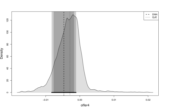
Figure 3: Marginal Effect of Interest Rate

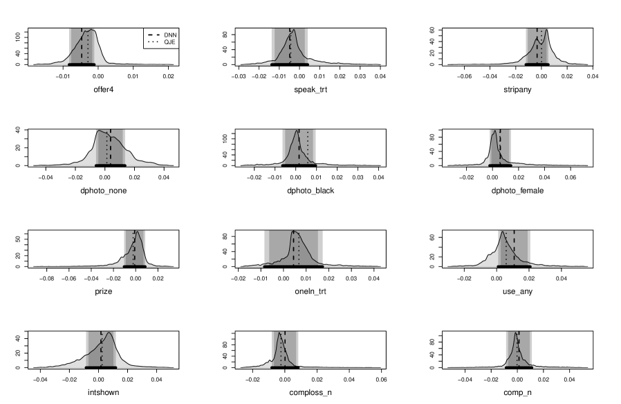
Figure 4: Marginal Effect of Advertising Content

5.3.2 Optimal Personalized Offers

Our framework allows for a rich specification of heterogeneity in the tastes of the consumer. We have shown how standard quantities of interest such as marginal effects can be easily constructed. We now demonstrate how the estimated heterogeneity can be translated into personalized offers and the simplicity with which one can conduct inference on quantities of interest (such as the mean interest rate offered or expected profits).

Given the rarity of defaults, the sample size is too small to uncover full heterogeneity, and therefore we assume that the probably of default given an interest rate $R=r$ is modeled by the function

$$\mathbb{P}[D=1\mid R=r]=D\left(\delta_{0}+\delta_{R}r\right)=\frac{1}{1+\exp\left(-\left[\delta_{0}+\delta_{R}r\right]\right)}.$$

We take these parameters as given. To write the firm’s expected profit for a given consumer, let $L$ be the loan amount and, since we focus on optimizing the interest rate given the parameters, abbreviate $\mathbb{P}[Y=1\mid\bm{X}=\bm{x},\bm{T}=\bm{t}]=G(r)$ and $\mathbb{P}[D=1\mid R=r]=D(r)$. Then

$$\pi(r)=L\big{[}rG(r)\big{]}\big{[}1-D(r)\big{]}.$$ (5.2)

The usual optimization machinery applies and we obtain

$$\frac{\partial\pi(r)}{\partial r}=L\left(r\dot{G}(r)\theta_{R}+G(r)\right)[1-D(r)]-rG(r)\dot{D}(r)\delta_{R}=0,$$

where $\dot{G}$ and $\dot{D}$ represent derivatives with respect to their scalar arguments, as before. Given the structural model, this simplifies to $(r(1-G(r))\theta_{R}+1)-rD(r)\delta_{R}=0$. The optimal interest rate offer, denoted $r^{*}$, is therefore

$$r^{*}=\frac{1+r^{*}(1-G(r^{*}))\theta_{R}}{D(r^{*})\delta_{R}}.$$ (5.3)

This is an implicit function but there will a unique fixed point since the numerator of the right hand side is decreasing in $r$ while denominator is increasing, for $\theta_{R}<0$ and $\delta_{R}>0$. Figure 5 presents a visual representation of Equation (5.3). Each curve corresponds to a distinct consumer profile and the intersection with the $45^{o}$ line represents the fixed point $r^{*}.$ The density then represents the kernel density of the optimal personalized offers $\left(r^{*}\right)$ across consumers. We note that while the fixed points are only shown for a subset of customers (to avoid clutter) the density is computed across the entire sample.

Even though $r^{*}$ is not available in closed form it remains a smooth function of the parameters $\bm{\theta}$, which is all that is required for our method to apply. We can therefore give inference for any statistic of the form (2.2). As a simple example, Figure 5 shows estimation and inference for $\mu_{0}=\mathbb{E}[r^{*}(\bm{\theta}(\bm{x}))]$, i.e. where the function $H$ is the same as the function $r^{*}$. The vertical dashed line is the point estimate, found to be 11.37%, while a 95% confidence interval is shown as the grey region and black segment, founded to be $[9.48\%,13.98\%]$.

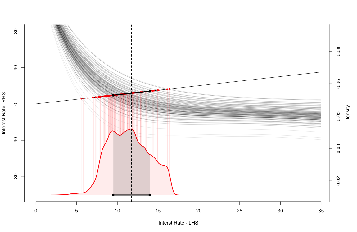
Figure 5: Optimal Personalized Interest Rate Offers

Obtaining confidence intervals for more involved quantities is just as straightforward with our framework. We illustrate by computing the expected profits from setting the optimal personalized interest rate. From (5.2), this is expressed as

$$\mu_{0}=\mathbb{E}\big{[}\pi(r^{*}(\bm{\theta}(\bm{X})))\big{]}=\mathbb{E}\Big{[}L\left[r^{*}(\bm{\theta}(\bm{X}))G(r^{*}(\bm{\theta}(\bm{X})))\right]\left[1-D(r^{*}(\bm{\theta}(\bm{X})))\right]\Big{]}.$$

Then, given the optimal interest rates $r^{*}$, and appealing to the envelope theorem we can obtain the influence function for this quantity ignoring the impact that perturbations in $\bm{\theta}$ have on $r^{*}$ since $\frac{\partial\pi}{\partial r}|_{r=r^{*}}=0$. As such, the influence function for expected profits can be constructed in closed form (conditional on $r^{*})$. Alternatively, one could use standard numerical differentiation or automatic differentiation engines to accomplish the same objective. In our analysis the numerical and exact derivatives give close to identical results. In our analysis we focus on the high risk segment (which is over 75% of the customers) and normalize the loan amount to $L=1$. Since the interest rate is measured in percentage points, we interpret the expected profit construct $\mu_{0}$ as the net average expected income from offering a $100 loan at a personalized interest rate to each potential customer. We find that $\widehat{\mu}_{0}=\$0.3504$ with a 95% confidence interval of $(\$0.1421,\$0.5586)$. Figure 6 depicts the density of profits for each customer along with the estimate and confidence interval of expected profits. The personalized interest rate scheme delivers an incremental 5.7% in expected profits over the optimal (uniform) interest rate derived from the experiment alone. While a more serious application would incorporate a number of additional features into the model and analysis, we feel that our example above suffices as a proof of concept of the value of our approach for applied work.

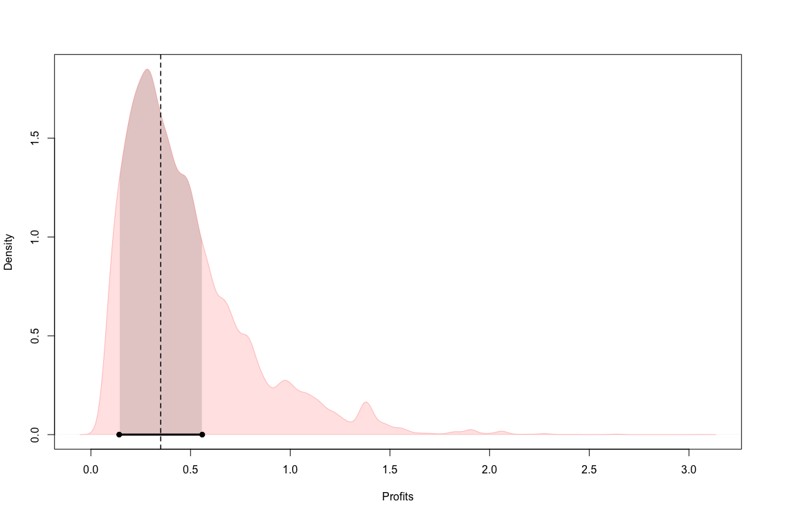
Figure 6: Expected Profits from Personalized Interest Rate Offers

5.4 Summary

This application showcases the simplicity with which parametric models can be extended to incorporate nonparametric heterogeneity via deep neural networks. The structure of the model is maintained which in turn preserves the interpretability of the parameter functions. Since inference in our framework is close to automatic (automatic for data from randomized experiments) it offers the applied researcher a sophisticated yet practical framework for analysis.

6 Examples

Here we discuss several examples that fall within our framework, both to demonstrate the applicability of our results to new and interesting examples as well as to compare to existing results. We emphasize that these examples, and more, are covered without additional derivations: knowing the forms below is useful but not necessary before applying our methodology. This discussion is not exhaustive. We begin with two familiar examples, average treatment effects and partially linear models, before moving on to other cases.

6.1 Average Effect of a Binary Treatment

Average treatment effects are a canonical semiparametric problem and the standard case in the recent literature on inference after machine learning (see references in Section 4.1). Here we have a scalar outcome and $\bm{T}=T=\{0,1\}$ is the scalar binary treatment indicator. The model is (2.3) with $G(u)=u$, so that $\mathbb{E}[Y\mid\bm{x},t]=\theta_{01}(\bm{x})+\theta_{02}(\bm{x})\cdot t$. Letting $Y(t)$ be the potential outcome under treatment $T=t$, we find that $\mathbb{E}[Y(0)\mid\bm{X}=\bm{x}]=\theta_{01}(\bm{x})$ and $\mathbb{E}[Y(1)\mid\bm{X}=\bm{x}]=\theta_{01}(\bm{x})+\theta_{02}(\bm{x})$, so that $\theta_{02}(\bm{x})$ represents the (heterogeneous) conditional average treatment effect, assuming unconfoundedness. Additional mean parameters could be added to cover average treatment effects for specific treatment groups as well as multi-valued treatments. See Cattaneo (2010) and Cattaneo and Farrell (2011) for inference using classical nonparametrics (series) and Farrell (2015) for machine learning (group lasso) results.

The naive approach to estimation would either involve unstructured modeling of $\mathbb{E}[Y\mid\bm{x},t]$ or separate estimation (in the treatment and comparison groups) of $\mathbb{E}[Y(0)\mid\bm{X}=\bm{x}]$ and $\mathbb{E}[Y(1)\mid\bm{X}=\bm{x}]$. Along with the propensity score, these would be inputs into the well-known doubly robust or influence function estimator (Robins et al., 1994; Hahn, 1998). The structured architectures of Figures 1 and 2 intuitively reflect the idea that $\theta_{01}(\bm{x})$ and $\theta_{02}(\bm{x})$ may share similar features, since they relate to the conditional means of the two potential outcomes, under treatment and control. This same notion has been used in the past for trees by Zeileis et al. (2008) and Athey and Imbens (2016), where the treatment and control groups share a partition, and by Farrell et al. (2021) for DNNs, most similar to the present case. Notice that this is different from assuming that the regression functions share similar features to the propensity score, or its inverse, which in general there is no reason to expect to hold, particular in high-dimensional or data-adaptive scenarios. For classical, low-dimensional series estimators, this has been exploited to prove that both regression imputation (Imbens et al., 2007; Cattaneo and Farrell, 2011) and inverse weighting (Hirano et al., 2003) are semiparametrically efficient.

Equation (2.2) gives the familiar average treatment effect by taking $\bm{H}(\bm{x},\bm{\theta};\bm{t}^{*})=\theta_{02}$. In this case, the model (2.1) is without loss of generality beyond unconfoundedness, and hence setting $\ell$ to be squared loss, we recover the familiar efficient influence function. To see this, begin with the univariate form in (4.5), and use the fact that $\dot{H}_{1}=0$, $\dot{H}_{2}=1$, $\lambda_{0}=1$, and $\lambda_{1}(\bm{x})=\lambda_{2}(\bm{x})=\mathbb{P}[T=1|\bm{X}=\bm{x}]:=p(\bm{x})$, the propensity score. Then, adding and subtracting $p(\bm{x})$ and using the fact that $(1-t)t=0$, we have

$$\psi(\bm{w},\bm{\theta},\bm{\Lambda}) =\theta_{02}(\bm{x})+\frac{\dot{H}_{1}(\bm{x})(\lambda_{2}(\bm{x})-\lambda_{1}(\bm{x})t)+\dot{H}_{2}(\bm{x})(\lambda_{0}(\bm{x})t-\lambda_{1}(\bm{x}))}{\lambda_{2}(\bm{x})\lambda_{0}(\bm{x})-\lambda_{1}(\bm{x})^{2}}(y-G(\bm{\theta}(\bm{x})^{\prime}\bm{t}))$$

$$=\theta_{02}(\bm{x})+\frac{(t-p(\bm{x}))(y-\theta_{01}(\bm{x})-\theta_{02}(\bm{x})t)}{p(\bm{x})-p(\bm{x})^{2}}$$

$$=\theta_{02}(\bm{x})+\frac{[(1-p(\bm{x}))t-p(\bm{x})(1-t)](y-\theta_{01}(\bm{x})-\theta_{02}(\bm{x})t))}{p(\bm{x})(1-p(\bm{x}))}$$

$$=\theta_{02}(\bm{x})+\frac{(1-p(\bm{x}))t(y-\theta_{01}(\bm{x})-\theta_{02}(\bm{x})t))}{p(\bm{x})(1-p(\bm{x}))}-\frac{p(\bm{x})(1-t)(y-\theta_{01}(\bm{x})-\theta_{02}(\bm{x})t))}{p(\bm{x})(1-p(\bm{x}))}$$

$$=\theta_{02}(\bm{x})+\frac{t(y-\theta_{01}(\bm{x})-\theta_{02}(\bm{x})t))}{p(\bm{x})}-\frac{(1-t)(y-\theta_{01}(\bm{x})))}{(1-p(\bm{x}))}.$$

In this example, the standard overlap assumption, that the propensity score is bounded away from zero and one, ensures that $\bm{\Lambda}(\bm{x})^{-1}$ is well behaved: the determinant of $\bm{\Lambda}(\bm{x})=p(\bm{x})(1-p(\bm{x}))$, the initial denominator above.

It is straightforward to extend this example in a number of directions. To appreciate how simply and transparently our framework can be applied, suppose that beyond the mean effect, we were interested in the variance of $Y(1)$ versus $Y(0)$. We take a quasi maximum likelihood approach, taking $\ell(\bm{y},\bm{t},\bm{\theta}(\bm{x}))$ to be the Gaussian likelihood, but instead of assuming constant variance (and thus fitting least squares regression) we optimization with respect to two additional parameters by taking the standard deviation to be $\sigma_{1}(\bm{x})t+\sigma_{0}(\bm{x})(1-t)$. The conditions for convexity of the loss are well-known from likelihood theory and can be directly used here.

6.2 Partially Linear Models

A second widely studied semiparametric problem is the partially linear model, where $G(\theta_{01}(\bm{x})+\theta_{02}t)$, that is, where $\theta_{02}$ is assumed constant, and for simplicity we focus on a single scalar treatment variable. Restricting to a constant or homogeneous effect is a strong assumption and should be viewed with caution, but we can still apply our results to this case. Most studies use a linear model, but there are results for nonlinear $G(u)$. For our framework, we set the loss such that $\bm{\ell}_{\bm{\theta}}(\bm{w},\bm{\theta}(\bm{x}))=\bm{t}(G(\bm{\theta}_{0}(\bm{x})^{\prime}\bm{t})-y)$, as discussed above.

Typically, the parameter of interest is $\theta_{02}$, in which case (4.5) gives that $\psi(\bm{w},\bm{\theta},\bm{\Lambda})-\theta_{02}$ is

$$\left[\lambda_{2}(\bm{x})-\frac{\lambda_{1}(\bm{x})^{2}}{\lambda_{0}(\bm{x})}\right]^{-1}\left(t-\frac{\lambda_{1}(\bm{x})}{\lambda_{0}(\bm{x})}\right)\Big{(}y-G(\theta_{01}(\bm{x})+\theta_{02}t)\Big{)}.$$

We must assume that $\lambda_{2}(\bm{x})\lambda_{0}(\bm{x})\neq\lambda_{1}(\bm{x})^{2}$, which for identity $G$ requires positive conditional variance of $T$. In nonlinear models the conditional moments will be weighted by $\dot{G}$ if we have used the appropriate loss. In some cases the nonsingularity will follow from other regularity conditions, such as for the logistic link, where $\dot{G}=G(1-G)$ and the Hessian is invertible under bounded covariates and we use the log-likelihood.

Partially linear models have received a great deal of attention in the literature, most often with a linear link function. Explicitly treating inference following machine learning, the pioneering work of Belloni et al. (2014) proved valid inference after lasso selection. Chernozhukov et al. (2018) use this model as the leading example of their generic results, and present several different Neyman orthogonal scores that could be used. Cattaneo et al. (2018) give novel results for series-based inference with many terms; they also give numerous references that use classical nonparametrics. For the case of nonlinear link function, Carroll et al. (1997) and Mammen and van de Geer (1997) study the nonparametric case, as we do here in Section 3, while Belloni et al. (2016) study high-dimensional sparse models, where $\theta_{01}(\bm{x})=\bm{\theta}_{01}^{\prime}\bm{x}$. Our model is more general, but even so we obtain efficiency in the linear case under homoskedaticity, but not otherwise.

The literature has almost entirely focused on inference on the constant coefficient $\theta_{02}$, but our framework allows for a much richer set of possibilities. For example, in both empirical finance and applied microeconomics the function $\theta_{01}(\bm{x})$ is of interest, see Cattaneo et al. (2020a) and Cattaneo et al. (2019) respectively.

6.3 Continuous Treatments and Average Partial Effects

Moving beyond discrete treatments or homogeneous effects, our framework gives a simple way to assess the heterogeneous effect of a continuous treatment $T$ or set of treatments $\bm{T}$ by recovering average partial effects. In this case we begin with a linear model, $\mathbb{E}[Y\mid\bm{x},\bm{t}]=\theta_{01}+\theta_{02}^{\prime}\bm{t}$, and enrich the slopes and intercept to be parameter functions, so that $\mathbb{E}[Y\mid\bm{x},\bm{t}]=\theta_{01}(\bm{x})+\bm{\theta}_{02}(\bm{x})^{\prime}\bm{t}$.

In this case, a common parameter is the average slope, or slopes, $\bm{\mu}_{0}=\mathbb{E}[\bm{\theta}_{02}(\bm{x})]$. Although we are not restricted to this parameter, it is useful as it is the average of the heterogeneous partial effects, which, thanks to the model, can be extrapolated to any treatment level $\bm{t}^{*}$ by taking $\mathbb{E}[\bm{\theta}_{02}(\bm{x})^{\prime}\bm{t}^{*}]$. Wooldridge (2004) and Graham and Pinto (2018) are the closest to our work in this example, and also give conditions for a causal interpretation of $\mathbb{E}[\theta_{0k}(\bm{X})]$. Hirshberg and Wager (2019) use a different approach to recover the average effect, but briefly discuss double robustness. Chernozhukov et al. (2019) use a similar model with the goal of policy targeting.

Our influence function specializes to exactly the efficient influence function of Graham and Pinto (2018) for $\bm{\mu}_{0}=\mathbb{E}[\bm{\theta}_{02}(\bm{x})]$. Let $\bm{0}_{d}$ be the $d$-long zero vector, $\bm{I}_{d}$ be the $d$-square identity matrix, $\bm{V}(\bm{x})=\mathbb{V}[\bm{T}\mid\bm{x}]$ be the conditional variance, and $\bm{E}(\bm{x})=\mathbb{E}[\bm{T}\mid\bm{x}]$ be the conditional expectation. Then we have $\bm{\Lambda}(\bm{x})=\begin{pmatrix}1&\bm{E}(\bm{x})^{\prime}\\ \bm{E}(\bm{x})&\mathbb{E}[\bm{T}\bm{T}^{\prime}|\bm{x}]\end{pmatrix}$ and $\bm{H}_{\bm{\theta}}=(\bm{0}_{d_{\bm{\mu}}}\;,\;\bm{I}_{d_{\bm{\mu}}})$, so after some algebra, Equation (4.4) gives

$$\bm{\psi}(\bm{w},\bm{\theta},\bm{\Lambda})=\bm{\theta}_{02}(\bm{x})-\bm{V}(\bm{x})^{-1}(\bm{t}-\bm{E}(\bm{x}))(y-\theta_{01}(\bm{x})-\bm{\theta}_{02}(\bm{x})^{\prime}\bm{t}).$$

A simple, but useful extension to the scalar case is when the vector $\bm{T}$ includes polynomials, or other flexible specifications, or interaction terms of several policy variables, and we wish to study heterogeneous effects. That is, for two treatment variables $T_{1}$ and $T_{2}$, we may be interested in the coefficients on $T_{1}^{2}$ or $T_{1}\times T_{2}$. Taking $T_{2}$ to be a binary or categorical variable would yield subgroup effects. Such objects are routinely studied in the parametric case, and here we allow full heterogeneity in these effects, beyond the original treatment or partial effect.

The example of average partial effects, when combined with transformations of the outcome and the treatment, recovers many other useful settings, even restricting to linear link functions. To give just two examples, consider the so-called Berry logit and Cobb-Doublas production. The former, pioneered by Berry (1994), is a popular model for demand models where the outcome of interest is the market share distribution across firms. In most applications the researcher has access to outcomes $\{Y_{jm}\}$ which represent a collection of $j=0\dots J$ market shares across $m=1\dots M$ markets. The objective is then to model these as a function of firm (marketing) decisions $\bm{t}_{jm}$ (see e.g. Nevo (2001)). We can introduce heterogeneity across markets by allowing for the marketing effects to be moderated by consumer characteristics $\bm{x}_{m}$, so that we can write a collection of $(J-1)$ equations as follows

$$\mathbb{E}\left[\left.\log\frac{Y_{jm}}{Y_{0m}}\right|\bm{X}=\bm{x}_{m},\bm{T}_{jm}=\bm{t}_{jm}\right]=\theta_{01j}(\bm{x}_{m})+\bm{\theta}_{02}(\bm{x}_{m})^{\prime}(\bm{t}_{jm}-\bm{t}_{0m}).$$

Stacking these equations and the corresponding data allows us to construct an estimator for $\theta_{01j}(\bm{x}_{m})$ and $\bm{\theta}_{02}(\bm{x}_{m})$. We note here that our framework can be extended to include instruments along the lines of Okui et al. (2012).

The Cobb-Douglas specification for production functions is denoted by $Y=CK^{\theta_{01}(\bm{x})}L^{\theta_{02}(\bm{x})}$. With $\bm{T}=(K,L)^{\prime}$, by taking logs we can write this model in our format, as

$$\mathbb{E}\left[\log{Y}\mid\bm{X}=\bm{x},K=k,L=l\right]=\log C+\theta_{01}(\bm{x})\cdot\log k+\theta_{02}(\bm{x})\cdot\log l.$$

Given estimates we may be interested in understanding if the technology exhibits increasing, constant, or decreasing returns to scale. This can be ascertained by computing $\bm{\mu}_{0}=\mathbb{E}[\theta_{01}(\bm{x})+\theta_{02}(\bm{x})]$ and noting that $\bm{\mu}_{0}<1,\bm{\mu}_{0}=1,\bm{\mu}_{0}>1$ imply decreasing, constant, and increasing returns to scale. The Cobb-Douglas specification has also been used in demand settings and marketing mix models and the framework described above would be readily applicable there as well.

It is useful to contrast our model, $\mathbb{E}[Y\mid\bm{x},\bm{t}]=\theta_{01}(\bm{x})+\bm{\theta}_{02}(\bm{x})^{\prime}\bm{t}$, with the fully unrestricted case, $\mathbb{E}[Y\mid\bm{x},\bm{t}]=\theta_{0}(\bm{x},\bm{t})$. For causal inference in particular, this case has been studied by Hirano and Imbens (2004) and, using doubly robust approaches, Kennedy et al. (2017) and Colangelo and Lee (2020). The unrestricted model may increase the generality of the results but can make inference and interpretation more difficult. Here our model imposes nontrivial structure, unlike in the binary case, but yields a tractable and interpretable model. From a practical point of view, compared to $\mathbb{E}[Y\mid\bm{x},\bm{t}]=\theta_{0}(\bm{x},\bm{t})$, our approach results in lower dimensional estimation and does not require conditional density estimation, which can be challenging in high dimensional, complex settings.

Another related area is the study of (weighted) average derivatives, a common estimand in the literature on semiparametric theory (Powell et al., 1989; Newey and Stoker, 1993). Here the object of interest is $\mathbb{E}[w(\bm{x},\bm{t})\partial\theta(\bm{x},\bm{t})/\partial\bm{t}]$ for a known weighting function $w(\bm{x},\bm{t})$. This represents the average of a linear approximation of an unstructured relationship of $\bm{T}$ to $Y$. Our approach is perhaps more direct and transparent: if a linear approximation is of interest in the end, we directly enrich the linear approximation, rather than recover it from a more complex object.

6.4 Fractional Outcomes

Building on the previous example, we emphasize that nonlinear models be covered seamlessly, given appropriate regularity. One widely-used case is fractional outcome models, following Papke and Wooldridge (1996). In these models the outcome $Y$ is continuous but restricted to lie in $[0,1]$. In that paper, the sampling units are firms and $Y$ is the rate of employee partitioning in 401(k) plans. The policy variable is the employer match rates. Papke and Wooldridge (1996) apply a parametric logitistic QLME, explicitly advocating the use of structure to ensure that the outcomes remain on the unit interval. They argue that this specification is valid even at the endpoints and is more practically relevant then transformations of the dependent variable.

We take their model and enrich it to allow for heterogeneity. In our notation, Papke and Wooldridge (1996) assume $\mathbb{E}[Y\mid\bm{X}=\bm{x},T=t]=G(\theta_{01}+\theta_{02}\cdot t+\bm{\gamma}^{\prime}\bm{x})$, with $G$ the logistic link; a structured, but rigid, parametric model with the covariates. We allow for the much more general $\mathbb{E}[Y\mid\bm{X}=\bm{x},T=t]=G(\theta_{01}(\bm{x})+\theta_{02}(\bm{x})\cdot t)$.

The substantive quantities of interest in the original application is the marginal effect of the match rate on participation and the degree to which this marginal effect exhibits diminishing patterns. To investigate this Papke and Wooldridge (1996) evaluate the marginal effect at fixed values of $\mathbf{x}$ and several match rates, $t^{*}\in\left\{0.0,0.5,1.0\right\}$. They conclude that there exists evidence for diminishing marginal effects, for example.

We can generalize these findings by conducting inference on the average marginal effect (AME) and the average change in the marginal effect (ACME), given by

$$\text{AME}\left(t^{*}\right)=\mathbb{E}\left[\left.\frac{\partial\mathbb{E}[Y\mid\mathbf{X},t]}{\partial t}\right|_{t=t^{*}}\right]\quad\text{ and }\quad\text{ACME}\left(t^{*}\right)=\mathbb{E}\left[\left.\frac{\partial^{2}\mathbb{E}[Y\mid\mathbf{X},t]}{\partial t^{2}}\right|_{t=t^{*}}\right].$$

Because of the structure of the model, these are easily recovered in the form of $\bm{\mu}_{0}$, by taking $H_{\text{AME}}\left(\bm{x},\bm{\theta};t^{*}\right)=\theta_{02}G^{*}\left(1-G^{*}\right)$ and $H_{\text{ACME}}\left(\bm{x},\bm{\theta};t^{*}\right)=\theta_{02}^{2}G^{*}\left(1-G^{*}\right)\left(1-2G^{*}\right)$, respectively, where $G^{*}=G(\bm{\theta}^{\prime}\bm{t}^{*})$. Note the contrast with the naive, unstructured ML approach, where recovering the second derivative of a complex, high-dimensional $G(\hat{u}(\bm{x},t))$ could be challenging.

Our deep neural networks can be structured to respect fractional losses by using the QMLE logistic loss as the model (2.1) while assuming the mean restriction (2.3). For estimation and inference, we must assume that $\mathbb{E}[\dot{G}\bm{T}\bm{T}^{\prime}|\bm{x}]$ is nonsingular, again a weighted conditional variance assumption. Theorem 2 (or in this case, Equations (4.4) or (4.5)) apply immediately. The derivatives required for $\ell$ are well known from likelihood theory and can be used directly. Those for $H$ are easily available or can be computed if necessary.

6.5 Type I Tobit

To illustrate the use of existing likelihood theory for parametric models and how these can help interpret our requirements, consider the type I Tobit model. This is a case where our assumptions are conditional versions of the standard conditions required for parametric MLE and therefore we can intuitively understand our conditions by imagining our method as if it was parametric MLE for each value $\bm{x}$.

Here we assume that the observed outcome is $Y=\max(0,Y^{*})$, where $Y^{*}$ is Gaussian given $\bm{x}$ with mean given by, say $\bm{\beta}_{0}(\bm{x})^{\prime}\bm{t}$ and variance $\sigma^{2}(\bm{x})$ (in practice one may take $\sigma^{2}(\bm{x})=\exp\{\tilde{\sigma}(\bm{x})\}$ for example). In this case, we work with the transformed parameters $\bm{\theta}(\bm{x})=(\bm{\theta}_{1}(\bm{x})^{\prime},\theta_{2}(\bm{x}))^{\prime}$, with $\bm{\theta}_{1}(\bm{x})=\bm{\beta}_{0}(\bm{x})/\sigma(\bm{x})$ and $\theta_{2}(\bm{x})=\sigma^{-1}(\bm{x})$. See Amemiya (1985) and Wooldridge (2010) for textbook treatments and details on the calculations below.

The gradient and Hessian are cumbersome but known. These can be used both for understanding the assumptions required but also, if desired, in the computation. Let $\mathbbm{1}_{0}=\mathbbm{1}\{Y^{*}\leq 0\}$ and $\mathbbm{1}_{1}=\mathbbm{1}\{Y^{*}>0\}$. Let $\phi$ and $\Phi$ denote the Gaussian density and distribution functions. Then the gradient (score) terms are

$$\bm{\ell}_{\bm{\theta}_{1}}(\bm{w},\bm{\theta}(\bm{x}))=\mathbbm{1}_{0}\frac{\phi(\bm{\theta}_{1}(\bm{x})^{\prime}\bm{t})\bm{t}}{1-\Phi(\bm{\theta}_{1}(\bm{x})^{\prime}\bm{t})}-\mathbbm{1}_{1}\Big{(}\theta_{2}(\bm{x})y-\bm{\theta}_{1}(\bm{x})^{\prime}\bm{t}\Big{)}\bm{t}^{\prime}$$

and

$$\bm{\ell}_{\theta_{2}}(\bm{w},\bm{\theta}(\bm{x}))=-\mathbbm{1}_{1}\theta_{2}(\bm{x})^{-1}+\mathbbm{1}_{1}(\theta_{2}(\bm{x})y-\bm{\theta}_{1}(\bm{x})^{\prime}\bm{t})y.$$

The second derivatives are

$$\bm{\ell}_{\bm{\theta}_{1}\bm{\theta}_{1}}(\bm{w},\bm{\theta}(\bm{x}))=-\mathbbm{1}_{0}\frac{\phi(\bm{\theta}_{1}(\bm{x})^{\prime}\bm{t})(\bm{\theta}_{1}(\bm{x})^{\prime}\bm{t})\bm{t}\bm{t}^{\prime}}{1-\Phi(\bm{\theta}_{1}(\bm{x})^{\prime}\bm{t})}+\mathbbm{1}_{0}\frac{\phi(\bm{\theta}_{1}(\bm{x})^{\prime}\bm{t})^{2}\bm{t}\bm{t}^{\prime}}{[1-\Phi(\bm{\theta}_{1}(\bm{x})^{\prime}\bm{t})]^{2}}+\mathbbm{1}_{1}\bm{t}\bm{t}^{\prime},$$

$$\ell_{\theta_{2}\theta_{2}}(\bm{w},\bm{\theta}(\bm{x}))=-\mathbbm{1}_{1}\theta_{2}(\bm{x})^{-2}+\mathbbm{1}_{1}y^{2},\qquad\text{ and }\qquad\bm{\ell}_{\theta_{1}\theta_{2}}(\bm{w},\bm{\theta}(\bm{x}))=\mathbbm{1}_{1}y\bm{t}.$$

That the gradients are conditionally mean zero can be directly verified. The matrix $\bm{\Lambda}(\bm{x})^{-1}$ exists because $\bm{\theta}_{1}(\bm{x})^{\prime}\bm{t}-\phi(\bm{\theta}_{1}(\bm{x})^{\prime}\bm{t})/[1-\Phi(\bm{\theta}_{1}(\bm{x})^{\prime}\bm{t})]>0$, using exactly the logic from parametric models (Donald, 1990; Olsen, 1978; Amemiya, 1985). Naturally other conditions, such as smoothness, would be required for the functions $\bm{\beta}(\bm{x})$ and $\sigma(\bm{x})$ and would need to be matched by the neural network, or other nonparametric estimator.

6.6 Multinomial Choice

The binary choice model examined in the application naturally extends to multiple choices. Here the model (2.1) deals with a vector of outcomes. Let there be $J\geq 1$ choices, in addition to the outside option. The outcome is the categorical variable $Y\in\{0,1,\ldots,J\}$ or the vector $\bm{Y}=(Y_{1},Y_{2},\ldots,Y_{J})^{\prime}$, with $Y_{j}=\mathbbm{1}\{Y=j\}$. The standard assumption is that

$$\mathbb{P}[Y=j\mid\bm{X}=\bm{x},\bm{T}=\bm{t}]=G_{j}\left(u_{1},u_{2},\ldots,u_{J}\right),\quad\text{ with }\quad G_{j}=\frac{\exp\{u_{j}\}}{1+\sum_{m=1}^{J}\exp\{u_{m}\}},$$

for utility functions $u_{j}=u_{j}(\bm{x},\bm{t})$, with $u_{0}$ normalized to zero. If we let $G_{j}=G_{j}(u_{0},u_{1},\ldots,u_{J})$, then using that $Y_{0}+Y_{1}+\cdots+Y_{J}=1$, $u_{0}=0$, and the form of $G_{j}$, the log-likelihood is

$$\ell=\log(G_{0})+\sum_{j=1}^{J}y_{j}u_{j}.$$

The negative would be the loss we minimize.

The specification of the utility functions gives rise to different parametric models in this context. The defacto standard in many disciplines is McFadden’s multinomial choice model, and our enriched version would assume that the utilities obey

$$u_{j}(\bm{x},\bm{t}_{j})=\theta_{01j}(\bm{x})+\bm{\theta}_{02}(\bm{x})^{\prime}\bm{t}_{j},\quad j=1,\ldots,J,$$

where the $\bm{t}_{j}$ are option-specific characteristics, such as prices. The key restriction is that, while the intercept functions are choice-specific, the price effect functions are common across options. This model is well studied, and the gradient $\bm{\ell}_{\bm{\theta}}(\bm{w},\bm{\theta}(\bm{x}))$ and Hessian $\bm{\ell}_{\bm{\theta}\bm{\theta}}(\bm{w},\bm{\theta}(\bm{x}))$ are well understood. The parameter $\bm{\mu}_{0}$ could depend on any of the intercept and slope functions. The orthogonal score can then be read off from Theorem 2. The result is completely new to the literature and, as above, fully implementable.

6.7 Instrumental Variables

For linear models, such as in Section 6.1 or 6.3, a natural extension is to endogenous variables of interest. Consider for simplicity the case with a single endogenous treatment variable and a single instrument $Z$. It is natural in our setting to allow fully flexible observed heterogeneity in the effects of the instrument. We therefore arrive at the two-equation model

$$Y =\theta_{01}(\bm{X})+\theta_{02}(\bm{X})T+V,$$ (6.1)

$$T =\zeta_{01}(\bm{X})+\zeta_{02}(\bm{X})Z+U,$$ (6.2)

where $\mathbb{E}[V\mid\bm{X},Z]=\mathbb{E}[U\mid\bm{X},Z]=0$. For estimation, and moreover, derivation of an orthogonal score, we simply plug (6.2) into (6.1) to obtain the reduced form equation

$$\begin{split}&Y=\alpha_{0}(\bm{X})+\beta_{0}(\bm{X})Z+\tilde{V},\\ &\alpha_{0}(\bm{x})=\theta_{01}(\bm{x})+\theta_{02}(\bm{x})\zeta_{01}(\bm{x}),\quad\beta_{0}(\bm{x})=\theta_{02}(\bm{x})\zeta_{02}(\bm{x}),\quad\tilde{V}=\theta_{02}(\bm{X})U+V.\end{split}$$ (6.3)

Using the instruments in this way directly generalizes the standard two stage least squares approach to handle high-dimensional, complex observed heterogeneity. Deep learning is again well-suited to estimating the coefficient functions in (6.2) and (LABEL:eqn:iv_reduced_form), exactly following Section 3. The loss (2.1) is simply the sum of the two squared losses.

With this notation, we aim to recover a parameter that depends on the coefficient functions of (6.2) and (LABEL:eqn:iv_reduced_form), given by

$$\bm{\mu}_{0}=\mathbb{E}\left[H\left(\bm{X},\alpha_{0},\beta_{0},\zeta_{01},\zeta_{02};\bm{t}^{*}\right)\right].$$ (6.4)

The leading case is the average partial effect of the endogenous variable $T$: $\bm{\mu}_{0}=\mathbb{E}[\theta_{02}(\bm{X})]=\mathbb{E}[\beta_{0}(\bm{X})/\zeta_{02}(\bm{X})]$. Note that here we are assuming the analogue of strong instruments, as we need $\zeta_{02}(\bm{X})$ to be nowhere zero.

To show the score in this case, define $\bm{\theta}=(\alpha_{0},\beta_{0},\zeta_{01},\zeta_{02})^{\prime}$, $\bm{w}=(y,t,z)$, $\bm{t}=(1,t)^{\prime}$, $\bm{z}=(1,z)^{\prime}$ and $\bm{I}_{2}$ the $2\times 2$ identity. Then we have

$$\bm{\ell}_{\bm{\theta}}(\bm{w},\bm{\theta}(\bm{x}))=-\begin{pmatrix}y-\alpha_{0}(\bm{x})-\beta_{0}(\bm{x})z\\ t-\zeta_{01}(\bm{x})-\zeta_{02}(\bm{x})z\end{pmatrix}\otimes\bm{z}\quad\text{and }\quad\bm{\ell}_{\bm{\theta}\bm{\theta}}(\bm{w},\bm{\theta}(\bm{x}))=\bm{I}_{2}\otimes\bm{z}\bm{z}^{\prime}.$$

Therefore $\bm{\Lambda}(\bm{x})=\bm{I}_{2}\otimes\bm{\Lambda}_{Z}(\bm{x})$, where $\bm{\Lambda}_{Z}(\bm{x})=\mathbb{E}[\bm{z}\bm{z}^{\prime}\mid\bm{X}=\bm{x}]$. These can be inserted directly into Equation (4.3).

This approach is far from the only option in instrumental variable models. Indeed, for the special case of homogeneous effects in a partially linear IV model, Chernozhukov et al. (2018) study two different scores, Equations (4.7) and (4.8) therein, and also mention in footnote 8 that their stated method for constructing orthogonal scores would yield a third option. Different scores sometimes require that different functions be estimated in the first step or as part of the correction term. Our approach here aims for ease of use and transparency: (6.2) and (LABEL:eqn:iv_reduced_form) can be directly estimated using the deep learning architectures of Section 3.

7 Extensions

Our framework is connected to many different areas of debiasing for inference, some of which have been explored in settings we have ruled out. Our methodological ideas could be extended to many of these settings.

Building on our two-step approach, we could consider more general two-step GMM type problems, where the first step has been enriched with deep learning. In some cases, our results can be extended directly, at mainly a notational cost. For example, $\bm{\mu}_{0}$ need not be restricted to a closed form, but could defined in terms of an objective function or moment condition itself. That is, (2.2) could be changed such that $\bm{\mu}_{0}$ solved $\max_{\bm{\mu}}\mathbb{E}[\bm{H}(\bm{X},\bm{\mu},\bm{\theta}_{0}(\bm{X});\bm{t}^{*})]$ or $\mathbb{E}[\bm{H}(\bm{X},\bm{\mu},\bm{\theta}_{0}(\bm{X});\bm{t}^{*})]=0$. In other cases, more substantial work would be necessary. Extending our ideas to quantile regression and other nonsmooth objective functions would be such an example. The extent to which general, easily implementable results can be given in such cases is an interesting avenue for future research.

An important point of our framework is that the parameter functions $\bm{\theta}(\bm{x})$ have economic meaning and interpretability. A useful extension to this would be to consider shape restrictions; see Chetverikov et al. (2018) for review. For example, price coefficients should be nonpositive, and $\theta<0$ is often found or enforced in parametric modeling. In our context, we would like to ensure that $\theta(\bm{x})<0$. In our experience, the discipline of the model often yields functions which empirically obey such restrictions, i.e., loosely speaking, the model regularizes the data toward economically-valid estimates. However, this does not always hold, and it would be interested to enforce this during the estimation and establish second-step inference. One possibility to enforce such shape constraints is by designing a proper barrier function added to the original loss, thus to leverage techniques developed in constrained optimization (Nesterov and Nemirovskii, 1994). Provided the approximation results still hold, a version of Theorem 1 could be obtained, after which inference using the influence function can proceed.

Another important extension for some applications would be to consider the case when the number of variables of interest is large. In this case, our ideas connect with the literature on debiasing in high dimensional regression. Consider the case of a conditional mean restriction with a linear function, so that $\mathbb{E}[Y\mid\bm{x},\bm{t}]=\bm{\theta}_{0}(\bm{x})^{\prime}\bm{t}$. A fundamental tension exists between the dimensionality of $\bm{T}$ and the complexity allowed for in $\bm{\theta}_{0}(\bm{X})$. We have studied the case of fully flexible heteregeneity for a low-dimensional $\bm{T}$. When $\bm{T}$ is high dimensional, estimation of these functions will not be possible, at least not with sufficient precision to allow for inference. There is thus a natural tradeoff between the dimensionality of the treatment variables and the complexity of the heterogeneity. If a researcher can a priori restrict the form of the heterogeneity such that the functions $\bm{\theta}_{0}(\bm{x})$ are simple, or in the extreme case, constant, then useful results can be obtained. For this model, Javanmard and Montanari (2018) seek a Gaussian limit for $\sqrt{n}(\bm{\widehat{\theta}}-\bm{\theta}_{0})$ where

$$\bm{\widehat{\theta}}=\bm{\widehat{\theta}}_{\text{lasso}}+\frac{1}{n}\widehat{\bm{\Lambda}}\bm{T}_{n}\left(\bm{Y}_{n}-\bm{T}_{n}\bm{\widehat{\theta}}_{\text{lasso}}\right),$$

where $\bm{\widehat{\theta}}_{\text{lasso}}$ is the lasso estimator and $\widehat{\bm{\Lambda}}$ is an estimator of $\bm{\Lambda}=\mathbb{E}[\bm{T}\bm{T}^{\prime}]$, which is not a function of $\bm{X}$ in this restricted model, and the data is $\bm{Y}_{n}=(y_{1},\ldots,y_{n})$ and $\bm{T}_{n}=(\bm{t}_{1}^{\prime},\ldots,\bm{t}_{n}^{\prime})^{\prime}$. The above display is in perfect analogy with our Theorem 2 (in particular, the form in Corollary 2), and the second term serves essentially the same function in both cases. One may check that perturbations to $\bm{\theta}$ do not have a first order impact in expectation, as required for Neyman orthogonality. Similar to our Theorem 3, they require that $\bm{\widehat{\theta}}_{\text{lasso}}$ and $\widehat{\bm{\Lambda}}$ are “good enough” first-stage estimators of $\bm{\theta}_{0}$ and $\bm{\Lambda}$, respectively, which they prove for sparse regression under conditions on the design $\bm{T}_{n}$.

The linear model above rules out all heterogeneity, and is therefore less interesting for our present purpose. An open question is how much flexible heterogeneity can be accommodated which still obtaining useful results. Moving slightly beyond constant effects, Kozbur (2020) allows for a flexible intercept, so that $\mathbb{E}[Y\mid\bm{X}=\bm{x},\bm{T}=\bm{t}]=\theta_{01}(\bm{x})+\bm{\theta}_{02}^{\prime}\bm{t}$, and studies inference on functionals. Our ideas can be adapted to this model. The architecture we proposed in Section 3, shown in Figure 2, will need adjustment. Instead of learning the functions in the parameter layer, the model layer will learn weights for edge between $\bm{t}$ and the outcome. Some form of regularization will be needed in this layer, and thus the end result will be a combination of deep learning and regularized high dimensional regression. A formal exploration of this is a promising direction for future research.

8 Conclusion

We have provided a complete methodological framework for using machine learning to enrich economic models to exploit rich, complex data on individual heterogeneity. We showed that deep learning is ideally suited to this task among modern machine learning methods and we detailed a new network architecture that is designed to estimate economically meaningful objects, moving past pure prediction and towards structural modeling. We gave results for the estimation of heterogeneity using deep learning, showing how our architecture delivers improved rates of convergence. Subsequent inference is proven valid building on a newly calculated influence function with broad applicability.

Our framework covers a wide variety of interesting contexts. The combination of the specification we adopt, the availability of computing infrastructure, and the theory presented above offer a perfect package for applied researchers.

9 References

Appendix A Proofs for Deep Learning

We now prove results stated in the main text for deep learning. First, we show that $\bm{\theta}_{0}(\bm{x})$ is identified and then we prove the rates of convergence for these functions. Lastly we discuss estimation of $\bm{\Lambda}(\bm{x})$.

A.1 Proof of Theorem 1

The proof method of Farrell et al. (2021) is used here. Some details will be deferred to that paper.

Let $M$ be such that $\max_{k\leq d_{\bm{\theta}}}\|\theta_{0k}\|_{\infty}<M$ and functions computed by $\mathcal{F}_{\rm DNN}$ are similarly bounded by $2M$. Define $\bm{\theta}_{n}\in\mathcal{F}_{\rm DNN}$ as the best approximation to $\bm{\theta}_{0}$ in the class of DNNs and let $\epsilon_{n}$ denote the error of the approximation:

$$\bm{\theta}_{n}=\operatorname*{arg\,min}_{\begin{subarray}{c}\bm{\theta}\in\mathcal{F}_{\rm DNN}\\ \|\bm{\theta}\|_{\infty}\leq 2M\end{subarray}}\|\bm{\theta}-\bm{\theta}_{0}\|_{\infty},\qquad\qquad\epsilon_{n}=\|\bm{\theta}_{n}-\bm{\theta}_{0}\|_{\infty}.$$

Under Assumption 2 this error is controlled by the width and depth of an MLP, and we specify to this case at the end of the proof. Here we allow for other approximation assumptions (such as other smoothness classes) and other architectures by leaving the approximation generic.

By Assumption 1 and that $\bm{\widehat{\theta}}$ optimizes $\ell$ over $\mathcal{F}_{\rm DNN}$ in the data,

$$c_{1}\mathbb{E} \left[\|\bm{\widehat{\theta}}(\bm{X})-\bm{\theta}_{0}(\bm{X})\|_{2}^{2}\right]$$

$$\leq\mathbb{E}[\ell(\bm{Y},\bm{T},\bm{\widehat{\theta}}(\bm{X}))]-\mathbb{E}[\ell(\bm{Y},\bm{T},\bm{\theta}_{0}(\bm{X}))]$$

$$\leq\mathbb{E}[\ell(\bm{Y},\bm{T},\bm{\widehat{\theta}}(\bm{X}))]-\mathbb{E}[\ell(\bm{Y},\bm{T},\bm{\theta}_{0}(\bm{X}))]-\mathbb{E}_{n}[\ell(\bm{Y},\bm{T},\bm{\widehat{\theta}}(\bm{X}))]+\mathbb{E}_{n}[\ell(\bm{Y},\bm{T},\bm{\theta}_{n}(\bm{X}))]$$

$$=\left(\mathbb{E}-\mathbb{E}_{n}\right)\left[\ell(\bm{Y},\bm{T},\bm{\widehat{\theta}}(\bm{X}))-\ell(\bm{Y},\bm{T},\bm{\theta}_{0}(\bm{X}))\right]+\mathbb{E}_{n}\left[\ell(\bm{Y},\bm{T},\bm{\theta}_{n}(\bm{X}))-\ell(\bm{Y},\bm{T},\bm{\theta}_{0}(\bm{X}))\right].$$

Applying Farrell et al. (2021, (A.2)) to the second term of the last line above, we find that with probability $1-e^{-\gamma}$

$$c_{1}\mathbb{E}\left[\|\bm{\widehat{\theta}}(\bm{X})-\bm{\theta}_{0}(\bm{X})\|_{2}^{2}\right]\\ \leq\left(\mathbb{E}-\mathbb{E}_{n}\right)\left[\ell(\bm{Y},\bm{T},\bm{\widehat{\theta}}(\bm{X}))-\ell(\bm{Y},\bm{T},\bm{\theta}_{0}(\bm{X}))\right]+c_{2}\epsilon_{n}^{2}+\epsilon_{n}\sqrt{\frac{2C_{\ell}^{2}\gamma}{n}}+\frac{7C_{\ell}M\gamma}{n}.$$ (A.1)

We now apply the localization-based analysis of Farrell et al. (2021) to the first term above and then collect the results. Suppose that for some $r_{0}$, $\mathbb{E}[\|\bm{\widehat{\theta}}(\bm{X})-\bm{\theta}_{0}(\bm{X})\|_{2}^{2}]^{1/2}\leq r_{0}$, which can always be attained given the boundedness. Let $\mathcal{F}^{0}_{\rm DNN}$ be the subset of $\mathcal{F}_{\rm DNN}$ such that $\bm{\theta}\in\mathcal{F}^{0}_{\rm DNN}$ if $\mathbb{E}[\|\bm{\theta}(\bm{X})-\bm{\theta}_{0}(\bm{X})\|_{2}^{2}]^{1/2}\leq r_{0}$. Then by Theorem 2.1 in Bartlett et al. (2005), for $\mathcal{G}=\{g=\ell(\bm{y},\bm{t},\bm{\theta}(\bm{x}))-\ell(\bm{y},\bm{t},\bm{\theta}_{0}(\bm{x})):\bm{\theta}\in\mathcal{F}^{0}_{\rm DNN}\}$, we find that, with probability at least $1-2e^{-\gamma}$, the empirical process term of (A.1) is bounded as

$$\left(\mathbb{E}-\mathbb{E}_{n}\right)\left[\ell(\bm{Y},\bm{T},\bm{\widehat{\theta}}(\bm{X}))-\ell(\bm{Y},\bm{T},\bm{\theta}_{0}(\bm{X}))\right]\leq 6\mathbb{E}_{\eta}R_{n}\mathcal{G}+\sqrt{\frac{2C_{\ell}^{2}r_{0}^{2}\gamma}{n}}+\frac{23\cdot 3MC_{\ell}}{3}\frac{\gamma}{n},$$ (A.2)

where

$$R_{n}\mathcal{G}=\sup_{g\in\mathcal{G}}\frac{1}{n}\sum_{i=1}^{n}\eta_{i}g(\bm{w}_{i})=\sup_{\bm{\theta}\in\mathcal{F}^{0}_{\rm DNN}}\frac{1}{n}\sum_{i=1}^{n}\eta_{i}\left(\ell(\bm{y},\bm{t},\bm{\theta}(\bm{x}))-\ell(\bm{y},\bm{t},\bm{\theta}_{0}(\bm{x}))\right).$$

is the empirical Rademacher complexity and $\mathbb{E}_{\eta}R_{n}\mathcal{G}$ is its expectation holding fixed the data, i.e. over the i.i.d. Rademacher variables $\eta_{i}$. The argument given in Section A.2.2 of Farrell et al. (2021) does not apply directly to $\mathbb{E}_{\eta}R_{n}\mathcal{G}$ because $\bm{\theta}$ is vector valued. Instead, we replace Lemma 2 therein with (Maurer, 2016, Corollary 1), which in our context yields (below $\eta_{ik}$’s denote i.i.d. Rademacher random variables)

$$\mathbb{E}_{\eta}\sup_{\bm{\theta}\in\mathcal{F}^{0}_{\rm DNN}}\frac{1}{n}\sum_{i=1}^{n}\eta_{i}\left(\ell(\bm{y},\bm{t},\bm{\theta}(\bm{x}))-\ell(\bm{y},\bm{t},\bm{\theta}_{0}(\bm{x}))\right) \leq\sqrt{2}C_{\ell}\mathbb{E}_{\eta}\sup_{\bm{\theta}\in\mathcal{F}^{0}_{\rm DNN}}\sum_{k=1}^{d_{\bm{\theta}}}\frac{1}{n}\sum_{i=1}^{n}\eta_{ik}\big{(}\theta_{k}(\bm{x}_{i})-\theta_{0k}(\bm{x}_{i})\big{)}$$

$$\leq\sqrt{2}C_{\ell}\sum_{k=1}^{d_{\bm{\theta}}}\mathbb{E}_{\eta}\sup_{\theta_{k}\in\mathcal{F}^{0}_{\rm DNN,k}}\frac{1}{n}\sum_{i=1}^{n}\eta_{ik}\big{(}\theta_{k}(\bm{x}_{i})-\theta_{0k}(\bm{x}_{i})\big{)},$$

with the second inequality following because the class of DNNs $\mathcal{F}_{\rm DNN}$ we use is decomposable with respect to each coordinate, and therefore we can bound one coordinate at a time.

We then apply Section A.2.1 and Lemmas 3 and 4 of Farrell et al. (2021) to the term for each component function $\theta_{k}$, $k=1,\ldots,d_{\bm{\theta}}$, yielding

$$\mathbb{E}_{\eta}\sup_{\theta_{k}\in\mathcal{F}^{0}_{\rm DNN,k}}\frac{1}{n}\sum_{i=1}^{n}\eta_{ik}\big{(}\theta_{k}(\bm{x}_{i})-\theta_{0k}(\bm{x}_{i})\big{)}\leq 32r_{0}\sqrt{\frac{{\rm Pdim}(\mathcal{F}_{\rm DNN,k})}{n}\left(\log\frac{2eM}{r_{0}}+\frac{3}{2}\log n\right)},$$

with probability $1-\exp^{-\gamma}$, where ${\rm Pdim}(\mathcal{F})$ is the pseudo-dimension of the class $\mathcal{F}$. Therefore, whenever $r_{0}\geq 1/n$ and $n\geq(2eM)^{2}$,

$$\mathbb{E}_{\eta}\sup_{\bm{\theta}\in\mathcal{F}^{0}_{\rm DNN}}\frac{1}{n}\sum_{i=1}^{n}\eta_{i}\left(\ell(\bm{y},\bm{t},\bm{\theta}(\bm{x}))-\ell(\bm{y},\bm{t},\bm{\theta}_{0}(\bm{x}))\right)\leq Kr_{0}\sqrt{\frac{{\rm Pdim}(\mathcal{F}_{\rm DNN})}{n}\log n},$$

for a constant $K$ that depends on $C_{\ell}$ and $d_{\bm{\theta}}$.

This last bound is then combined with (A.2) and put into (A.1) and we find that

$$c_{1} \mathbb{E}\left[\|\bm{\widehat{\theta}}(\bm{X})-\bm{\theta}_{0}(\bm{X})\|_{2}^{2}\right]$$

$$\leq 6Kr_{0}\sqrt{\frac{{\rm Pdim}(\mathcal{F}_{\rm DNN})}{n}\log n}+\sqrt{\frac{2C_{\ell}^{2}r_{0}^{2}\gamma}{n}}+\frac{23\cdot 3MC_{\ell}}{3}\frac{\gamma}{n}+c_{2}\epsilon_{n}^{2}+\epsilon_{n}\sqrt{\frac{2C_{\ell}^{2}\gamma}{n}}+\frac{7C_{\ell}M\gamma}{n}$$

$$\leq r_{0}\left(6K\sqrt{\frac{{\rm Pdim}(\mathcal{F}_{\rm DNN})}{n}\log n}+\sqrt{\frac{2C_{\ell}^{2}\gamma}{n}}\right)+c_{2}\epsilon_{n}^{2}+\epsilon_{n}\sqrt{\frac{2C_{\ell}^{2}\gamma}{n}}+K_{2}\frac{\gamma}{n}$$

$$\leq r_{0}\left(K_{1}\sqrt{\frac{WL\log(W)}{n}\log n}+\sqrt{\frac{2C_{\ell}^{2}\gamma}{n}}\right)+c_{2}\epsilon_{n}^{2}+\epsilon_{n}\sqrt{\frac{2C_{\ell}^{2}\gamma}{n}}+K_{2}\frac{\gamma}{n},$$ (A.3)

for constants $K_{1}$ and $K_{2}$, where the final inequality applies Theorem 6 in Bartlett et al. (2017) to bound the pseudo-dimension of ReLU networks in terms of their depth $L$ and total parameters $W$.

The bound of Equation (A.3), reached under the assumption that $\mathbb{E}[\|\bm{\widehat{\theta}}(\bm{X})-\bm{\theta}_{0}(\bm{X})\|_{2}^{2}]^{1/2}\leq r_{0}$, provides the key input into Sections A.2.3 and A.2.4 of Farrell et al. (2021), which now go through with only change to the constants to capture the dependence on $d_{\bm{\theta}}$. Following those steps exactly we find that with probability $1-e^{-\gamma_{1}}$,

$$\begin{split}\mathbb{E}\left[\|\bm{\widehat{\theta}}(\bm{X})-\bm{\theta}_{0}(\bm{X})\|_{2}^{2}\right]\leq C\left(\frac{WL\log(W)}{n}\log n+\frac{\log\log n+\gamma_{1}}{n}+\epsilon_{n}^{2}\right)\\ \mathbb{E}_{n}\left[\|\bm{\widehat{\theta}}(\bm{X})-\bm{\theta}_{0}(\bm{X})\|_{2}^{2}\right]\leq C^{\prime}\left(\frac{WL\log(W)}{n}\log n+\frac{\log\log n+\gamma_{1}}{n}+\epsilon_{n}^{2}\right),\end{split}$$ (A.4)

for positive constants $C$ and $C^{\prime}$ which do not depend on $n$ but depend on the constants given in Assumption 1 and as well as the dimensionalities, including $d_{\bm{\theta}}$.

To specialize this result to the MLP case, for which $W\leq CH^{2}L$, we use the approximation result from Theorem 1 of Yarotsky (2017), or its restatement in Lemma 7 of Farrell et al. (2021). This result tell us that for each $\theta_{0k}$, the following holds for $H$, $L$, and the approximation error $\epsilon_{n}$:

$$H =H(\epsilon_{n})\leq W(\epsilon_{n})L(\epsilon_{n})\leq C^{2}\epsilon_{n}^{-\frac{d_{C}}{\beta}}(\log(1/\epsilon_{n})+1)^{2},$$

$$L =L(\epsilon_{n})\leq C\cdot(\log(1/\epsilon_{n})+1).$$

Therefore, a network that is $d_{\bm{\theta}}$ times wider can yield the same approximation for $\bm{\theta}_{0}$. Importantly, only $d_{C}$ matters here. To see why, suppose $x_{d_{\bm{X}}}$ is binary. Then for two smooth, $d_{\bm{X}}-1$-dimensional functions $\theta_{0k,1}$ and $\theta_{0k,0}$, it holds that $\theta_{0k}(\bm{x})=x_{d_{\bm{X}}}\theta_{0k,1}(x_{1},\ldots,x_{d_{\bm{X}}-1})+(1-x_{d_{\bm{X}}})\theta_{0k,0}(x_{1},\ldots,x_{d_{\bm{X}}-1})$. Adding a single node to each hidden layer allows the network to pass forward the input $x_{d_{\bm{X}}}$ and multiply it with two separate learned functions just prior to the parameter, giving exactly $\bar{\theta}_{k,n}(\bm{x})=x_{d_{\bm{X}}}\bar{\theta}_{0k,1}(x_{1},\ldots,x_{d_{\bm{X}}-1})+(1-x_{d_{\bm{X}}})\bar{\theta}_{0k,0}(x_{1},\ldots,x_{d_{\bm{X}}-1})$. Intuitively, this is like Figure 2, with $x_{d_{\bm{X}}}$ in place of $\bm{t}$ and the two functions $\theta_{0k,1}$ and $\theta_{0k,0}$ in the parameter layer (and then feeding into the appropriate output). The same argument can be applied to every category of the discrete data and to each function to be learned. The estimator matches our structure exactly. Since $d_{\bm{X}}$ is fixed, this results in only a constant increase in the width of the network. Put together, we take $\epsilon_{n}=n^{-\frac{\beta}{2(\beta+d)}}$, i.e. $H\asymp n^{\frac{d}{2(\beta+d)}}\log^{2}n$, $L\asymp\log n$, and we obtain the final result. ∎

A.2 Proof of Corollary 1

First, consider identification. Since $G$ is invertible and conditional expectations are always identified, the quantity $G^{-1}(\mathbb{E}[Y\mid\bm{X}=\bm{x},\bm{T}=\bm{t}])$ is identified. Suppose that $\bm{\theta}_{0}(\bm{x})$ is not identified. Then there exists $\bm{\theta}_{1}(\bm{x})$ and $\bm{\theta}_{2}(\bm{x})$ such that $G^{-1}\left(\mathbb{E}[Y\mid\bm{X}=\bm{x},\bm{T}=\bm{t}]\right)=\bm{\theta}_{1}(\bm{x})^{\prime}\bm{t}=\bm{\theta}_{2}(\bm{x})^{\prime}\bm{t}$ a.e. or equivalently that for $\bm{\theta}_{*}(\bm{x})=\bm{\theta}_{1}(\bm{x})-\bm{\theta}_{2}(\bm{x})$, $\bm{\theta}_{*}(\bm{x})^{\prime}\bm{t}=0$. But $\bm{\theta}_{*}(\bm{x})^{\prime}\bm{t}=0$ a.e. implies that

$$0=\mathbb{E}\left[\left(\bm{\theta}_{*}(\bm{x})^{\prime}\bm{t}\right)^{2}\mid\bm{x}\right]=\bm{\theta}_{*}(\bm{x})^{\prime}\mathbb{E}[\tilde{T}\tilde{T}^{\prime}|X]\bm{\theta}_{*}(\bm{x}),$$

but because the middle matrix is positive definite, this means that $\bm{\theta}_{*}(\bm{x})$ is zero. For linear $G$, this argument is given in Huang and Shen (2004), among others.

The estimation bounds follow immediately from Theorem 1, given the conditions of Assumption 3. The fact that $\mathbb{E}[\bm{T}\bm{T}^{\prime}\mid\bm{X}]$ is (uniformly) positive yields

$$\mathbb{E}_{\bm{X},\bm{T}}\left[\left(\bm{\widehat{\theta}}(\bm{X})^{\prime}\bm{T}-\bm{\theta}_{0}(\bm{X})^{\prime}\bm{T}\right)^{2}\right] =\mathbb{E}_{\bm{X}}\left[\left(\bm{\widehat{\theta}}(\bm{X})-\bm{\theta}_{0}(\bm{X})\right)^{\prime}\mathbb{E}[\bm{T}\bm{T}^{\prime}\mid\bm{X}]\left(\bm{\widehat{\theta}}(\bm{X})-\bm{\theta}_{0}(\bm{X})\right)\right]$$

$$\geq C\mathbb{E}_{\bm{X}}\left[\left(\bm{\widehat{\theta}}(\bm{X})-\bm{\theta}_{0}(\bm{X})\right)^{\prime}\left(\bm{\widehat{\theta}}(\bm{X})-\bm{\theta}_{0}(\bm{X})\right)\right].$$

This verifies the curvature condition on the loss function. The continuity condition holds because the loss is smooth in $g$ and the linear index can be recovered from $g(G(\bm{\theta}(\bm{x})^{\prime}\bm{t}))$. The structure of the network ensures that the network and the smoothness of the loss imply that the approximation and bounds immediately apply to the function $g(G(\bm{\theta}(\bm{x})^{\prime}\bm{t}))$, and the smoothness of these functions mean that the linear index $\bm{\theta}(\bm{x})^{\prime}\bm{t}$ can be recovered. ∎

Appendix B Proof of Theorem 2

Here we derive the influence function for $\bm{\mu}_{0}$. Recall that our purpose is to derive an influence function to use as a basis for estimation and inference, in particular to obtain a Neyman orthogonal score, not in efficiency characterizations or other theory. For in-depth treatments, including discussion of regularity conditions, efficiency bounds, and other concerns, see Newey (1990), Newey (1994), van der Vaart (1998, Chapter 25) and Ichimura and Newey (2015). In particular, we apply the pathwise derivative approach as detailed by Newey (1994).

The starting point is a parametric submodel, indexed by a parameter $\eta$. Distributions and other nonparametric objects are indexed by $\eta$, and thus we define $\bm{\theta}(\bm{x};\eta)$ and $\bm{\mu}_{0}(\eta)$ as

$$\bm{\theta}(\cdot;\eta)=\operatorname*{arg\,min}_{\bm{b}}\int\ell\left(\bm{w},\bm{b}(\bm{x})\right)f_{\bm{w}}(\bm{w};\eta)d\bm{w}$$ (B.1)

and

$$\bm{\mu}(\eta)=\int\bm{H}\left(\bm{x},\bm{\theta}(\bm{x};\eta);\bm{t}^{*}\right)f_{\bm{x}}(\bm{x};\eta)d\bm{x},$$ (B.2)

where $f_{\bm{w}}$ and $f_{\bm{x}}$ are the distributions of $\bm{w}=(\bm{y}^{\prime},\bm{t}^{\prime},\bm{x}^{\prime})^{\prime}$ and $\bm{x}$ respectively. The true data generating process is obtained at $\eta=0$. When evaluating at $\eta=0$ we will often omit the dependence on $\eta$, such as $f_{\bm{x}}(\bm{x};\eta)=f_{\bm{x}}(\bm{x})$, $\bm{\theta}(\bm{x};0)=\bm{\theta}_{0}(\bm{x})$, or $\mathbb{E}[\cdot]$ for expectations with respect to the true distribution.

The pathwise derivative approach proceeds, as in Newey (1994) and others, by finding a function $\bm{\psi}(\bm{w})$ such that

$$\left.\frac{\partial\bm{\mu}(\eta)}{\partial\eta}\right|_{\eta=0}=\mathbb{E}[\bm{\psi}(\bm{W})S(\bm{W})],$$ (B.3)

for the (true) score $S(\bm{w})=S(\bm{w};\eta)|_{\eta=0}$.

The first step is differentiating (B.2) with respect to the parameter $\eta$, and evaluating this at $\eta=0$. The product rule and the chain rule yield

$$\left.\frac{\partial\bm{\mu}(\eta)}{\partial\eta}\right|_{\eta=0} =\frac{\partial}{\partial\eta}\left.\left\{\int\bm{H}\left(\bm{x},\bm{\theta}(\bm{x};\eta);\bm{t}^{*}\right)f_{\bm{x}}(\bm{x};\eta)d\bm{x}\right\}\right|_{\eta=0}$$

$$=\int\bm{H}\left(\bm{x},\bm{\theta}(\bm{x};0);\bm{t}^{*}\right)\left.\frac{\partial f_{\bm{x}}(\bm{x};\eta)}{\partial\eta}\right|_{\eta=0}d\bm{x}+\int\left.\frac{\partial\bm{H}\left(\bm{x},\bm{\theta}(\bm{x};\eta);\bm{t}^{*}\right)}{\partial\eta}\right|_{\eta=0}f_{\bm{x}}(\bm{x};0)d\bm{x},$$

$$=\int\bm{H}\left(\bm{x},\bm{\theta}_{0}(\bm{x});\bm{t}^{*}\right)\left.\frac{\partial f_{\bm{x}}(\bm{x};\eta)}{\partial\eta}\right|_{\eta=0}d\bm{x}+\int\bm{H}_{\bm{\theta}}(\bm{x},\bm{\theta}_{0}(\bm{x});\bm{t}^{*})\bm{\theta}_{\eta}(\bm{x})f_{\bm{x}}(\bm{x})d\bm{x},$$ (B.4)

where $\bm{\theta}_{\eta}(\bm{x})=\bm{\theta}_{\eta}(\bm{x};0)$ is the $d_{\bm{\theta}}$-vector gradient of $\bm{\theta}(\bm{x};\eta)$ with respect to $\eta$, evaluated at $\eta=0$, given by

$$\bm{\theta}_{\eta}(\bm{x};0)=\left.\frac{\partial\bm{\theta}(\bm{x};\eta)}{\partial\eta}\right|_{\eta=0},$$

and $\bm{H}_{\bm{\theta}}(\bm{x},\bm{\theta}_{0}(\bm{x});\bm{t}^{*})$ is the $d_{\bm{\mu}}\times d_{\bm{\theta}}$ Jacobian of $\bm{H}$ with respect to $\bm{\theta}$, evaluated at $\eta=0$, that is, the matrix with $\{h,k\}$ element, for $h=1,\ldots,d_{\bm{\mu}},k=1,\ldots,d_{\bm{\theta}}$, given by

$$\Big{[}\bm{H}_{\bm{\theta}}(\bm{x},\bm{\theta}(\bm{x};0);\bm{t}^{*})\Big{]}_{h,k}=\left.\frac{\partial H_{h}(\bm{x},\bm{b};\bm{t}^{*})}{\partial b_{k}}\right|_{\bm{b}=\bm{\theta}(\bm{x};0)},$$

with $H_{h}$ the $h^{\rm th}$ element of $\bm{H}$ and $b_{k}$ the $k$ element of $\bm{b}$. For intuition, note that element $h=1,\ldots,d_{\bm{\mu}}$ of the $d_{\bm{\mu}}$-vector $\bm{H}_{\bm{\theta}}(\bm{x},\bm{\theta}_{0}(\bm{x});\bm{t}^{*})\bm{\theta}_{\eta}(\bm{x})$ is

$$\left.\frac{\partial\bm{H}_{h}}{\partial\eta}\right|_{\eta=0}=\sum_{k=1}^{d_{\bm{\theta}}}\left.\frac{\partial\bm{H}_{h}(\bm{x},\bm{b};\bm{t}^{*})}{\partial\bm{b}_{k}}\right|_{\bm{b}=\bm{\theta}(\bm{x};0)}\left.\frac{\partial\bm{\theta}_{k}(\bm{x};\eta)}{\partial\eta}\right|_{\eta=0}.$$

We will show that both terms of Equation (B.4) above can be written as expectations of products with the full score $S(y,\bm{x},\bm{t})$, as required by (B.3). We will often use the standard facts that scores are mean zero and that

$$S(\bm{y},\bm{x},\bm{t})=S(\bm{y},\bm{t}\mid\bm{x})+S(\bm{x}).$$ (B.5)

The first term of Equation (B.4) is

$$\int\bm{H}\left(\bm{x},\bm{\theta}_{0}(\bm{x});\bm{t}^{*}\right)\left.\frac{\partial f_{\bm{x}}(\bm{x};\eta)}{\partial\eta}\right|_{\eta=0}d\bm{x} =\mathbb{E}\left[\bm{H}\left(\bm{X},\bm{\theta}_{0}(\bm{x});\bm{t}^{*}\right)S(\bm{X})\right]$$

$$=\mathbb{E}\left[\bm{H}\left(\bm{X},\bm{\theta}_{0}(\bm{x});\bm{t}^{*}\right)S(\bm{Y},\bm{X},\bm{T})\right],$$ (B.6)

where the first equality holds because the marginal score obeys $S(\bm{x})f_{\bm{x}}(\bm{x})=\left.\partial f_{\bm{x}}(\bm{x};\eta)/\partial\eta\right|_{\eta=0}$ and the second equality follows from the usual mean zero property of scores and (B.5):

$$\mathbb{E}\left[\bm{H}(\bm{X},\bm{\theta}_{0}(\bm{x}),\bm{t}^{*})S(\bm{Y},\bm{T}\mid\bm{X})\right]=\mathbb{E}\Big{[}\bm{H}(\bm{X},\bm{\theta}_{0}(\bm{x}),\bm{t}^{*})\mathbb{E}\left[S(\bm{Y},\bm{T}\mid\bm{X})\mid\bm{X}\right]\Big{]}=0.$$

This first term is then the standard “plug-in” portion of the influence function, that is, the term that would appear if $\bm{\theta}_{0}(\bm{x})$ were known (or if $\widehat{\bm{\beta}}(\bm{x})$ were fixed). The second term of Equation (B.4) will give rise to the correction factor that accounts for the nonparametric estimation.

To find this correction factor, we must find $\bm{\theta}_{\eta}(\bm{x})=\partial\bm{\theta}(\bm{x};\eta)/\partial\eta|_{\eta=0}$. This is a key step in the derivation, and crucially leverages the structure of the model $\ell$ and the fact that $\ell$ depends on $\bm{\theta}(\cdot)$ only through evaluation at a single point and only through $\bm{X}$. We will use these facts to derive and expression for $\partial\bm{\theta}(\bm{x};\eta)/\partial\eta$, which involves the appropriate scores and then may be substituted into (B.4) to yield the required form.

We begin with the fact that the first order condition holds as an identity in $\eta$ and conditional on $\bm{X}$. That is, as an identity in $\eta$,

$$\mathbb{E}_{\eta}\left[\left.\bm{\ell}_{\bm{\theta}}(\bm{W},\bm{\theta}(\bm{x};\eta))\right|\bm{X}=\bm{x}\right]\equiv 0,$$ (B.7)

where $\bm{\ell}_{\bm{\theta}}$ is the $d_{\bm{\theta}}$-vector gradient of $\ell$ with respect to $\bm{\theta}$, given by

$$\bm{\ell}_{\bm{\theta}}(\bm{w},\bm{\theta}(\bm{x};\eta))=\left.\frac{\partial\ell\left(\bm{w},\bm{b}\right)}{\partial\bm{b}}\right|_{\bm{b}=\bm{\theta}(\bm{x};\eta)}.$$

The expectation is also indexed by $\eta$ in the submodel, as the density depends on $\eta$. To be explicit, as an identity in $\eta$ we have

$$\int\left.\frac{\partial\ell\left(\bm{w},\bm{b}\right)}{\partial\bm{b}}\right|_{\bm{b}=\bm{\theta}(\bm{x};\eta)}f_{\bm{y},\bm{t}|\bm{x}}(\bm{y},\bm{t};\eta\mid\bm{x})d\bm{y}d\bm{t}\equiv 0.$$

Define $\bm{\ell}_{\bm{\theta}\bm{\theta}}(\bm{w},\bm{\theta}(\bm{x};\eta))$ as the $d_{\bm{\theta}}\times d_{\bm{\theta}}$ matrix of second derivatives of $\ell\left(\bm{w},\bm{b}\right)$ with respect to $\bm{b}$, evaluated at $\bm{b}=\bm{\theta}(\bm{x};\eta)$. That is, $\bm{\ell}_{\bm{\theta}\bm{\theta}}(\bm{w},\bm{\theta}(\bm{x};\eta))$ has $\{k_{1},k_{2}\}$ element given by

$$\Big{[}\bm{\ell}_{\bm{\theta}\bm{\theta}}(\bm{w},\bm{\theta}(\bm{x};\eta))\Big{]}_{k_{1},k_{2}}=\left.\frac{\partial^{2}\ell\left(\bm{w},\bm{b}\right)}{\partial b_{k_{1}}\partial b_{k_{2}}}\right|_{\bm{b}=\bm{\theta}(\bm{x};\eta)},$$

where $b_{k_{1}}$ and $b_{k_{2}}$ are the respective elements of $\bm{b}$. With this notation, differentiating the above identity with respect to $\eta$ and applying the chain rule we find

$$\int\left.\frac{\partial\ell\left(\bm{w},\bm{b}(\bm{x})\right)}{\partial\bm{b}}\right|_{\bm{b}=\bm{\theta}(\bm{x};\eta)}\frac{\partial f_{\bm{y},\bm{t}|\bm{x}}(\bm{y},\bm{t};\eta\mid\bm{x})}{\partial\eta}d\bm{y}d\bm{t}\\ +\int\bm{\ell}_{\bm{\theta}\bm{\theta}}(\bm{w},\bm{\theta}(\bm{x};\eta))\bm{\theta}_{\eta}(\bm{x};\eta)f_{\bm{y},\bm{t}|\bm{x}}(\bm{y},\bm{t};\eta\mid\bm{x})d\bm{y}d\bm{t}=0,$$

where the second term captures the derivatives of $\bm{\ell}_{\bm{\theta}}(\bm{w},\bm{\theta}(\bm{x};\eta))$ with respect to $\eta$, and recall, $\bm{\theta}_{\eta}(\bm{x};\eta)$ is the $d_{\bm{\theta}}$-vector gradient of $\bm{\theta}$ with respect to $\eta$, and is the key ingredient.

Evaluating this result at $\eta=0$, we obtain

$$\mathbb{E}\left[\left.\bm{\ell}_{\bm{\theta}}(\bm{w},\bm{\theta}_{0}(\bm{x}))S(\bm{Y},\bm{T}\mid\bm{X})\right|\bm{X}\right]+\mathbb{E}\left[\left.\bm{\ell}_{\bm{\theta}\bm{\theta}}(\bm{w},\bm{\theta}_{0}(\bm{x}))\bm{\theta}_{\eta}(\bm{x})\right|\bm{X}\right]=0,$$ (B.8)

where $S(\bm{Y},\bm{T}\mid\bm{X})$ is the conditional score and is obtained because $S(\bm{y},\bm{t}\mid\bm{x})f_{\bm{y},\bm{t}|\bm{x}}(\bm{y},\bm{t}\mid\bm{x})=\left.\partial f_{\bm{y},\bm{t}|\bm{x}}(\bm{y},\bm{t};\eta\mid\bm{x})/\partial\eta\right|_{\eta=0}$. Rearranging (B.8), and using that $\bm{\theta}$ is only a function of $\bm{X}$, gives

$$\mathbb{E}\left[\left.\bm{\ell}_{\bm{\theta}\bm{\theta}}(\bm{w},\bm{\theta}_{0}(\bm{x}))\right|\bm{X}\right]\bm{\theta}_{\eta}(\bm{x})=-\mathbb{E}\left[\left.\bm{\ell}_{\bm{\theta}}(\bm{w},\bm{\theta}_{0}(\bm{x}))S(\bm{Y},\bm{T}\mid\bm{X})\right|\bm{X}\right].$$

Then, because $\bm{\Lambda}(\bm{x}):=\mathbb{E}\left[\left.\bm{\ell}_{\bm{\theta}\bm{\theta}}(\bm{w},\bm{\theta}_{0}(\bm{x}))\right|\bm{X}=\bm{x}\right]$ is invertible, we have

$$\bm{\theta}_{\eta}(\bm{x}) =-\mathbb{E}\left[\left.\bm{\ell}_{\bm{\theta}\bm{\theta}}(\bm{w},\bm{\theta}_{0}(\bm{x}))\right|\bm{X}\right]^{-1}\mathbb{E}\left[\left.\bm{\ell}_{\bm{\theta}}(\bm{w},\bm{\theta}_{0}(\bm{x}))S(\bm{Y},\bm{T}\mid\bm{X})\right|\bm{X}\right]$$

$$=-\mathbb{E}\left[\left.\bm{\Lambda}(\bm{x})^{-1}\bm{\ell}_{\bm{\theta}}(\bm{w},\bm{\theta}_{0}(\bm{x}))S(\bm{Y},\bm{T}\mid\bm{X})\right|\bm{X}\right].$$

Substituting this into the second term of Equation (B.4) and applying iterated expectations, we have

$$\int\bm{H}_{\bm{\theta}}(\bm{x},\bm{\theta}_{0}(\bm{x});\bm{t}^{*})\bm{\theta}_{\eta}(\bm{x})f_{\bm{x}}(\bm{x})d\bm{x} =-\mathbb{E}\Big{[}\bm{H}_{\bm{\theta}}(\bm{X},\bm{\theta}_{0}(\bm{X});\bm{t}^{*})\mathbb{E}\left[\left.\bm{\Lambda}(\bm{X})^{-1}\bm{\ell}_{\bm{\theta}}(\bm{W},\bm{\theta}_{0}(\bm{x}))S(\bm{Y},\bm{T}\mid\bm{X})\right|\bm{X}\right]\Big{]}$$

$$=-\mathbb{E}\Big{[}\mathbb{E}\left[\left.\bm{H}_{\bm{\theta}}(\bm{X},\bm{\theta}(\bm{X});\bm{t}^{*})\bm{\Lambda}(\bm{X})^{-1}\bm{\ell}_{\bm{\theta}}(\bm{W},\bm{\theta}_{0}(\bm{x}))S(\bm{Y},\bm{T}\mid\bm{X})\right|\bm{X}\right]\Big{]}$$

$$=-\mathbb{E}\Big{[}\bm{H}_{\bm{\theta}}(\bm{X},\bm{\theta}_{0}(\bm{X});\bm{t}^{*})\bm{\Lambda}(\bm{X})^{-1}\bm{\ell}_{\bm{\theta}}(\bm{W},\bm{\theta}_{0}(\bm{x}))S(\bm{Y},\bm{T}\mid\bm{X})\Big{]}.$$

Next, because the first order condition holds conditionally,

$$\mathbb{E}\Big{[}\bm{H}_{\bm{\theta}}(\bm{X},\bm{\theta}_{0}(\bm{X});\bm{t}^{*})\bm{\Lambda}(\bm{X})^{-1}\bm{\ell}_{\bm{\theta}}(\bm{W},\bm{\theta}_{0}(\bm{x}))S(\bm{X})\Big{]}\\ =\mathbb{E}\Big{[}\bm{H}_{\bm{\theta}}(\bm{X},\bm{\theta}_{0}(\bm{X});\bm{t}^{*})\bm{\Lambda}(\bm{X})^{-1}\mathbb{E}\left[\bm{\ell}_{\bm{\theta}}(\bm{W},\bm{\theta}_{0}(\bm{x}))\mid\bm{X}\right]S(\bm{X})\Big{]}.$$

Therefore, continuing from the previous display and applying (B.5), the second term of Equation (B.4) is of the required form:

$$-\mathbb{E}\Big{[}\bm{H}_{\bm{\theta}}(\bm{X},\bm{\theta}_{0}(\bm{X});\bm{t}^{*})\bm{\Lambda}(\bm{X})^{-1}\bm{\ell}_{\bm{\theta}}(\bm{W},\bm{\theta}_{0}(\bm{x}))S(\bm{Y},\bm{T},\bm{X})\Big{]}$$ (B.9)

Combining Equations (B.6) and (B.9) with (B.4), we find that

$$\left.\frac{\partial\bm{\mu}(\eta)}{\partial\eta}\right|_{\eta=0}=\mathbb{E}\left[\bm{H}\left(\bm{X},\bm{\theta}_{0}(\bm{x});\bm{t}^{*}\right)S(\bm{Y},\bm{X},\bm{T})\right]\\ -\mathbb{E}\Big{[}\bm{H}_{\bm{\theta}}(\bm{X},\bm{\theta}_{0}(\bm{X});\bm{t}^{*})\bm{\Lambda}(\bm{X})^{-1}\bm{\ell}_{\bm{\theta}}(\bm{W},\bm{\theta}_{0}(\bm{x}))S(\bm{Y},\bm{T},\bm{X})\Big{]}.$$ (B.10)

Thus we have verified Equation (B.3) with

$$\bm{\psi}(\bm{w})=\bm{H}\left(\bm{x},\bm{\theta}_{0}(\bm{x});\bm{t}^{*}\right)-\bm{H}_{\bm{\theta}}(\bm{x},\bm{\theta}_{0}(\bm{X});\bm{t}^{*})\bm{\Lambda}(\bm{x})^{-1}\bm{\ell}_{\bm{\theta}}(\bm{w},\bm{\theta}_{0}(\bm{x})).$$ (B.11)

This is not an influence function as it lacks the appropriate centering, but of course $\mathbb{E}[\bm{\mu}_{0}S(\bm{W})]=\bm{\mu}_{0}\mathbb{E}[S(\bm{W})]=0$, and thus we can freely center this $\bm{\psi}(\bm{t})$ and still obey (B.3).

Appendix C Proof of Theorem 3: Asymptotic Normality

The result follows from Theorems 3.1 and 3.2 of Chernozhukov et al. (2018) upon verifying Assumptions 3.1 and 3.2 therein. Assumption 3.1(a) holds by for $\bm{\psi}-\bm{\mu}_{0}$ given in Theorem 2: the first term of $\bm{\psi}$ has mean $\bm{\mu}_{0}$ by (2.2) while the second is (conditionally) mean zero as assumed in Assumption 4, with $\bm{\Lambda}(\bm{x})^{-1}$ uniformly bounded. Assumption 3.1(b), linearity, holds by definition of (2.2) and the form of the score in Theorem 2. Assumption 3.1(c) holds by Assumption 4, in particular the assumed smoothness and the nonsingularity of $\bm{\Lambda}(\bm{x})$. Assumption 3.1(d), Neyman orthogonality, is verified directly by the calculation of Theorem 2. Assumption 3.1(e) holds trivially as the matrix $J_{0}$ therein is the identity.

Assumption 3.2, parts (b) and (d) follow directly from the moment conditions imposed. Conditions (a) and (c) follow from Equations (3.7) and (3.8) of Chernozhukov et al. (2018) and the assumed convergence of the first stage estimates of Assumption 5.

References

- Abadi et al. (2015) Abadi, M., A. Agarwal, P. Barham, E. Brevdo, Z. Chen, C. Citro, G. S. Corrado, A. Davis, J. Dean, M. Devin, S. Ghemawat, I. Goodfellow, A. Harp, G. Irving, M. Isard, Y. Jia, R. Jozefowicz, L. Kaiser, M. Kudlur, J. Levenberg, D. Mané, R. Monga, S. Moore, D. Murray, C. Olah, M. Schuster, J. Shlens, B. Steiner, I. Sutskever, K. Talwar, P. Tucker, V. Vanhoucke, V. Vasudevan, F. Viégas, O. Vinyals, P. Warden, M. Wattenberg, M. Wicke, Y. Yu, and X. Zheng (2015): “TensorFlow: Large-Scale Machine Learning on Heterogeneous Systems,” Software available from tensorflow.org.
- Ackerberg et al. (2012) Ackerberg, D., X. Chen, and J. Hahn (2012): “A practical asymptotic variance estimator for two-step semiparametric estimators,” Review of Economics and Statistics, 94, 481–498.
- Amemiya (1985) Amemiya, T. (1985): Advanced Econometrics, Harvard University Press.
- Athey and Imbens (2016) Athey, S. and G. Imbens (2016): “Recursive partitioning for heterogeneous causal effects,” Proceedings of the National Academy of Sciences, 113, 7353–7360.
- Athey et al. (2019) Athey, S., J. Tibshirani, and S. Wager (2019): “Generalized random forests,” The Annals of Statistics, 47, 1148–1178.
- Babii et al. (2020) Babii, A., X. Chen, E. Ghysels, and R. Kumar (2020): “Binary Choice with Asymmetric Loss in a Data-Rich Environment: Theory and an Application to Racial Justice,” arXiv:2010.08463.
- Bach (2017) Bach, F. (2017): “Breaking the curse of dimensionality with convex neural networks,” The Journal of Machine Learning Research, 18, 629–681.
- Bartlett et al. (2005) Bartlett, P. L., O. Bousquet, and S. Mendelson (2005): “Local rademacher complexities,” The Annals of Statistics, 33, 1497–1537.
- Bartlett et al. (2017) Bartlett, P. L., N. Harvey, C. Liaw, and A. Mehrabian (2017): “Nearly-tight VC-dimension bounds for piecewise linear neural networks,” in Proceedings of the 22nd Annual Conference on Learning Theory (COLT 2017).
- Bauer and Kohler (2019) Bauer, B. and M. Kohler (2019): “On deep learning as a remedy for the curse of dimensionality in nonparametric regression,” Annals of Statistics, 47, 2261–2285.
- Belloni et al. (2014) Belloni, A., V. Chernozhukov, and C. Hansen (2014): “Inference on Treatment Effects after Selection Amongst High-Dimensional Controls,” Review of Economic Studies, 81, 608–650.
- Belloni et al. (2016) Belloni, A., V. Chernozhukov, and Y. Wei (2016): “Post-selection inference for generalized linear models with many controls,” Journal of Business & Economic Statistics, 34, 606–619.
- Berry (1994) Berry, S. T. (1994): “Estimating discrete-choice models of product differentiation,” The RAND Journal of Economics, 25, 242–262.
- Bertrand et al. (2010) Bertrand, M., D. Karlan, S. Mullainathan, E. Shafir, and J. Zinman (2010): “What’s advertising content worth? Evidence from a consumer credit marketing field experiment,” The Quarterly Journal of Economics, 125, 263–306.
- Blanchet et al. (2020) Blanchet, J., Y. Kang, J. L. M. Olea, V. A. Nguyen, and X. Zhang (2020): “Machine Learning’s Dropout Training is Distributionally Robust Optimal,” arXiv:2009.06111.
- Carroll et al. (1997) Carroll, R. J., J. Fan, I. Gijbels, and M. P. Wand (1997): “Generalized partially linear single-index models,” Journal of the American Statistical Association, 92, 477–489.
- Cattaneo (2010) Cattaneo, M. D. (2010): “Efficient Semiparametric Estimation of Multi-valued Treatment Effects under Ignorability,” Journal of Econometrics, 155, 138–154.
- Cattaneo et al. (2019) Cattaneo, M. D., R. K. Crump, M. H. Farrell, and Y. Feng (2019): “On Binscatter,” arXiv:1902.09608.
- Cattaneo et al. (2020a) Cattaneo, M. D., R. K. Crump, M. H. Farrell, and E. Schaumburg (2020a): “Characteristic-Sorted Portfolios: Estimation and Inference,” Review of Economics and Statistics, 101, 531–551.
- Cattaneo and Farrell (2011) Cattaneo, M. D. and M. H. Farrell (2011): “Efficient Estimation of the Dose Response Function under Ignorability using Subclassification on the Covariates,” in Advances in Econometrics: Missing Data Methods, ed. by D. Drukker, Emerald Group Publishing Limited, vol. 27A, 93–127.
- Cattaneo and Farrell (2013) ——— (2013): “Optimal Convergence Rates, Bahadur Representation, and Asymptotic Normality of Partitioning Estimators,” Journal of Econometrics, 174, 127–143.
- Cattaneo et al. (2020b) Cattaneo, M. D., M. H. Farrell, and Y. Feng (2020b): “Large Sample Properties of Partitioning-based Series Estimators,” Annals of Statistics, 48, 1718–1741.
- Cattaneo et al. (2018) Cattaneo, M. D., M. Jansson, and W. K. Newey (2018): “Inference in Linear Regression Models with Many Covariates and Heteroskedasticity,” Journal of the American Statistical Association, 113, 1350–1361.
- Chatla and Shmueli (2020) Chatla, S. B. and G. Shmueli (2020): “A Tree-Based Semi-Varying Coefficient Model for the COM-Poisson Distribution,” Journal of Computational and Graphical Statistics, 29, 827–846.
- Chen et al. (2021) Chen, H., A. Didisheim, and S. Scheidegger (2021): “Deep Structural Estimation: With an Application to Option Pricing,” arXiv preprint:2102.09209.
- Chen and Tsay (1993) Chen, R. and R. Tsay (1993): “Functional-coefficient autoregressive models,” Journal of the American Statistical Association, 88, 298–308.
- Chen (2007) Chen, X. (2007): “Large Sample Sieve Estimation of Semi-Nonparametric Models,” in Handbook of Econometrics, ed. by J. Heckman and E. Leamer, Elsevier, vol. 6B of Handbook of Econometrics, chap. 76.
- Chernozhukov et al. (2018) Chernozhukov, V., D. Chetverikov, M. Demirer, E. Duflo, C. Hansen, W. Newey, and J. Robins (2018): “Double/debiased machine learning for treatment and structural parameters,” The Econometrics Journal, 21, C1–C68.
- Chernozhukov et al. (2019) Chernozhukov, V., M. Demirer, G. Lewis, and V. Syrgkanis (2019): “Semi-Parametric Efficient Policy Learning with Continuous Actions,” in Advances in Neural Information Processing Systems 32, ed. by H. Wallach, H. Larochelle, A. Beygelzimer, F. d’Alché Buc, E. Fox, and R. Garnett, 15065–15075.
- Chernozhukov et al. (2020a) Chernozhukov, V., J. C. Escanciano, H. Ichimura, W. K. Newey, and J. M. Robins (2020a): “Locally Robust Semiparametric Estimation,” arXiv:1608.00033.
- Chernozhukov et al. (2021) Chernozhukov, V., W. K. Newey, V. Quintas-Martinez, and V. Syrgkanis (2021): “Automatic Debiased Machine Learning via Neural Nets for Generalized Linear Regression,” arXiv:2104.14737.
- Chernozhukov et al. (2020b) Chernozhukov, V., W. K. Newey, and R. Singh (2020b): “Automatic Debiased Machine Learning of Causal and Structural Effects,” arXiv:1809.05224.
- Chernozhukov et al. (2020c) ——— (2020c): “De-Biased Machine Learning of Global and Local Parameters Using Regularized Riesz Representers,” arXiv:1802.08667.
- Chernozhukov et al. (2020d) Chernozhukov, V., W. K. Newey, R. Singh, and V. Syrgkanis (2020d): “Adversarial Estimation of Riesz Representers,” arXiv preprint arXiv:2101.00009.
- Chetverikov et al. (2018) Chetverikov, D., A. Santos, and A. M. Shaikh (2018): “The Econometrics of Shape Restrictions,” Annual Review of Economics, 10, 31–63.
- Cleveland et al. (1991) Cleveland, W. S., E. Grosse, and W. M. Shyu (1991): “Local regression models,” in Statistical models in S, ed. by J. M. Chambers and T. Hastie, Pacific Grove: Wadsworth and Brooks/Cole, 309–376.
- Colangelo and Lee (2020) Colangelo, K. and Y.-Y. Lee (2020): “Double Debiased Machine Learning Nonparametric Inference with Continuous Treatments,” arXiv:2004.03036.
- Crump et al. (2008) Crump, R. K., V. J. Hotz, G. W. Imbens, and O. A. Mitnik (2008): “Nonparametric Tests for Treatment Effect Heterogeneity,” The Review of Economics and Statistics, 90, 389–405.
- Donald (1990) Donald, S. G. (1990): “Estimation of heteroskedastic limited dependent variable models,” Ph.D. thesis, University of British Columbia.
- Fan and Zhang (2008) Fan, J. and W. Zhang (2008): “Statistical methods with varying coefficient models,” Statistics and Its Interface, 1, 179–195.
- Farrell (2015) Farrell, M. H. (2015): “Robust Inference on Average Treatment Effects with Possibly More Covariates than Observations,” arXiv:1309.4686, Journal of Econometrics, 189, 1–23.
- Farrell et al. (2021) Farrell, M. H., T. Liang, and S. Misra (2021): “Deep Neural Networks for Estimation and Inference,” arXiv:1809.09953, Econometrica, 89, 181–213.
- Foster and Syrgkanis (2020) Foster, D. J. and V. Syrgkanis (2020): “Orthogonal statistical learning,” arXiv preprint arXiv:1901.09036.
- Goodfellow et al. (2016) Goodfellow, I., Y. Bengio, and A. Courville (2016): Deep learning, Cambridge: MIT Press.
- Graham and Pinto (2018) Graham, B. S. and C. C. d. X. Pinto (2018): “Semiparametrically efficient estimation of the average linear regression function,” Journal of Econometrics, forthcoming.
- Hahn (1998) Hahn, J. (1998): “On the Role of the Propensity Score in Efficient Semiparametric Estimation of Average Treatment Effects,” Econometrica, 66, 315–331.
- Hahn (2004) ——— (2004): “Functional restriction and efficiency in causal inference,” Review of Economics and Statistics, 84, 73–76.
- Hanin (2017) Hanin, B. (2017): “Universal function approximation by deep neural nets with bounded width and relu activations,” arXiv preprint arXiv:1708.02691.
- Hastie and Tibshirani (1993) Hastie, T. and R. Tibshirani (1993): “Varying-Coefficient Models,” Journal of the Royal Statistical Society, Series B, 55, 757–796.
- Hirano and Imbens (2004) Hirano, K. and G. W. Imbens (2004): “The Propensity Score with Continuous Treatments,” in Applied Bayesian Modeling and Causal Inference from Incomplete-Data Perspectives, ed. by G. A. and X.-L. Meng, New York: Wiley, 73–84.
- Hirano et al. (2003) Hirano, K., G. W. Imbens, and G. Ridder (2003): “Efficient Estimation of Average Treatment Effects using the Estimated Propensity Score,” Econometrica, 71, 1161–1189.
- Hirshberg and Wager (2019) Hirshberg, D. A. and S. Wager (2019): “Augmented Minimax Linear Estimation,” arXiv:1712.00038.
- Huang and Shen (2004) Huang, J. Z. and H. Shen (2004): “Functional coefficient regression models for non-linear time series: a polynomial spline approach,” Scandinavian Journal of Statistics, 31, 515–534.
- Ichimura and Newey (2015) Ichimura, H. and W. K. Newey (2015): “The influence function of semiparametric estimators,” arXiv preprint arXiv:1508.01378.
- Igami (2020) Igami, M. (2020): “Artificial intelligence as structural estimation: Deep Blue, Bonanza, and AlphaGo,” The Econometrics Journal, forthcoming.
- Imbens et al. (2007) Imbens, G. W., W. K. Newey, and G. Ridder (2007): “Mean-Squared-Error Calculations for Average Treatment Effects,” working paper.
- Javanmard and Montanari (2018) Javanmard, A. and A. Montanari (2018): “Debiasing the lasso: Optimal sample size for gaussian designs,” The Annals of Statistics, 46, 2593–2622.
- Kaji et al. (2020) Kaji, T., E. Manresa, and G. Pouliot (2020): “An adversarial approach to structural estimation,” arXiv preprint arXiv:2007.06169.
- Kennedy (2020) Kennedy, E. H. (2020): “Optimal doubly robust estimation of heterogeneous causal effects,” arXiv:2004.14497.
- Kennedy et al. (2017) Kennedy, E. H., Z. Ma, M. D. McHugh, and D. S. Small (2017): “Nonparametric methods for doubly robust estimation of continuous treatment effects,” Journal of the Royal Statistical Society. Series B, Statistical Methodology, 79, 1229.
- Kingma and Ba (2014) Kingma, D. P. and J. Ba (2014): “Adam: A method for stochastic optimization,” arXiv preprint arXiv:1412.6980.
- Kozbur (2020) Kozbur, D. (2020): “Inference in additively separable models with a high-dimensional set of conditioning variables,” Journal of Business & Economic Statistics, forthcoming.
- Li et al. (2002) Li, Q., C. J. Huang, D. Li, and T.-T. Fu (2002): “Semiparametric smooth coefficient models,” Journal of Business & Economic Statistics, 20, 412–422.
- Liang (2018) Liang, T. (2018): “On How Well Generative Adversarial Networks Learn Densities: Nonparametric and Parametric Results,” arXiv:1811.03179.
- Liang and Tran-Bach (2020) Liang, T. and H. Tran-Bach (2020): “Mehler’s Formula, Branching Process, and Compositional Kernels of Deep Neural Networks,” arXiv preprint arXiv:2004.04767.
- Ma and Wang (2020) Ma, X. and J. Wang (2020): “Robust inference using inverse probability weighting,” Journal of the American Statistical Association, 115, 1851–1860.
- Mammen and van de Geer (1997) Mammen, E. and S. van de Geer (1997): “Penalized quasi-likelihod estimation in partially linear models,” Annals of Statistics, 25, 1014–1035.
- Maurer (2016) Maurer, A. (2016): “A Vector-Contraction Inequality for Rademacher Complexities,” in Algorithmic Learning Theory, ed. by R. Ortner, H. U. Simon, and S. Zilles, Cham: Springer International Publishing, 3–17.
- Nekipelov et al. (2020) Nekipelov, D., V. Semenova, and V. Syrgkanis (2020): “Regularized Orthogonal Machine Learning for Nonlinear Semiparametric Models,” arXiv:1806.04823.
- Nesterov and Nemirovskii (1994) Nesterov, Y. and A. Nemirovskii (1994): Interior-point polynomial algorithms in convex programming, SIAM.
- Nevo (2001) Nevo, A. (2001): “Measuring Market Power in the Ready-to-Eat Cereal Industry,” Econometrica, 69, 307–342.
- Newey (1990) Newey, W. K. (1990): “Semiparametric efficiency bounds,” Journal of Applied Econometrics, 5, 99–135.
- Newey (1994) ——— (1994): “The Asymptotic Variance of Semiparametric Estimators,” Econometrica, 62, 1349–1382.
- Newey and McFadden (1994) Newey, W. K. and D. L. McFadden (1994): “Large sample estimation and hypothesis testing,” in Handbook of Econometrics, ed. by R. F. Engle and D. McFadden, Elsevier, vol. 4 of Handbook of Econometrics, chap. 36, 2111–2245.
- Newey and Robins (2018) Newey, W. K. and J. M. Robins (2018): “Cross-fitting and fast remainder rates for semiparametric estimation,” arXiv preprint arXiv:1801.09138.
- Newey and Stoker (1993) Newey, W. K. and T. M. Stoker (1993): “Efficiency of weighted average derivative estimators and index models,” Econometrica, 61, 1199–1223.
- Nie and Wager (2020) Nie, X. and S. Wager (2020): “Quasi-Oracle Estimation of Heterogeneous Treatment Effects,” arXiv:1712.04912. Biometria, forthcoming.
- O’Hagan (1978) O’Hagan, A. (1978): “Curve fitting and optimal design for prediction,” Journal of the Royal Statistical Society: Series B, 40, 1–24.
- Okui et al. (2012) Okui, R., D. S. Small, Z. Tan, and J. M. Robins (2012): “Doubly Robust Instrumental Variable Regression,” Statistica Sinica, 22, 173–205.
- Olsen (1978) Olsen, R. J. (1978): “Note on the uniqueness of the maximum likelihood estimator for the Tobit model,” Econometrica, 46, 1211–1215.
- Padilla et al. (2020) Padilla, O. H. M., W. Tansey, and Y. Chen (2020): “Quantile regression with ReLU Networks: Estimators and minimax rates,” arXiv preprint arXiv:2010.08236.
- Papke and Wooldridge (1996) Papke, L. E. and J. M. Wooldridge (1996): “Econometric methods for fractional response variables with an application to 401 (k) plan participation rates,” Journal of Applied Econometrics, 11, 619–632.
- Polson and Ročková (2018) Polson, N. G. and V. Ročková (2018): “Posterior concentration for sparse deep learning,” in Advances in Neural Information Processing Systems, 930–941.
- Powell et al. (1989) Powell, J. L., J. H. Stock, and T. M. Stoker (1989): “Semiparametric Estimation of Index Coefficients,” Econometrica, 57, 1403–1430.
- Robins et al. (1994) Robins, J. M., A. Rotnitzky, and L. Zhao (1994): “Estimation of Regression Coefficients When Some Regressors Are Not Always Observed,” Journal of the American Statistical Association, 89, 846–866.
- Schmidt-Hieber (2019) Schmidt-Hieber, J. (2019): “Nonparametric regression using deep neural networks with ReLU activation function,” arXiv:1708.06633, Annals of Statistics, forthcoming.
- Stone et al. (1997) Stone, C. J., M. H. Hansen, C. Kooperberg, and Y. K. Truong (1997): “Polynomial splines and their tensor products in extended linear modeling: 1994 Wald memorial lecture,” The Annals of Statistics, 25, 1371–1470.
- Tan (2020) Tan, Z. (2020): “Model-assisted inference for treatment effects using regularized calibrated estimation with high-dimensional data,” Annals of Statistics, 48, 811–837.
- van der Vaart (1998) van der Vaart, A. (1998): Asymptotic Statistics, Cambridge University Press.
- Wang and Ročková (2020) Wang, Y. and V. Ročková (2020): “Uncertainty Quantification for Sparse Deep Learning,” in Proceedings of the Twenty Third International Conference on Artificial Intelligence and Statistics.
- Wei and Jiang (2019) Wei, Y. and Z. Jiang (2019): “Estimating Parameters of Structural Models Using Neural Networks,” SSRN 3496098.
- Wooldridge (2004) Wooldridge, J. M. (2004): “Estimating average partial effects under conditional moment independence assumptions,” cemmap working paper CWP03/04.
- Wooldridge (2010) ——— (2010): Econometric Analysis of Cross Section and Panel Data, Cambridge: MIT Press, 2 ed.
- Yarotsky (2017) Yarotsky, D. (2017): “Error bounds for approximations with deep ReLU networks,” Neural Networks, 94, 103–114.
- Yarotsky (2018) ——— (2018): “Optimal approximation of continuous functions by very deep ReLU networks,” arXiv preprint arXiv:1802.03620.
- Zeileis et al. (2008) Zeileis, A., T. Hothorn, and K. Hornik (2008): “Model-based recursive partitioning,” Journal of Computational and Graphical Statistics, 17, 492–514.