A Note on Multigrid Preconditioning for Fractional PDE-Constrained Optimization Problems

Abstract.

In this note we present a multigrid preconditioning method for solving quadratic optimization problems constrained by a fractional diffusion equation. Multigrid methods within the all-at-once approach to solve the first order-order optimality Karush-Kuhn-Tucker (KKT) systems are widely popular, but their development have relied on the underlying systems being sparse. On the other hand, for most discretizations, the matrix representation of fractional operators is expected to be dense. We develop a preconditioning strategy for our problem based on a reduced approach, namely we eliminate the state constraint using the control-to-state map. Our multigrid preconditioning approach shows a dramatic reduction in the number of CG iterations. We assess the quality of preconditioner in terms of the spectral distance. Finally, we provide a partial theoretical analysis for this preconditioner, and we formulate a conjecture which is clearly supported by our numerical experiments.

1. Introduction

Let $\Omega\subset\mathbb{R}^{N}$ be an open bounded Lipschitz polygonal domain with boundary $\partial\Omega$. The goal of this paper is to develop an efficient multigrid based solver for the following optimal control problem: Given datum $u_{d}\in L^{2}(\Omega)$ and a regularization parameter $\beta>0$, solve

$$\min_{z\in L^{2}(\Omega)}\frac{1}{2}\|u-u_{d}\|^{2}_{L^{2}(\Omega)}+\frac{\beta}{2}\|z\|^{2}_{L^{2}(\Omega)}\,,$$ (1a)

subject to the constraints posed by the fractional partial differential equation (PDE)

$$\begin{cases}(-\Delta)^{s}u&=z\quad\mbox{in }\Omega\,,\\ u&=0\quad\mbox{on }\partial\Omega\,.\end{cases}$$ (1b)

Here, $u$ and $z$ denote the state and control variables, respectively. Moreover, $(-\Delta)^{s}$, with $0<s<1$, denotes the $s$ powers of the $L^{2}(\Omega)$ realization of the Laplace’s operator $-\Delta$, with the Dirichlet boundary condition $u=0$ on $\partial\Omega$. This is the so-called spectral fractional Laplacian. We refer to [1] for the case of non-zero boundary conditions.

The rising interest of the community in fractional operators has been motivated by their ever-growing applicability. In [2] (see also [3] for an efficient solver), a fractional Helmholtz equation is derived using first principle arguments in-conjunction with a constitutive relationship. It also shows a direct qualitative match between numerical simulations and experimental data. In the classical setting, it is well-known that constrained optimization problems with the Helmholtz equation as constraint arise naturally in various applications. Examples include direct-field acoustic testing [4] and remote sensing applications such as source inversion in seismology [5]. A natural first step to create efficient solvers for these optimization problems is to begin with optimization problems constrained by Poisson type equations. Following this line of argument, we are hereby creating an efficient solver for (1). Fractional operators have also received a significant attention due to their applicability in imaging science [6, 7].

Problem (1) was introduced in [8], and has attracted significant attention ever since. While it is a natural extension of the standard elliptic control problem corresponding to the case $s=1$, it leads to a number of challenging questions, beginning with the definition and the numerical representation of the fractional operator. In [8] problem (1) was formulated and analyzed using the extension approach [9, 10]. An alternative numerical analysis for (1) was provided in [11]. The latter used a numerical scheme to approximate (3), based on Kato’s formula [12], orginally introduced in [13]. See also [14] for a tensor based method to solve (1). For completeness, we also refer to related optimal control problems corresponding to integral fractional Laplacian where the control is distributed [15, 16], or it is in the coefficient [17, 18], or it is in the exterior [19, 20]. We also refer to [21] for an efficient multigrid solver for fractional PDEs with integral fractional Laplacian.

The majority of efficient solution methods for solving PDE-constrained optimization problems focus on the first order optimality conditions, namely the Karush-Kuhn-Tucker (KKT) system [22]. The KKT system couples the PDE (1b) (the state equation) and the adjoint equation, the latter being a linear PDE with a similar character to the state equation. Hence, for the case of classical PDE constraints with finite element discretizations, the KKT system – albeit indefinite – will have have a sparse structure, and solvers and preconditioners used for the state equation can play an important role for the KKT system as well. However, for most discretizations the matrix representation of discrete fractional operators is expected to be dense, therefore the all-at-once approach of solving the KKT system loses its main attractiveness, namely sparsity.

In this work we use a reduced approach, namely we eliminate the state constraint from the optimization problem (1) using the control-to-state map. Using the discretization from [11], we introduce a multigrid based preconditioner to solve (1). Multigrid methods, traditionally known as some of the most efficient solvers of discretizations of PDEs, has been employed in recent times with great success in PDE-constrained optimization [22] as well. Our approach is motivated by [23], and we develop a multigrid preconditioner for the reduced system of (1).

2. The Fractional Operator and the Optimality Conditions

2.1. Continuous optimality conditions

For $s\geq 0$, we define the fractional order Sobolev space

$$\mathbb{H}^{s}(\Omega)\mathrel{\mathop{\mathchar 58\relax}}=\left\{u=\sum_{k=1}^{\infty}u_{k}\varphi_{k}\in L^{2}(\Omega)\,\mathrel{\mathop{\mathchar 58\relax}}\,\|u\|_{\mathbb{H}^{s}(\Omega)}^{2}\mathrel{\mathop{\mathchar 58\relax}}=\sum_{k=1}^{\infty}\lambda_{k}^{s}u_{k}^{2}\ <\infty\right\},$$ (2)

where $\lambda_{k}$ are the eigenvalues of $-\Delta$ and $\varphi_{k}$ the corresponding eigenfunctions with zero Dirichlet boundary conditions and $\|\varphi_{k}\|_{L^{2}(\Omega)}=1$, and

$$u_{k}=(u,\varphi_{k})_{L^{2}(\Omega)}=\int_{\Omega}u\varphi_{k}\,.$$

By now, it is well-known that the definition of $\mathbb{H}^{s}(\Omega)$ in (2) is equivalent to $H^{s}_{0}(\Omega)$ for $s>1/2$, and $\mathbb{H}^{s}(\Omega)=H^{s}(\Omega)=H^{s}_{0}(\Omega)$ when $s<1/2$, while $\mathbb{H}^{\frac{1}{2}}(\Omega)=H^{\frac{1}{2}}_{00}(\Omega)$, i.e., the Lions-Magenes space [24]. Recall that, for $0<s<1$, $\mathbb{H}^{s}(\Omega)$ is the interpolation space between $L^{2}(\Omega)$ and $H^{1}_{0}(\Omega)$ [24], a fact that is relevant for the analysis below. Let $\mathbb{H}^{-s}(\Omega)$ be the dual space of $\mathbb{H}^{s}(\Omega)$.

For $s\geq 0$, the spectral fractional Laplacian is defined on the space $C_{0}^{\infty}(\Omega)$ by

$$(-\Delta)^{s}u\mathrel{\mathop{\mathchar 58\relax}}=\sum_{k=1}^{\infty}\lambda_{k}^{s}u_{k}\varphi_{k}\quad\mbox{with}\quad u_{k}=\int_{\Omega}u\varphi_{k}\,.$$

Notice that, for any $w=\sum_{k=1}^{\infty}w_{k}\varphi_{k}\in\mathbb{H}^{s}(\Omega)$, we have that

$$\left|\int_{\Omega}(-\Delta)^{s}uw\right|=\left|\sum_{k=1}^{\infty}\lambda_{k}^{s}u_{k}w_{k}\right|=\left|\sum_{k=1}^{\infty}\lambda_{k}^{\frac{s}{2}}u_{k}\lambda_{k}^{\frac{s}{2}}w_{k}\right|\leq\|u\|_{\mathbb{H}^{s}(\Omega)}\|w\|_{\mathbb{H}^{s}(\Omega)},$$

and thus $(-\Delta)^{s}$ extends as an operator mapping from $\mathbb{H}^{s}(\Omega)$ to $\mathbb{H}^{-s}(\Omega)$ due to density. In addition, we have that

$$\|u\|_{\mathbb{H}^{s}(\Omega)}=\|(-\Delta)^{\frac{s}{2}}u\|_{L^{2}(\Omega)}\,.$$

Cf. [9], for every $z\in\mathbb{H}^{-s}(\Omega)$ there exists a unique $u\in\mathbb{H}^{s}(\Omega)$ that solves (1b). Using Kato’s formula (see [13, 25] for a derivation), the solution $u$ can be explicitly written as

$$u=(-\Delta)^{-s}z=\frac{\sin s\pi}{\pi}\int_{-\infty}^{\infty}e^{(1-s)y}(e^{y}-\Delta)^{-1}z\operatorname{d\!}y\,.$$ (3)

Notice that $(-\Delta)^{-s}\mathrel{\mathop{\mathchar 58\relax}}\mathbb{H}^{-s}(\Omega)\rightarrow\mathbb{H}^{s}(\Omega)$ is bounded and linear. By restricting $(-\Delta)^{-s}$ to $L^{2}(\Omega)$, and using the compact embedding $\mathbb{H}^{s}(\Omega)\hookrightarrow L^{2}(\Omega)$, we can treat the solution map $\mathcal{K}^{s}\mathrel{\mathop{\mathchar 58\relax}}=(-\Delta)^{-s}$ as a bounded linear operator in $L^{2}(\Omega)$. Hence, the adjoint operator $(\mathcal{K}^{s})^{*}\mathrel{\mathop{\mathchar 58\relax}}L^{2}(\Omega)\rightarrow L^{2}(\Omega)$ is well-defined, and is equal to $\mathcal{K}^{s}$. Using $\mathcal{K}^{s}$, the reduced form of problem (1) is given by

$$\min_{z\in L^{2}(\Omega)}\frac{1}{2}\|\mathcal{K}^{s}z-u_{d}\|^{2}_{L^{2}(\Omega)}+\frac{\beta}{2}\|z\|^{2}_{L^{2}(\Omega)}.$$ (4)

Problem (4) has a unique solution that satisfies the following first-order necessary and sufficient optimality conditions

$$\mathcal{H}^{s}z\stackrel{{\scriptstyle\mathrm{def}}}{{=}}\left((\mathcal{K}^{s})^{*}\mathcal{K}^{s}+\beta I\right)z=(\mathcal{K}^{s})^{*}u_{d}.$$ (5)

Notice that (5) follows immediately after differentiating twice the functional in (4). The operator $\mathcal{H}^{s}$ in (5) is the continuous reduced Hessian operator. Next we shall discretize (5).

2.2. Discrete optimality conditions

We consider a quasi-uniform discretization ${\mathcal{T}}_{h}$ of $\Omega$ and the spaces of continuous piecewise linear functions ${\mathcal{V}}_{h}$ and ${\mathcal{V}}^{0}_{h}={\mathcal{V}}_{h}\cap H_{0}^{1}(\Omega)$. The control $z$ is discretized using ${\mathcal{V}}_{h}$, while the state $u$ is discretized using ${\mathcal{V}}^{0}_{h}$. According to [13], the discrete solution operator ${\mathcal{K}}_{h}^{s}\mathrel{\mathop{\mathchar 58\relax}}{\mathcal{V}}_{h}\to{\mathcal{V}}^{0}_{h}$ is defined as

$${\mathcal{K}}_{h}^{s}\mathrel{\mathop{\mathchar 58\relax}}=\frac{\sin s\pi}{\pi}m\sum_{\ell=-N^{-}}^{N^{+}}e^{(1-s)y_{\ell}}{(e^{y_{\ell}}-\Delta_{h})^{-1}}\,,$$

where the quadrature nodes are uniformly distributed as $y_{\ell}=m\ell$. This quadrature rule has been shown to be exponentially convergent (see [13]) to the continuous integral in (3). The underlying constants $N^{-}$ and $N^{+}$ are chosen to balance the quadrature error and spatial discretization error. In our case they are: $m\sim(\ln\frac{1}{h})^{-1}$, $N^{+}=\lceil\frac{\pi^{2}}{4sm^{2}}\rceil$, and $N^{-}=\lceil\frac{\pi^{2}}{4(1-s)m^{2}}\rceil$. Finally, we shall denote by $\pi_{h}\mathrel{\mathop{\mathchar 58\relax}}L^{2}(\Omega)\to{\mathcal{V}}_{h}$, the $L^{2}$-orthogonal projection.

Using the above discretization, the discrete form of (5) is given by

$${\mathcal{H}}_{h}^{s}z_{h}\stackrel{{\scriptstyle\mathrm{def}}}{{=}}(({\mathcal{K}}_{h}^{s})^{*}{\mathcal{K}}_{h}^{s}+\beta I)z_{h}=({\mathcal{K}}_{h}^{s})^{*}u_{d,h}\,,$$ (6)

where $u_{d,h}=\pi_{h}u_{d}$. This work is concerned with a multigrid preconditioning approach to efficiently solve (6).

3. Two-grid and multigrid preconditioner

3.1. Preconditioner description

Following [23], assuming ${\mathcal{T}}_{h}$ is a refinement of ${\mathcal{T}}_{2h}$, we define the two-grid preconditioner:

$${\mathcal{G}}_{h}^{s}=\beta(I-\mathcal{E}^{h}\pi_{2h})+\mathcal{E}^{h}{\mathcal{H}}_{2h}^{s}\pi_{2h}\,,$$ (7)

where $\mathcal{E}^{h}\mathrel{\mathop{\mathchar 58\relax}}{\mathcal{V}}_{2h}\to{\mathcal{V}}_{h}$ is the natural embedding operator.

The extension of the preconditioners from two-grid to multigrid is a streamlined process that is presented in full detail in [23, 26]. It is sufficient to say that the multigrid version has a W-cycle structure, and that the coarsest grid has to be sufficiently fine. Hence, it may be that the coarsest level used in the multigrid version of ${\mathcal{G}}_{h}^{s}$ is not the coarsest that is in principle available by the existing geometric framework. The number of levels that can be used is problem dependent, and depends also of the quality of the two-grid preconditioner, as described below.

3.2. Analysis and conjecture

We assess the quality of the preconditioner ${\mathcal{G}}_{h}^{s}$ by estimating the spectral distance (see [23]) $d({\mathcal{H}}_{h}^{s},{\mathcal{G}}_{h}^{s})$, where for two symmetric positive definite operators $A,B\in\mathfrak{L}(L^{2}({\mathcal{V}}_{h}))$

$$d(A,B)=\max_{u\in{\mathcal{V}}_{h}}\left|\ln\left(Au,u\right)-\ln\left(Bu,u\right)\right|=\max\{|\ln\lambda|\ \mathrel{\mathop{\mathchar 58\relax}}\ \lambda\in\sigma(A,B)\}.$$ (8)

For the optimal control of elliptic PDEs (the case $s=1$), and under maximum regularity assumptions, it is known that

$$d({\mathcal{H}}_{h}^{1},{\mathcal{G}}_{h}^{1})\leq C\frac{h^{2}}{\beta}.$$ (9)

Consequently, when solving (6) using multigrid preconditioned conjugate gradient (CG), the number of iterations will decrease with increasing resolution at the optimal rate. This is significant, since at higher resolutions the most expensive operation is precisely the Hessian-vector multiplication. A decrease in the power of $h$ in (9), which can occur in a number of instances (boundary control, loss of elliptic regularity), results in (7) becoming a less efficient preconditioner.

We conduct our analysis using Lemma 1 in [26], which requires estimating the operator $L^{2}(\Omega)$-norm

$$\|{\mathcal{K}}_{h}^{s}-\mathcal{E}^{h}{\mathcal{K}}_{2h}^{s}\pi_{2h}\|=\sup_{z\in{\mathcal{V}}_{h}}\frac{\|({\mathcal{K}}_{h}^{s}-\mathcal{E}^{h}{\mathcal{K}}_{2h}^{s}\pi_{2h})z\|}{\|z\|},$$ (10)

where $\|\cdot\|$ on the right-hand-side denotes the norm in $L^{2}(\Omega)$, and $\mathcal{E}^{h}$ also denotes the restriction of $\mathcal{E}^{h}$ to ${\mathcal{V}}^{0}_{h}$. From here on, $\|\cdot\|$ without subscripts represents either the vector or the operator $L^{2}$-norm, depending on the context. Notice that only the control-to-state solution operators play a role in (10). The estimation process is based on the following apriori estimate in Corollary 2 from [11], which assumes $\Omega$ to be convex in $\mathbb{R}^{2}$ or $\mathbb{R}^{3}$: for any $s\in(0,1)$ and $\varepsilon^{\prime}>0$, there exists $C=C(\varepsilon^{\prime},s)$ so that

$$\|{\mathcal{K}}_{h}^{s}z-{\mathcal{K}}^{s}z\|\leq Ch^{2s-\varepsilon^{\prime}}\|z\|.$$ (11)

We also recall the following regularity estimate: for $s\in(0,1)$ there exists $C$ (uniformly bounded in $s$) so that:

$$\|{\mathcal{K}}^{s}z\|_{\mathbb{H}^{2s}(\Omega)}\leq C\|z\|.$$ (12)

This immediately follows: if $z=\sum_{k=1}^{\infty}z_{k}\varphi_{k}$ in $L^{2}(\Omega)$, and $u=\sum_{k=1}^{\infty}u_{k}\varphi_{k}=\mathcal{K}^{s}z$, solves the state equation (1b), then

$$u_{k}=\lambda_{k}^{-s}z_{k}.$$

Then from the definition of $\mathbb{H}^{s}$-norm in (2), we have that

$$\|u\|_{\mathbb{H}^{2s}(\Omega)}^{2}=\sum_{k=1}^{\infty}\lambda_{k}^{2s}u_{k}^{2}\varphi_{k}=\sum_{k=1}^{\infty}\lambda_{k}^{2s}\lambda_{k}^{-2s}z_{k}^{2}\varphi_{k}=\|z\|^{2}.$$

As a consequence of convergence (11) and regularity (12) we obtain the following uniform bound (with respect to $h$) of the operator norm of ${\mathcal{K}}_{h}^{s}$: there exists $L_{s}$ independent of $h$ so that

$$\|{\mathcal{K}}^{s}_{h}z\|\leq L_{s}\|z\|,\ \ \forall z\in{\mathcal{V}}_{h}.$$ (13)

Lemma 3.1.

Assume $\Omega\subset\mathbb{R}^{N}$ with $N=2,3$ be a convex polygonal bounded domain. Then for any $\varepsilon^{\prime}>0$ and $s\in(0,1)$ there is a constant $C_{s}>0$ so that

$$\|{\mathcal{K}}_{h}^{s}-\mathcal{E}^{h}{\mathcal{K}}_{2h}^{s}\pi_{2h}\|\leq C_{s}h^{2s-\varepsilon^{\prime}}.$$ (14)

Proof.

For $z\in{\mathcal{V}}_{h}$ we have

$$\|({\mathcal{K}}_{h}^{s}-\mathcal{E}^{h}{\mathcal{K}}_{2h}^{s}\pi_{2h})z\| \leq\|({\mathcal{K}}_{h}^{s}-{\mathcal{K}}^{s})z\|$$

$$\quad+\|({\mathcal{K}}^{s}(I-\pi_{2h})z\|+\|({\mathcal{K}}^{s}-{\mathcal{K}}_{2h}^{s})\pi_{2h})z\|,$$ (15)

where we omitted the embedding operators. Using (11) we can bound the first and third terms on the right-hand side of (3.2) by

$$\|({\mathcal{K}}_{h}^{s}-{\mathcal{K}}^{s})z\|\leq Ch^{2s-\varepsilon^{\prime}}\|z\|,\ \ \ \|({\mathcal{K}}^{s}-{\mathcal{K}}_{2h}^{s})\pi_{2h}z\|\leq C(2h)^{2s-\varepsilon^{\prime}}\|z\|,$$ (16)

where we have also used $\|\pi_{2h}z\|\leq\|z\|$. For the middle term in (3.2) we interpolate between the inequalities (see [27])

$$\|u-\pi_{h}u\|\leq Ch\|u\|_{H^{1}_{0}(\Omega)},\ \ \|u-\pi_{h}u\|\leq\|u\|_{L^{2}(\Omega)},$$ (17)

that hold for all $u\in H^{1}_{0}(\Omega)$, respectively $u\in L^{2}(\Omega)$. It follows that

$$\|u-\pi_{h}u\|\leq Ch^{s}\|u\|_{\mathbb{H}^{s}(\Omega)},\ \ \forall u\in\mathbb{H}^{s}(\Omega).$$ (18)

Hence,

$$\|{\mathcal{K}}^{s}(I-\pi_{2h})z\| = \sup_{v\in L^{2}(\Omega)}\frac{|\left({\mathcal{K}}^{s}(I-\pi_{2h})z,v\right)|}{\|v\|}=\sup_{v\in L^{2}(\Omega)}\frac{|\left((I-\pi_{2h})z,{\mathcal{K}}^{s}v\right)|}{\|v\|}$$ (19)

$$= \sup_{v\in L^{2}(\Omega)}\frac{|\left((I-\pi_{2h})z,{\mathcal{K}}^{s}v-\pi_{2h}{\mathcal{K}}^{s}v\right)|}{\|v\|}$$

$$\stackrel{{\scriptstyle\eqref{eq:ineqprojhs}}}{{\leq}} (2h)^{2s}\sup_{v\in L^{2}(\Omega)}\frac{\|(I-\pi_{2h})z\|\|{\mathcal{K}}^{s}v\|_{\mathbb{H}^{2s}(\Omega)}}{\|v\|}$$

$$\stackrel{{\scriptstyle\eqref{eq:regularity}}}{{\leq}} C(2h)^{2s}\|(I-\pi_{2h})z\|\leq C^{\prime}h^{2s}\|z\|.$$

The conclusion follows from (16) and (19). ∎

The next theorem follows from Lemma 3.1 and Lemma 1 in [26].

Theorem 3.1.

If $C_{s}h^{2s-\varepsilon^{\prime}}\leq\beta/(4L_{s})$, then

$$d({\mathcal{H}}_{h}^{s},{\mathcal{G}}_{h}^{s})\leq 4L_{s}\beta^{-1}h^{2s-\varepsilon^{\prime}}.$$ (20)

This result certifies that the quality of the two-grid (and hence multigrid) preconditioner is improving with increasing resolution, as in the elliptic case, but at a rate that is degrading as $s$ decreases to $0$. Consequently, the preconditioner is expected to be less efficient as $s$ decreases. At the same time, the coarsest mesh that can be used may also need to be finer and finer as $s$ decreases due to the hypothesis in Theorem 3.1; hence, the number of levels that can be used at some point will necessarily be smaller. Remarkably, the numerical results in Section 4 show an improved picture: they suggest that in fact a significantly stronger estimate holds. Hence, we formulate the following conjecture.

Conjecture 3.1.

Assuming the domain is convex, there is a constant $\tilde{C}_{s}$ independent of $h$, so that, if $h$ is sufficiently small,

$$d({\mathcal{H}}_{h}^{s},{\mathcal{G}}_{h}^{s})\leq\left\{\begin{array}[]{ll}\tilde{C}_{s}\beta^{-1}h^{4s}\,,&\mbox{if }0<s<1/2\\ \tilde{C}_{s}\beta^{-1}h^{2}\,,&\mbox{if }1/2\leq s<1\,.\end{array}\right.$$ (21)

It is notable that (21) is consistent with the classical result (9) for $s=1$, and also with Theorem 3.1 as $s\approx 1$. However, it shows that the preconditioner is uniformly very good when $1/2\leq s<1$ and even with the classical case $s=1$, and is twice as efficient compared to what the analysis predicts for $0<s<1/2$. Proving Conjecture 3.1 requires a different approach from proving Theorem 3.1, since we do not expect any superconvergence to hold in (14). Instead, we expect the proof of the conjecture to involve higher order estimates in weaker norms for the control-to-state map, in addition to more refined regularity results.

4. Numerical experiments

We have performed two kinds of numerical experiments. First we aim to verify (21) directly by building matrices corresponding to the Hessian and the two-grid preconditioner for a set of grids with $h_{j}=2^{-j}$, $j=j_{\min},\dots,j_{\max}$, followed by a direct computation of $d^{s}_{h_{j}}\mathrel{\mathop{\mathchar 58\relax}}=d({\mathcal{H}}_{h_{j}}^{s},{\mathcal{G}}_{h_{j}}^{s})$ using generalized eigenvalues (${\mathcal{H}}_{h_{j}}^{s}u=\lambda{\mathcal{G}}_{h_{j}}^{s}u$). Then we form the ratios $d^{s}_{h_{j-1}}/d^{s}_{h_{j}}$ to confirm the formula (21). We show results for $\beta=1$ and $\beta=0.1$ for this purpose. However, due to the sizes of the matrices involved, these computations are limited to the one-dimensional case $\Omega=(0,1)$. The results for $s=0.25,0.3,0.4,0.5,0.6,0.7$ are shown in Table 1, and they strongly support Conjecture 3.1. The precise values of $j_{\min},j_{\max}$ vary with $s$, due primarily to memory limitation (smaller $s$ requires more memory). It is notable that the spectral distances in the lower part of the table are approximately ten times larger than their counterparts in the upper half (for a value of $\beta$ that is ten times smaller), thus also supporting the dependence on $\beta$ in (21).

Table 1. Direct measurements of spectral distances in one spatial dimension for two different regularization parameters $\beta$ and different mesh sizes. The dependence on $\beta$ is according to the predicted theory in Theorem 3.1 and the dependence on meshsize $h$ is according to the Conjecture 3.1.

$\bm{\beta}=1$
$N$	16	32	64	128	256	512	1024
$s=0.25$	3.51e-2	1.78e-2	8.97e-03	4.50e-3	2.25e-3	1.13e-3	5.64e-4
$\log_{2}(d_{i}/d_{i+1})$	0.9771	0.9910	0.9961	0.9982	0.9991	0.9996
$s=0.3$	1.82e-2	8.02e-3	3.51e-3	1.53e-3	6.66e-4	2.90e-4	1.26e-4
$\log_{2}(d_{i}/d_{i+1})$	1.1807	1.1931	1.1976	1.1991	1.1997	1.1999
$s=0.4$	4.81e-3	1.61e-3	5.34e-4	1.76e-4	5.82e-5	1.92e-5	6.34e-6
$\log_{2}(d_{i}/d_{i+1})$	1.5780	1.5934	1.5976	1.5993	1.5998	1.5999
$N$	64	128	256	512	1024	2048	4096
$s=0.5$	1.20e-4	2.71e-5	6.16e-6	1.46e-6	3.43e-7	8.24e-8	2.03e-08
$\log_{2}(d_{i}/d_{i+1})$	2.1432	2.1386	2.0742	2.0949	2.0566	2.0194
$s=0.6$	8.53e-5	1.89e-5	4.45e-6	1.02e-6	2.40e-7	5.81e-8	1.40e-8
$\log_{2}(d_{i}/d_{i+1})$	2.1730	2.0865	2.1167	2.0946	2.0486	2.0536
$s=0.7$	5.83e-5	1.37e-5	3.15e-6	7.25e-7	1.71e-7	4.13e-8	1.01e-8
$\log_{2}(d_{i}/d_{i+1})$	2.0930	2.1184	2.1195	2.0805	2.0524	2.0350
$\bm{\beta}=0.1$
$N$	16	32	64	128	256	512	1024
$s=0.25$	3.06e-1	1.66e-1	8.63e-2	4.41e-2	2.23e-2	1.12e-2	5.62e-3
$\log_{2}(d_{i}/d_{i+1})$	0.8846	0.9391	0.9685	0.9840	0.9919	0.9959
$s=0.3$	1.68e-1	7.75-2	3.45e-2	1.52e-2	6.64e-3	2.90e-3	1.26.e-3
$\log_{2}(d_{i}/d_{i+1})$	1.1210	1.1651	1.1850	1.1935	1.1972	1.1988
$s=0.4$	4.71e-2	1.60e-2	5.33e-3	1.76e-3	5.82-4	1.92e-4	6.34e-5
$\log_{2}(d_{i}/d_{i+1})$	1.5578	1.5864	1.5953	1.5985	1.5995	1.5998
$N$	64	128	256	512	1024	2048	4096
$s=0.5$	8.74e-4	2.12e-4	5.20e-5	1.29e-5	3.20e-6	7.98e-7	1.99e-8
$\log_{2}(d_{i}/d_{i+1})$	2.0416	2.0299	2.0118	2.0111	2.0045	2.0019
$s=0.6$	5.72e-4	1.28e-4	3.02e-5	7.01e-6	1.65e-6	4.00e-7	9.73e-8
$\log_{2}(d_{i}/d_{i+1})$	2.1625	2.0807	2.1077	2.0866	2.0445	2.0400
$s=0.7$	4.40e-4	1.03e-4	2.39e-5	5.51e-6	1.31e-6	3.15e-7	7.72e-8
$\log_{2}(d_{i}/d_{i+1})$	2.0900	2.1138	2.1141	2.0764	2.0496	2.0330

The second kind of numerical results are actual two-dimensional solves in $\Omega=(0,1)^{2}$ of (6), i.e., our optimal control problem with a multigrid version of the preconditioner. The data is $u_{d}(x,y)=\sin(4\pi x)\sin(3\pi y)$. For each case considered, we compare the number of unpreconditioned CG iterations to the number of multigrid preconditioned CG (MGCG) iterations, and we report the wall-clock times. The results are reported in Table  2 and also propagated in Figures 1 and 2. The solvers are all matrix-based, in the sense that the sparse matrices implementing the operators ${\mathcal{K}}_{h}^{s}$ are formed in block-diagonal form and prefactored. Only the coarsest Hessian is formed at resolution $32\times 32$, which is used as the base case for all cases considered. The effect of decreasing the value of the regularizer $\beta$ and/or that of the parameter $s$ is an increase in the number of CG iterations. In order to maintain the number of unpreconditioned CG iterations between $20$ and $50$ (for illustration purposes) we have chosen slightly larger values of $\beta$ as we decreased $s$ in the experiments described below. The number of CG iterations also indicates the difficulty of the problem at hand, as it corresponds to the number of relevant eigenmodes that can be recovered for the control for a given problem setting. All computations were performed using Matlab on a system with two eight-core 2.9 GHz Intel Xeon E5-2690 CPUs and 256 GB memory.

The cases include $s=0.25,0.3,0.4,0.5,0.6,0.7$. The results show a dramatic reduction in the number of MGCG iterations compared to unpreconditioned CG, as well as a reduction in computing time. It is notable that for each case, the number of MGCG iterations is ultimately decreasing with increasing resolution. E.g., for $s=0.4$ the number of multigrid CG iterations, decreases from 7 on a $64\times 64$ grid to 3 on a $512\times 512$ grid, while the number of unpreconditioned CG iterations is virtually constant. However, for $s=0.25$ the decrease is less dramatic. It is expected that for a regular, iterative or parallel implementation of the matrix-vector product of the Hessian, the dramatic decrease in number of iterations will be reflected in the decrease of computing time, since the most expensive iteration remains at the finest-level fractional Poisson solve.

Table 2. Iteration counts for unpreconditioned CG vs. MGCG with base case $32\times 32$; wall-clock times are shown in seconds in parenthesis. The time marked with ^∗ is not relevant, because the computation was forced into much slower swap space due to memory limitations.

$64\times 64$		$128\times 128$		$256\times 256$		$512\times 512$
CG	MGCG	CG	MGCG	CG	MGCG	CG	MGCG
$s=0.25,\ \ \beta=10^{-2}$
24 (25)	9 (10)	25 (198)	19 (174)	25 (1482)	12 (880)	25 (11326)	8 (23876*)
$s=0.3,\ \ \beta=10^{-2}$
21 (19)	6 (6)	21 (148)	6 (54)	21 (1110)	4 (299)	21 (8805)	3 (2045)
$s=0.4,\ \ \beta=10^{-3}$
35 (28)	7 (6)	35 (206)	7 (52)	36 (1635)	4 (261)	35 (11753)	3 (1585)
$s=0.5,\ \ \beta=10^{-3}$
23 (18)	5 (4.5)	23 (136)	4 (32)	23 (1015)	3 (200)	23 (7743)	2 (1124)
$s=0.5,\ \ \beta=10^{-4}$
57 (43)	8 (7)	56 (316)	11 (76)	55 (2369)	7 (402)	55 (18090)	4 (1900)
$s=0.6,\ \ \beta=10^{-4}$
38 (30)	6 (5)	38 (226)	4 (33)	37 (1687)	3 (210)	37 (12591)	3 (1635)
$s=0.7,\ \ \beta=10^{-4}$
27 (25)	5 (5)	26 (183)	4 (38)	25 (1315)	3 (240)	25 (9991)	3 (2103)

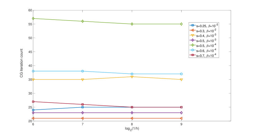
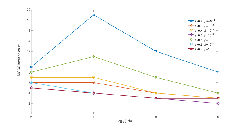
Figure 1. The top and bottom panels respectively show the iteration counts for CG and MGCG with respect to the mesh-size. As expected, we observe the iteration count to be independent of the mesh-size for CG and this iteration count decreases in case of MGCG as the mesh-size decreases, except for, perhaps, the transition from two-to three grids; since the base case is $h=2^{-5}$, we see in some cases a slight increase in MGCG iteration MGCG from $h=2^{-6}$ to $h=2^{-7}$.

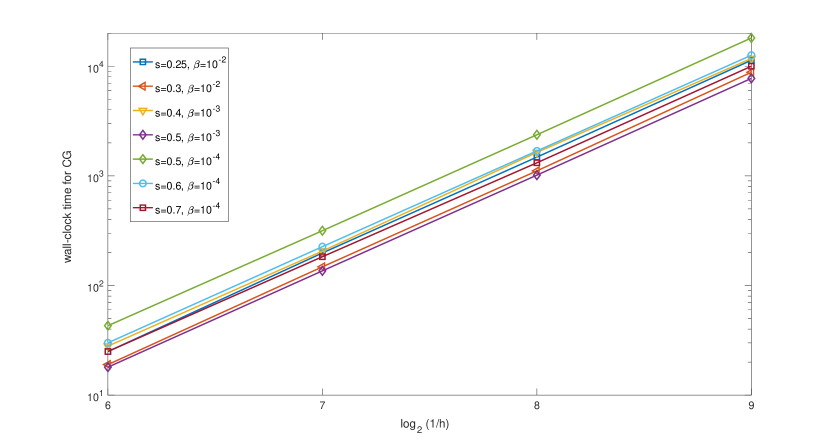
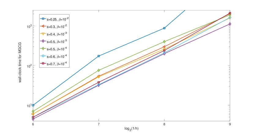
Figure 2. The top and bottom panels respectively show the wall clock time for CG and MGCG with respect to the mesh-size. As expected, on the log-log plot we observe a perfectly linear behavior for CG and a sublinear behavior for MGCG (we excluded from range the value marked with * in Table 2, since it only reflects that the machine was forced into much slower swap space).

References

-
[1]
H. Antil, J. Pfefferer, S. Rogovs,
Fractional operators with
inhomogeneous boundary conditions: analysis, control, and discretization,
Commun. Math. Sci. 16 (5) (2018) 1395–1426.
doi:10.4310/CMS.2018.v16.n5.a11.
URL https://doi.org/10.4310/CMS.2018.v16.n5.a11 - [2] C. J. Weiss, B. G. van Bloemen Waanders, H. Antil, Fractional operators applied to geophysical electromagnetics, Geophys. J. Int. 220 (2) (2020) 1242–1259.
- [3] H. Antil, M. D’Elia, C. A. Glusa, C. J. Weiss, B. G. van Bloemen Waanders, A fast solver for the fractional helmholtz equation., Tech. rep., Sandia National Lab.(SNL-NM), Albuquerque, NM (United States) (2019).
- [4] P. Larkin, Developments in direct-field acoustic testing, Sound and Vibration Magazine (2014).
- [5] E. Auger, L. D’Auria, M. Martini, B. Chouet, P. Dawson, Real-time monitoring and massive inversion of source parameters of very long period seismic signals: An application to stromboli volcano, italy, Geophysical Research Letters 33 (4) (2006).
- [6] H. Antil, S. Bartels, Spectral Approximation of Fractional PDEs in Image Processing and Phase Field Modeling, Comput. Methods Appl. Math. 17 (4) (2017) 661–678.
- [7] H. Antil, Z. W. Di, R. Khatri, Bilevel optimization, deep learning and fractional laplacian regularizatin with applications in tomography, Inverse Problems 36 (6) (2020) 064001. doi:10.1088/1361-6420/ab80d7.
- [8] H. Antil, E. Otárola, A FEM for an Optimal Control Problem of Fractional Powers of Elliptic Operators, SIAM J. Control Optim. 53 (6) (2015) 3432–3456. doi:10.1137/140975061.
- [9] P. Stinga, J. Torrea, Extension problem and Harnack’s inequality for some fractional operators, Comm. Part. Diff. Eqs. 35 (11) (2010) 2092–2122. doi:10.1080/03605301003735680.
- [10] L. Caffarelli, L. Silvestre, An extension problem related to the fractional Laplacian, Comm. Part. Diff. Eqs. 32 (7-9) (2007) 1245–1260. doi:10.1080/03605300600987306.
- [11] S. Dohr, C. Kahle, S. Rogovs, P. Swierczynski, A FEM for an optimal control problem subject to the fractional laplace equation, Calcolo 56 (4) (2019) 37.
- [12] T. Kato, Note on fractional powers of linear operators, Proceedings of the Japan Academy 36 (3) (1960) 94–96.
- [13] A. Bonito, J. Pasciak, Numerical approximation of fractional powers of elliptic operators, Math. Comp. 84 (295) (2015) 2083–2110. doi:10.1090/S0025-5718-2015-02937-8.
- [14] G. Heidel, V. Khoromskaia, B. N. Khoromskij, V. Schulz, Tensor approach to optimal control problems with fractional d-dimensional elliptic operator in constraints, arXiv preprint arXiv:1809.01971 (2018).
-
[15]
H. Antil, M. Warma, Optimal control
of fractional semilinear PDEs, ESAIM Control Optim. Calc. Var. 26 (2020)
Paper No. 5, 30.
doi:10.1051/cocv/2019003.
URL https://doi.org/10.1051/cocv/2019003 -
[16]
M. D’Elia, C. Glusa, E. Otárola,
A priori error estimates for the
optimal control of the integral fractional Laplacian, SIAM J. Control
Optim. 57 (4) (2019) 2775–2798.
doi:10.1137/18M1219989.
URL https://doi.org/10.1137/18M1219989 -
[17]
H. Antil, M. Warma, Optimal control
of the coefficient for the regional fractional -Laplace equation:
approximation and convergence, Math. Control Relat. Fields 9 (1) (2019)
1–38.
doi:10.3934/mcrf.2019001.
URL https://doi.org/10.3934/mcrf.2019001 - [18] H. Antil, M. Warma, Optimal control of the coefficient for fractional -L aplace equation: Approximation and convergence, RIMS Kôkyûroku 2090 (2018) 102–116.
-
[19]
H. Antil, R. Khatri, M. Warma,
External optimal control of
nonlocal PDEs, Inverse Problems 35 (8) (2019) 084003, 35.
doi:10.1088/1361-6420/ab1299.
URL https://doi.org/10.1088/1361-6420/ab1299 -
[20]
H. Antil, D. Verma, M. Warma,
External optimal control of
fractional parabolic PDEs, ESAIM Control Optim. Calc. Var. 26 (2020).
doi:10.1051/cocv/2020005.
URL https://doi.org/10.1051/cocv/2020005 -
[21]
M. Ainsworth, C. Glusa,
Aspects of an adaptive
finite element method for the fractional Laplacian: a priori and a
posteriori error estimates, efficient implementation and multigrid solver,
Comput. Methods Appl. Mech. Engrg. 327 (2017) 4–35.
doi:10.1016/j.cma.2017.08.019.
URL https://doi.org/10.1016/j.cma.2017.08.019 - [22] A. Borzì, V. Schulz, Computational optimization of systems governed by partial differential equations, Vol. 8 of Computational Science & Engineering, Society for Industrial and Applied Mathematics (SIAM), Philadelphia, PA, 2012.
- [23] A. Drăgănescu, T. Dupont, Optimal order multilevel preconditioners for regularized ill-posed problems, Mathematics of computation 77 (264) (2008) 2001–2038.
- [24] L. Tartar, An introduction to Sobolev spaces and interpolation spaces, Vol. 3 of Lecture Notes of the Unione Matematica Italiana, Springer, Berlin, 2007.
- [25] H. Antil, J. Pfefferer, A short matlab implementation of fractional poisson equation with nonzero boundary conditions, Tech. rep., Technical report (2017).
- [26] A. T. Barker, A. Drăgănescu, Algebraic multigrid preconditioning of the hessian in optimization constrained by a partial differential equation, Numerical Linear Algebra with Applications (2020). doi:10.1002/nla.2333.
-
[27]
S. C. Brenner, L. Scott, The
Mathematical Theory of Finite Element Methods, 3rd Edition, Vol. 15 of Texts
in Applied Mathematics, Springer, New York, 2008.
doi:10.1007/978-0-387-75934-0.
URL http://dx.doi.org/10.1007/978-0-387-75934-0