Distributed Constraint-Coupled Optimization via
Primal Decomposition over Random Time-Varying Graphs

Abstract

The paper addresses large-scale, convex optimization problems that need to be solved in a distributed way by agents communicating according to a random time-varying graph. Specifically, the goal of the network is to minimize the sum of local costs, while satisfying local and coupling constraints. Agents communicate according to a time-varying model in which edges of an underlying connected graph are active at each iteration with certain non-uniform probabilities. By relying on a primal decomposition scheme applied to an equivalent problem reformulation, we propose a novel distributed algorithm in which agents negotiate a local allocation of the total resource only with neighbors with active communication links. The algorithm is studied as a subgradient method with block-wise updates, in which blocks correspond to the graph edges that are active at each iteration. Thanks to this analysis approach, we show almost sure convergence to the optimal cost of the original problem and almost sure asymptotic primal recovery without resorting to averaging mechanisms typically employed in dual decomposition schemes. Explicit sublinear convergence rates are provided under the assumption of diminishing and constant step-sizes. Finally, an extensive numerical study on a plug-in electric vehicle charging problem corroborates the theoretical results.

I Introduction

Large-scale systems consisting of several independent control systems can be found in numerous contexts ranging from smart grids to autonomous vehicles and cooperative robotics. In order to perform cooperative control tasks, such systems (or agents) must employ their computation capabilities and collaborate with each other by means of neighboring communication, without resorting to a centralized computing unit. These cooperative tasks can be often formulated as distributed optimization problems consisting of a large number of decision variables, each one associated to an agent in the network and satisfying private constraints. Furthermore, a challenging feature of such optimization problems is that all the decision variables are intertwined by means of a global coupling constraint, that can be used to model, e.g., formation maintenance requirements or a total budget that must not be exceeded. This set-up is referred to as constraint coupled optimization.

The majority of the literature on distributed optimization has focused on a framework in which, differently from the constraint-coupled set-up, cost functions and constraints depend on the same, common decision variable, and agents aim for consensual optimal solutions. An exemplary, non-exhaustive list of works for this optimization set-up is [2, 3, 4, 5, 6, 7, 8]. Only recently has the constraint-coupled set-up gathered more attention from our community, due to its applicability in control. In [9] consensus-based dual decomposition is combined with a primal recovery mechanism, whereas [10] considers a distributed dual algorithm based on proximal minimization. In [11] a distributed algorithm based on successive duality steps is proposed. Differently from [9, 10], which employ running averages for primal recovery, [11] can guarantee feasibility of primal iterates without averaging schemes. In [12] a consensus-based primal-dual perturbation algorithm is proposed to solve smooth constraint-coupled optimization problems. A distributed saddle-point algorithm with Laplacian averaging is proposed in [13] for a class of min-max problems. In [14], a distributed algorithm based on cutting planes is formulated. Recently, in [15] a primal-dual algorithm with constant step-size is proposed under smoothness assumption of both costs and constraints. The works in [16, 17, 18] consider a similar set-up, but the proposed algorithms strongly rely on the sparsity pattern of the coupling constraints. Linear constraint-coupled problem set-ups have been also tackled by means of distributed algorithms based on the Alternating Direction Method of Multipliers (ADMM). In [19] the so-called consensus-ADMM is applied to the dual problem formulation, which is then tailored for an application in Model Predictive Control by [20]. In [21] an ADMM-based algorithm is proposed and analyzed using an operator theory approach while in [22] an augmented Lagrangian approach equipped with a tracking mechanism is proposed. However, the last two approaches require agents to perform multiple communication rounds to converge in a neighborhood of an optimal solution. In [23] ADMM is combined with a tracking mechanism to design a distributed algorithm with exact convergence to an optimal solution.

The analysis of our algorithm for random time-varying graphs builds on randomized block subgradient methods, therefore let us recall some related works from the centralized literature. A survey on block coordinate methods is given in [24], while a unified framework for nonsmooth problems can be found [25]. In [26], a randomized block coordinate descent method is formulated, whereas [27] investigates a stochastic block mirror descent approach with random block updates. In [28], a distributed algorithm for a linearly constrained problem is analyzed with coordinate descent methods. This technique is also used in [29], which considers a constraint-coupled problem. However, the approach used in [28, 29] only allow for a single pair of agents updating at a time and requires smooth cost functions.

In this paper, we propose a distributed algorithm to solve nonsmooth constraint-coupled optimization problems over random, time-varying communication networks. We consider a communication model in which edges of an underlying, connected graph have a certain probability of being active at each time step. The proposed algorithm consists in a two-step procedure in which agents first solve a local optimization problem and then update a vector representing the local allocation of total resource. The algorithmic structure is inspired to the algorithm for fixed graphs in [11]. However, the line of analysis proposed in [11] hampers extension to time-varying graphs. Therefore, in this paper, we develop a new theoretical analysis to deal with the significant challenges arising in the time-varying context. In particular, this method is interpreted as a primal decomposition scheme applied to an equivalent, relaxed version of the target constraint-coupled problem. For this scheme, we prove that almost surely the objective value converges to the optimal cost, and any limit point of the local solution estimates is an optimal (feasible) solution. Moreover, we prove a sublinear convergence rate of the objective value under the assumption of constant or diminishing step-size. As for constant step-size, convergence to a neighborhood of the solution is attained with a rate $O(1/\sqrt{t})$, while for a diminishing step-size of the type $1/t$, exact convergence is attained with rate $O(1/\log(t))$. To show these results, we employ a graph-induced change of variables to derive an equivalent, unconstrained problem formulation. This allows us to recast the distributed algorithm as a randomized block subgradient method in which blocks correspond to edges in the graph. As a side result, we also provide an almost sure convergence result for a block subgradient method in which (multiple) blocks are drawn according to non-uniform probabilities. This generalized block subgradient method results into updates in which different combinations of multiple blocks can be chosen. To the best of our knowledge, these nontrivial challenges have not been addressed so far in the block subgradient literature. A thorough comparison of the contributions provided in this paper with existing work will be performed in light of the analysis provided in Section IV.

The paper is organized as follows. In Section II, we introduce the distributed optimization set-up and we describe the proposed distributed algorithm. In Section III, we provide intermediate results on a (centralized) block subgradient method, which are then used in Section IV for the analysis of the distributed algorithm. Convergence rates and a discussion on algorithm tuning are enclosed in Section V. Finally, in Section VI, an extensive numerical study on a control application is presented.

Notation

The symbols $\mathbf{0}$ and $\mathbf{1}$ denote the vector of zeros and ones respectively. The $n\times n$ identity matrix is denoted by $I_{n}$. Where the size of the matrix is clear from the context, we drop the subscript $n$. Given a vector $\mathbf{x}\in^{n}$ and a positive definite matrix $W\in^{n\times n}$, we denote by $\|\mathbf{x}\|_{W}=\sqrt{\mathbf{x}^{\top}W\mathbf{x}}$ the norm of $\mathbf{x}$ weighted by $W$, which we also term $W$-norm. Given two vectors $\mathbf{x},\mathbf{y}\in^{n}$ we write $\mathbf{x}\leq\mathbf{y}$ (and consistently for other sides) to denote component-wise inequalities. The symbol $\otimes$ denotes the Kronecker product. Given a convex function $f(\mathbf{x}):^{n}\rightarrow$ and a vector $\bar{\mathbf{x}}\in^{n}$, we denote by $\widetilde{\nabla}f(\bar{\mathbf{x}})$ a subgradient of $f$ at $\bar{\mathbf{x}}$. Given a vector $\mathbf{z}$ arranged in $m$ blocks, its $\ell$-th block (or portion) is denoted by $\mathbf{z}_{\ell}$ or, interchangeably, by $[\mathbf{z}]_{\ell}$, and the complete vector is written $\mathbf{z}=(\mathbf{z}_{1},\ldots,\mathbf{z}_{m})$.

II Optimization Set-up and Distributed Algorithm

In this section, we formalize the investigated problem and network set-up. Then, we present the proposed distributed algorithm together with its convergence result. Finally, we recall some preliminaries for the subsequent analysis.

II-A Distributed Constraint-Coupled Optimization

We deal with a network of $N$ agents that must solve a constraint-coupled optimization problem, which can be stated as follows

$$\begin{split}\min_{\mathbf{x}_{1},\ldots,\mathbf{x}_{N}}\>&\>\sum_{i=1}^{N}f_{i}(\mathbf{x}_{i})\\ \textnormal{subj. to}\>&\>\sum_{i=1}^{N}\mathbf{g}_{i}(\mathbf{x}_{i})\leq\mathbf{0},\\ &\>\mathbf{x}_{i}\in X_{i},\hskip 28.45274pti\in\{1,\ldots,N\},\end{split}$$ (1)

where $\mathbf{x}_{1},\ldots,\mathbf{x}_{N}$ are the decision variables with each $\mathbf{x}_{i}\in^{n_{i}}$, $n_{i}\in{\mathbb{N}}$. Moreover, for all $i\in\{1,\ldots,N\}$, $f_{i}:^{n_{i}}\rightarrow$ depends only on $\mathbf{x}_{i}$, $X_{i}\subset^{n_{i}}$ is the constraint set associated to $\mathbf{x}_{i}$ and $\mathbf{g}_{i}:^{n_{i}}\rightarrow^{S}$ is the $i$-th contribution to the (vector-valued) coupling constraint $\sum_{i=1}^{N}\mathbf{g}_{i}(\mathbf{x}_{i})\leq\mathbf{0}$.

In the considered distributed computation framework, the problem data are assumed to be scattered throughout the network. Agents have only a partial knowledge of the entire problem and must cooperate with each other in order to find a solution. Each agent $i$ is assumed to know only its local constraint $X_{i}$, its local cost $f_{i}$ and its own contribution $\mathbf{g}_{i}$ to the coupling constraints, and is only interested in computing its own portion $\mathbf{x}_{i}^{\star}$ of an optimal solution $(\mathbf{x}_{1}^{\star},\ldots,\mathbf{x}_{N}^{\star})$ of problem (1).

The following two assumptions guarantee that (i) the optimal cost of problem (1) is finite and at least one optimal solution exists, (ii) duality arguments are applicable.

Assumption II.1.

For all $i\in\{1,\ldots,N\}$, the set $X_{i}$ is non-empty, convex and compact, the function $f_{i}$ is convex and each component of $\mathbf{g}_{i}$ is a convex function. $\square$

Assumption II.2 (Slater’s constraint qualification).

There exist $\bar{\mathbf{x}}_{1}\in X_{1},\ldots,\bar{\mathbf{x}}_{N}\in X_{N}$ such that $\sum_{i=1}^{N}\mathbf{g}_{i}(\bar{\mathbf{x}}_{i})<\mathbf{0}$. $\square$

II-B Random Time-Varying Communication Model

Agents are assumed to communicate according to a time-varying communication graph, obtained as subset of an underlying graph $\mathcal{G}_{u}=(\{1,\ldots,N\},\mathcal{E}_{u})$, assumed to be undirected and connected, where $\mathcal{E}_{u}\subseteq\{1,\ldots,N\}\times\{1,\ldots,N\}$ is the set of edges. An edge $(i,j)$ belongs to $\mathcal{E}_{u}$ if and only if agents $i$ and $j$ can transmit information to each other, in which case also $(j,i)\in\mathcal{E}_{u}$. In many applications, the communication links are not always active (due, e.g., to temporary unavailability). This is taken into account by considering that each undirected edge $(i,j)\in\mathcal{E}_{u}$ has a probability $\sigma_{ij}\in(0,1]$ of being active. As a result, the actual communication network is a random, time-varying graph $\mathcal{G}^{t}=(\{1,\ldots,N\},\mathcal{E}^{t})$, where $t\in{\mathbb{N}}$ represents a universal time index and $\mathcal{E}^{t}\subseteq\mathcal{E}_{u}$ is the set of active edges at time $t$. The set of neighbors of agent $i$ in $\mathcal{G}^{t}$ is denoted by $\mathcal{N}_{i}^{t}=\left\{j\in\{1,\ldots,N\}\mid(i,j)\in\mathcal{E}^{t}\right\}$. Consistently, the set of neighbors of agent $i$ in the underlying graph $\mathcal{G}_{u}$ is denoted by $\mathcal{N}_{i,u}$.

Let us define $\nu_{ij}^{t}$ as the Bernoulli random variable that is equal to $1$ if $(i,j)\in\mathcal{E}^{t}$ and $0$ otherwise, for all $(i,j)\in\mathcal{E}_{u}$ with $j>i$ and $t\geq 0$. The following assumption is made.

Assumption II.3.

For all $(i,j)\in\mathcal{E}_{u}$ with $j>i$, the random variables $\{\nu_{ij}^{t}\}_{t\geq 0}$ are independent and identically distributed (i.i.d.). Moreover, for all $t\geq 0$, the random variables $\{\nu_{ij}^{t}\}_{(i,j)\in\mathcal{E}_{u},\>j>i}$ are mutually independent. $\square$

A pictorial representation of the time-varying communication model is provided in Figure 1.

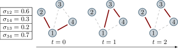
Figure 1: Example of random time-varying network with $N=4$ agents. Active edges are denoted with red lines, while inactive edges are depicted with dashed gray lines. The (connected) underlying graph is the union of all such edges, and the activation probabilities are specified in the table.

II-C Distributed Algorithm Description

Let us now introduce the Distributed Primal Decomposition for Time-Varying graphs (DPD-TV) algorithm to compute an optimal solution $(\mathbf{x}_{1}^{\star},\ldots,\mathbf{x}_{N}^{\star})$ of problem (1). Informally, the algorithm works as follows. Each agent stores and updates a local solution estimate $\mathbf{x}_{i}^{t}\in^{n_{i}}$ and the auxiliary variables $\rho_{i}^{t}\in,\boldsymbol{\mu}_{i}^{t},\mathbf{y}_{i}^{t}\in^{S}$. At the beginning, the variable $\mathbf{y}_{i}^{t}$ is initialized such that $\sum_{i=1}^{N}\mathbf{y}_{i}^{0}=\mathbf{0}$ (e.g., $\mathbf{y}_{i}^{0}=\mathbf{0}$ for all $i$). At each iteration $t$, agents solve a local optimization problem using the current value of $\mathbf{y}_{i}^{t}$. The variables $(\mathbf{x}_{i}^{t},\rho_{i}^{t})$ are set to the primal solution of this problem, where $\mathbf{x}_{i}^{t}$ forms an estimate of $\mathbf{x}_{i}^{\star}$ and $\rho_{i}^{t}$ is a transient violation of the coupling constraints (more details are given in Section II-D). The variable $\boldsymbol{\mu}_{i}^{t}$ is set to the dual solution of the problem and, together with the information gathered from neighbors, is used to update $\mathbf{y}_{i}^{t}$.

Formally, let $\alpha^{t}\geq 0$ denote the step-size and let $M>0$ be a tuning parameter (see Section V-B for a discussion). The next table summarizes the DPD-TV algorithm from the perspective of node $i$, where the notation “$\boldsymbol{\mu}_{i}:$” in (2) means that $\boldsymbol{\mu}_{i}$ is the Lagrange multiplier associated to $\mathbf{g}_{i}(\mathbf{x}_{i})\leq\mathbf{y}_{i}^{t}+\rho_{i}\mathbf{1}$.

Initialization: $\mathbf{y}_{i}^{0}$ such that $\sum_{i=1}^{N}\mathbf{y}_{i}^{0}=\mathbf{0}$

For $t=0,1,2,\ldots$

    Compute $((\mathbf{x}_{i}^{t},\rho_{i}^{t}),\>\boldsymbol{\mu}_{i}^{t})$ as a primal-dual solution of

$$\begin{split}\min_{\mathbf{x}_{i},\rho_{i}}\hskip 34.14322pt&\>f_{i}(\mathbf{x}_{i})+M\rho_{i}\\ \textnormal{subj. to}\>\>\>\boldsymbol{\mu}_{i}:\>&\>\mathbf{g}_{i}(\mathbf{x}_{i})\leq\mathbf{y}_{i}^{t}+\rho_{i}\mathbf{1}\\ &\>\mathbf{x}_{i}\in X_{i},\>\>\rho_{i}\geq 0\end{split}$$ (2)

    Gather $\boldsymbol{\mu}_{j}^{t}$ from $j\in\mathcal{N}_{i}^{t}$ and update

$$\mathbf{y}_{i}^{t+1}=\mathbf{y}_{i}^{t}+\alpha^{t}\sum_{j\in\mathcal{N}_{i}^{t}}\big{(}\boldsymbol{\mu}_{i}^{t}-\boldsymbol{\mu}_{j}^{t}\big{)}$$ (3)

Algorithm DPD-TV

The algorithmic updates of DPD-TV are inspired to the scheme proposed in [11], where different agent states are considered in place of $\mathbf{y}_{i}$. This notational variation reflects the different analysis approach of DPD-TV based on primal decomposition.

Some appealing features of the DPD-TV are worth highlighting. The algorithm naturally preserves privacy of all the agents, in the sense they do not communicate any of their private information (such as the local cost $f_{i}$, the local constraint $X_{i}$ or the local solution estimate $\mathbf{x}_{i}^{t}$). In addition, the algorithm is scalable, i.e., the amount of local computation only depends on the number of neighbors and not on the network size.

In order to state the main result of this paper, let us make the following assumption on the step-size sequence.

Assumption II.4.

The step-size sequence $\{\alpha^{t}\}_{t\geq 0}$, with each $\alpha^{t}\geq 0$, satisfies $\sum_{t=0}^{\infty}\alpha^{t}\!=\!\infty$ and $\sum_{t=0}^{\infty}(\alpha^{t})^{2}\!<\!\infty$. $\square$

Next we provide the convergence properties of DPD-TV. Despite its simple form, the analysis is quite involved and requires several technical tools that will be provided in the forthcoming sections.

Theorem II.5.

Let Assumptions II.1, II.2, II.3 and II.4 hold. Moreover, let $\boldsymbol{\mu}^{\star}$ be an optimal Lagrange multiplier of problem (1) associated to the constraint $\sum_{i=1}^{N}\mathbf{g}_{i}(\mathbf{x}_{i})\leq\mathbf{0}$ and assume $M>\|\boldsymbol{\mu}^{\star}\|_{1}$. Consider a sequence $\{\mathbf{x}_{i}^{t},\rho_{i}^{t}\}_{t\geq 0},\>i\in\{1,\ldots,N\}$ generated by the DPD-TV algorithm with allocation vectors $\mathbf{y}_{i}^{0}$ initialized such that $\sum_{i=1}^{N}\mathbf{y}_{i}^{0}=\mathbf{0}$. Then, almost surely,

1. $\sum_{i=1}^{N}\big{(}f_{i}(\mathbf{x}_{i}^{t})+M\rho_{i}^{t}\big{)}\to f^{\star}$ as $t\to\infty$, where $f^{\star}$ is the optimal cost of (1);

2. every limit point of $\{(\mathbf{x}_{1}^{t},\ldots\,\mathbf{x}_{N}^{t})\}_{t\geq 0}$ is an optimal (feasible) solution of (1). $\square$

In principle, in order to satisfy the assumption $M>\|\boldsymbol{\mu}^{\star}\|_{1}$ in Theorem II.5, knowledge is needed of the dual optimal solution $\boldsymbol{\mu}^{\star}$. However, this is not necessary in practice, as a lower bound of $M$ can be efficiently computed when a Slater point is known. In Section V-B, we provide a sufficient condition to select valid values of $M$ without any knowledge on $\boldsymbol{\mu}^{\star}$.

Note also that the algorithm does not employ any averaging mechanism typically appearing in dual algorithms when the cost functions are not strictly convex. However, thanks to the primal decomposition approach, we are still able to prove asymptotic feasibility (other than optimality) of the sequence $\{(\mathbf{x}_{1}^{t},\ldots\,\mathbf{x}_{N}^{t})\}_{t\geq 0}$. As shown in Section VI-C, the absence of running averages allows for faster practical convergence, compared to existing methods.

Remark II.6 (Computational load of DPD-TV).

As many of duality-based distributed algorithms, DPD-TV requires the repeated solution of local optimization problems and also to compute the Lagrange multiplier $\boldsymbol{\mu}_{i}^{t}$ associated to the inequality constraint. As a matter of fact, the computation of $\boldsymbol{\mu}_{i}^{t}$ has a minor impact on the computational load. Indeed, if a solver based on interior-point methods is used, it will provide $\boldsymbol{\mu}_{i}^{t}$ as a byproduct of the solution process. Alternatively, denoting $(\mathbf{x}_{i}^{t},\rho_{i}^{t})$ the optimal solution at time $t$, a Lagrange multiplier $\boldsymbol{\mu}_{i}^{t}$ can be easily computed as the solution of a linear system with positivity constraints (cf. [30, Proposition 5.1.5]), i.e.,

$$\boldsymbol{\mu}_{i,s}(\mathbf{g}_{i,s}(\mathbf{x}_{i}^{t})-\mathbf{y}_{i,s}^{t}-\rho_{i}^{t})=0\quad\forall\>s,\hskip 8.5359pt\text{with }\boldsymbol{\mu}_{i}\geq 0. \square$$

II-D Preliminaries on Relaxation and Primal Decomposition

In this subsection we recall two preliminary building blocks for the algorithm analysis, namely the relaxation and the primal decomposition approach for problem (1) originally introduced in [31, 30, 11, 32]. In a primal decomposition scheme, also called right-hand side allocation, the coupling constraints $\sum_{i=1}^{N}\mathbf{g}_{i}(\mathbf{x}_{i})\leq\mathbf{0}$ are interpreted as a limited resource to be shared among nodes. A two-level structure is formulated, where independent subproblems, with a fixed resource allocation, are “coordinated” by a master problem determining the optimal resource allocation. We will apply such approach to an equivalent, relaxed version of problem (1). Formally, consider the following modified version of problem (1),

$$\begin{split}\min_{\mathbf{x}_{1},\ldots,\mathbf{x}_{N},\rho}\>&\>\sum_{i=1}^{N}f_{i}(\mathbf{x}_{i})+M\rho\\ \textnormal{subj. to}\>&\>\sum_{i=1}^{N}\mathbf{g}_{i}(\mathbf{x}_{i})\leq\rho\mathbf{1},\\ &\>\rho\geq 0,\>\>\mathbf{x}_{i}\in X_{i},\hskip 14.22636pti\in\{1,\ldots,N\},\end{split}$$ (4)

where $M>0$ is a scalar and we added the scalar optimization variable $\rho$. In principle, the new variable allows for a violation of the coupling constraints (in this sense, we say that problem (4) is a relaxed version of problem (1)). However, if the constant $M$ appearing in the penalty term $M\rho$ is large enough, problem (4) is equivalent to (1), as we recall in the next lemma.

Lemma II.7 ([11], Proposition III.3).

Let Assumptions II.1 and II.2 hold. Moreover, let $M$ be such that $M>\|\boldsymbol{\mu}^{\star}\|_{1}$, with $\boldsymbol{\mu}^{\star}\in^{S}$ an optimal Lagrange multiplier for problem (1) associated to the constraint $\sum_{i=1}^{N}\mathbf{g}_{i}(\mathbf{x}_{i})\leq\mathbf{0}$. Then, the optimal solutions of the relaxed problem (4) are in the form $(\mathbf{x}_{1}^{\star},\ldots,\mathbf{x}_{N}^{\star},0)$, where $(\mathbf{x}_{1}^{\star},\ldots,\mathbf{x}_{N}^{\star})$ is an optimal solution of (1), i.e., the solutions of (4) must have $\rho=0$. Moreover, the optimal costs of (4) and (1) are equal. $\square$

The primal decomposition scheme applied to problem (4) can be formulated as follows. For all $i\in\{1,\ldots,N\}$ and $\mathbf{y}_{i}\in^{S}$, the $i$-th subproblem is

$$\begin{split}p_{i}(\mathbf{y}_{i})\triangleq\min_{\mathbf{x}_{i},\rho_{i}}\>&\>f_{i}(\mathbf{x}_{i})+M\rho_{i}\\ \textnormal{subj. to}\>&\>\mathbf{g}_{i}(\mathbf{x}_{i})\leq\mathbf{y}_{i}+\rho_{i}\mathbf{1}\\ &\>\rho_{i}\geq 0,\>\>\mathbf{x}_{i}\in X_{i},\end{split}$$ (5)

where $\mathbf{y}_{i}\in^{S}$ is a (given) local allocation for node $i$ and $p_{i}(\mathbf{y}_{i})$ denotes the optimal cost as a function of $\mathbf{y}_{i}$. The local allocations are “coordinated” by the master problem, i.e.,

$$\begin{split}\min_{\mathbf{y}_{1},\ldots,\mathbf{y}_{N}}\>&\>\sum_{i=1}^{N}p_{i}(\mathbf{y}_{i})\\ \textnormal{subj. to}\>&\>\sum_{i=1}^{N}\mathbf{y}_{i}=\mathbf{0}.\end{split}$$ (6)

In the next, we will denote the cost function of (6) as $p(\mathbf{y})=\sum_{i=1}^{N}p_{i}(\mathbf{y}_{i})$, where $\mathbf{y}=(\mathbf{y}_{1},\ldots,\mathbf{y}_{N})\in^{SN}$. Notice that subproblem (5) is always feasible for all $\mathbf{y}_{i}\in^{S}$. The following lemma establishes the equivalence between the master problem (6) and the relaxed problem (4).

Lemma II.8 ([31]).

Let Assumption II.1 hold. Then, problems (4) and (6) are equivalent, in the sense that (i) the optimal costs are equal, (ii) if $(\mathbf{x}_{1}^{\star},\ldots,\mathbf{x}_{N}^{\star})$ is an optimal solution of (4) and $(\mathbf{y}_{1}^{\star},\ldots,\mathbf{y}_{N}^{\star})$ is an optimal solution of (6), then $(\mathbf{x}_{i}^{\star},0)$ is an optimal solution of (5), with $\mathbf{y}_{i}=\mathbf{y}_{i}^{\star}$, for all $i\in\{1,\ldots,N\}$. $\square$

Thanks to Lemma II.7 and Lemma II.8, solving problem (1) is equivalent to solving problem (6). We will show that indeed the DPD-TV algorithm solves (6), thereby indirectly providing a solution to (1). Consider now the update (3). Owing to the discussion in [30, Section 5.4.4], can be rewritten as

$$\mathbf{y}_{i}^{t+1}=\mathbf{y}_{i}^{t}-\alpha^{t}\sum_{j\in\mathcal{N}_{i}^{t}}\big{(}\widetilde{\nabla}p_{i}(\mathbf{y}_{i}^{t})-\widetilde{\nabla}p_{j}(\mathbf{y}_{j}^{t})\big{)},$$

for $i\in\{1,\ldots,N\}$. This equivalent form highlights that, at each iteration $t$, agents adjust their local allocation $\mathbf{y}_{i}^{t}$ by performing a subgradient-like step, based only on local and neighboring information. Note also that, by direct calculation, using the fact that the underlying graph is undirected, one can see that $\sum_{i=1}^{N}\mathbf{y}_{i}^{t}=\sum_{i=1}^{N}\mathbf{y}_{i}^{0}=\mathbf{0}$ for all $t$, which means that the allocation sequence produced by the algorithm satisfies the constraint $\sum_{i=1}^{N}\mathbf{y}_{i}=\mathbf{0}$ appearing in problem (6) at each time step $t$.

Remark II.9 (On the variables $\rho_{i}$).

Finally, let us comment on the role of the variables $\rho_{i}$ appearing in problem (2). If we impose $\rho_{i}=0$, problem (2) may become infeasible for some values of $\mathbf{y}_{i}$. Thus, the variable $\rho_{i}$ guarantees that the agents can always select a sufficiently large value of $\rho_{i}$ in order to satisfy the constraint $\mathbf{g}_{i}(\mathbf{x}_{i})\leq\mathbf{y}_{i}^{t}+\rho_{i}\mathbf{1}$. By Theorem II.5, the sequences $\{\rho_{i}^{t}\}_{t\geq 0}$ converge to zero and, hence, they represent only a temporary violation.

Strictly speaking, if one wanted to apply the primal decomposition method directly to problem (1) (or, equivalently, to problem (4) with $\rho_{i}=0$), additional constraints of the type $\mathbf{y}_{i}\in Y_{i}$, $i\in\{1,\ldots,N\}$ should be included in problem (6), with each $Y_{i}$ being the set of $\mathbf{y}_{i}$ such that the subproblems are feasible [30, Section 6.4.2]. However, as it will be clear from the forthcoming analysis, this would prevent us from obtaining a purely distributed scheme (in particular, problem (14) would not be unconstrained). $\square$

III Randomized Block Subgradient for Convex Problems

In this section, we formulate a (centralized) randomized block subgradient method for convex problems and formally prove its convergence. This algorithm will be used in the next to solve an equivalent form of problem (6), where the update of blocks is associated to the activation of edges in the graph. The results provided here hold for a more general class of optimization problems, therefore for this section we temporarily stop our discussion to formalize and analyze the randomized block subgradient method. Subsequently, we loop back to the main focus of this work and apply the results of this section for the analysis of DPD-TV.

Let us consider the unconstrained convex problem

$$\begin{split}\min_{\theta\in^{m}}\>&\>\varphi(\theta),\end{split}$$ (7)

where $\theta$ is the optimization variable and $\varphi:^{m}\rightarrow$ is a convex function. We assume that problem (7) has finite optimal cost, denoted by $\varphi^{\star}$, and that (at least) an optimal solution $\theta^{\star}\in^{m}$ exists, such that $\varphi^{\star}=\varphi(\theta^{\star})$.

Let us consider a partition of ^m into $B\in{\mathbb{N}}$ parts, i.e., ${}^{m}=^{m_{1}}\times\cdots\times^{m_{B}}$, such that $m=\sum_{\ell=1}^{B}m_{\ell}$. Therefore, the optimization variable is the stack of $B$ blocks,

$$\theta=(\theta_{1},\ldots,\theta_{B}),$$

where $\theta_{\ell}\in^{m_{\ell}}$ for all $\ell\in\{1,\ldots,B\}$. Now, we develop a subgradient method with block-wise updates to solve problem (7). At each iteration $t\in{\mathbb{N}}$, each block $\ell$ is updated with a probability $\sigma_{\ell}>0$.

We stress that according to the considered model, blocks can have different update probabilities and multiple blocks can be updated simultaneously.

For all $t$, we denote by $B^{t}\subseteq\{1,\ldots,B\}$ the index set of the blocks selected at time $t$. For all $\ell\in\{1,\ldots,B\}$ and $t\geq 0$, let us define $\nu_{\ell}^{t}$ as the Bernoulli random variable that is equal to $1$ if $\ell\in B^{t}$ and $0$ otherwise. The following assumption is made (compare with Assumption II.3).

Assumption III.1.

For all $\ell\in\{1,\ldots,B\}$, the random variables $\{\nu_{\ell}^{t}\}_{t\geq 0}$ are independent and identically distributed (i.i.d.). Moreover, for all $t\geq 0$, the random variables $\{\nu_{\ell}^{t}\}_{\ell\in\{1,\ldots,B\}}$ are mutually independent. $\square$

The algorithm considered here is based on a subgradient method. However, at each iteration $t$, only the blocks in $B^{t}$ are updated, i.e.,

$$\theta_{\ell}^{t+1}=\begin{cases}\theta_{\ell}^{t}-\alpha^{t}[\widetilde{\nabla}\varphi(\theta^{t})]_{\ell},\hskip 14.22636pt&\text{if }\ell\in B^{t},\\ \theta_{\ell}^{t},&\text{if }\ell\notin B^{t},\end{cases}$$ (8)

where $\alpha^{t}$ is the step-size. Note that algorithm (8) allows for multiple block updates at once and, furthermore, blocks have non-uniform update probabilities. To the best of our knowledge, this general block-subgradient method has not been studied in the literature. Therefore, we now provide the convergence proof for algorithm (8).

Theorem III.2.

Let Assumption III.1 hold and let the step-size sequence $\{\alpha^{t}\}_{t\geq 0}$ satisfy Assumption II.4. Moreover, assume the subgradients of $\varphi$ are block-wise bounded, i.e., assume for all $\ell\in\{1,\ldots,B\}$ there exists $C_{\ell}>0$ such that $\|[\widetilde{\nabla}\varphi(\theta)]_{\ell}\|\leq C_{\ell}$ for all $\theta\in^{m}$. Consider a sequence $\{\theta^{t}\}_{t\geq 0}$ generated by algorithm (8), initialized at any $\theta^{0}\in^{m}$. Then, almost surely, it holds

$$\operatornamewithlimits{lim\vphantom{p}}_{t\to\infty}\varphi(\theta^{t})=\varphi^{\star}.$$

Proof.

To keep the notation light, let us denote the computed subgradients by $\beta^{t}\triangleq\widetilde{\nabla}\varphi(\theta^{t})$. Each block $\ell$ is denoted by $\beta_{\ell}^{t}=[\widetilde{\nabla}\varphi(\theta^{t})]_{\ell}$. Moreover, for all $\ell\in\{1,\ldots,B\}$, let us define the matrix $U_{\ell}\in^{m\times m}$, obtained by setting to zero in the identity matrix all the blocks on the diagonal, except for the $\ell$-th block. Thus, when applied to a vector $\theta\in^{m}$, all the blocks other than the $\ell$-th one are set to zero, i.e.,

$$[U_{\ell}\theta]_{\kappa}=\begin{cases}\theta_{\ell}&\text{if }\kappa=\ell,\\ \mathbf{0}&\text{otherwise},\end{cases}\hskip 14.22636pt\forall\>\kappa\in\{1,\ldots,B\}.$$

Moreover, for the sake of analysis, let us define

$$W\triangleq\operatorname{diag}\Big{(}\frac{1}{\sigma_{1}}I_{m_{1}},\>\ldots,\>\frac{1}{\sigma_{B}}I_{m_{B}}\Big{)},$$

where $\operatorname{diag}(\cdot)$ is the (block) diagonal operator and we recall that $I_{m_{\ell}}$ is the $m_{\ell}\times m_{\ell}$ identity matrix. Note that $W$ is positive definite, thus we can consider the weighted norm $\|\theta\|_{W}$, for which, by definition, it holds

$$\|\theta\|_{W}^{2}=\sum_{\ell=1}^{B}\frac{\|\theta_{\ell}\|^{2}}{\sigma_{\ell}},\hskip 28.45274pt\theta\in^{m}.$$

Next we analyze algorithm (8). Let us focus on an iteration $t$ and consider any vector $\theta\in^{m}$. As for the activated blocks $\ell\in B^{t}$, it holds

$$\|\theta_{\ell}^{t+1}-\theta_{\ell}\|^{2} =\|\theta_{\ell}^{t}-\alpha^{t}\beta_{\ell}^{t}-\theta_{\ell}\|^{2}$$

$$=\|\theta_{\ell}^{t}-\theta_{\ell}\|^{2}+(\alpha^{t})^{2}\|\beta_{\ell}^{t}\|^{2}$$

$$\hskip 28.45274pt-2\alpha^{t}(\beta_{\ell}^{t})^{\top}\big{(}\theta_{\ell}^{t}-\theta_{\ell}\big{)},$$

$$\leq\|\theta_{\ell}^{t}-\theta_{\ell}\|^{2}+(\alpha^{t})^{2}C_{\ell}^{2}$$

$$\hskip 28.45274pt-2\alpha^{t}U_{\ell}(\beta^{t})^{\top}\big{(}\theta^{t}-\theta\big{)},\hskip 5.69046pt\forall\>\ell\in B^{t},$$

where $\|\beta_{\ell}^{t}\|\leq C_{\ell}$ holds by assumption. As for the other blocks $\ell\notin B^{t}$, we have

$$\|\theta_{\ell}^{t+1}-\theta_{\ell}\|^{2} =\|\theta_{\ell}^{t}-\theta_{\ell}\|^{2},\hskip 28.45274pt\forall\>\ell\notin B^{t}.$$

Let us now write the overall evolution in $W$-norm, i.e.,

$$\|\theta^{t+1}\!\!-\theta\|_{W}^{2} =\sum_{\ell\in B^{t}}\frac{\|\theta_{\ell}^{t+1}-\theta_{\ell}\|^{2}}{\sigma_{\ell}}+\sum_{\ell\notin B^{t}}\frac{\|\theta_{\ell}^{t+1}-\theta_{\ell}\|^{2}}{\sigma_{\ell}}$$

$$\leq\sum_{\ell=1}^{B}\frac{\|\theta_{\ell}^{t}-\theta_{\ell}\|^{2}}{\sigma_{\ell}}+(\alpha^{t})^{2}\sum_{\ell\in B^{t}}\frac{C_{\ell}^{2}}{\sigma_{\ell}}$$

$$\hskip 11.38092pt-2\alpha^{t}\bigg{(}\sum_{\ell\in B^{t}}\frac{1}{\sigma_{\ell}}U_{\ell}\bigg{)}(\beta^{t})^{\top}\big{(}\theta^{t}-\theta\big{)}$$

$$\leq\|\theta^{t}-\theta\|_{W}^{2}+(\alpha^{t})^{2}C$$

$$\hskip 11.38092pt-2\alpha^{t}\bigg{(}\sum_{\ell\in B^{t}}\frac{1}{\sigma_{\ell}}U_{\ell}\bigg{)}(\beta^{t})^{\top}\big{(}\theta^{t}-\theta\big{)},$$ (9)

where $C\triangleq\sum_{\ell=1}^{B}\frac{C_{\ell}^{2}}{\sigma_{\ell}}>0$. Regarding the matrix $\sum_{\ell\in B^{t}}\frac{1}{\sigma_{\ell}}U_{\ell}$ appearing in (9), its expected value is

$${\mathbb{E}}\Bigg{[}\sum_{\ell\in B^{t}}\frac{1}{\sigma_{\ell}}U_{\ell}\Bigg{]}={\mathbb{E}}\Bigg{[}\sum_{\ell=1}^{B}\frac{\nu_{\ell}^{t}}{\sigma_{\ell}}U_{\ell}\Bigg{]}=\sum_{\ell=1}^{B}U_{\ell}=I_{m}.$$ (10)

Now, by taking the conditional expectation of (9) with respect to $\mathcal{F}^{t}=\{\theta^{0},\ldots,\theta^{t}\}$ (namely the sequence generated by algorithm (8) up to iteration $t$), we obtain for all $\theta\in^{m}$ and $t\geq 0$

$${\mathbb{E}}\Big{[}\|\theta^{t+1}\!\!-\theta\|_{W}^{2}\>\big{|}\>\mathcal{F}^{t}\Big{]} \stackrel{{\scriptstyle(a)}}{{\leq}}\|\theta^{t}-\theta\|_{W}^{2}+(\alpha^{t})^{2}C$$

$$\hskip 17.07182pt-2\alpha^{t}(\beta^{t})^{\top}\big{(}\theta^{t}-\theta\big{)},$$

$$\stackrel{{\scriptstyle(b)}}{{\leq}}\|\theta^{t}-\theta\|_{W}^{2}+(\alpha^{t})^{2}C$$

$$\hskip 17.07182pt-2\alpha^{t}\big{(}\varphi(\theta^{t})-\varphi(\theta)\big{)},$$

where in $(a)$ we used (10) and the independence of the drawn blocks from the previous iterations (cf. Assumption III.1), and $(b)$ follows by definition of subgradient of the function $\varphi$. By restricting the above inequality to any optimal solution $\theta^{\star}$ of problem (14), we obtain

$${\mathbb{E}}\Big{[}\|\theta^{t+1}\!\!-\theta^{\star}\|_{W}^{2}\>\big{|}\>\mathcal{F}^{t}\Big{]} \leq\|\theta^{t}-\theta^{\star}\|_{W}^{2}+(\alpha^{t})^{2}C$$

$$\hskip 25.6073pt-2\alpha^{t}\big{(}\varphi(\theta^{t})-\varphi^{\star}\big{)}.$$ (11)

Inequality (11) satisfies the assumptions of [33, Proposition 8.2.10]. Thus, by following the same arguments as in [33, Proposition 8.2.13], we conclude that, almost surely,

$$\operatornamewithlimits{lim\vphantom{p}}_{t\to\infty}\varphi(\theta^{t})=\varphi^{\star}. \square$$

∎

Remark III.3.

By employing a different probabilistic model and by slightly adapting the previous proof, almost sure cost convergence can also be proved for a block subgradient method with single block update, thus complementing, e.g., the results in [27]. $\square$

IV Analysis of DPD-TV

In this section, we provide the analysis of DPD-TV. To this end, we first reformulate problem (6) by properly exploiting the graph structure. This reformulation is then used to show that our distributed algorithm is equivalent to a (centralized) randomized block subgradient method. We finally rely on the results of Section III to prove Theorem II.5.

IV-A Encoding the Coupling Constraints in Cost Function

As already mentioned in Section II-D, a solution of problem (1) can be indirectly obtained by solving problem (6). In order to put problem (6) into a form that is more convenient for distributed computation, let us apply a graph-induced change of variables. Such a manipulation has a twofold benefit: (i) it allows for the suppression and implicit satisfaction of the constraint $\sum_{i=1}^{N}\mathbf{y}_{i}=\mathbf{0}$, (ii) it allows for the application of the randomized block subgradient method to take into account the random activation of edges.

Consider the underlying communication graph $\mathcal{G}_{u}$. Assuming an ordering of the edges, let $\Gamma\in^{|\mathcal{E}_{u}|\times N}$ denote the incidence matrix of $\mathcal{G}_{u}$, where each row (corresponding to an edge in the graph) contains all zero entries except for the column corresponding to the edge tail (equal to $1$), and for the column corresponding to the edge head (equal to $-1$). Namely, if the $k$-th row of $\Gamma$ corresponds to the edge $(i,j)$, then the $(k,\ell)$-th entry of $\Gamma$ is

$$(\Gamma)_{k\ell}=\begin{cases}1&\text{if }\ell=i,\\ -1\hskip 5.69046pt&\text{if }\ell=j,\\ 0&\text{otherwise},\end{cases}$$

for all $\ell\in\{1,\ldots,N\}$. For all $(i,j)\in\mathcal{E}_{u}$, let $\mathbf{z}_{(ij)}\in^{S}$ be a vector associated to the edge $(i,j)$ and denote by $\mathbf{z}\in^{S|\mathcal{E}_{u}|}$ the vector stacking all $\mathbf{z}_{(ij)}$, with the same ordering as in $\Gamma$. Consider the change of variables for problem (6) defined through the following linear mapping

$$\mathbf{y} =\Pi\mathbf{z},\hskip 28.45274pt\mathbf{z}\in^{S|\mathcal{E}_{u}|},$$ (12)

where the matrix $\Pi$ is defined as

$$\Pi\triangleq(\Gamma^{\top}\otimes I_{S})\in^{SN\times S|\mathcal{E}_{u}|}.$$ (13)

By using the properties of the Kronecker product, the blocks of $\mathbf{y}$ can be written as

$$\mathbf{y}_{i}=[\Pi\mathbf{z}]_{i}=\sum_{j\in\mathcal{N}_{i,u}}\!(\mathbf{z}_{(ij)}-\mathbf{z}_{(ji)}),\hskip 14.22636pt\forall\>i\in\{1,\ldots,N\}.$$

The next lemma formalizes the fact that the change of variable (12) implicitly encodes the constraint $\sum_{i=1}^{N}\mathbf{y}_{i}=\mathbf{0}$.

Lemma IV.1.

The matrix $\Pi$ in (13) satisfies:

• $\sum_{i=1}^{N}[\Pi\mathbf{z}]_{i}=\mathbf{0}$ for all $\mathbf{z}\in^{S|\mathcal{E}_{u}|}$;

• for all $\tilde{\mathbf{y}}\in^{SN}$ satisfying $\sum_{i=1}^{N}\tilde{\mathbf{y}}_{i}=\mathbf{0}$ there exists $\tilde{\mathbf{z}}\in^{S|\mathcal{E}_{u}|}$ such that $\tilde{\mathbf{y}}=\Pi\tilde{\mathbf{z}}$.

Proof.

To prove (i), we see that

$$\sum_{i=1}^{N}[\Pi\mathbf{z}]_{i} =(\mathbf{1}^{\top}\otimes I_{S})\Pi\mathbf{z}$$

$$=(\mathbf{1}^{\top}\otimes I_{S})(\Gamma^{\top}\otimes I_{S})\mathbf{z}$$

$$=\big{(}(\Gamma\otimes I_{S})(\mathbf{1}\otimes I_{S})\big{)}^{\top}\mathbf{z}$$

$$\stackrel{{\scriptstyle(a)}}{{=}}\big{(}(\Gamma\mathbf{1})\otimes I_{S}\big{)}^{\top}\mathbf{z}$$

$$\stackrel{{\scriptstyle(b)}}{{=}}\big{(}\mathbf{0}\otimes I_{S}\big{)}^{\top}\mathbf{z}=\mathbf{0},$$

where in $(a)$ we used the fact $(A\otimes B)(C\otimes D)=(AC)\otimes(BD)$ since the matrix dimensions are compatible, and $(b)$ follows by the property $\Gamma\mathbf{1}=\mathbf{0}$ of incidence matrices.

To prove (ii), let $\tilde{\mathbf{y}}\in^{SN}$ be such that $\sum_{i=1}^{N}\tilde{\mathbf{y}_{i}}=\mathbf{0}$, or, equivalently, $(\mathbf{1}^{\top}\otimes I_{S})\tilde{\mathbf{y}}=\mathbf{0}$. Let us first show that $\mathbf{v}^{\top}\tilde{\mathbf{y}}=0$ for all $\mathbf{v}\in\operatorname{Ker}(\Pi^{\top})$. To this end, take $\mathbf{v}\in\operatorname{Ker}(\Pi^{\top})$. Since $\mathcal{G}_{u}$ is connected, then $\operatorname{rank}(\Gamma)=N-1$. Thus, by the properties of the Kronecker product, it holds

$$\operatorname{rank}(\Pi^{\top}) =\operatorname{rank}(\Gamma\otimes I_{S})$$

$$=\operatorname{rank}(\Gamma)\operatorname{rank}(I_{S})$$

$$=(N-1)S.$$

Moreover, by the Rank-Nullity Theorem, it holds

$$\dim\operatorname{Ker}(\Pi^{\top}) =SN-\operatorname{rank}(\Pi^{\top})=S.$$

But since the columns of $(\mathbf{1}\otimes I_{S})\in^{SN\times S}$ are linearly independent, and since the point (i) of the lemma implies that they belong to $\operatorname{Ker}(\Pi^{\top})$, it follows that they are actually a basis of $\operatorname{Ker}(\Pi^{\top})$, so that the vector $\mathbf{v}$ can be written as $\mathbf{v}=(\mathbf{1}\otimes I_{S})\boldsymbol{\lambda}$, for some $\boldsymbol{\lambda}\in^{S}$. Therefore, it holds

$$\mathbf{v}^{\top}\tilde{\mathbf{y}}=\boldsymbol{\lambda}^{\top}\underbrace{(\mathbf{1}^{\top}\otimes I_{S})\tilde{\mathbf{y}}}_{=\>\mathbf{0}}=0.$$

Thus, since $\mathbf{v}$ is arbitrary, it follows that $\mathbf{v}^{\top}\tilde{\mathbf{y}}=0$ for all $\mathbf{v}\in\operatorname{Ker}(\Pi^{\top})$. By definition of orthogonal complement, this means that $\tilde{\mathbf{y}}\in\operatorname{Ker}(\Pi^{\top})^{\bot}=\operatorname{Im}(\Pi)$. Equivalently, there exists $\tilde{\mathbf{z}}$ such that $\tilde{\mathbf{y}}=\Pi\tilde{\mathbf{z}}$. The proof follows since $\tilde{\mathbf{y}}$ is arbitrary. ∎

We now plug the change of variable (12) into problem (6). Formally, for all $i\in\{1,\ldots,N\}$, define the functions

$$\tilde{p}_{i}\big{(}\{\mathbf{z}_{(ij)},\mathbf{z}_{(ji)}\}_{j\in\mathcal{N}_{i,u}}\big{)}\triangleq p_{i}\big{(}[\Pi\mathbf{z}]_{i}\big{)},\hskip 19.91684pt\mathbf{z}\in^{S|\mathcal{E}_{u}|}.$$

By Lemma IV.1, we directly obtain the following result.

Corollary IV.2.

Problem (6) is equivalent to the unconstrained optimization problem

$$\min_{\mathbf{z}\in S|\mathcal{E}_{u}|}\>\sum_{i=1}^{N}\tilde{p}_{i}\big{(}\{\mathbf{z}_{(ij)},\mathbf{z}_{(ji)}\}_{j\in\mathcal{N}_{i,u}}\big{)},$$ (14)

in the sense that (i) the optimal costs are equal, and (ii) if $\mathbf{z}^{\star}$ is an optimal solution of (14), then $\mathbf{y}^{\star}=\Pi\mathbf{z}^{\star}$ is an optimal solution of (6). $\square$

In the following, we denote the cost function of (14) as $\tilde{p}(\mathbf{z})=\sum_{i=1}^{N}\tilde{p}_{i}\big{(}\{\mathbf{z}_{(ij)},\mathbf{z}_{(ji)}\}_{j\in\mathcal{N}_{i,u}}\big{)}=p(\Pi\mathbf{z})$.

IV-B Equivalence of DPD-TV and Randomized Block Subgradient

Differently from problem (6), its equivalent formulation (14) is unconstrained. Hence, it can be solved via subgradient methods without projections steps. It is possible to exploit the particular structure of problem (14) to recast the random activation of edges as the random update of blocks within a block subgradient method (8) applied to problem (14). We will use the following identifications,

$$\theta=\mathbf{z},\hskip 14.22636pt\text{and}\hskip 14.22636pt\varphi(\theta)=\sum_{i=1}^{N}\tilde{p}_{i}\big{(}\{\mathbf{z}_{(ij)},\mathbf{z}_{(ji)}\}_{j\in\mathcal{N}_{i,u}}\big{)}.$$ (15)

As for the block structure, the mapping is as follows. Each block $\ell\in\{1,\ldots,B\}$ of $\mathbf{z}$, i.e., $\mathbf{z}_{\ell}\in^{2S}$, is associated to an undirected edge $(i,j)\in\mathcal{E}_{u}$, with $j>i$, and is defined as

$$\mathbf{z}_{\ell}=\begin{bmatrix}\mathbf{z}_{(ij)}\\ \mathbf{z}_{(ji)}\end{bmatrix}.$$ (16)

Therefore, there is a total of $B=|\mathcal{E}_{u}|/2$ blocks. At each iteration $t$, each block $\mathbf{z}_{\ell}$ is updated if the corresponding edge $(i,j)\in\mathcal{E}^{t}$, i.e., if $\nu_{ij}^{t}=1$. A pictorial representation of the block structure of $\mathbf{z}$ is provided in Figure 2.

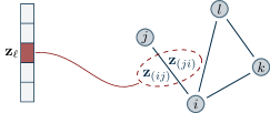
Figure 2: Block structure of the variable $\mathbf{z}$. Each block, say $\ell$, is associated to an undirected edge, say $(i,j)$. The block is the stack of $\mathbf{z}_{(ij)}$, associated to the edge $(i,j)$, and $\mathbf{z}_{(ji)}$ associated to the edge $(j,i)$.

Consistently with the notation of Section III, we use the shorthands $\sigma_{\ell}=\sigma_{ij}$ and $\nu_{\ell}^{t}=\nu_{ij}^{t}$. At each iteration $t$ of algorithm (8), the set $B^{t}$ contains all and only the blocks associated to the edges in $\mathcal{E}^{t}$.

Next, we explicitly write the evolution of the sequences generated by DPD-TV as a function of the sequences generated by the block subgradient method (8). For this purpose, let us write a subgradient of $\tilde{p}$ at any $\mathbf{z}\in^{S|\mathcal{E}_{u}|}$. By definition, it holds $\tilde{p}(\mathbf{z})=p(\Pi\mathbf{z})$. Thus, by using the subgradient property for affine transformations of the domain, it holds

$$\widetilde{\nabla}\tilde{p}(\mathbf{z})=(\Gamma\otimes I_{S})\widetilde{\nabla}p(\Pi\mathbf{z}).$$ (17)

By exploiting the structure of $p$, the $i$-th block of $\widetilde{\nabla}p(\mathbf{y})$ is equal to $\frac{\tilde{\partial}p(\mathbf{y})}{\partial\mathbf{y}_{i}}=\widetilde{\nabla}p_{i}(\mathbf{y}_{i})$. Moreover, since problem (5) enjoys strong duality, a subgradient of $p_{i}$ at $\mathbf{y}_{i}$ can be computed as $\widetilde{\nabla}p_{i}(\mathbf{y}_{i})=-\boldsymbol{\mu}_{i}$, where $\boldsymbol{\mu}_{i}$ is an optimal Lagrange multiplier of problem (5) (cf. [30, Section 5.4.4]). By collecting these facts together with (17), it follows that the blocks of $\widetilde{\nabla}\tilde{p}(\mathbf{z})$ can be computed as

$$\frac{\tilde{\partial}\tilde{p}(\mathbf{z})}{\partial\mathbf{z}_{(ij)}} =\widetilde{\nabla}p_{i}\Big{(}[\Pi\mathbf{z}]_{i}\Big{)}-\widetilde{\nabla}p_{j}\Big{(}[\Pi\mathbf{z}]_{j}\Big{)}$$

$$=\boldsymbol{\mu}_{j}-\boldsymbol{\mu}_{i},\hskip 56.9055pt\forall\>(i,j)\in\mathcal{E}_{u},$$ (18)

where $\frac{\tilde{\partial}\tilde{p}(\mathbf{z})}{\partial\mathbf{z}_{(ij)}}$ denotes the block of $\widetilde{\nabla}\tilde{p}(\mathbf{z})$ associated to $\mathbf{z}_{(ij)}$ and, for all $k\in\{1,\ldots,N\}$, $\boldsymbol{\mu}_{k}$ denotes an optimal Lagrange multiplier for the problem

$$\begin{split}\min_{\mathbf{x}_{k},\rho_{k}}\>&\>f_{k}(\mathbf{x}_{k})+M\rho_{k}\\ \textnormal{subj. to}\>&\>\mathbf{g}_{k}(\mathbf{x}_{k})\leq[\Pi\mathbf{z}]_{k}+\rho_{k}\mathbf{1}\\ &\>\rho_{k}\geq 0,\>\>\mathbf{x}_{k}\in X_{k}.\end{split}$$ (19)

Combining (15), (16) and (18), the update (8) can be recast as

$$\mathbf{z}_{(ij)}^{t+1}=\begin{cases}\mathbf{z}_{(ij)}^{t}+\alpha^{t}\big{(}\boldsymbol{\mu}_{i}^{t}-\boldsymbol{\mu}_{j}^{t}\big{)},\hskip 14.22636pt&\text{if }(i,j)\in\mathcal{E}^{t},\\ \mathbf{z}_{(ij)}^{t},&\text{if }(i,j)\notin\mathcal{E}^{t},\end{cases}$$ (20)

where $\boldsymbol{\mu}_{k}^{t}$ denotes an optimal Lagrange multiplier of (19) with $\mathbf{z}=\mathbf{z}^{t}$ (with a slight abuse of notation). Thus,

$$[\Pi\mathbf{z}^{t+1}]_{i} =\sum_{j\in\mathcal{N}_{i,u}}\!(\mathbf{z}_{(ij)}^{t+1}-\mathbf{z}_{(ji)}^{t+1})$$

$$\stackrel{{\scriptstyle(a)}}{{=}}\underbrace{\sum_{j\in\mathcal{N}_{i,u}}\!(\mathbf{z}_{(ij)}^{t}-\mathbf{z}_{(ji)}^{t})}_{\mathbf{y}_{i}^{t}}+2\alpha^{t}\sum_{j\in\mathcal{N}_{i}^{t}}\big{(}\boldsymbol{\mu}_{i}^{t}-\boldsymbol{\mu}_{j}^{t}\big{)}$$

$$=\mathbf{y}_{i}^{t+1},\hskip 56.9055pti\in\{1,\ldots,N\},$$ (21)

where $(a)$ follows by (20). Therefore the DPD-TV algorithm and the block subgradient method (8) are equivalent (up to a factor $2$ in front of the step-size $\alpha^{t}$, which can be embedded in its definition).

Before going on, let us state the following technical result.

Lemma IV.3.

For all $\mathbf{z}\in^{S|\mathcal{E}_{u}|}$, the subgradients of $\tilde{p}$ at $\mathbf{z}$ are block-wise bounded, i.e.,

$$\|[\widetilde{\nabla}\tilde{p}(\mathbf{z})]_{\ell}\|\leq C_{\ell},\hskip 14.22636pt\forall\>\ell\in\{1,\ldots,B\},\forall\>\mathbf{z}\in^{S|\mathcal{E}|}.$$

where each $C_{\ell}>0$ is a sufficiently large constant proportional to $M$.

Proof.

Fix a block $\ell$ and suppose that it is associated to the edge $(i,j)$. According to the previous discussion, the $\ell$-th block of $\widetilde{\nabla}\tilde{p}(\mathbf{z})$ is equal to

$$[\widetilde{\nabla}\tilde{p}(\mathbf{z})]_{\ell}=\begin{bmatrix}\boldsymbol{\mu}_{j}-\boldsymbol{\mu}_{i}\\ \boldsymbol{\mu}_{i}-\boldsymbol{\mu}_{j}\end{bmatrix},$$

where each $\boldsymbol{\mu}_{k}$ is a Lagrange multiplier of problem (19). As shown in [11, Section III-B], it holds $\|\boldsymbol{\mu}_{k}\|_{1}\leq M$ for all $k\in\{1,\ldots,N\}$. Thus, the proof follows by using the equivalence of norms and by choosing a sufficiently large $C_{\ell}>0$. ∎

IV-C Proof of Theorem II.5

The arguments used here rely on the convergence of the randomized block subgradient method (8) and on the algorithm equivalence discussed in Section IV-B.

To prove (i), let us consider the block subgradient method (8) applied to problem (14). Note that the function $\tilde{p}(\mathbf{z})$ is convex (because the functions $p_{i}$ are convex, cf. [30, Section 5.4.4]) and its optimal cost is equal to $f^{\star}$, the optimal cost of (1) (cf. Corollary IV.2, Lemma II.8 and Lemma II.7). By Lemma IV.3 and by the theorem’s assumptions, we can apply Theorem III.2 to conclude that, almost surely,

$$f^{\star} =\operatornamewithlimits{lim\vphantom{p}}_{t\to\infty}\sum_{i=1}^{N}\tilde{p}_{i}\big{(}\{\mathbf{z}_{(ij)}^{t},\mathbf{z}_{(ji)}^{t}\}_{j\in\mathcal{N}_{i,u}}\big{)}$$

$$\stackrel{{\scriptstyle(a)}}{{=}}\operatornamewithlimits{lim\vphantom{p}}_{t\to\infty}\sum_{i=1}^{N}p_{i}(\mathbf{y}_{i}^{t})$$

$$\stackrel{{\scriptstyle(b)}}{{=}}\operatornamewithlimits{lim\vphantom{p}}_{t\to\infty}\sum_{i=1}^{N}\big{(}f_{i}(\mathbf{x}_{i}^{t})+M\rho_{i}^{t}\big{)},$$

where $(a)$ follows by definition of $\tilde{p}_{i}$ and by (21) and $(b)$ follows by construction of $(\mathbf{x}_{i}^{t},\rho_{i}^{t})$.

To prove (ii), it is possible to follow the same line of proof of [11]. However, as here we are considering a probabilistic setting in a primal decomposition framework, we report the proof for completeness. Let us consider the sample set $\bar{\Omega}$ for which point (i) of the theorem holds, and pick any sample path $\omega\in\bar{\Omega}$. Consider the primal sequence $\{(\mathbf{x}_{1}^{t},\ldots,\mathbf{x}_{N}^{t},\rho_{1}^{t},\ldots,\rho_{N}^{t})\}_{t\geq 0}$ generated by the DPD-TV algorithm corresponding to $\omega$. By summing over $i\in\{1,\ldots,N\}$ the inequality $\mathbf{g}_{i}(\mathbf{x}_{i}^{t})\leq\mathbf{y}_{i}^{t}+\rho_{i}^{t}\mathbf{1}$ (which holds by construction), it holds

$$\sum_{i=1}^{N}\mathbf{g}_{i}(\mathbf{x}_{i}^{t})\leq\sum_{i=1}^{N}\mathbf{y}_{i}^{t}+\sum_{i=1}^{N}\rho_{i}^{t}\mathbf{1}=\sum_{i=1}^{N}\rho_{i}^{t}\mathbf{1}.$$ (22)

Define $\rho^{t}=\sum_{i=1}^{N}\rho_{i}^{t}$. By construction, the sequence $\{(\mathbf{x}_{1}^{t},\ldots,\mathbf{x}_{N}^{t},\rho^{t})\}_{t\geq 0}$ is bounded (as a consequence of point (i) and continuity of the functions $f_{i}(\mathbf{x}_{i})+M\rho_{i}$), so that there exists a sub-sequence of indices $\{t_{h}\}_{h\geq 0}\subseteq\{t\}_{t\geq 0}$ such that the sequence $\{(\mathbf{x}_{1}^{t_{n}},\ldots,\mathbf{x}_{N}^{t_{h}},\rho^{t_{h}})\}_{h\geq 0}$ converges. Denote the limit point of such sequence as $(\bar{\mathbf{x}}_{1},\ldots,\bar{\mathbf{x}}_{N},\bar{\rho})$. From point (i) of the theorem, it follows that

$$\sum_{i=1}^{N}f_{i}(\bar{\mathbf{x}}_{i})+M\bar{\rho}=f^{\star}.$$

By Lemma II.7, it must hold $\bar{\rho}=0$. As the functions $\mathbf{g}_{i}$ are continuous, by taking the limit in (22) as $h\to\infty$, with $t=t_{h}$, it holds

$$\sum_{i=1}^{N}\mathbf{g}_{i}(\bar{\mathbf{x}_{i}})\leq\bar{\rho}\mathbf{1}=\mathbf{0}.$$

Therefore, the point $(\bar{\mathbf{x}}_{1},\ldots,\bar{\mathbf{x}}_{N})$ is an optimal solution of problem (1). Since the sample path $\omega\in\bar{\Omega}$ is arbitrary, every limit point of $\{(\mathbf{x}_{1}^{t},\ldots,\mathbf{x}_{N}^{t})\}_{t\geq 0}$ is feasible and cost-optimal for problem (1), almost surely. $\square$

IV-D Comparison with Existing Works

In this subsection, we are in the position to properly highlight how our algorithm differs from other works proposed in the literature. In the special case of static graphs, the algorithm proposed in this paper can be shown, with an appropriate change of variables, to have the same evolution of the algorithm proposed in [11]). However, several differences are present and are listed hereafter. First, note that DPD-TV requires only one communication step per iteration and $S$ local states, whereas the algorithm in [11] requires two communication steps per iteration and has a storage demand of $2S|\mathcal{N}_{i}|$ local states. Moreover, the analysis in [11] relies on a dual decomposition-based technique which necessarily freezes the graph topology in the problem formulation and does not allow for time-varying networks. Instead, in this paper we consider a primal decomposition approach that allows us to deal with random, time-varying graphs.

As regards other algorithms working on time-varying networks, one can apply a distributed subgradient method to the dual of problem (1). In this approach, an averaging mechanism to obtain a feasible primal solution is also necessary. The primal decomposition rationale behind DPD-TV allows us to avoid this procedure and obtain a faster convergence rate as shown through extensive simulations in Section VI-C.

V Convergence Rates and Further Discussion

In this section, we provide convergence rates of DPD-TV and a discussion on the parameter $M$.

V-A Convergence Rates

The DPD-TV algorithm enjoys a sublinear rate for both constant and diminishing step-size rules. For constant step-size, the cost sequence converges as $O(1/t)$, while for diminishing step-size, the rate is $O(1/\log(t))$. The results provided here are expressed in terms of the quantity

$$f_{\mathrm{best}}^{t}\triangleq\min_{\tau\leq t}\sum_{i=1}^{N}{\mathbb{E}}[f_{i}(\mathbf{x}_{i}^{\tau})+M\rho_{i}^{\tau}],$$

where the expression in the expected value is the optimal cost of problem (2) for agent $i$ at time $\tau$. Intuitively, this value represents the best cost value obtained by the algorithm up to a certain iteration $t$, in an expected sense.

The following analysis is based on deriving convergence rates for our generalized block subgradient method and thus also complements the ones in, e.g., [27]. In the next lemma we derive a basic inequality.

Lemma V.1.

Let Assumptions II.1, II.2 and II.3 hold. Then, for all $t\geq 0$ it holds

$$2\Bigg{(}\!\sum_{\tau=0}^{t}\alpha^{\tau}\!\Bigg{)}(f_{\mathrm{best}}^{t}-f^{\star})\leq\|\mathbf{z}^{0}-\mathbf{z}^{\star}\|_{W}^{2}+C\sum_{\tau=0}^{t}(\alpha^{\tau})^{2}.$$ (23)

Proof.

We consider the same line of proof of Theorem III.2 up to (11), specialized for $\theta^{t}=\mathbf{z}^{t}$, $\theta^{\star}=\mathbf{z}^{\star}$ (an optimal solution of problem (14)), with corresponding cost $\varphi^{\star}=\tilde{p}(\mathbf{z}^{\star})=f^{\star}$ (the optimal cost of problem (1)). Taking the total expectation (with respect to $\mathcal{F}^{t}$) of (11), it follows that, for all $t\geq 0$,

$${\mathbb{E}}\Big{[}\|\mathbf{z}^{t+1}\!\!-\mathbf{z}^{\star}\|_{W}^{2}\Big{]} ={\mathbb{E}}\Big{\{}{\mathbb{E}}\Big{[}\|\mathbf{z}^{t+1}\!\!-\mathbf{z}^{\star}\|_{W}^{2}\big{|}\mathcal{F}^{t}\Big{]}\Big{\}}$$

$$\leq{\mathbb{E}}\Big{[}\|\mathbf{z}^{t}-\mathbf{z}^{\star}\|_{W}^{2}\Big{]}+(\alpha^{t})^{2}C$$

$$\hskip 25.6073pt-2\alpha^{t}\Big{(}{\mathbb{E}}[\tilde{p}(\mathbf{z}^{t})]-f^{\star}\Big{)}.$$

Applying recursively the previous inequality yields

$${\mathbb{E}}\Big{[}\|\mathbf{z}^{t+1}\!\!-\mathbf{z}^{\star}\|_{W}^{2}\Big{]} \leq\|\mathbf{z}^{0}-\mathbf{z}^{\star}\|_{W}^{2}+C\sum_{\tau=0}^{t}(\alpha^{\tau})^{2}$$

$$\hskip 25.6073pt-2\sum_{\tau=0}^{t}\alpha^{\tau}\Big{(}{\mathbb{E}}[\tilde{p}(\mathbf{z}^{\tau})]-f^{\star}\Big{)}$$

for all $t\geq 0$. By using the fact $\|\mathbf{z}^{t+1}\!\!-\mathbf{z}^{\star}\|_{W}^{2}\geq 0$, we obtain

$$2\sum_{\tau=0}^{t}\alpha^{\tau}\Big{(}{\mathbb{E}}[\tilde{p}(\mathbf{z}^{\tau})]-f^{\star}\Big{)} \leq\|\mathbf{z}^{0}-\mathbf{z}^{\star}\|_{W}^{2}+C\sum_{\tau=0}^{t}(\alpha^{\tau})^{2},$$

for all $t\geq 0$. The proof follows by combining the previous inequality with $\displaystyle{\mathbb{E}}[\tilde{p}(\mathbf{z}^{t})]\geq\min_{\tau\leq t}{\mathbb{E}}[\tilde{p}(\mathbf{z}^{\tau})]$ and $\tilde{p}(\mathbf{z}^{\tau})=p(\mathbf{y}^{\tau})=\sum_{i=1}^{N}p_{i}(\mathbf{y}_{i}^{\tau})=\sum_{i=1}^{N}f_{i}(\mathbf{x}_{i}^{\tau})+M\rho_{i}^{\tau}$. ∎

For constant step-sizes, it is possible to prove a sublinear convergence rate $O(1/t)$, as formalized next.

Proposition V.2 (Sublinear rate for constant step-size).

Let the same assumptions of Theorem II.5 hold (except for Assumption II.4). Assume $\alpha^{t}=\alpha>0$ for all $t\geq 0$. Then, it holds

$$f_{\mathrm{best}}^{t}-f^{\star}\leq\frac{\|\mathbf{z}^{0}-\mathbf{z}^{\star}\|_{W}^{2}}{2\alpha(t+1)}+\frac{C\alpha}{2}.$$

Proof.

It is sufficient to set $\alpha^{t}=\alpha$ in (23). ∎

Note that the previous convergence rate has a term that goes to zero as $t$ goes to infinity, plus a constant (positive) term. In general, without further assumptions, only convergence within a neighborhood of the optimum can be proved when a constant step-size is used.

For the case of exact convergence with diminishing step-size, we assume it has the form $\alpha^{t}=\frac{K}{t+1}$ with $K>0$ (which satisfies Assumption II.4). We can obtain a sublinear rate $\mathcal{O}(1/\log(t))$, as proved next.

Proposition V.3 (Sublinear rate for diminishing step-size).

Let the same assumptions of Theorem II.5 hold. Assume $\alpha^{t}=\frac{K}{t+1}$ for all $t\geq 0$, with $K>0$. Then, it holds

$$f_{\mathrm{best}}^{t}-f^{\star}\leq\frac{\|\mathbf{z}^{0}-\mathbf{z}^{\star}\|_{W}^{2}+CK^{2}}{2K\log(t+2)}.$$

Proof.

Let us set $\alpha^{t}=\frac{K}{t+1}$ in (23), then it holds

$$f_{\mathrm{best}}^{t}-f^{\star}\leq\frac{\|\mathbf{z}^{0}-\mathbf{z}^{\star}\|_{W}^{2}+CK^{2}\sum_{\tau=1}^{t+1}\frac{1}{\tau^{2}}}{2K\sum_{\tau=1}^{t+1}\frac{1}{\tau}}.$$

The proof follows by using the inequalities $\sum_{\tau=1}^{t}\frac{1}{\tau^{2}}\leq 1$ and $\sum_{\tau=1}^{t}\frac{1}{\tau}\geq\log(t+1)$. ∎

Remark V.4.

Convergence rates can be also derived under the assumption of fixed (connected) graph by following essentially the same arguments, without block randomization in algorithm (8). This recovers the approach in [11]. For constant step-sizes the rate is

$$f_{\mathrm{best}}^{t}-f^{\star}\leq\frac{\|\mathbf{z}^{0}-\mathbf{z}^{\star}\|^{2}}{2\alpha(t+1)}+\frac{C\alpha}{2},$$

while for diminishing step-sizes the rate is

$$f_{\mathrm{best}}^{t}-f^{\star}\leq\frac{\|\mathbf{z}^{0}-\mathbf{z}^{\star}\|^{2}+CK^{2}}{2K\log(t+2)},$$

where here the quantities $f_{\mathrm{best}}^{t}$ and $C$ are defined as $f_{\mathrm{best}}^{t}\triangleq\min_{\tau\leq t}\sum_{i=1}^{N}f_{i}(\mathbf{x}_{i}^{\tau})+M\rho_{i}^{\tau}$ and $C\triangleq\sum_{\ell=1}^{B}C_{\ell}^{2}$. $\square$

V-B Discussion on the Parameter $M$

In this subsection, we discuss the choice of the parameter $M$ in the local minimization problem of the DPD-TV algorithm (cf. (2)).

As per Theorem II.5, it must hold $M>\|\boldsymbol{\mu}^{\star}\|_{1}$, where $\boldsymbol{\mu}^{\star}$ is any dual optimal solution of the original problem (1). This assumption is needed for the relaxation approach of Section II-D to apply. In general, a dual optimal solution $\boldsymbol{\mu}^{\star}$ of the original problem (1) may not be known in advance. However, if a Slater point is available (cf. Assumption II.2), it is possible for the agents to compute a conservative lower bound on $M$. The next proposition provides a sufficient condition to satisfy $M>\|\boldsymbol{\mu}^{\star}\|_{1}$.

Proposition V.5.

Let Assumptions II.1 and II.2 hold. Moreover, let $(\bar{\mathbf{x}}_{1},\ldots,\bar{\mathbf{x}}_{N})$ be a Slater point, i.e., a feasible point for problem (1) with $\sum_{i=1}^{N}\mathbf{g}_{i}(\bar{\mathbf{x}}_{i})<\mathbf{0}$. Then, a valid choice of $M$ for Theorem II.5 is any number satisfying

$$M>\frac{1}{\gamma}\sum_{i=1}^{N}\Big{(}f_{i}(\bar{\mathbf{x}}_{i})-\min_{\mathbf{x}_{i}\in X_{i}}f_{i}(\mathbf{x}_{i})\Big{)},$$ (24)

where $\gamma=\min_{1\leq s\leq S}\{-\sum_{i=1}^{N}g_{is}(\bar{\mathbf{x}}_{i})\}$.

Proof.

Let us consider the dual problem associated to (1) when only the constraint $\sum_{i=1}^{N}\mathbf{g}_{i}(\mathbf{x}_{i})\leq\mathbf{0}$ is dualized, i.e.,

$$\begin{split}\max_{\boldsymbol{\mu}\in^{S}}\>&\>q(\boldsymbol{\mu})\\ \textnormal{subj. to}\>&\>\boldsymbol{\mu}\geq 0,\end{split}$$ (25)

with $q(\boldsymbol{\mu})$ being the dual function, defined as

$$q(\boldsymbol{\mu}) =\operatornamewithlimits{inf\vphantom{p}}_{\mathbf{x}_{1}\in X_{1},\ldots,\mathbf{x}_{N}\in X_{N}}\bigg{\{}\sum_{i=1}^{N}\big{(}f_{i}(\mathbf{x}_{i})+\boldsymbol{\mu}^{\top}\mathbf{g}_{i}(\mathbf{x}_{i})\big{)}\bigg{\}}$$

$$=\sum_{i=1}^{N}\operatornamewithlimits{inf\vphantom{p}}_{\mathbf{x}_{i}\in X_{i}}\big{(}f_{i}(\mathbf{x}_{i})+\boldsymbol{\mu}^{\top}\mathbf{g}_{i}(\mathbf{x}_{i})\big{)},$$

$$=\sum_{i=1}^{N}\min_{\mathbf{x}_{i}\in X_{i}}\big{(}f_{i}(\mathbf{x}_{i})+\boldsymbol{\mu}^{\top}\mathbf{g}_{i}(\mathbf{x}_{i})\big{)},$$

where the $\operatornamewithlimits{inf\vphantom{p}}$ can be split because the summands depend on different variables and the operator $\operatornamewithlimits{inf\vphantom{p}}$ can be replaced by $\min$ since the sets $X_{i}$ are compact and $f_{i},g_{i}$ are continuous due to convexity (cf. Assumption II.1). Let us denote by $\boldsymbol{\mu}^{\star}$ an optimal solution of problem (25). By Assumptions II.1 and II.2, strong duality holds, therefore $q(\boldsymbol{\mu}^{\star})=\sum_{i=1}^{N}f_{i}(\mathbf{x}_{i}^{\star})$, where $(\mathbf{x}_{1}^{\star},\ldots,\mathbf{x}_{N}^{\star})$ is an optimal solution of problem (1). Also, note that $\boldsymbol{\mu}^{\star}$ is also a Lagrange multiplier of problem (1) (see, e.g., [30, Proposition 5.1.4]). To upper bound $\|\boldsymbol{\mu}^{\star}\|_{1}$, we invoke [34, Lemma 1],

$$\|\boldsymbol{\mu}^{\star}\|_{1} \leq\frac{1}{\gamma}\Bigg{(}\sum_{i=1}^{N}f_{i}(\bar{\mathbf{x}}_{i})-q(\boldsymbol{\mu}^{\star})\Bigg{)}$$

$$=\frac{1}{\gamma}\sum_{i=1}^{N}\big{(}f_{i}(\bar{\mathbf{x}}_{i})-f_{i}(\mathbf{x}_{i}^{\star})\big{)}$$

$$\leq\frac{1}{\gamma}\sum_{i=1}^{N}\Big{(}f_{i}(\bar{\mathbf{x}}_{i})-\min_{\mathbf{x}_{i}\in X_{i}}f_{i}(\mathbf{x}_{i})\Big{)},$$ (26)

where the minimum in the right-hand side of (26) exists by Weierstrass’s Theorem, and the proof follows by choosing $M$ as any number strictly greater than the right-hand side of (26). ∎

Note that, if each agent knows its portion $\bar{\mathbf{x}}_{i}$ of the Slater vector $(\bar{\mathbf{x}}_{1},\ldots,\bar{\mathbf{x}}_{N})$, the network can run a combination of $\min$-consensus and average consensus protocols to determine the right-hand side of (24), because the quantities in the sum are locally computable. As such, the calculation of $M$ can be completely distributed.

VI Numerical Study

In this section, we show the efficacy of DPD-TV and validate the theoretical findings through numerical computations. We first concentrate on a simple example to show the main algorithm features. Then, we perform an in-depth numerical study on an electric vehicle charging scenario. All the simulations are performed with the disropt Python package [35] on a desktop PC, with MPI-based communication.

VI-A Basic Example

We begin by considering a network of $N=5$ agents that must solve the convex problem

$$\begin{split}\min_{\mathbf{x}_{1},\ldots,\mathbf{x}_{N}}\>&\>\sum_{i=1}^{N}\|\mathbf{x}_{i}-\mathbf{r}_{i}\|_{1}\\ \textnormal{subj. to}\>&\>\sum_{i=1}^{N}i\cdot\mathbf{x}_{i}\leq\mathbf{0}\\ &\>-10\cdot\mathbf{1}\leq\mathbf{x}_{i}\leq 10\cdot\mathbf{1},\hskip 14.22636pti\in\{1,\ldots,N\},\end{split}$$ (27)

where each $\mathbf{x}_{i}\in^{3}$, and $\mathbf{r}_{i}\in^{3}$ is a random vector with entries in the interval $[15,20]$. Problem (27) is in the form (1) with the positions $f_{i}(\mathbf{x}_{i})=\|\mathbf{x}_{i}-\mathbf{r}_{i}\|_{1}$, $X_{i}=\big{\{}\mathbf{x}_{i}\in^{3}|-10\cdot\mathbf{1}\leq\mathbf{x}_{i}\leq 10\cdot\mathbf{1}\big{\}}$ and $\mathbf{g}_{i}(\mathbf{x}_{i})=i\cdot\mathbf{x}_{i}$. Note that the objective function and the coupling constraint functions are convex but not smooth.

As for the communication graph, we generate a random connected graph with random edge activation probabilities. The resulting edge probability matrix is

$$\begin{bmatrix}0&0&0&0.5&0.6\\ 0&0&0.4&0&0.7\\ 0&0.4&0&0&0\\ 0.5&0&0&0&0\\ 0.6&0.7&0&0&0\end{bmatrix}$$

In order to apply the DPD-TV algorithm, we compute a valid value of the parameter $M$ appearing in problem (2) by using Proposition V.5 with the Slater vector $(\bar{\mathbf{x}}_{1},\ldots,\bar{\mathbf{x}}_{N})$ with each $\bar{\mathbf{x}}_{i}=-10\cdot\mathbf{1}$. After performing all the computations, we obtain the condition $M>1$ and we finally choose $M=6$. The DPD-TV algorithm is initialized at $\mathbf{y}_{i}^{0}=0$ for all $i\in\{1,\ldots,N\}$ and the step-size $\alpha^{t}=1/(K+1)^{0.6}$ is used (which satisfies Assumption II.4). The simulation results are reported in Figures 3 and 4. The asymptotic behavior of Theorem II.5 is confirmed.

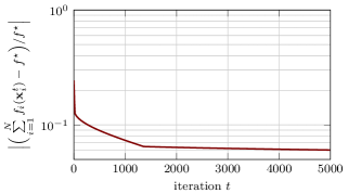
Figure 3: Evolution of the normalized cost error for the basic example.

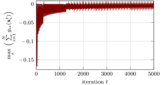
Figure 4: Evolution of the coupling constraint for the basic example. A value below zero means that the solution computed by the algorithm at that iteration is feasible.

VI-B Electric Vehicle Charging Problem

Let us now consider the charging of Plug-in Electric Vehicles (PEVs), which is formulated in detail in [36] and is slightly changed here in order to better highlight the algorithm behavior. The simulations reported in the remainder of this section are all referred to this application scenario.

The problem consists of determining an optimal charging schedule of $N$ electric vehicles. Each vehicle $i$ has an initial state of charge $E_{i}^{\text{init}}$ and a target state of charge $E_{i}^{\text{ref}}$ that must be reached within a time horizon of $8$ hours, divided into $T=12$ time slots of $\Delta T=40$ minutes. Vehicles must further satisfy a coupling constraint, which is given by the fact that the total power drawn from the (shared) electricity grid must not exceed $P^{\text{max}}=N/2$. In this paper, we consider the “charge-only” case. In order to make sure the local constraint set are convex (cf. Assumption II.1), we drop the additional integer constraints considered in [36]. Thus, the vehicles optimize their charging rate rather than activating or de-activating the charging mode at each time slot. Formally, the resulting linear program is

$$\begin{split}\min_{\mathbf{x}_{1},\ldots,\mathbf{x}_{N}}\>&\>\sum_{i=1}^{N}c_{i}^{\top}\mathbf{x}_{i}\\ \textnormal{subj. to}\>&\>\sum_{i=1}^{N}A_{i}\mathbf{x}_{i}\leq b,\\ &\>\mathbf{x}_{i}\in X_{i},\hskip 28.45274pti\in\{1,\ldots,N\},\end{split}$$

where the local constraint sets $X_{i}$ are compact polyhedra and a total of $S=12$ coupling constraints are present. For a complete reference on the other quantities involved in the problem and not explicitly specified here, we refer the reader to the extended formulation in [36].

We consider a network of $N=50$ agents where the underlying graph $\mathcal{E}_{u}$ is generated as an Erdős-Rényi graph with edge probability $0.2$. The edge activation probabilities $\sigma_{ij}$ are randomly picked in $[0.3,0.9]$. In particular, in the next subsections we (i) compare our algorithm with the state of the art, (ii) discuss the parameter $M$ and (iii) show the convergence rate.

VI-C Comparison with State of the Art

We compare DPD-TV with the existing Distributed Dual Subgradient algorithm [10]. As for the algorithm tuning (i.e., the step-size $\alpha^{t}$ in the update (3) and the parameter $M$ appearing in problem (2)), we choose $M=30$ and the diminishing step-size $\alpha^{t}=\frac{1}{(t+1)^{0.6}}$. Our algorithm is initialized in $\mathbf{y}_{i}^{0}=\mathbf{0}$ for all $i$ and the Distributed Dual Subgradient algorithm is initialized in $\boldsymbol{\lambda}_{i}^{0}=\mathbf{0}$ for all $i$. In Figure 5, the cost error of both algorithms is shown, compared with the result of a centralized problem solver. For our algorithm, the symbol $\mathbf{x}_{i}^{t}$ represents the local solution of problem (2) at time $t$, while for the Distributed Dual Subgradient, the same symbol represents the (unweighted) running average of the local solutions over the past iterations. The figure highlights that, in this simulation, DPD-TV reached almost exact cost convergence shortly after $10,000$ iterations with a sudden change of approximately $10$ orders of magnitude. In principle, for the Distributed dual subgradient, it is not possible to have such rapid changes because of the use of running averages.

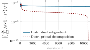
Figure 5: Evolution of the normalized cost error for the comparative study with the state of the art.

In Figure 6, we show the value of the coupling constraints. The picture highlights that both algorithms are able to provide feasible solutions within less than 500 iterations, confirming the primal recovery property.

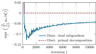
Figure 6: Evolution of the coupling constraint for the comparative study with the state of the art. A value below zero means that the solution computed by the algorithm at that iteration is feasible.

VI-D Impact of the Parameter $M$

We also perform a numerical comparison of the algorithm behavior for different values of the parameter $M$ (see also Section V-B). Under the same set-up of the previous simulation, we use a different initialization to guarantee the requirements imposed by Theorem II.5 and also to create some asymmetry among the initial allocations of the agents. Thus, in this simulation we consider the initialization rule $\mathbf{y}_{i}^{0}=5(N-2i)\mathbf{1}$ for all $i$, which satisfies $\sum_{i=1}^{N}\mathbf{y}_{i}^{0}=\mathbf{0}$.

In Figure 7 we plot the cost error, including the extra penalty term $\sum_{i=1}^{N}M\rho_{i}^{t}$, for three different values of $M$ (all of which satisfy the assumption $M>\|\boldsymbol{\mu}^{\star}\|_{1}$). It can be seen that the slope of the curve decreases as $M$ increases, which agrees with the fact that the larger is $M$, the larger is the set in which subgradients can be found (Lemma IV.3).

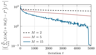
Figure 7: Evolution of the normalized cost error for different values of $M$, under diminishing step-size.

Figure 8 shows the maximum value of $\rho_{i}^{t}$ among agents. Recall that $\rho_{i}^{t}$ is an upper bound on the violation of the local allocation $\mathbf{y}_{i}^{t}$. The picture underlines that such a quantity is forced to zero faster as $M$ gets bigger. This can be intuitively explained by the fact that larger values of the penalty $M\rho_{i}$ drive the algorithm more quickly towards feasibility of the coupling constraint.

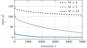
Figure 8: Evolution of the value of $\max_{i}\rho_{i}^{t}$ for varying values of $M$. The quantity represents an upper bound on the coupling constraint violation.

VI-E Numerical Study on Convergence Rates

We finally perform a simulation to point out the different behavior of the algorithm with constant and diminishing step-sizes. Under the same set-up of the previous example, with $M=10$, we run the algorithm with the diminishing step-size law $\alpha^{t}=\frac{0.5}{(t+1)^{0.6}}$ and with the constant step-size $\alpha^{t}=0.01$. As before, agents initialize their local allocation at $\mathbf{y}_{i}^{0}=5(N-2i)\mathbf{1}$ for all $i$.

Figure 9 shows the different algorithm behavior under the two step-size choices. For constant step-size, the algorithm converges within a certain tolerance (which is seen in the picture at around iteration $6,000$), confirming the observations in Section V. Moreover, the sublinear behavior with the diminishing step-size is confirmed. Interestingly, in this example the constant step-size behaved linearly up to iteration $4,000$ and superlinearly in the interval $4,000$–$6,000$, therefore performing much better than the sublinear bound in Proposition V.2.

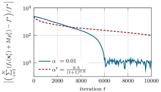
Figure 9: Evolution of the cost error for the comparative study on step-sizes.

VII Conclusions

In this paper, we presented the DPD-TV algorithm to solve constraint-coupled, large-scale, convex optimization problems over random time-varying networks. The proposed algorithm is based on a relaxation and primal decomposition approach, and, for the sake of analysis, it is viewed as an instance of a randomized block subgradient method, in which blocks correspond to edges in the communication graph. Almost sure convergence to the optimal cost of the original problem and an almost sure asymptotic primal recovery property are proved. Sublinear convergence rates are provided under different step-size assumptions. Numerical computations on an electric vehicle charging problem substantiated the theoretical results.

References

- [1] A. Camisa, F. Farina, I. Notarnicola, and G. Notarstefano, “Distributed constraint-coupled optimization over random time-varying graphs via primal decomposition and block subgradient approaches,” in IEEE Conference on Decision and Control, 2019, pp. 6374–6379.
- [2] A. Nedić and A. Ozdaglar, “Distributed subgradient methods for multi-agent optimization,” IEEE Transactions on Automatic Control, vol. 54, no. 1, pp. 48–61, 2009.
- [3] J. C. Duchi, A. Agarwal, and M. J. Wainwright, “Dual averaging for distributed optimization: Convergence analysis and network scaling,” IEEE Transactions on Automatic Control, vol. 57, no. 3, pp. 592–606, 2012.
- [4] M. Zhu and S. Martínez, “On distributed convex optimization under inequality and equality constraints,” IEEE Transactions on Automatic Control, vol. 57, no. 1, pp. 151–164, 2012.
- [5] J. F. Mota, J. M. Xavier, P. M. Aguiar, and M. Püschel, “D-ADMM: A communication-efficient distributed algorithm for separable optimization,” IEEE Transactions on Signal Processing, vol. 61, no. 10, pp. 2718–2723, 2013.
- [6] W. Shi, Q. Ling, K. Yuan, G. Wu, and W. Yin, “On the linear convergence of the ADMM in decentralized consensus optimization,” IEEE Transactions on Signal Processing, vol. 62, no. 7, pp. 1750–1761, 2014.
- [7] D. Jakovetić, J. Xavier, and J. M. Moura, “Fast distributed gradient methods,” IEEE Transactions on Automatic Control, vol. 59, no. 5, pp. 1131–1146, 2014.
- [8] W. Shi, Q. Ling, G. Wu, and W. Yin, “EXTRA: An exact first-order algorithm for decentralized consensus optimization,” SIAM Journal on Optimization, vol. 25, no. 2, pp. 944–966, 2015.
- [9] A. Simonetto and H. Jamali-Rad, “Primal recovery from consensus-based dual decomposition for distributed convex optimization,” Journal of Optimization Theory and Applications, vol. 168, no. 1, pp. 172–197, 2016.
- [10] A. Falsone, K. Margellos, S. Garatti, and M. Prandini, “Dual decomposition for multi-agent distributed optimization with coupling constraints,” Automatica, vol. 84, pp. 149–158, 2017.
- [11] I. Notarnicola and G. Notarstefano, “Constraint-coupled distributed optimization: a relaxation and duality approach,” IEEE Transactions on Control of Network Systems, vol. PP, no. 99, pp. 1–10, 2019.
- [12] T.-H. Chang, A. Nedić, and A. Scaglione, “Distributed constrained optimization by consensus-based primal-dual perturbation method,” IEEE Transactions on Automatic Control, vol. 59, no. 6, pp. 1524–1538, 2014.
- [13] D. Mateos-Núnez and J. Cortés, “Distributed saddle-point subgradient algorithms with laplacian averaging,” IEEE Transactions on Automatic Control, vol. 62, no. 6, pp. 2720–2735, 2017.
- [14] M. Bürger, G. Notarstefano, and F. Allgöwer, “A polyhedral approximation framework for convex and robust distributed optimization,” IEEE Transactions on Automatic Control, vol. 59, no. 2, pp. 384–395, 2014.
- [15] S. Liang, L. Y. Wang, and G. Yin, “Distributed smooth convex optimization with coupled constraints,” IEEE Transactions on Automatic Control, vol. 65, no. 1, pp. 347–353, 2020.
- [16] I. Necoara and V. Nedelcu, “On linear convergence of a distributed dual gradient algorithm for linearly constrained separable convex problems,” Automatica, vol. 55, pp. 209–216, 2015.
- [17] S. Alghunaim, K. Yuan, and A. Sayed, “Dual coupled diffusion for distributed optimization with affine constraints,” in IEEE Conference on Decision and Control, 2018, pp. 829–834.
- [18] T. W. Sherson, R. Heusdens, and W. B. Kleijn, “On the distributed method of multipliers for separable convex optimization problems,” IEEE Transactions on Signal and Information Processing over Networks, vol. 5, no. 3, pp. 495–510, 2019.
- [19] T.-H. Chang, M. Hong, and X. Wang, “Multi-agent distributed optimization via inexact consensus ADMM,” IEEE Transactions on Signal Processing, vol. 63, no. 2, pp. 482–497, 2014.
- [20] Z. Wang and C. J. Ong, “Distributed model predictive control of linear discrete-time systems with local and global constraints,” Automatica, vol. 81, pp. 184–195, 2017.
- [21] R. Carli and M. Dotoli, “Distributed alternating direction method of multipliers for linearly constrained optimization over a network,” IEEE Control Systems Letters, vol. 4, no. 1, pp. 247–252, 2020.
- [22] Y. Zhang and M. M. Zavlanos, “A consensus-based distributed augmented lagrangian method,” in IEEE Conference on Decision and Control, 2018, pp. 1763–1768.
- [23] A. Falsone, I. Notarnicola, G. Notarstefano, and M. Prandini, “Tracking-ADMM for distributed constraint-coupled optimization,” Automatica, vol. 117, p. 108962, 2020.
- [24] A. Beck and L. Tetruashvili, “On the convergence of block coordinate descent type methods,” SIAM Journal on Optimization, vol. 23, no. 4, pp. 2037–2060, 2013.
- [25] M. Razaviyayn, M. Hong, and Z.-Q. Luo, “A unified convergence analysis of block successive minimization methods for nonsmooth optimization,” SIAM Journal on Optimization, vol. 23, no. 2, pp. 1126–1153, 2013.
- [26] P. Richtárik and M. Takáč, “Iteration complexity of randomized block-coordinate descent methods for minimizing a composite function,” Mathematical Programming, vol. 144, no. 1-2, pp. 1–38, 2014.
- [27] C. D. Dang and G. Lan, “Stochastic block mirror descent methods for nonsmooth and stochastic optimization,” SIAM Journal on Optimization, vol. 25, no. 2, pp. 856–881, 2015.
- [28] I. Necoara, “Random coordinate descent algorithms for multi-agent convex optimization over networks,” IEEE Transactions on Automatic Control, vol. 58, no. 8, pp. 2001–2012, 2013.
- [29] I. Necoara, Y. Nesterov, and F. Glineur, “A random coordinate descent method on large-scale optimization problems with linear constraints,” Tech. Rep., 2014.
- [30] D. P. Bertsekas, Nonlinear programming. Athena Scientific, 1999.
- [31] G. J. Silverman, “Primal decomposition of mathematical programs by resource allocation: I – basic theory and a direction-finding procedure,” Operations Research, vol. 20, no. 1, pp. 58–74, 1972.
- [32] A. Camisa, I. Notarnicola, and G. Notarstefano, “A primal decomposition method with suboptimality bounds for distributed mixed-integer linear programming,” in IEEE Conference on Decision and Control, 2018, pp. 3391–3396.
- [33] D. P. Bertsekas, A. Nedić, A. E. Ozdaglar et al., Convex analysis and optimization. Athena Scientific, 2003.
- [34] A. Nedić and A. Ozdaglar, “Approximate primal solutions and rate analysis for dual subgradient methods,” SIAM Journal on Optimization, vol. 19, no. 4, pp. 1757–1780, 2009.
- [35] F. Farina, A. Camisa, A. Testa, I. Notarnicola, and G. Notarstefano, “DISROPT: a Python framework for distributed optimization,” arXiv preprint arXiv:1911.02410, 2019.
- [36] R. Vujanic, P. M. Esfahani, P. J. Goulart, S. Mariéthoz, and M. Morari, “A decomposition method for large scale MILPs, with performance guarantees and a power system application,” Automatica, vol. 67, pp. 144–156, 2016.