Jet transport coefficient $\hat{q}$ in lattice QCD

Abstract

We present the first calculation of the jet transport coefficient $\hat{q}$ in quenched and (2+1)-flavor QCD on a 4-D Euclidean lattice. The light-like propagation of an energetic parton is factorized from the mean square gain in momentum transverse to the direction of propagation, which is expressed in terms of the thermal field-strength field-strength correlator. The leading-twist term in its operator product expansion is calculated on the lattice. Continuum extrapolated quenched results, and full QCD estimates based on un-renormalized lattice data, over multiple lattice sizes, are compared with (non) perturbative calculations and phenomenological extractions of $\hat{q}$ ​​. The lattice data for $\hat{q}$ ​​ show a temperature dependence similar to the entropy density. Within uncertainties, these are consistent with phenomenological extractions, contrary to calculations using perturbation theory.

The study of hot and dense QCD matter, produced in relativistic heavy-ion collisions, using high transverse momentum ($p_{T}$) jets, currently boasts an almost established phenomenology Majumder and Van Leeuwen (2011); Cao and Wang (2020); Burke et al. (2014). The experimental data on various aspects of jet modification is also extensive  Adler et al. (2007); Adare et al. (2010); Adams et al. (2007); Adler et al. (2003); Chatrchyan et al. (2014a); Acharya et al. (2018); Cole (2011); Abelev et al. (2014); Chatrchyan et al. (2014b); CMS-PAS-HIN-11-004 (925220); Aad et al. (2015). Almost all of the evidence points to the formation of a quark-gluon plasma (QGP), a state of matter where the QCD color charge is deconfined over distances larger than the size of a proton Shuryak (1980, 1978). Chiral symmetry – spontaneously broken in a hadron gas – is restored during the transition to the QGP, which is a smooth crossover at zero baryon density centered around the pseudo-critical temperature $T_{pc}=156.5(1.5)$ MeV Bazavov et al. (2019); Borsanyi et al. (2020) (for three physical light quark flavors in the sea). Jets are expected to undergo considerable modification within the QGP compared to confined nuclear matter Gyulassy and Wang (1994).

While a lot of the theoretical development of jet quenching has been focused on modifications to the parton shower, considerably less work has been carried out on the study of the interaction between a parton in the jet with the QGP itself. Most current calculations either model the QGP as a set of slowly moving (or static) heavy scattering centers Gyulassy and Wang (1994); Baier et al. (1995); Wang et al. (1995); Baier et al. (1997a), or in terms of Hard-Thermal Loop (HTL) effective theory Frenkel and Taylor (1990); Braaten and Pisarski (1990a, b); Arnold et al. (2002). Regardless of the model, a description of transverse momentum exchange between the medium and a jet parton can be encapsulated within the transport coefficient Baier (2003)

$$\hat{q}=\frac{\sum_{i=1}^{N_{events}}\sum_{j=1}^{N^{i}(L)}[k_{\perp}^{i,j}]^{2}}{N_{events}\times L}.$$ (1)

The meaning of the above equation is that given a path through a medium with a pre-determined density profile, a single parton may scatter $N^{i}(L)$ times while traversing a distance $L<v\tau_{i}$ in event $i$ ($\tau_{i}$ is the lifetime of the parton which travels at a speed $v$). In each scattering ($j$), it exchanges transverse momentum $k_{\perp}^{i,j}$. In this Letter, we will only focus on momentum exchanges transverse to the direction of the jet parton, as these tend to have a dominant effect on the amount of energy lost via bremsstrahlung from the parton Baier et al. (1997a, b).

In heavy-ion collisions, the density will vary with location, and thus, one necessarily averages over a non-uniform profile, which fluctuates from event to event. Several successful fluid dynamical simulations, which compare to RHIC and LHC data Song et al. (2011); Shen et al. (2011), assuming small density gradients, have used an equation of state calculated in lattice QCD Huovinen and Petreczky (2010) as an input. Unlike the dynamical medium in a heavy-ion collision, lattice simulations assume static media in thermal equilibrium. The use of lattice QCD input in fluid-dynamical simulations is predicated on the ability to reliably coarse grain the system into space-time unit cells, over which intrinsic quantities, e.g., temperature ($T$), entropy density ($s$), pressure ($P$), remain approximately constant.

The calculations in this Letter are an extension of the above principle: Calculations of $\hat{q}$ in the static medium of lattice QCD will be compared with phenomenological estimations, where jets are propagated through a QGP fluid dynamical simulation. These QGP simulations yield the space-time profiles for intrinsic quantities, e.g. $T(\vec{r},t)$, $s(\vec{r},t)$, and $\hat{q}$ is calculated from these, using dimensional parametrization or perturbative techniques. In this Letter, we will compare the dimensionless ratio $\nicefrac{{\hat{q}}}{{T^{3}}}$ between these different approaches Burke et al. (2014).

Following the framework in Ref. Majumder (2013), we consider a jet parton with high energy $E$ and virtuality $Q$ such that $E\!\gg\!Q\!\gg\!\mu_{D}$, the Debye mass in the medium. The choice of a large $E,Q$ leads to a diminished coupling $\alpha_{S}(Q)$ with the medium, due to asymptotic freedom Politzer (1973); Gross and Wilczek (1973). As a result, interactions between the jet parton and a medium of limited extent will be dominated by one-gluon exchange (OGE); i.e. $N^{i}=1$ for all events.

In light-cone coordinates, the incoming quark, traveling in the $-z$ direction, has two non-zero components, $q^{+}=\nicefrac{{(q^{0}+q^{3})}}{{\sqrt{2}}}\ll q^{-}=\nicefrac{{(q^{0}-q^{3})}}{{\sqrt{2}}}$. The quark undergoes a single scattering off the gluon field in the medium and gains transverse momentum $k_{\perp}$ (Fig. 1). In this frame, the momentum of the quark changes from,

$$q_{i}\equiv[q^{+},q^{-},0,0]\rightarrow q_{f}\equiv[q^{+}+\vec{k}_{\perp}^{2}/(2q^{-}),q^{-},\vec{k}_{\perp}].$$ (2)

The matrix element for this process is given as $\mathcal{M}\!=\!\langle q_{f}|\otimes\langle X|\int_{0}^{T_{I}}\!dtd^{3}xg\bar{\psi}(x)\gamma^{\mu}t^{a}A^{a}_{\mu}(x)\psi(x)|n\rangle\otimes|q_{i}\rangle$, where $|n\rangle$ and $|X\rangle$ represent the initial and final state of the medium, respectively. The factors $\psi(x)$, $\bar{\psi}(x)[=\!\psi^{\dagger}\gamma^{0}]$ and $A^{a}_{\mu}(x)$ represent the quark and gluon wave functions (and complex conjugate), with coupling $g$. The spatial integrations are limited within a volume $V=L^{3}$ and the time of interaction ranges from $0$ to $T_{I}=\nicefrac{{L}}{{c}}$ (we use particle physics units with $\hbar,c=1$). Replacing the average over events, with an average over all initial states $|n\rangle$ (energy $E_{n}$) of the medium, weighted by a Boltzmann factor, with $\beta=1/T$ the inverse temperature and $Z$ the partition function of the thermal medium, we obtain,

$$\mbox{}\!\!\!\!\hat{q}=\sum_{n,X}\frac{e^{-\beta E_{n}}}{ZT_{I}}\!\!\int\!\!d^{2}k_{\perp}k_{\perp}^{2}\times\frac{d^{2}W(\vec{k}_{\perp})^{n,X}}{d^{2}k_{\perp}},$$ (3)

where $W^{n,X}\!=\!|\mathcal{M}|^{2}/2N_{C}$ is the scattering probability, for a quark in one of 2 spin and $N_{C}$ color states.

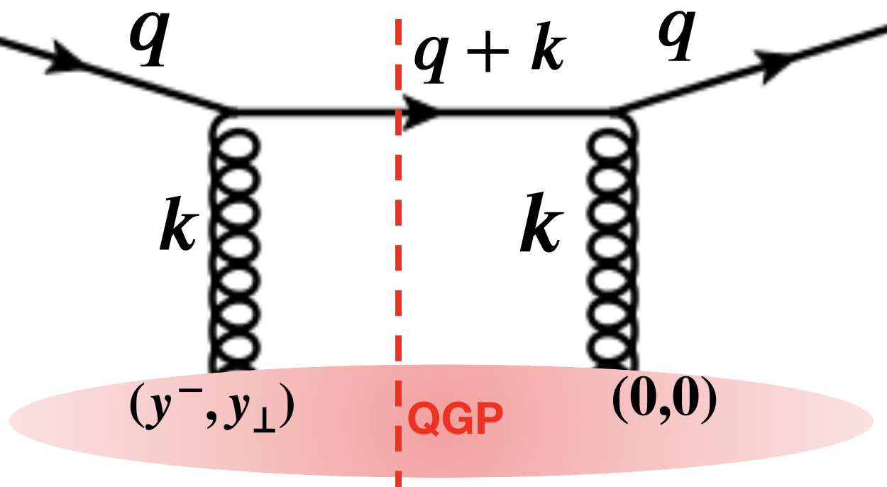
Figure 1: A forward scattering diagram for the hard quark undergoing a single scattering off the gluon field in the plasma. The vertical dashed line represents the cut-line.

Following standard methods outlined in Ref. Majumder (2013), where factors of $k_{\perp}$ are turned into partial derivatives in $y_{\perp}$ and $y^{-}$, we obtain the following well known expression for $\hat{q}$ (assuming $\sum_{X}|X\rangle\langle X|=1$),

$$\hat{q} = c_{0}\int\frac{dy^{-}d^{2}y_{\perp}}{(2\pi)^{3}}d^{2}k_{\perp}e^{-i\frac{\vec{k}^{2}_{\perp}}{2q^{-}}y^{-}+i\vec{k}_{\perp}.\vec{y}_{\perp}}$$ (4)

$$\times \sum_{n}\bra{n}\frac{e^{-\beta E_{n}}}{Z}\mathrm{Tr}[F^{+j}(0)F^{+}_{j}(y^{-},y_{\perp})]\ket{n},$$

where $c_{0}=16\pi\alpha_{s}\sqrt{2}\nicefrac{{C_{R}}}{{(N_{c}^{2}-1)}}$, $C_{R}(=C_{F}$ for a quark) is the representation specific Casimir, $N_{c}$ is the number of colors, $\alpha_{s}$ is the strong coupling constant at the vertex between the hard quark and the glue field, $F^{\mu\nu}=t^{a}F^{a\mu\nu}$ is the bare gauge field-strength tensor. Here and hereafter the index $j=1,2$ runs over transverse directions.

Computing the thermal and vacuum expectation value of the non-perturbative operator $F^{+j}(0)F^{+}_{j}(y^{-},y_{\perp})$ is challenging due to the near light-cone separation between the two field-strength tensors. The separation is slightly space-like $y^{2}=-y_{\perp}^{2}<0$, similar to the case of a parton distribution function (PDF) Ji (2013). Beyond this method, there have been other efforts based on a 3-D Euclidean lattice approach Panero et al. (2014), as well as in classical lattice theory Laine and Rothkopf (2014). Another non-perturbative pure-glue calculation of $\hat{q}$, employed a stochastic vacuum model Antonov and Pirner (2008) with inputs obtained from lattice simulations. However, the current framework remains the sole exploration of $\hat{q}$ in 4-D, first-principles quantum lattice simulations.

To recast $\hat{q}$ in terms of a series of local operators, we apply a method of dispersion as outlined in Ref. Majumder (2013). In this approach, a generalized coefficient is defined as,

$$\begin{split}\mbox{}\!\!\hat{Q}(q^{+})\!=\!c_{0}\!\!\!\int\!\!\frac{d^{4}yd^{4}ke^{iky}}{(2\pi)^{4}}\frac{2q^{-}\langle\mathrm{Tr}[F^{+j}(0)F^{+}_{j}\!(y)]\rangle}{(q+k)^{2}+i\epsilon},\end{split}$$ (5)

where $\langle\dots\rangle\equiv\sum_{n}\bra{n}\ldots\ket{n}e^{-\beta E_{n}}/Z$. The object $\hat{Q}(q^{+})$ has a branch cut in a region where $q^{+}\sim T\ll q^{-}$ corresponding to the quark propagator with momentum $q+k$ going on mass shell (Fig. 1). In this region, the incoming hard quark is light-like, i.e. $q^{2}=2q^{+}q^{-}\approx 0$, and the discontinuity of $\hat{Q}(q^{+})$ is related to the physical $\hat{q}$ as

$$\left.\frac{Disc[\hat{Q}(q^{+})]}{2\pi i}\large\right|_{\hskip 2.84526pt\mathrm{at}\hskip 2.84526ptq^{+}\sim T}=\hat{q}.$$ (6)

In addition to the thermal discontinuity, $\hat{Q}(q^{+})$ also has an additional vacuum discontinuity in the region $q^{+}\in(0,\infty)$ due to real hard gluon emission processes. In this region, the incoming hard quark is time-like. If instead, one takes $q^{+}\ll 0$, e.g. $q^{+}=-q^{-}$, the incoming quark becomes space-like and there is no discontinuity on the real axis of $q^{+}$. In this deep space-like region, the quark propagator can be expanded as follows:

$$\begin{split}\mbox{}\!\!\!\!\!\!\frac{1}{(q+k)^{2}}\!\simeq\!\frac{-1}{\!2q^{-}(q^{-}\!-\!(k^{+}\!-\!k^{-}))}\!=\!\frac{-1}{2(q^{-})^{2}}\!\sum^{\infty}_{n=0}\!\left(\!\!\frac{\sqrt{2}k_{3}}{q^{-}}\!\!\right)^{\!\!n}\!\!\!.\end{split}$$ (7)

Using integration by parts, the factor of exchanged gluon momentum $k_{3}$ [Eq. (7)] is replaced with the regular spatial derivative $\partial_{3}$ acting on the field-strength $F^{+}_{j}(y)$ [Eq. (5)]. A set of higher order contributions from gluon scattering diagrams can be added to promote the regular derivative to a covariant derivative $D_{3}$ (in the adjoint representation). With all factors of $k$ removed from the integrand [Eq. (5)], except for the phase factor, $k$ can be integrated out ($\int d^{4}ke^{iky}$) to yield $\delta^{4}(y)$, setting $y$ to the origin. This yields $\hat{Q}(q^{+}=-q^{-})\,[\equiv\hat{Q}|_{q^{+}=-q^{-}}]$ as,

$$\left.\mbox{}\!\!\!\!\!\!\!\!\hat{Q}\right|_{\mbox{}_{q^{+}=-q^{-}}}\!\!\!\!\!\!\!\!\!\!\!\!\!=c_{0}\langle\mathrm{Tr}[F^{+j}(0)\sum^{\infty}\limits_{n=0}\left(\frac{i\sqrt{2}D_{3}}{q^{-}}\right)^{n}\!\!F^{+}_{j}(0)]\rangle/q^{-};$$ (8)

each term in the series is a local gauge-invariant operator.

To relate $\hat{Q}(q^{+}\!\!=\!\!-q^{-})$ to the physical $\hat{q}$, consider the following contour integral in the $q^{+}$ complex-plane:

$$I_{1}=\oint\frac{dq^{+}}{2\pi i}\frac{\hat{Q}(q^{+})}{(q^{+}+q^{-})}=\hat{Q}(q^{+}=-q^{-}),$$ (9)

where the contour is taken as a small anti-clockwise circle centered around point $q^{+}\!\!=\!\!-q^{-}$, with a radius small enough to exclude regions where $\hat{Q}(q^{+})$ may have discontinuities. Alternatively, the integral can be evaluated by analytically deforming the contour over the branch cut of $\hat{Q}(q^{+})$ for $q^{+}\in(-T_{1},\infty)$ and obtaining Eq. (9) as:

$$\begin{split}\mbox{}\!\!\!\!\hat{Q}(q^{\!+}\!\!=\!-q^{\!-\!})\!=\!\!\!\!\int\limits^{T_{2}}_{-T_{1}}\!\!\!\frac{dq^{+}}{2\pi i}\frac{\!Disc[\hat{Q}(\!q^{+}\!)]\!}{\!(q^{+}\!+q^{-})}\!+\!\!\int\limits^{\infty}_{0}\!\frac{\!dq^{\!+}}{\!2\pi i\!}\frac{Disc[\hat{Q}(q^{+}\!)]}{(q^{+}\!+q^{-})}.\end{split}\!\!\!$$ (10)

The limits $-T_{1}$ and $T_{2}$ in the first integral represent lower and upper bounds of $q^{+}[=k^{+}\!\!+\nicefrac{{k_{\perp}^{2}}}{{(2q^{-}\!\!+2k^{-})}}]$, beyond which the thermal discontinuity in $\hat{Q}(q^{+})$ on the real axis of $q^{+}$ is zero. In this region, the hard incoming quark is close to on-shell, i.e. $q^{2}=2q^{+}q^{-}\approx 0$ and undergoes scattering with the medium. The second integral in Eq. (10) corresponds to the contributions from vacuum-like processes, where the time-like hard quark with momentum $q^{+}\in(0,\infty)$ undergoes vacuum-like splitting. Hence, the second integral is temperature independent.

Using Eqs. (6-10), we obtain (suppressing $y^{-}\!=\!y_{\perp}\!=\!0$),

$$\mbox{}\!\!\!\!\frac{\hat{q}}{T^{3}}=\frac{c_{0}\!\!\sum\limits^{\infty}_{n=0}\!\left(\!\frac{T}{q^{-}}\!\right)^{\!\!2n}\!\!\!\left\langle\!\!\frac{1}{T^{4}}\mathrm{Tr}\left[F^{+j}\Delta^{2n}\!F^{+}_{j}\!\right]\!\right\rangle_{(\mathrm{T-V})}}{\nicefrac{{(T_{1}+T_{2})}}{{T}}},$$ (11)

where the subscript $(\mathrm{T-V})$ represents the vacuum subtracted expectation value and $T_{1}+T_{2}\simeq 2\sqrt{2}T$ represents a width of the thermal discontinuity of $\hat{Q}(q^{+})$. We abbreviate the differential operator as $\Delta\equiv\nicefrac{{i\sqrt{2}D_{3}}}{{T}}$. The above expression for the transport coefficient $\hat{q}$ contains several features: Each term in the series is local, allowing for their computation on the lattice. The successive terms in the series are suppressed by the hard scale $q^{-}$, and hence, computing only the first few terms will be sufficient . The expression for $\hat{q}$ given in Eq. (11) applies after appropriate renormalization of the coupling and the field strength operators , for the hard quark traversing either the pure glue plasma, or a QGP. While the field strength operators mix in QCD with corresponding sea quark operators , the latter do not contribute in Eq. (11), besides this mixing.

To compute the operators on the lattice, we perform Wick rotation $x^{0}\!\rightarrow\!-ix^{4},A^{0}\!\rightarrow\!iA^{4}\!\Longrightarrow\!F^{0j}\!\rightarrow\!iF^{4j}$. We have studied the first three non-zero operators in the $\hat{q}$ series , $\hat{O}_{n}=\nicefrac{{\mathrm{Tr}[F_{3j}\Delta^{2n}F_{3j}\!-\!F_{4j}\Delta^{2n}F_{4j}]}}{{T^{4}}}$  (summed over $j$; $n=0,1,2$). The $F_{\mu\nu}$ is discretized via clover-leaf operators projected to anti-Hermitian traceless matrices,

$$\mbox{}\!\!\!\!\!ig_{0}\mathcal{F}_{\mu\nu}(x) = \frac{\mathcal{P}Q_{\mu\nu}(x)}{a_{L}^{2}}=ig_{0}F_{\mu\nu}+\mathcal{O}(a_{L}^{2})$$ (12)

with $Q_{\mu\nu}=\nicefrac{{[U_{\mu,\nu}+U_{\nu,-\mu}+U_{-\mu,-\nu}+U_{-\nu,\mu}]}}{{4}}$ ($U_{\mu,\nu}$ being the plaquette) and $\mathcal{P}Q=(Q-Q^{\dagger}-\nicefrac{{\mathrm{Tr}[Q-Q^{\dagger}]}}{{N_{c}}})/2$. We note that the bare leading-twist operator stripped of its prefactor $\nicefrac{{c_{0}T}}{{(T_{1}+T_{2})}}$ (hereafter: $\hat{O}_{0}\equiv\nicefrac{{FF}}{{T^{4}}}$) [Eq. (11)] coincides in imaginary time up to a trivial algebraic factor $T_{F}=\nicefrac{{1}}{{2}}$ with the bare gluon contribution to the scaled entropy density $\nicefrac{{s}}{{T^{3}}}$ (via clover-leaf operator). The higher-twist contributions ($n\!>\!0$) turn out to be negligible in the limit of very large jet energy ($q^{-}\rightarrow\infty$), and are only discussed in the Supplemental Material Sup .

We have generated $T\!>\!0$ lattices with aspect ratio $\nicefrac{{n_{\sigma}\!}}{{n_{\tau}}}\!\!=\!4$ for $n_{\tau}\!\!=\!4,6$ and $8$ [$T\!\!=\!\nicefrac{{1}}{{(a_{L}n_{\tau})}}$], and also corresponding $T\!\!=\!0$ lattices with $n_{\tau}\!\!=\!\!n_{\sigma}$ using the MILC code MIL (2017) and the USQCD software stack Sci . We use the Rational Hybrid Monte Carlo algorithm Clark et al. (2005) with highly improved staggered quark (HISQ) action Follana et al. (2007) and tree-level Symanzik gauge action Bazavov et al. (2014, 2018a) for (2+1)-flavor QCD. The leading cutoff effects are $\mathcal{O}(a^{4})$ and $\mathcal{O}(g^{2}_{0}a^{2})$. We employ tuned input parameters (bare lattice coupling $\beta_{0}=10/g_{0}^{2}$, and bare quark masses), and use the $r_{1}$ lattice scale following Refs. Bazavov et al. (2014, 2016, 2018b, 2018a) by the HotQCD and TUMQCD collaborations. This setup has a physical strange and two degenerate light quarks with $m_{l}=m_{s}/20$ corresponding to a pion mass of about 160 MeV in the continuum limit. We have generated pure gauge ensembles via the heat-bath algorithm using Wilson gauge action Wilson (1974) with $\beta_{0}\!=\!6/g^{2}_{0}$ and leading cutoff effects $\mathcal{O}(a^{2})$. (See Supplemental Material for details about the gauge ensembles Sup ).

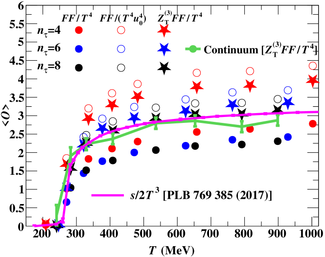
Figure 2: Bare and renormalized leading-twist operator $\langle\mathrm{T}r[F^{3i}F^{3i}\!-\!F^{4i}F^{4i}]\rangle/T^{4}$ in pure SU(3) gauge theory. Our result agrees with the entropy density obtained in shifted boundary condition approach Giusti and Pepe (2017) after rescaling by $T_{F}=\nicefrac{{1}}{{2}}$.

Using published data Giusti and Pepe (2015) we renormalize (in $\overline{MS}$ Capitani (2003)) $\nicefrac{{FF}}{{T^{4}}}$ in pure gauge theory by converting the sextet renormalization factor $Z_{T}^{(6)}(g_{0}^{2})$ Giusti and Pepe (2017) (clover-leaf) to triplet via $Z_{T}^{(3)}(g_{0}^{2})=z_{T}(g_{0}^{2})Z_{T}^{(6)}(g_{0}^{2})$ Giusti and Pepe (2015). We interpolate $\nicefrac{{Z_{T}^{(3)}FF}}{{T^{4}}}$ on the coarser ensembles ($n_{\tau}\leq 6$) linearly to the temperatures of the finest ensemble ($n_{\tau}=8$), and then extrapolate at each temperature the two finest ensembles linearly [$\propto\nicefrac{{1}}{{n_{\tau}^{2}}}$] or all three ensembles with a further quadratic term [$\propto\nicefrac{{1}}{{n_{\tau}^{4}}}$] to the continuum. The linear fit provides the central value and the statistical error, while the spread between the central value from the linear fit and the quadratic fit give us the systematic error. Both the errors are added in quadrature and shown in green vertical bar in Fig. 2. Our results agree with the $T_{F}$-rescaled entropy density using the shifted boundary condition approach Giusti and Pepe (2017), while estimating $Z^{(3)}_{T}(g_{0}^{2})$ as $\nicefrac{{1}}{{u_{0}^{4}(g_{0}^{2})}}$ – with tadpole factor $u_{0}(g_{0}^{2})=\sqrt[4]{\nicefrac{{\langle\mathrm{Tr}[U_{\mu,\nu}]\rangle}}{{N_{c}}}}$ – yields roughly 10% higher values (Fig. 2).

In Fig. 3 we present the resulting $\hat{q}/T^{3}$ based on Eq. (11). The coupling at the vertex to gluons absorbed by the medium must be at the temperature scale. We vary this scale as $(2-4)\pi T$ to account for the truncation error and use of the 1-loop gauge coupling. While the non-perturbative renormalization factors for the (2+1)-flavor QCD result are unknown, we have used several means to obtain well-justified estimates. In pure gauge, the tadpole factor yields a 10% shift from the renormalized result. Also the bare $\nicefrac{{FF}}{{T^{4}}}$ for $n_{\tau}\!\!=\!6$ is about 10% higher than the $n_{\tau}\!\!=\!8$ due to cutoff effects (similar trend for $\nicefrac{{Z_{T}^{(3)}FF}}{{T^{4}}}$, when comparing to the continuum limit) in pure gauge. Based on 1-loop considerations, we estimate that mixing with quark operators, not accounted for, maybe at most an effect of commensurate size; see Supplemental Material for an extended discussion of these arguments, and complementary considerations relying on similarity of the nonperturbative entropy density and weak-coupling results Sup . As we expect a deviation of no more than 30% (adding all three sources of systematic uncertainty) between $FF/(T^{4}u^{4}_{0})$ [$n_{\tau}\!\!=\!6$] and the correctly renormalized continuum limit, we attach a symmetric relative uncertainty of 30% to this lattice QCD estimate. We multiply by the 1-loop gauge coupling (same scale variation) for $N_{f}=3$.

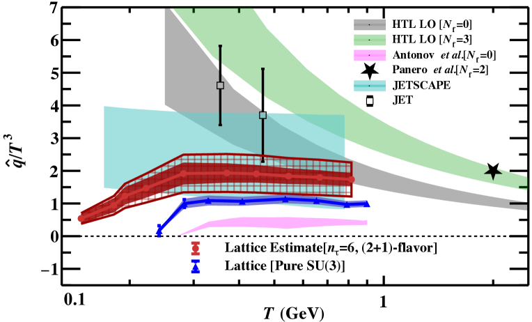
Figure 3: Lattice determination of $\hat{q}$ for a highly energetic hard quark traversing a pure glue (blue) and (2+1)-flavor QCD (red) plasma. Error bars show statistical errors, solid bands represent scale variation. The pure SU(3) result is renormalized and continuum extrapolated. For the QCD estimate, systematic errors due to estimated renormalization (via $u_{0}$) and lattice cutoff ($n_{\tau}\!=\!6$) are indicated by the checkered band. Also plotted are the phenomenological extractions from the JET Burke et al. (2014) and JETSCAPE Soltz (2019) collaborations, non-perturbative results from an $N_{f}\!=\!2$, 3-D lattice calculation Panero et al. (2014), an $N_{f}\!=\!0$ stochastic vacuum model calculation Antonov and Pirner (2008), and LO-HTL calculations from Ref. He et al. (2015), with $\alpha_{S}$ evaluated at $2\pi T\leq\mu\leq 4\pi T$.

Due to the OGE approximation [Eqs. (3),(4)], truncation at leading twist [Eq. (11)], and the coupling $g(T)$ at the temperature scale, $q^{-}$ dependence is absent in our result for $\nicefrac{{\hat{q}}}{{T^{3}}}$. Hence, this result applies in the limit $q^{-}\to\infty$ of an infinitely hard parton. The temperature dependence of the resulting $\nicefrac{{\hat{q}}}{{T^{3}}}$ is shown in Fig. 3 for the continuum limit of pure SU(3) gauge theory (blue) or for our estimate in (2+1)-flavor lattice QCD (red).

The transport coefficient $\nicefrac{{\hat{q}}}{{T^{3}}}$ exhibits a rapid rise in the transition region and slightly above, i.e. in the temperature range $150\,\mathrm{MeV}\!\lesssim\!T\!\lesssim\!250\,\mathrm{MeV}$ for (2+1)-flavor QCD or $250\,\mathrm{MeV}\!\lesssim\!T\!\lesssim\!350\,\mathrm{MeV}$ for the pure SU(3) gauge theory, and is flat within errors above $400\,\mathrm{MeV}$. The change of the gauge coupling $g(T)$ with $T$ partially compensates the temperature dependence of the leading-twist operator at temperatures well above $T_{pc}$. Interestingly, the nonperturbative stochastic vacuum model result Antonov and Pirner (2008) exhibits a very similar behavior.

Expectedly, the lattice results do not show any log-like rise at lower $T$, as one observes in leading-order (LO) HTL calculations Qin and Majumder (2010) (for the HTL bands in Fig. 3 $q^{-}\!\!=\!100$ GeV is assumed). This arises from the dominant diagram with OGE in the perturbative calculation, which leads to a logarithm in $q^{-}/T$. Interestingly, no such logarithm arises at next-to-leading-order (NLO) in the HTL expansion of $\hat{q}$ Caron-Huot (2009). The finite part of the NLO result is much larger than the LO result and far above the scale in Fig. 3. Similar contributions may appear once some approximations used in this paper are lifted, e.g. if emission of gluons is considered, or if the higher-twist operators become non-negligible as $q^{-}\!\to\!\infty$ is relaxed. Whether such terms will dominate remains to be determined. The 3-D lattice simulation Panero et al. (2014) exhibits a behavior quite similar to perturbative HTL; the result at $T=400\,\mathrm{MeV}$ is far above the scale in Fig. 3.

In Fig. 3, we also present a comparison with phenomenological extractions of $\nicefrac{{\hat{q}}}{{T^{3}}}$ obtained by the JET Burke et al. (2014) and JETSCAPE Soltz (2019) collaborations. The JET collaboration applied several disparate models of energy loss with either a sole $T$ dependence of the ratio $\nicefrac{{\hat{q}}}{{T^{3}}}$, or one obtained from HTL effective theory Caron-Huot (2009). The JETSCAPE extraction applied an amalgam of theories for different epochs of the jet shower, with a data-driven (Bayesian) determination of $\nicefrac{{\hat{q}}}{{T^{3}}}$, allowed to depend on $T$, the energy and scale of a given parton in the shower. A log-like rise at low $T$ is allowed in both frameworks; both work with the OGE approximation.

In this Letter, we carried out the first rigorous first-principles 4-D calculation of the jet quenching parameter $\hat{q}$, which is the leading coefficient affecting jet modification in the QGP. We computed $\hat{q}$ for a single parton undergoing a single scattering off the medium, utilizing lattice gauge theory in the quenched approximation. We outlined the specific challenges of a corresponding (2+1)-flavor lattice calculation, while providing a first theoretically motivated lattice estimate of $\hat{q}$ in (2+1)-flavor QCD.

While the proximity of the lattice calculations with phenomenological extractions is very encouraging, several caveats need to be considered: The full QCD result is only an estimate, due to lack of rigorous control of the renormalization factors and the mixing with still unknown quark operators on the lattice.

As the $q^{-}\to\infty$ limit is relaxed, the perturbative portions of the current calculation will have to be extended to higher-order, allowing for multiple scattering and emission in the medium. While we do not expect multiple scattering to yield contributions that cannot be factorized into independent scatterings (as is the case in all pQCD based jet quenching calculations and phenomenology, including the extractions from the JET and JETSCAPE collaborations), emissions in the process of scattering may lead to shifts (in $\nicefrac{{\hat{q}}}{{T^{3}}}$) of the order of the width of the bands in our QCD estimates. As discussed in the Supplemental Material section Sup , applying known perturbatively calculated renormalization factors Blaizot et al. (2013); Blaizot and Mehtar-Tani (2014); Liou et al. (2013), will bring down the phenomenological extractions by about 33%, dramatically increasing the agreement with our calculations. Future efforts which expand Eq. (11) as a power series in $\nicefrac{{T}}{{q^{-}}}$, will encounter mixings with novel quark operators at order $\nicefrac{{T}}{{q^{-}}}$. At order $(\nicefrac{{T}}{{q^{-}}})^{2}$, one will encounter mixing with possible linearly divergent, temperature dependent operators, that cannot be straightforwardly canceled via vacuum subtraction (see Supplemental Material).

Acknowledgements. We thank A. Patella, R. Sommer, and M. Dalla Brida for extensive discussion about the renormalization of the EMT. This work was supported in part by the National Science Foundation (NSF) under grant number ACI-1550300 (JETSCAPE), by the U.S. Department of Energy (DOE) under grant number DE-SC0013460. JHW’s research is funded by the Deutsche Forschungsgemeinschaft (DFG, German Research Foundation) - Projektnummer 417533893/GRK2575 “Rethinking Quantum Field Theory”.

Appendix A Supplemental Material for “Jet transport coefficient $\hat{q}$ in lattice QCD”

A.1 Gauge ensembles and lattice setup

In this document, we list the parameters used in generating gauge ensembles for pure SU(3) and (2+1)-flavor QCD lattices. In the presented lattice calculations, the unquenched lattices were generated at the physical value of the strange quark mass $m_{s}$ and the light sea quark masses of $m_{l}=m_{s}/20$ using the HISQ Follana et al. (2007) and tree-level Symanzik improved gauge action Bazavov et al. (2014, 2018a). We employed the Rational Hybrid Monte Carlo algorithm (RHMC) Clark et al. (2005). In Table 1, 2 and 3, we present the strange quark mass ($am_{s}$) in units of lattice spacing $a$, temperature ($T$) and time units (TU) for $n_{\tau}=4,6,8$ and their vacuum analog $T=0$. The temperatures for different $\beta_{0}=10/g^{2}_{0}$’s have been fixed using the $r_{1}$ scale and taken from Refs. Bazavov et al. (2018a).

$\beta_{0}=10/g^{2}_{0}$	$am_{s}$	$T$ (MeV)	$\#$TUs($T$$\neq$0)	$\#$TUs($T$=0)
5.9	0.132	201	10000	10000
6.0	0.1138	221	10000	10000
6.285	0.079	291	10000	10000
6.515	0.0603	364	10000	10000
6.664	0.0514	421	20000	10000
6.95	0.0386	554	10000	10000
7.15	0.032	669	10000	10000
7.373	0.025	819	10000	10000

Table 1: The parameters to generate (2+1)-flavor QCD gauge ensembles with $m_{l}=m_{s}/20$ for lattice size $n_{\tau}=4$ with aspect ratio $n_{s}/n_{\tau}=4$ .

$\beta_{0}=10/g^{2}_{0}$	$am_{s}$	$T$ (MeV)	$\#$TUs($T$$\neq$0)	$\#$TUs($T$=0)
6.0	0.1138	147	10000	10000
6.215	0.0862	181	10000	10000
6.285	0.079	194	10000	10000
6.423	0.067	222	7600	10000
6.664	0.0514	281	10000	7000
6.95	0.0386	370	10000	8000
7.15	0.032	446	10000	8600
7.373	0.025	547	10000	10000
7.596	0.0202	667	8600	10000
7.825	0.0164	815	9140	10000

Table 2: The parameters to generate (2+1)-flavor QCD gauge ensembles with $m_{l}=m_{s}/20$ for lattice size $n_{\tau}=6$ with aspect ratio $n_{s}/n_{\tau}=4$ .

In Table 4, 5 and 6, we provide $\beta_{0}$, temperature and the collected statistics for pure SU(3) lattices. The scale setting was done using the two-loop perturbative renormalization group (RG) equation with non-perturbative correction factor [$f(\beta_{0})$] given as

$$a=\frac{f(\beta_{0})}{\Lambda_{L}}\left[\frac{11g^{2}_{0}}{16\pi^{2}}\right]^{\frac{-51}{121}}\exp\left[\frac{-8\pi^{2}}{11g^{2}_{0}}\right]$$ (1)

where $\Lambda_{L}$ is a lattice parameter. We estimated the non-perturbative factor by adjusting the function $f(\beta_{0})$ such that $T_{c}/\Lambda_{L}$ is independent of bare coupling constant $g_{0}$. In this calculation, $\Lambda_{L}$ was set $5.5$ MeV Hasenfratz and Hasenfratz (1980); Booth et al. (2001); Deur et al. (2016) and the critical temperature to $T_{c}\approx 265$ MeV Philipsen (2013).

$\beta_{0}=10/g^{2}_{0}$	$am_{s}$	$T$ (MeV)	$\#$TUs($T$$\neq$0)	$\#$TUs($T$=0)
6.515	0.0604	182	7300	6400
6.575	0.0564	193	8650	6800
6.664	0.0514	211	10000	5000
6.95	0.0386	277	10000	5950
7.28	0.0284	377	10000	6550
7.5	0.0222	459	10000	5000
7.596	0.0202	500	10000	9400
7.825	0.0164	611	10000	7900
8.2	0.01167	843	10000	5000

Table 3: The parameters to generate (2+1)-flavor QCD gauge ensembles with $m_{l}=m_{s}/20$ for lattice size $n_{\tau}=8$ with aspect ratio $n_{s}/n_{\tau}=4$ .

$\beta_{0}=6/g^{2}_{0}$	$T$ (MeV)	$\#$TUs($T$$\neq$0)	$\#$TUs($T$=0)
5.6	209	10000	10000
5.7	271	10000	10000
5.8	336	10000	10000
5.9	406	10000	10000
6.0	482	10000	10000
6.2	658	10000	10000
6.35	816	10000	10000
6.5	1003	10000	10000
6.6	1146	10000	10000

Table 4: The parameters to generate pure SU(3) gauge ensembles using Wilson’s pure SU(3) gauge action for lattice size $n_{\tau}=4$ with aspect ratio $n_{s}/n_{\tau}=4$ .

$\beta_{0}=6/g^{2}_{0}$	$T$ (MeV)	$\#$TUs($T$$\neq$0)	$\#$TUs($T$=0)
5.60	139	10000	10000
5.85	247	10000	10000
5.90	271	10000	10000
6.00	321	10000	10000
6.10	377	10000	10000
6.25	472	10000	10000
6.45	625	10000	10000
6.60	764	10000	10000
6.75	929	10000	10000
6.85	1056	10000	10000

Table 5: The parameters to generate pure SU(3) gauge ensembles using Wilson’s pure SU(3) gauge action for lattice size $n_{\tau}=6$ with aspect ratio $n_{s}/n_{\tau}=4$ .

$\beta_{0}=6/g^{2}_{0}$	$T$ (MeV)	$\#$TUs($T$$\neq$0)	$\#$TUs($T$=0)
5.70	135	10000	10000
5.95	221	10000	10000
6.00	241	10000	10000
6.10	283	10000	10000
6.20	329	10000	10000
6.35	408	10000	10000
6.55	536	10000	10000
6.70	653	10000	10000
6.85	792	10000	10000
6.95	899	10000	10000

Table 6: The parameters to generate pure SU(3) gauge ensembles using Wilson’s pure SU(3) gauge action for lattice size $n_{\tau}=8$ with aspect ratio $n_{s}/n_{\tau}=4$ .

A.2 Temperature dependence of bare operators

We present the expectation values of the bare field strength operators $\hat{O}_{n}$ in Fig. 4 for all ensembles ($n_{\tau}=8,~{}6$ and $4$) in pure gauge theory or (2+1)-flavor QCD. The operators $\hat{O}_{n}=\nicefrac{{\mathrm{Tr}[F_{3j}\Delta^{2n}F_{3j}\!-\!F_{4j}\Delta^{2n}F_{4j}]}}{{T^{4}}}$  (summed over $j$; $n=0,1,2$), respectively, where $\Delta\equiv\nicefrac{{i\sqrt{2}D_{3}}}{{T}}$. The vacuum contributions have been subtracted while computing the temperature dependence; for the leading-twist operator, $\hat{O}_{0}$, the vacuum contribution vanishes within the statistical error as naively expected (In the one gluon exchange approximation, the vacuum contribution corresponds to the difference of the transverse electric and magnetic field squared of a radiated on-shell gluon, which is identically zero). The operator $\hat{O}_{0}$ exhibits a rapid transition near the temperature $T\in(150,250)$ MeV for full QCD case and $T\in(250,350)$ MeV for pure SU(3) gauge theory. The operators with derivatives $\Delta$ are scaled by the factor $10^{-4}$ and $10^{-8}$ to illustrate the ordering of operators as an overall factor of $(T/q^{-})^{2n}$ appears in $\hat{q}$ expression Eq. (11); it corresponds to a hard parton, i.e. $T\sim 1$ GeV and $q^{-}\sim 100$ GeV. Looking at the operators $\hat{O}_{1}$ and $\hat{O}_{2}$ for pure SU(3) case where the statistics of the $T=0$ ensembles is much better, one observes an upward movement of data points as one goes from coarser to finer lattices, i.e. from $n_{\tau}=4$ to $n_{\tau}$=8 (note the log-scale). This enhancement might be indicative of a divergence due to mixing with lower-dimensional operators. Both higher-twist operators also increase as the temperature is reduced; however, once the powers of temperature in the prefactors are taken into account, $T^{2}\hat{O}_{1}$ and $T^{4}\hat{O}_{2}$ decrease instead. Whether the bump at low temperatures could be a signature of sensitivity to critical behaviour near the transition region is an open question. The full QCD result exhibits a similar pattern, albeit with large errors for $n_{\tau}=8$. Since we have not worked out the mixing of $\hat{O}_{1}$ and $\hat{O}_{2}$ operators with the respective lower dimensional operators, we shall estimate $\hat{q}$ in the limit of the hard parton energy $q^{-}\rightarrow\infty$, where the higher-twist terms do not contribute at all.

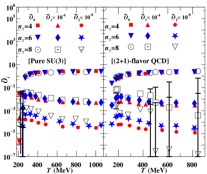
Figure 4: Temperature dependence of vacuum-subtracted field-strength correlators on quenched and unquenched SU(3) lattices. The operators are unrenormalized and have been computed for lattice sizes $n_{\tau}=4,6$ and $8$.

A.3 Renormalization of leading-twist operator in full QCD

As mentioned in the main body of the paper, the calculation of $\hat{q}$ is substantially more involved in QCD than in pure gauge theory. In pure gauge theory, on the one hand, the renormalized leading-twist operator $\nicefrac{{FF}}{{T^{4}}}\equiv\nicefrac{{\mathrm{Tr}[F_{3j}F_{3j}-F_{4j}F_{4j}]}}{{T^{4}}}$ is a genuine observable and trivially related to the renormalized energy-momentum tensor (EMT), here in the triplet representation $T^{(3)}$ . The same relation holds for the bare variables: $FF\equiv[FF]^{B}=T_{F}T^{(3)B}$ (with $T_{F}=\nicefrac{{1}}{{2}}$). Both undergo multiplicative renormalization with a (finite) factor $Z^{(3)}_{T}$ fixed by finite-momentum Ward identities, i.e. $T^{(3)R}=Z^{(3)}_{T}T^{(3)B}$ and $[FF]^{R}=Z^{(3)}_{T}[FF]^{B}$. While $Z^{(3)}_{T}=1$ is trivial in the continuum theory, it explicitly depends on the particular discretization of the gauge field operator (in our case, a separate clover-leaf operator for each field strength tensor) and of the lattice gauge action that determines the background gauge field. In the rest frame, the EMT’s triplet component coincides with the entropy density times the temperature, $T^{(3)R}=sT$, underscoring the status of $[FF]^{R}$ as a scheme-independent observable in the pure gauge theory. In QCD, on the other hand, the leading-twist operator is not scheme-independent, and the previous relation to the entropy density $s$ does not hold. Instead, the renormalized leading-twist operator satisfies $[FF]^{R}=T_{F}T^{(3)R}_{G}$, i.e. only the renormalized gauge field operator’s contribution to the EMT is considered, while the gauge background and higher order terms contain explicit contributions from the quark sea. The full entropy density $s$ is indeed a scheme-independent observable, and its renormalization is fixed by finite-momentum Ward identities, i.e. $sT=T^{(3)R}_{G+Q}=Z^{(3)}_{G}T^{(3)B}_{G}+Z^{(3)}_{Q}T^{(3)B}_{Q}$ in the rest frame. Both $Z^{(3)}_{G}$ and $Z^{(3)}_{Q}$ are finite, and can be fixed by two different finite momentum Ward identities using two different values of imaginary chemical potential. Here, $T^{(3)B}_{G}=[FF]^{B}$ is the same bare gauge field operator as in pure gauge theory (but on a QCD background), while $T^{(3)B}_{Q}$ is its valence quark counterpart ($N_{f}$ explicit contributions, i.e. from each of the sea quarks). We note that the choice of the regularization of $T^{(3)B}_{Q}$ does not have to coincide with the choice of the quark action of the QCD background fields. In lattice-regularized QCD, the renormalized gauge field and quark operators are related to the bare ones by a mixing matrix $\mathcal{Z}$ as

$$\left(\begin{array}[]{c}T^{(3)R}_{G}\\ T^{(3)R}_{Q}\end{array}\right)=\mathcal{Z}\left(\begin{array}[]{c}T^{(3)B}_{G}\\ T^{(3)B}_{Q}\end{array}\right),\quad\mathcal{Z}\equiv\left(\begin{array}[]{cc}\mathcal{Z}^{(3)}_{GG}&\mathcal{Z}^{(3)}_{GQ}\\ \mathcal{Z}^{(3)}_{QG}&\mathcal{Z}^{(3)}_{QQ}\end{array}\right)$$ (2)

where $\mathcal{Z}^{(3)}_{GG}\equiv Z^{(3)}_{G}+z_{G}$ and $\mathcal{Z}^{(3)}_{QQ}\equiv Z^{(3)}_{Q}+z_{Q}$. The off-diagonal components $\mathcal{Z}^{(3)}_{GQ}\equiv-z_{Q}$ or $\mathcal{Z}^{(3)}_{QG}\equiv-z_{G}$ diverge as the regulator is removed, and so do the bare operators. Moreover, the coefficients $z_{G,Q}$ cannot be fixed using Ward identities, such that additional renormalization conditions need to be chosen to fix these in some particular scheme. Hence, $T^{(3)R}_{G}$ (and $T^{(3)R}_{Q}$) are renormalization scheme dependent in QCD. Without such a scheme being fixed before the regulator is removed, or without including the bare quark operator $T^{(3)B}_{Q}$, $T^{(3)R}_{G}$ and its continuum limit cannot be defined in QCD at all. For our lattice setup in QCD, neither the renormalization factors are known, nor the bare quark operators have been computed.

For these reasons we currently can only produce an estimate of the renormalized leading-twist operator $[FF]^{R}$ for (2+1)-flavor QCD based on various complementary arguments. The first set of such considerations are of a purely quantitative nature, and concern reasonable estimates of the non-perturbative renormalization factors and cutoff effects in pure gauge theory that are transferred to the full QCD case. They have been discussed in the main body of the Letter and will not be repeated.

The second set of considerations relies on properties of the equation of state. The nonperturbative entropy density $s(T)$ or pressure $P(T)$ Bazavov et al. (2018b); Weber et al. (2019) are about 30% below the Stefan-Boltzmann limit at $T\sim 2\,T_{pc}$, with the deviation diminishing by almost half at $T\sim 1$ GeV. For these and higher temperatures, the nonperturbative results are bracketed by electrostatic QCD (EQCD) at $\mathcal{O}(g^{6})$ Laine and Schroder (2006) and HTL-resummed perturbation theory at 3-loop order Haque et al. (2014) with less than 10% deviation. This justifies assuming that the relative size of the (renormalized) gluon fraction of the full nonperturbative result can be estimated in the weak-coupling limit, i.e. the gluon fraction of $s(T)$ (and thus $T^{(3)}$) in (2+1)-flavor QCD being approximately $R_{\mathrm{SB}}~{}=~{}\nicefrac{{32}}{{95}}\approx 0.337$ (of the SB limit). Thus, scaling down $T_{F}sT$ by this factor we may arrive at a QCD estimate of the renormalized leading-twist operator $[FF]^{R}$ that is quantitatively similar to the previous estimate. The aforementioned spread of up to 30% between nonperturbative result and the SB limit appears to be a fairly cautious estimate of the uncertainty associated with this estimate of $[FF]^{R}$ for $T\gtrsim 2\,T_{pc}$. Defining the ratio $R_{\mathrm{EQCD}}(\nicefrac{{T}}{{T_{pc}}})$ between the $N_{f}=0$ to $N_{f}=3$ EQCD results at $\mathcal{O}(g^{6})$ and fixed value of $\nicefrac{{T}}{{T_{pc}}}$, and rescaling the (2+1)-flavor QCD lattice result is expected to be an even better estimate, since the EQCD results are even more similar to the lattice data. In Fig. 5 we show that both estimates of the gluon fraction of the entropy density in full QCD yield similar results that are within the 30% uncertainty margin, and confirm the expectation of a downward correction for the continuum limit.

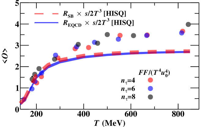
Figure 5: Comparison of the tadpole-factor rescaled leading-twist operator $\langle\mathrm{Tr}[F^{3j}F^{3j}-F^{4j}F^{4j}]/(T^{4}u^{4}_{0})\rangle$ with $T_{F}$-rescaled entropy $\nicefrac{{s}}{{T^{3}}}$ in (2+1)-flavor QCD Bazavov et al. (2018b); Weber et al. (2019) scaled by the gluon fraction in the Stefan-Boltzmann limit ($R_{\mathrm{SB}}$) or in EQCD ($R_{\mathrm{EQCD}}$) Laine and Schroder (2006).

Alternatively, we may take a closer look at an instance of the mixing matrix $\mathcal{Z}$ in QCD, which is known – for some particular set of discretized gauge field and quark operators, with QCD background fields in terms of some particular combination of lattice actions – at the 1-loop level. Its $N_{f}$-independent coefficients $Z_{G,Q}^{(3)}$ at $\mathcal{O}(g_{0}^{2})$ are one order of magnitude larger [$\sim 10\%$] ($\times N_{c}$) than the $N_{f}$-dependent ones [$\sim 1\%$] ($\times N_{f}$) for the combination of Wilson’s plaquette action and (unimproved) Wilson fermion action Capitani and Rossi (1995); Dalla Brida et al. (2020). Similar statements (in terms of magnitudes) hold for the coefficients $z_{G,Q}$ at the 1-loop level (and typical couplings $g_{0}\!\sim\!1$). The magnitudes of the coefficients change somewhat with the discretization, e.g. the $N_{f}$ dependent 1-loop coefficients change within a factor $4$ between unimproved or improved Wilson fermions Capitani and Rossi (1995); Dalla Brida et al. (2020); for improved Wilson fermions the sum of the $N_{f}$-dependent coefficients is as large as the sum of the $N_{f}$-independent ones. As there is no obvious reason why the magnitudes of such coefficients should not be similar for the combination of discretizations in our case, i.e. HISQ action and Symanzik gauge action, we anticipate that these findings apply within a factor $2$ to our combination of tree-level Symanzik gauge and HISQ action. The smallness of the $N_{f}$-dependent coefficients (both for unimproved or improved Wilson fermions) at $\mathcal{O}(g_{0}^{2})$ suggests that the error (for any given bare coupling $g_{0}$) due to neglecting the mixing with quark contributions from $N_{f}$ light flavors is below $10\%$ level, and while use of a multiplicative renormalization factor for $\nicefrac{{FF}}{{T^{4}}}$ based on a different gauge action may be off at the $30\%$ ($\approx 10\%\times N_{c}$) level, which constitutes (for any given bare coupling $g_{0}$) the quantitatively dominant uncertainty. Since bare $[FF]^{B}$ operators at similar $\nicefrac{{T}}{{T_{pc}}}\gtrsim 2$ (i.e. $T\approx 300$ MeV in (2+1)-flavor QCD corresponding to $T\approx 500$ MeV in pure gauge theory) are within $20\%$ of each other for the pure gauge and full QCD ensembles despite their major differences (different background fields and choices of the lattice action), the uncertainty related to the renormalization factor may be considered as dominant. Concluding this line of reasoning, one might expect that we could also multiply the bare $[FF]^{B}(g_{0}^{2})$ determined in (2+1)-flavor QCD by $Z_{T}^{(3)}(g_{0}^{2})$ (determined in pure gauge theory) and obtain yet another estimate, which is quantitatively similar to the first one. However, this approach does not work in practice, since the pure gauge theory parameterization of the renormalization factor for the Wilson plaquette action has a pole in the middle of the range of bare gauge coupling for the Symanzik gauge action used in the (2+1)-flavor QCD simulations. Nevertheless, based on these 1-loop considerations we expect that an overall 30% uncertainty is justified as a reasonably cautious assessment for our estimate of $[FF]^{R}$ in full QCD.

A.4 Radiative renormalization factors

As we relax the $q^{-}\rightarrow\infty$ limit, there are 4 categories of new contributions that will modify the results obtained in the current Letter. First are the quark operators which will mix with the gluon operators in the process of renormalization in (2+1)-flavor QCD. The determination of the magnitude and mixing with these operators is the next step for full QCD simulations for $\hat{q}$. While the magnitude, mixing, and eventual effect of these terms on $\hat{q}$ are expected to be small, these terms may have other phenomenological effects on jets. Next is the appearance of higher twist terms. These have already been described above. The other contributions would include processes that involve flavor change [Fig. 6(a)], multiple scattering or emission inside the lattice itself [Fig. 6(b)].

Every calculation of jet modification, other than in AdS/CFT, assumes that multiple scattering can be factorized into multiple independent scatterings, and we don’t expect a different result here. The more interesting case is the modification to the collision kernel due to radiative effects. Of course, such calculations have never been carried out on the lattice. However, these have been evaluated in continuum perturbation theory Liou et al. (2013); Blaizot et al. (2013); Blaizot and Mehtar-Tani (2014), for media whose length is shorter than the formation time of a radiation as,

$$\hat{q}^{R}=\hat{q}+\delta\hat{q}=\hat{q}\left[1+\frac{\alpha_{S}N_{c}}{4\pi}\log^{2}\left(\frac{L^{2}}{l_{0}^{2}}\right)\right].$$ (3)

In the equation above, $L$ is the length of the medium and $l_{0}$ is the approximate size of a scattering center, which in a thermal medium is approximately the thermal wavelength. Thus, $l_{0}\sim 1/T$ and as a result $L/l_{0}\sim 4$, for the lattices used in this Letter. Using $\alpha_{S}\simeq 0.25$, we obtain the additional corrections to be $\delta\hat{q}\sim 0.5\hat{q}$. Thus the perturbatively corrected magnitude of the transport coefficient $\hat{q}$ engenders an approximate $50\%$ excess in the value of $\hat{q}$. One should note that the above estimate hinges on the knowledge of the exact value of $\alpha_{S}$, as well as the numerical factor $n$ in the equality $l_{0}=n/T$. While we have assumed $n=1$, this can easily vary up or down by about 100%, as the exact size of a scattering center is not well defined in a QGP. Such variations can lead to noticeable shifts in our estimate of $\delta$$\hat{q}$ . If $\delta$$\hat{q}$ were to become comparable to $\hat{q}$ then additional higher order terms neglected in the equation above will have to be considered. The reader is directed to Refs. Liou et al. (2013); Blaizot et al. (2013); Blaizot and Mehtar-Tani (2014) for extended discussion on these issues.

Accepting our estimate for $\delta$$\hat{q}$ above, we should further clarify what this 50% excess means and how it should be applied to the comparison plot in Fig. 3. Note that while $\hat{q}$ is defined as a transverse broadening coefficient, it is typically extracted from experimental data by comparing the energy lost by jets and leading hadrons, due to excess radiation caused by the transverse exchanges with the medium. The $\delta\hat{q}$ factor above, describes a perturbatively calculated shift that should be applied to $\hat{q}$ when it is extracted from energy loss calculations. Thus, this factor should be used to reduce the values of $\hat{q}$ extracted by the JET and JETSCAPE collaborations, which obtained $\hat{q}$ by comparing energy loss calculations to data (without the $\delta\hat{q}$ factor). This will bring the JET points and the JETSCAPE band in Fig. 3 to about 66% of their current values, in complete agreement with the lattice calculation, which measures $\hat{q}$ from transverse broadening, without any emissions.

In a future calculation of $\hat{q}$ on the lattice, which will include emissions [Fig. 6(b)], we will likewise encounter a shift in the final measured value of $\hat{q}$, due to the larger phase space available for the transverse momentum exchange. A large portion of this will be perturbative, equivalent to the factor $\delta\hat{q}$ above, as we will continue to assume that the jet and its emissions can be treated perturbatively. It is possible that there will also be a small non-perturbative renormalization, which would be obtained by comparing with the $\hat{q}$ calculated in the current Letter (without emissions), identifying the excess $\delta\hat{q}$, and subtracting the perturbative correction from this.

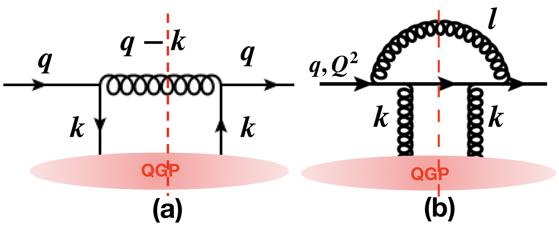
Figure 6: Forward scattering diagrams for future outlook. (a) Transverse broadening due to flavor changing process. (b) A typical single scattering and single emission diagram.

References

- Majumder and Van Leeuwen (2011) A. Majumder and M. Van Leeuwen, Prog. Part. Nucl. Phys. 66, 41 (2011), arXiv:1002.2206 [hep-ph] .
- Cao and Wang (2020) S. Cao and X.-N. Wang, (2020), arXiv:2002.04028 [hep-ph] .
- Burke et al. (2014) K. M. Burke et al. (JET Collaboration), Phys. Rev. C90, 014909 (2014), arXiv:1312.5003 [nucl-th] .
- Adler et al. (2007) S. S. Adler et al. (PHENIX), Phys. Rev. C76, 034904 (2007), arXiv:nucl-ex/0611007 .
- Adare et al. (2010) A. Adare et al. (PHENIX), Phys. Rev. Lett. 105, 142301 (2010), arXiv:1006.3740 [nucl-ex] .
- Adams et al. (2007) J. Adams et al. (Star), Phys. Rev. C75, 034901 (2007), nucl-ex/0607003 .
- Adler et al. (2003) C. Adler et al. (STAR), Phys. Rev. Lett. 90, 082302 (2003), nucl-ex/0210033 .
- Chatrchyan et al. (2014a) S. Chatrchyan et al. (CMS), Phys. Rev. Lett. 113, 132301 (2014a), [Erratum: Phys. Rev. Lett.115,no.2,029903(2015)], arXiv:1312.4198 [nucl-ex] .
- Acharya et al. (2018) S. Acharya et al. (ALICE), Phys. Lett. B776, 249 (2018), arXiv:1702.00804 [nucl-ex] .
- Cole (2011) B. A. Cole (ATLAS Collaboration), J.Phys. G38, 124021 (2011).
- Abelev et al. (2014) B. Abelev et al. (ALICE), JHEP 03, 013 (2014), arXiv:1311.0633 [nucl-ex] .
- Chatrchyan et al. (2014b) S. Chatrchyan et al. (CMS), Phys. Rev. C90, 024908 (2014b), arXiv:1406.0932 [nucl-ex] .
- CMS-PAS-HIN-11-004 (925220) CMS-PAS-HIN-11-004 925220, (2011).
- Aad et al. (2015) G. Aad et al. (ATLAS), Phys. Rev. Lett. 114, 072302 (2015), arXiv:1411.2357 [hep-ex] .
- Shuryak (1980) E. V. Shuryak, Phys. Rept. 61, 71 (1980).
- Shuryak (1978) E. V. Shuryak, Phys. Lett. B78, 150 (1978).
- Bazavov et al. (2019) A. Bazavov et al. (HotQCD), Phys. Lett. B 795, 15 (2019), arXiv:1812.08235 [hep-lat] .
- Borsanyi et al. (2020) S. Borsanyi, Z. Fodor, J. N. Guenther, R. Kara, S. D. Katz, P. Parotto, A. Pasztor, C. Ratti, and K. K. Szabo, Phys. Rev. Lett. 125, 052001 (2020), arXiv:2002.02821 [hep-lat] .
- Gyulassy and Wang (1994) M. Gyulassy and X.-N. Wang, Nucl. Phys. B420, 583 (1994), nucl-th/9306003 .
- Baier et al. (1995) R. Baier, Y. L. Dokshitzer, S. Peigne, and D. Schiff, Phys. Lett. B345, 277 (1995), arXiv:hep-ph/9411409 .
- Wang et al. (1995) X.-N. Wang, M. Gyulassy, and M. Plumer, Phys. Rev. D51, 3436 (1995), arXiv:hep-ph/9408344 .
- Baier et al. (1997a) R. Baier, Y. L. Dokshitzer, A. H. Mueller, S. Peigne, and D. Schiff, Nucl. Phys. B484, 265 (1997a), hep-ph/9608322 .
- Frenkel and Taylor (1990) J. Frenkel and J. C. Taylor, Nucl. Phys. B334, 199 (1990).
- Braaten and Pisarski (1990a) E. Braaten and R. D. Pisarski, Phys. Rev. Lett. 64, 1338 (1990a).
- Braaten and Pisarski (1990b) E. Braaten and R. D. Pisarski, Nucl.Phys. B337, 569 (1990b).
- Arnold et al. (2002) P. Arnold, G. D. Moore, and L. G. Yaffe, JHEP 06, 030 (2002), hep-ph/0204343 .
- Baier (2003) R. Baier, Nucl. Phys. A715, 209 (2003), arXiv:hep-ph/0209038 .
- Baier et al. (1997b) R. Baier, Y. L. Dokshitzer, A. H. Mueller, S. Peigne, and D. Schiff, Nucl. Phys. B483, 291 (1997b), hep-ph/9607355 .
- Song et al. (2011) H. Song, S. A. Bass, U. Heinz, T. Hirano, and C. Shen, Phys. Rev. Lett. 106, 192301 (2011), [Erratum: Phys. Rev. Lett.109,139904(2012)], arXiv:1011.2783 [nucl-th] .
- Shen et al. (2011) C. Shen, U. Heinz, P. Huovinen, and H. Song, Phys. Rev. C84, 044903 (2011), arXiv:1105.3226 [nucl-th] .
- Huovinen and Petreczky (2010) P. Huovinen and P. Petreczky, Nucl. Phys. A837, 26 (2010), arXiv:0912.2541 [hep-ph] .
- Majumder (2013) A. Majumder, Phys. Rev. C87, 034905 (2013).
- Politzer (1973) H. D. Politzer, Phys. Rev. Lett. 30, 1346 (1973).
- Gross and Wilczek (1973) D. J. Gross and F. Wilczek, Phys. Rev. Lett. 30, 1343 (1973).
- Ji (2013) X. Ji, Phys. Rev. Lett. 110, 262002 (2013), arXiv:1305.1539 [hep-ph] .
- Panero et al. (2014) M. Panero, K. Rummukainen, and A. Schäfer, Phys. Rev. Lett. 112, 162001 (2014), arXiv:1307.5850 [hep-ph] .
- Laine and Rothkopf (2014) M. Laine and A. Rothkopf, PoS LATTICE2013, 174 (2014), arXiv:1310.2413 [hep-ph] .
- Antonov and Pirner (2008) D. Antonov and H. J. Pirner, Eur. Phys. J. C 55, 439 (2008), arXiv:0710.1540 [hep-ph] .
- Note (1) The derivatives in the higher-twist terms include contributions from momenta up to the cutoff . With rare exceptions higher-dimensional operators suffer linearly divergent mixing with lower-dimensional operators in lattice regularization Gockeler et al. (1996), which persist after vacuum subtraction [Eq. (11\@@italiccorr)] due to temperature dependence.
- Note (2) The energy-momentum tensor’s temperature independent renormalization factor, which applies to the leading-twist term [Eq. (11\@@italiccorr)], has been obtained for Wilson’s plaquette action in pure gauge theory Giusti and Pepe (2014, 2015, 2017) using the shifted boundary condition approach Giusti and Meyer (2011a, b, 2013). This approach also carries over to QCD with sea quarks.
- Note (3) The bare and renormalized gluon and quark contributions to the energy-momentum tensor (EMT) are related by a mixing matrix. Details of this mixing are discussed in the Supplemental Material Sup . This precludes obtaining a continuum limit in QCD unless the quark contribution and the full mixing matrix are properly accounted for.
- Note (4) Operators with odd powers of the covariant derivative in Eq. (11\@@italiccorr) are odd under parity, and thus their expectation value vanishes on ensembles generated with an action that is invariant under parity. Operators mixing magnetic and electric field strengths that are included in Eq. (11\@@italiccorr) are related to the sextet representation of the energy-momentum tensor, and hence vanish on ensembles with standard boundary conditions, i.e. in the rest frame.
- (43) See Supplemental Material for details about parameter settings used in generating gauge ensembles, temperature dependence of the higher-twist operators, renormalization of operators in pure SU(3) and full QCD case, and radiative renormalization factors .
- MIL (2017) MILC collaboration code for lattice QCD calculations, public version on GitHub, https://github.com/milc-qcd/milc_qcd/ ; (2017).
- (45) SciDAC software modules for optimization: QDP-1.11.1, QIO-2.5.0, QLA-1.9.0, QMP-2.5.1, QOPQDP-0.21.1; https://www.usqcd.org/usqcd-software/ .
- Clark et al. (2005) M. Clark, A. Kennedy, and Z. Sroczynski, Nucl. Phys. B Proc. Suppl. 140, 835 (2005), arXiv:hep-lat/0409133 .
- Follana et al. (2007) E. Follana, Q. Mason, C. Davies, K. Hornbostel, G. P. Lepage, J. Shigemitsu, H. Trottier, and K. Wong, Physical Review D 75 (2007), 10.1103/physrevd.75.054502.
- Bazavov et al. (2014) A. Bazavov et al. (HotQCD), Phys. Rev. D 90, 094503 (2014), arXiv:1407.6387 [hep-lat] .
- Bazavov et al. (2018a) A. Bazavov, N. Brambilla, P. Petreczky, A. Vairo, and J. H. Weber (TUMQCD), Phys. Rev. D 98, 054511 (2018a), arXiv:1804.10600 [hep-lat] .
- Bazavov et al. (2016) A. Bazavov, N. Brambilla, H. T. Ding, P. Petreczky, H. P. Schadler, A. Vairo, and J. Weber, Phys. Rev. D 93, 114502 (2016), arXiv:1603.06637 [hep-lat] .
- Bazavov et al. (2018b) A. Bazavov, P. Petreczky, and J. Weber, Phys. Rev. D 97, 014510 (2018b), arXiv:1710.05024 [hep-lat] .
- Wilson (1974) K. G. Wilson, Phys. Rev. D10, 2445 (1974).
- Giusti and Pepe (2017) L. Giusti and M. Pepe, Phys. Lett. B 769, 385 (2017), arXiv:1612.00265 [hep-lat] .
- Giusti and Pepe (2015) L. Giusti and M. Pepe, Phys. Rev. D 91, 114504 (2015), arXiv:1503.07042 [hep-lat] .
- Capitani (2003) S. Capitani, Phys. Rept. 382, 113 (2003), arXiv:hep-lat/0211036 [hep-lat] .
- Soltz (2019) R. Soltz (Jetscape), PoS HardProbes2018, 048 (2019).
- He et al. (2015) Y. He, T. Luo, X.-N. Wang, and Y. Zhu, Phys. Rev. C91, 054908 (2015), [Erratum: Phys. Rev.C97,no.1,019902(2018)], arXiv:1503.03313 [nucl-th] .
- Qin and Majumder (2010) G.-Y. Qin and A. Majumder, Phys.Rev.Lett. 105, 262301 (2010), arXiv:0910.3016 [hep-ph] .
- Caron-Huot (2009) S. Caron-Huot, Phys. Rev. D 79, 065039 (2009), arXiv:0811.1603 [hep-ph] .
- Blaizot et al. (2013) J.-P. Blaizot, F. Dominguez, E. Iancu, and Y. Mehtar-Tani, JHEP 01, 143 (2013), arXiv:1209.4585 [hep-ph] .
- Blaizot and Mehtar-Tani (2014) J.-P. Blaizot and Y. Mehtar-Tani, Nucl. Phys. A 929, 202 (2014), arXiv:1403.2323 [hep-ph] .
- Liou et al. (2013) T. Liou, A. H. Mueller, and B. Wu, Nucl. Phys. A 916, 102 (2013), arXiv:1304.7677 [hep-ph] .
- Gockeler et al. (1996) M. Gockeler, R. Horsley, E.-M. Ilgenfritz, H. Perlt, P. E. L. Rakow, G. Schierholz, and A. Schiller, Phys. Rev. D 54, 5705 (1996), arXiv:hep-lat/9602029 .
- Giusti and Pepe (2014) L. Giusti and M. Pepe, Phys. Rev. Lett. 113, 031601 (2014), arXiv:1403.0360 [hep-lat] .
- Giusti and Meyer (2011a) L. Giusti and H. B. Meyer, Phys. Rev. Lett. 106, 131601 (2011a), arXiv:1011.2727 [hep-lat] .
- Giusti and Meyer (2011b) L. Giusti and H. B. Meyer, JHEP 11, 087 (2011b), arXiv:1110.3136 [hep-lat] .
- Giusti and Meyer (2013) L. Giusti and H. B. Meyer, JHEP 01, 140 (2013), arXiv:1211.6669 [hep-lat] .
- Hasenfratz and Hasenfratz (1980) A. Hasenfratz and P. Hasenfratz, , 241 (1980).
- Booth et al. (2001) S. Booth et al. (QCDSF-UKQCD), Phys. Lett. B 519, 229 (2001), arXiv:hep-lat/0103023 .
- Deur et al. (2016) A. Deur, S. J. Brodsky, and G. F. de Téramond, Progress in Particle and Nuclear Physics 90, 1 (2016).
- Philipsen (2013) O. Philipsen, Prog. Part. Nucl. Phys. 70, 55 (2013), arXiv:1207.5999 [hep-lat] .
- Note (5) The EMT’s off-diagonal components, which are in a nonet representation in the continuum, split into a triplet and a sextet in the discretized theory.
- Weber et al. (2019) J. H. Weber, A. Bazavov, and P. Petreczky, PoS Confinement2018, 166 (2019), arXiv:1811.12902 [hep-lat] .
- Laine and Schroder (2006) M. Laine and Y. Schroder, Phys. Rev. D 73, 085009 (2006), arXiv:hep-ph/0603048 .
- Haque et al. (2014) N. Haque, A. Bandyopadhyay, J. O. Andersen, M. G. Mustafa, M. Strickland, and N. Su, JHEP 05, 027 (2014), arXiv:1402.6907 [hep-ph] .
- Capitani and Rossi (1995) S. Capitani and G. Rossi, Nucl. Phys. B 433, 351 (1995), arXiv:hep-lat/9401014 .
- Dalla Brida et al. (2020) M. Dalla Brida, L. Giusti, and M. Pepe, JHEP 04, 043 (2020), arXiv:2002.06897 [hep-lat] .